Kernel Analog Forecasting:
Multiscale Test Problems

Abstract

Data-driven prediction is becoming increasingly widespread as the volume of data available grows and as algorithmic development matches this growth. The nature of the predictions made, and the manner in which they should be interpreted, depends crucially on the extent to which the variables chosen for prediction are Markovian, or approximately Markovian. Multiscale systems provide a framework in which this issue can be analyzed. In this work kernel analog forecasting methods are studied from the perspective of data generated by multiscale dynamical systems. The problems chosen exhibit a variety of different Markovian closures, using both averaging and homogenization; furthermore, settings where scale-separation is not present and the predicted variables are non-Markovian, are also considered. The studies provide guidance for the interpretation of data-driven prediction methods when used in practice.

37M10, 34E13, 58J65

1 Introduction

Data-driven prediction holds great promise in many areas of science and engineering. Growth in the volume of data available in numerous application areas has been matched by advances in computational methodologies which are designed to utilize this data for prediction. However fundamental questions arise in this field relating to the choice of variables on which to base prediction, and whether or not the system is Markovian in the chosen variables. Whilst delay embedding can be used to enhance the choice of variables in which Markovian structure is present, prediction is often undertaken using variables in which there is not a Markovian closure or in which this closure is only approximate. The objective of the paper is to use multiscale systems to provide a framework in which the fundamental issue of the role of Markovianity in data-driven prediction can be studied. We work within the setting of kernel analog forecasting (KAF), a methodology that has seen success in a number of application domains, and which is backed by a mature theory. Subsection 1.1 provides an overview of relevant literature in data-driven prediction for dynamical systems and the multiscale setting in which we work. We outline our contributions to the understanding of data-driven prediction within multiscale systems in Subsection 1.2.

1.1 Background And Literature Review

In 1969, Lorenz originally introduced the idea of analog forecasting for prediction of dynamical systems using historical data [30]. Given initial data, the method locates its closest analog among the historical points and reports the historical value of the corresponding observable, shifted by the desired lead time. By construction, analog forecasting avoids model error, but the resulting forecast is not continuous with respect to initial data. It is therefore non-physical and this fact, when combined with the paucity of data available at the time the method was proposed, limited the value of the methodology in practice. An exponential growth in data volume has precipitated the development of improved methodologies which build on Lorenz’s original idea, leading to algorithms which are backed by large data theories and which depend smoothly on initial condition. This has been achieved through the use of kernel based methods which result in data-driven prediction based on weighting all the historical data according to its similarity to the initial data; this leads to algorithms which enforce continuity of the forecast with respect to initial data [55] and, building on the theory of reproducing kernel Hilbert spaces [3], to algorithms which can be theoretically justified in the large data limit [16, 1].

KAF draws upon several fundamental ideas rooted in kernel methods for machine learning. First, the choice of kernel function is guided by the need for dimension reduction of big data and the specific learning task at hand. For clustering, similarity kernels [43] are used to construct graphs over the data, and clusters determined by its graph Laplacian eigenvectors [4]. This graph Laplacian construction is generalized in [10] to characterize diffusion operators on the manifold upon which the data lie via their eigenfunctions, known as diffusion maps, and further generalized in [7] to a class of variable-bandwidth kernels that control for variations in the density of the sampling distribution. Under different choices of kernel and normalization, the resulting eigenmaps can describe slow coordinates in dynamical systems [36], and can also be used as a basis to approximate evolution operators in stochastic differential equations (SDEs) [6]. Algorithmic development has been aided by advances in the theory for pointwise [45] and spectral [50, 47] convergence of these coordinates in the large data limit. Secondly, Markov operators constructed from kernels map into reproducing kernel Hilbert spaces (RKHSs) in which kernel evaluation corresponds to function evaluation, and allow evaluating these eigencoordinates on out-of-sample data [11] in a procedure known as Nyström extension. This has found use in semi-supervised classification using support vector machines [44] to extend labels to new data, spline interpolation [51], and forecasting [55].

In addition to exploiting ideas from kernel methods for machine learning, KAF may exploit additional structure from time-ordered data arising from dynamical systems. For example delay embedding is frequently used to identify Markovian structure. In diffusion forecasting [6], diffusion maps are time-shifted to approximate the action of a shift operator on observables in SDEs. Alternatively, time-shifted diffusion maps can be used to approximate the reduction coordinates of this shift operator directly [16], or, temporal structure can be directly embedded into specialized cone kernels for analog forecasting [55]. The latter takes the Nyström extension perspective of KAF, while in fact, KAF evaluates a conditional expectation of this shift operator, conditioned on the observations [1]. The aforementioned shift operator known as the Koopman operator acts by composing observables with the dynamical flow map, and is a linear operator on these function spaces. Hence, the data-driven approximation of the Koopman operator is an exciting area of research.

Bernhard Koopman introduced the linear operator that carries his name in the 1930s as part of his study of ergodic and Hamiltonian dynamics [27]. In data-driven identification of coherent structures spectral decompositions of the Koopman operator [34] and the related transfer operator [14] play a central role, driven by the fact that in such a basis, forecasting of nonlinear dynamics amounts to scalar multiplication by eigenvalues. Algorithms used in practice compute finite-dimensional regression onto pre-computed libraries consisting of functions of the time-lagged snapshots [42, 41, 26]. However, convergence guarantees are limited, requiring stringent assumptions on the libraries and spectrum [2]. In particular mixed spectra resulting from chaotic/mixing systems pose a challenge for numerical methods. Recent data-driven methods which leverage infinite-dimensional feature spaces provided by kernels [17], as well as kernel constructions in spectral space [28], are able to tackle the continuous part of the spectrum of the Koopman operator. For forecasting purposes, pointwise evaluation of the Koopman operator acting on observables is the natural setting, rather than spectral approximation, and is the perspective we take.

Multiscale analysis provides a setting in which to understand the role of rapidly varying (in space or time) system components on the slowly varying variables used for predictive models [53]. In this paper we will work in the framework of averaging and homogenization for partial differential equations (PDEs) and SDEs, as developed in [5]. Chapters 9, 10 and 11 of the book [38] contain a pedagogical exposition of the subject that is adapted to the chaotic deterministic ordinary differential equations setting that is the focus of this paper. However the rigorous extension of the theory of averaging and homogenization to ODEs, rather than SDEs, is non-trivial and less well-developed. Early work in this direction was contained in [37]. However it was not until the fundamental work of Melbourne and co-workers that a theoretical approach with verifiable conditions was developed [32, 33, 24, 23].

We will use the example developed in [33], which exploits the (proven) chaotic properties of the Lorenz 63 model [29, 48], to provide an example of a chaotic ordinary differential equation (ODE) which homogenizes to give an SDE. And we will use the multiscale Lorenz 96 model [31] to provide an example of an ODE to which the averaging principle may be applied to effect dimension reduction, as pioneered and exploited in [15]; we note, however, that the mixing properties required to prove the averaging principle for the Lorenz 96 model have not been established, even though numerical evidence strongly suggests that it applies in certain parameter regimes. The work of Jiang and Harlim [22] studies data-informed model-driven prediction in partially observed ODEs, using ideas from kernel based approximation; and in the paper [21] the idea is generalized to discrete time dynamical systems, and neural networks and LSTM modeling is used in place of kernel methods. In both the papers [22, 21] multiscale systems are used to test their methods in certain regimes.

Data-driven analog forecasting, kernel methods, and Koopman methodologies have each individually found widespread use in real-world forecasting and coherent pattern extraction applications. Analog forecasting, albeit without kernels, has been used to predict weather patterns [8, 13, 49], yet is known to have limitations predicting chaotic behavior. Khodkar et al. recently developed a Koopman-based framework using delay embedded observables to predict chaotic dynamics [25]. Nonlinear Laplacian spectral analysis, which applied kernel and delay embeddings akin to Koopman observables, successfully recovers coherent oscillatory phenomena such as the seasonal/diurnal cycles and the El Niño Southern oscillation [46] through kernel eigenfunctions [12]. Implemented with such kernels, KAF would naturally capture the fundamental oscillatory components of the predictand variable, and thus interpolate between an initial-value (“weather”) forecast at short times and a climatology forecast at asymptotic times when the mixing component of the predictand has decayed; e.g. [52]. Koopman operator approximation has also been widely adopted to study high-dimensional complex, even turbulent fluid flows [18], see [35] for a study of these applications.

In this paper we use KAF as developed in the papers [1, 16, 55]. Technical details on the implementation, including pseudocode and further relevant references, are collected in Appendix A.

1.2 Our Contribution

We use multiscale methodology to introduce four classes of ODE test problems which exhibit Markovian dynamics after elimination of fast variables; stochastic, chaotic, quasiperiodic and periodic behavior may be obtained in the slow variable, depending on the setting considered. Using these test problems, our four main contributions to the understanding of KAF are as follows:

1. We apply KAF techniques to data generated by each of these four classes of multiscale test problems, and use the behaviour of the averaged or homogenized slow system to interpret the resulting predictions. In particular, KAF methods converge, in the large data limit, to a conditional expectation defined via the Koopman operator of the multiscale systems; we use this as the basis for our interpretation. Moreover, we demonstrate the use of KAF to estimate the variance of the predictor itself. In each of the four cases the 2$\sigma$-interval captures the real trajectory, even when the KAF predictor does not track the trajectory itself. This can be viewed as a separate application of the KAF methodology which will be useful in cases when forecasting of high probability bounding sets suffices even when the trajectory itself is hard to predict. In all cases we also study problems in which the scale-separation is not present, but KAF prediction of mean and variance is attempted on the basis of data from only a subset of the variables.

2. The KAF method is based on data-driven approximation of the eigenvalue problem arising from a kernel integral operator. In the setting in which the multiscale ODE homogenizes to produce an SDE corresponding to a bistable gradient system with additive noise, a limiting analytical expression is available for the eigenfunctions; we demonstrate that these limiting eigenfunctions are well-approximated by the data-driven method. This comparison gives insight into the empirical methods used to tune free parameters within KAF.

3. In the setting in which the multiscale ODE averages to produce an ODE of lower dimension we use alternative data-driven ODE closures as a benchmark against which to compare the purely data-driven KAF methods. This gives insight into the relative merits of purely data-driven prediction, and prediction which combines model-based knowledge with data.

4. We use the insights from these carefully constructed numerical experiments to make recommendations about deployment, and parameter-tuning, of KAF methods to real data.

The paper is organized as follows. In Section 2, we outline the data-driven construction of the prediction function using KAF methodology. We explain the sense in which the construction converges to a conditional expectation defined via the Koopman operator associated to a measure-preserving dynamical system assumed to underlie the data. We also describe two kinds of canonical multiscale systems which give rise to homogenization and averaging effects, and which we use to provide interpretation of this conditional expectation. Section 3 introduces a test problem in the form of a double-well gradient flow driven by chaotic Lorenz 63 dynamics which homogenizes to give an SDE in the scale-separated regime; numerical results applied to prediction of the slow variable exhibit contributions 1 and 2. In section 4, we introduce the multiscale Lorenz 96 system which averages to give an ODE in the slow variables; three different parametric regimes give rise to periodic, quasiperiodic, and chaotic responses in the slow variable. The behaviour of KAF-based prediction in these three regimes is studied, to illustrate contribution 1; and a slow-variable closure model, built using Gaussian process regression, is compared with the KAF to illustrate contribution 3. In section 5 we overview the insights obtained by studying KAF methods through the lens of multiscale systems; and we then make concrete recommendations about interpreting the output of KAF techniques when applied to naturally occurring data, contribution 4.

2 Methodology

In subsection 2.1 we overview the two key ideas which interact to underpin the studies in this paper: KAF and multiscale methods, tailoring the exposition to the use of the latter as a tool to understand the former. We then give more details on KAF. The two primary components of the KAF methodology are: (i) viewing forecasting as evaluation of a conditional expectation of the Koopman operator applied to the desired observable; (ii) approximation of this conditional expectation in a data-driven fashion. Subsections 2.2 and 2.3 describe (i) and (ii) respectively, whilst subsection A.2 is devoted to a key practical component of the data-driven approximation, namely construction of the kernel, and subsection A.3 to the data-driven choice of integer $\ell$, the number of (approximate) eigenfunctions used in the data-driven forecast.

2.1 Overview Of Methodology

The problem setting for prediction is as follows. We assume that we are given $N$ time-ordered data samples

$$\{x_{n}\}_{n=0}^{N-1}\subset\mathcal{X},$$

where $x:\mathbb{R}\to\mathcal{X}$ is a continuous time process, $x_{n}=x(n\Delta t)$ and $\Delta t$ is the sampling rate. We assume that the continuous time process $x$ in $\mathcal{X}$ is derived from Markovian dynamics for a coupled pair $(x,y)$ evolving in the larger state space $\mathcal{X}\times\mathcal{Y}$. Assume that the desired prediction lead time $\tau$ is an integer multiple of the sampling interval, that is, $\tau=q\Delta t$. Included with the data are values of the associated prediction observable advanced by $\tau$ time units

$$\{f_{n+q}\}_{n=0}^{N-1}\subset\mathbb{R},$$

defined by the Markovian dynamics via an unknown map $F\colon\mathcal{X}\times\mathcal{Y}\to\mathbb{R}$; thus $f_{n}=F(x_{n},y_{n}).$ The goal of KAF is to predict $F(x(\tau),y(\tau))$ given only partial information, $x(0)=x$, and the $N$ data samples $x_{n}$. We view the data-driven predictor as a map $Z_{\tau}\colon\mathcal{X}\to\mathbb{R}$ which takes initial condition $x$ as input.

Given initial data $x$ and lead time $\tau$, the KAF predictor averages over the $\tau$-shifted observable values provided in the training data and weighted by a kernel $p:\mathcal{X}\times\mathcal{X}\rightarrow\mathbb{R}$ constructed from the data; the resulting algorithm has the following form:

(1) $$Z_{\tau}(x) =\frac{1}{N}\sum_{n=0}^{N-1}p(x,x_{n})f_{n+q},$$

$$p(x,x_{n}) =\sum_{j=0}^{\ell(\tau)-1}\frac{\psi_{j}(x)\phi_{j}(x_{n})}{\lambda_{j}^{1/2}}.$$

The weighting kernel $p(x,x_{n})$ determines how much weight to attach to a time-series initialized at point $x_{n}$, according to its proximity to $x$, the desired initial point. The features $\phi_{j}$ are computed from an eigenvalue problem associated with a data-driven approximation of a kernel integral operator, constructed from $x_{n}$; in the large data limit this provides an orthonormal basis for the entire space. The function $\psi_{j}$ is an out-of-sample Nyström extension of $\phi_{j}$, orthonormalized with respect to an underlying RKHS structure. The method may be seen as a smoothed version of Lorenz’s original proposal for data-driven prediction – analog forecasting [30]. Analog forecasting, by contrast, predicts the trajectory in the training data obtained by finding the training data point nearest to the given initial condition in some metric $d:\mathcal{X}\times\mathcal{X}\rightarrow\mathbb{R}$

(2) $$Z_{\tau}(x)=f_{n^{\star}+q},\quad\quad n^{\star}=\operatorname*{arg\,min}_{n=0,\dots,N-1}d(x,x_{n}).$$

It can be seen that Lorenz’ method will result in predictions discontinuous with respect to initial data, especially for systems that exhibit sensitive dependence on initial conditions. In particular, KAF addresses the issue of continuity of the prediction with respect to the initial condition, and it does so in a framework which is provably statistically consistent in the large data limit [1, 16, 55]. Further details of the methodology are given in the next two subsections, and the attendant information in Appendix A.

An important challenge addressed by this methodology is that, since the $y$ component of the system is not observed, the sequences $\{x_{n}\}$ and $\{f_{n+q}\}$ are non-Markovian. As a consequence the standard idea of constructing a Markov chain from the data is not natural. The kernel analog forecasting method evaluates a conditional expectation of the forecast conditioned, using the observed data $\{x_{n}\}$, explicitly incorporating information loss resulting from unobserved $y$; it is hence a natural approach to the problem at hand. Multiscale systems provide a natural setting for the study of KAF methods, and in particular the issue of prediction of non-Markovian or approximately Markovian systems. In this paper we will consider the variable $x$ as the slow component of a Markovian system for pair $(x,y)$ in which $y$ evolves as a fast variable. We consider averaging and homogenization settings in which the dynamics for $x$ is approximately Markovian, and the conditional expectation arising in the KAF method may be understood explicitly. This will enable us to obtain a deeper understanding of how KAF works, and help users of the methodology interpret it. We now outline the averaging and homogenization settings that we will use. Details of the theory underlying them may be found in [38].

We will study multiscale systems which exhibit averaging, in the form

(A) $$\begin{cases}&\dot{x}=v_{0}(x)+By,\\ &\dot{y}=\frac{1}{\varepsilon}g(x,y),\end{cases}.$$

where $B\colon\mathcal{Y}\to\mathcal{X}$ is linear. The average of $By$ under the invariant measure of the $y$ dynamics, with $x$ frozen, provides a closed approximate ODE dynamics for $x$, when $\varepsilon$ is small. If we denote the $x-$parameterized invariant measure for the $y$ dynamics with $x$ frozen by $\nu^{x}(dy)$ then for $\varepsilon\ll 1$ we obtain $x\approx X$ where

(A0) $$\dot{X} =v_{0}(X)+v(X),$$

$$v(\zeta) =\int_{\mathcal{Y}}By\,\nu^{\zeta}(dy).$$

To guarantee uniqueness of solutions in (A0), it suffices that the conditional measure has enough continuity, as a function of $x$, so that $v(\zeta)$ is Lipschitz.

When the variable $By$ averages to zero a different scaling is required to elicit the effect of the fast variable on the slow one. To this end we also consider multiscale systems which exhibit homogenization, in the form

(H) $$\begin{cases}&\dot{x}=v_{0}(x)+\frac{1}{\varepsilon}By\\ &\dot{y}=\frac{1}{\varepsilon^{2}}g(y)\end{cases}$$

Here we assume that

$$\int_{\mathcal{Y}}By\,\nu(dy)=0$$

where $\nu$ is the invariant measure of the $y$ dynamics. The approximate dynamics for $x$, when $\varepsilon$ is small, is then governed by an SDE in this setting; the work of Melbourne and co-workers provides the sharpest results in this context [32, 33, 24, 23]. If this is the case then, invoking the homogenization principle, $x\approx X$ where $X$ is governed by an SDE of the form

(H0) $$\dot{X}=v_{0}(X)+\sqrt{2\sigma}\dot{W},$$

where $W$ denotes the Wiener process, and $\sigma$ is a uniquely determined positive constant that can be computed numerically from the mixing properties of the $y$ process.

2.2 Koopman Formulation Of Prediction

Koopman

Data-driven

Figure 1: Comparison of exact Koopman picture and data-driven approximation. The approximate mapping $Z_{\tau}(\cdot)$ is constructed from the data streams $\{H\Phi^{t}(x_{0},y_{0})\}_{0\leqslant t\leqslant T}$ and $\{F(\Phi^{t}(x_{0},y_{0}))\}_{0\leqslant t\leqslant T}.$

We let $\Omega=\mathcal{X}\times\mathcal{Y}$ and assume that $\Phi^{t}\colon\Omega\to\Omega$ is an ergodic dynamical system with invariant probability measure $\mu$; we assume $t\in\mathbb{R}^{+}$ but the extension to discrete time is straightforward. Define the continuous observation map ${\color[rgb]{0,0,0}\Pi}\colon\Omega\to\mathcal{X}$ and the prediction observable $F\colon\Omega\to\mathbb{R}$; we assume that $F$ is square-integrable with respect to the invariant measure:

$$F\in L^{2}_{\mu}(\Omega;\mathbb{R})\coloneqq\left\{F\colon\Omega\to\mathbb{R}\;\middle|\;\int_{\Omega}|F(\omega)|^{2}\mu(d\omega)<\infty\right\}.$$

We define the Koopman operator $U^{t}\colon L^{2}_{\mu}(\Omega;\mathbb{R})\to L^{2}_{\mu}(\Omega;\mathbb{R})$ by $U^{t}g=g\circ\Phi^{t}$. We seek, in a sense to be made precise, the function $Z_{\tau}\colon\mathcal{X}\to\mathbb{R}$ such that $Z_{\tau}\circ{\color[rgb]{0,0,0}\Pi}$ is the best approximation to a perfect prediction of $F\circ\Phi^{\tau}$. We formalize this by introducing the Hilbert subspace $V\subseteq L^{2}_{\mu}(\Omega;\mathbb{R})$ given by

$$V\coloneqq\left\{g\in L^{2}_{\mu}(\Omega;\mathbb{R})\;\middle|\;g=g^{\prime}\circ{\color[rgb]{0,0,0}\Pi},\;g^{\prime}\colon\mathcal{X}\to\mathbb{R}\right\}.$$

This Hilbert space captures the notion of making predictions based only on information in $\mathcal{X}$. Note that the perfect forecast would satisfy $Z_{\tau}\circ{\color[rgb]{0,0,0}\Pi}=U^{\tau}F$, but that such a forecast will not be possible in general because $\mathcal{X}$ is a proper subset of $\Omega$, and information needed for perfect prediction of $F$ will be missing. Among all elements of $V$, the minimal prediction error in $L^{2}_{\mu}(\Omega;\mathbb{R})$ is attained by the conditional expectation

(3) $$\operatorname{\mathbb{E}}(U^{\tau}F\mid{\color[rgb]{0,0,0}\Pi})=\operatorname*{arg\,min}_{g^{\prime}\in V}\lVert g^{\prime}-U^{\tau}F\rVert_{L^{2}_{\mu}}=\operatorname*{proj}_{V}U^{\tau}F.$$

This formulation of prediction encapsulates the inherent loss of information incurred through observing only a set of functionals of an ergodic dynamical system, and the effect of this loss of information on prediction. In subsequent sections of this paper we will assume that $F=F^{\prime}\circ{\color[rgb]{0,0,0}\Pi}$ for some $F^{\prime}:\mathcal{X}\to\mathbb{R}$ because it is often natural to try to predict only functionals of the slow variables. Note, however, that the methodology is not restricted to such $F$ and in this subsection, the next subsection and in Appendix A we describe the more general setting for completeness.

2.3 Data-Driven Approximation

The formulation in the preceding subsection encapsulates the inherent loss of predictive power incurred through observing only a set of functionals of an ergodic dynamical system. This is formalized by seeking the best approximation of the Koopman evolution from within a Hilbert subspace capturing the notion of depending only on specified functionals on the state space of the dynamical system. We now demonstrate how data may be used to further approximate this best approximation, and to do so in a manner which is refineable as more data is acquired. The approach is summarized in Figure 1.

For observation time $\Delta t>0$ we define

$$\omega_{n} =\Phi^{t_{n}}(\omega_{0}),\quad t_{n}=n\Delta t,$$

$$x_{n} ={\color[rgb]{0,0,0}\Pi}(\omega_{n}),\quad f_{n}=F(\omega_{n}).$$

We assume that we are given time-ordered pairs

(4) $$\{(x_{0},f_{q}),(x_{1},f_{1+q}),\ldots,(x_{N-1},f_{N-1+q})\},$$

and the objective is to construct, from this data, a function $Z_{\tau}\colon\mathcal{X}\to\mathbb{R}$ which predicts $F$ at lead time $\tau$ so that $Z_{\tau}\circ{\color[rgb]{0,0,0}\Pi}\approx g^{\star}$ where $g^{\star}$ solves the minimization problem in (3). Furthermore we wish to carry this out in a manner which ensures that, in an appropriate topology, $Z_{\tau}\circ{\color[rgb]{0,0,0}\Pi}\to g^{\star}$ as $N\to\infty$.

To this end we introduce a hypothesis space $\mathcal{H}_{\ell,N}$, of dimension $\ell$ and depending on the $N-$dependent data set (4), and seek to solve the minimization problem

(5) $$Z_{\tau}=\operatorname*{arg\,min}_{g\in\mathcal{H}_{\ell,N}}\lVert g\circ{\color[rgb]{0,0,0}\Pi}-U^{\tau}F\rVert_{L^{2}_{\mu}}.$$

The choice of the hypothesis space is constrained by the need to be able to solve the minimization problem (5) explicitly, using only the data (4), and by the requirement that $Z_{\tau}\circ{\color[rgb]{0,0,0}\Pi}$ recovers $g^{\star}$ in the large data limit $N\to\infty$. Moreover, in order to be practically useful forecast functions, elements of $\mathcal{H}_{\ell,N}$ should allow pointwise evaluation at any $x\in\mathcal{X}$, which is not defined in arbitrary subspaces of $L^{2}_{\mu}(\Omega;\mathbb{R})$.

With these considerations in mind, we introduce a kernel function $k\colon\mathcal{X}\times\mathcal{X}\to\mathbb{R}$ and RKHS $\mathcal{K}$ with the properties

$$f(x)=\langle k_{x},f\rangle_{\mathcal{K}},\quad k_{x}=k(x,\cdot),\quad\langle k_{x},k_{x^{\prime}}\rangle_{\mathcal{K}}=k(x,x^{\prime}).$$

We then define $\mathcal{H}_{\ell,N}$ as an $\ell$-dimensional subspace of $\mathcal{K}$, to be described below. We also note that the kernel $k$ is constructed from a data-stream of length $N$, but we suppress the explicit dependence of $k$ on $N$ in the notation. In Appendix A we discuss our data-driven construction of $k$, and choice of $\ell$. For now we proceed on the assumption that we have a kernel, and hence a RKHS, as well as a method for choosing $\ell.$

Let ${\mu}_{\scriptscriptstyle{N}}=\frac{1}{N}\sum_{n=0}^{N-1}\delta_{\omega_{n}}$ be the sampling measure underlying the training data (4) and define

$$L^{2}_{\mu_{N}}(\Omega;\mathbb{R})\coloneqq\left\{F\colon\Omega\to\mathbb{R}\;\middle|\;\int_{\Omega}|F(\omega)|^{2}{\mu}_{\scriptscriptstyle{N}}(d\omega)=\frac{1}{N}\sum|F(\omega_{n})|^{2}<\infty\right\}.$$

Associated with ${\mu}_{\scriptscriptstyle{N}}$ is an integral operator $G\colon L^{2}_{\mu_{N}}(\Omega;\mathbb{R})\to L^{2}_{\mu_{N}}(\Omega;\mathbb{R})$ which we identify with a symmetric, positive-semidefinite, $N\times N$ kernel matrix $G\in\mathbb{R}^{N\times N}$ with entries

(6) $$G_{mn}=k(x_{m},x_{n}),\quad x_{n}={\color[rgb]{0,0,0}\Pi}(\omega_{n}),\quad 0\leq m,n\leq N-1.$$

The eigenvectors of this matrix lead to an orthonormal basis $\{\phi_{j}\}_{j=0}^{N-1}$ of $\mathbb{R}^{N}$ such that

$$G\phi_{j}=\lambda_{j}\phi_{j},\quad\lambda_{0}\geq\lambda_{1}\geq\cdots\geq\lambda_{N-1},\quad\lVert\phi_{j}\rVert_{2}=\sqrt{N}.$$

We may also identify each element $\phi_{j}\in\mathbb{R}^{N}$ with element $\phi_{j}\circ{\color[rgb]{0,0,0}\Pi}\in L^{2}_{\mu_{N}}(\Omega;\mathbb{R})$ via the definition $\phi_{j}(x_{n})$ as the $n^{th}$ entry of the vector $\phi_{j}\in\mathbb{R}^{N}$. Using the same symbols for elements of $\mathbb{R}^{N}$ and $L^{2}_{\mu_{N}}(\Omega;\mathbb{R})$, as well as for linear transformations on those spaces, is a useful economy of notation. Then the following functions $\psi_{j}\colon\mathcal{X}\to\mathbb{R}$ form an orthonormal set in $\mathcal{K}$:

(7) $$\psi_{j}=\frac{1}{N\lambda_{j}^{1/2}}\sum_{n=0}^{N-1}k(\cdot,x_{n})\phi_{j}(x_{n}),\quad\lambda_{j}>0.$$

This is a form of Nyström extension [11].

As hypothesis space we take

(8) $$\mathcal{H}_{\ell,N}=\operatorname{span}\{\psi_{0},\cdots,\psi_{\ell-1}\}\subseteq\mathcal{K}$$

noting that the basis functions themselves depend on the data set, and hence on $N$. We may now solve the optimization problem (5) and an explicit computation yields, for $\tau=qT$,

(9) $$Z_{\tau}(x)=\sum_{j=0}^{\ell-1}\frac{c_{j}(\tau)}{\lambda_{j}^{1/2}}\psi_{j}(x),\quad c_{j}(\tau)=\langle\phi_{j}\circ{\color[rgb]{0,0,0}\Pi},U^{\tau}F\rangle_{L^{2}({\mu}_{\scriptscriptstyle{N}})}=\frac{1}{N}\sum_{n=0}^{N-1}\phi_{j}(x_{n})f_{n+q}.$$

Note that this construction of the predictor $Z_{\tau}$ is entirely data-driven: the basis functions $\psi_{j}$ and the eigenvalues $\lambda_{j}$ are found from the eigenvalues and eigenvectors of the data-defined kernel matrix; and the coefficients $c_{j}$ are computed as sums over the data set. Furthermore, Theorem 14 in [1] proves that $Z_{\tau}\circ X$ converges to $g^{\star}$, the solution of the minimization problem (3), as $N\to\infty$, followed by $\ell\to\infty$, in an $L^{2}$ sense with respect to the invariant measure $\mu$ on $\Omega.$

More generally, any function of the observable can be predicted in this data-driven manner, which provides a convenient framework for uncertainty quantification. The conditional variance between forecast and ground truth can also be computed in the hypothesis space as in (9) using the coefficients

(10) $$\hat{c}_{j}(\tau)=\langle\phi_{j}\circ{\color[rgb]{0,0,0}\Pi},(U^{\tau}F-Z_{\tau})^{2}\rangle_{L^{2}({\mu}_{\scriptscriptstyle{N}})}=\frac{1}{N}\sum_{n=0}^{N-1}\phi_{j}(x_{n})(f_{n+q}-Z_{\tau}(x_{n}))^{2}.$$

For detail on the data-driven kernel construction, the data-driven choice of $\ell$ and the conditional variance estimator see subsections A.2, A.3 and A.4 respectively.

3 Homogenization: Lorenz 63 Driven System

This section is devoted to the setting in which a chaotic ODE of form (H) is approximated by an SDE of form (H0). The goal is to make predictions of the $x$ variable, using data concerning only the $x$ variable from (H); the role of (H0) is simply to help us interpret those predictions. This setting presents unique challenges for forecasting as one cannot expect the outcome of any method to predict a sample path of a stochastic process without knowledge of the driving noise. This fact has direct bearing on prediction in (H) using $x$-data alone, since (H0) demonstrates that the time series of the $x-$data is approximately that of an SDE; without knowledge of the noise, which is governed by the unobserved $y$ variable, prediction of the trajectory of $x$ is not possible. In subsection 3.2 we examine instead the long-term statistics predicted by KAF from data generated by (H) — the conditional expectation and variance of the stochastic process — and compare them with estimates computed from (H0) using Monte-Carlo simulation of the SDE. This illustrates our main contribution 1 from the list in subsection 1.2. Then, in subsection 3.3, exploiting the fact that the limiting process is one-dimensional, we find explicit expressions for the kernel eigenfunctions in the limit problem (H0) and compare these with the eigenfunctions obtained from data-driven techniques applied to (H), our main contribution 2 from subsection 1.2. Subsection 3.4 is concerned with non-Markovian prediction, in which there is no scale-separation between observed and unobserved variables. We start, however, in subsection 3.1, introducing the concrete model around which our experiments are organized.

3.1 The Model

The first test problem arises from driving a double-well gradient flow with a chaotic signal obtained from the Lorenz 63 model [19]:

(11) $$\dot{x} =x-x^{3}+\frac{4}{90\varepsilon}y_{2},$$

$$\dot{y}_{1} =\frac{10}{\varepsilon^{2}}(y_{2}-y_{1}),$$

$$\dot{y}_{2} =\frac{1}{\varepsilon^{2}}(28y_{1}-y_{2}-y_{1}y_{3}),$$

$$\dot{y}_{3} =\frac{1}{\varepsilon^{2}}\left(y_{1}y_{2}-\frac{8}{3}y_{3}\right).$$

This is of form (H). In [33] it is proved that as $\varepsilon\to 0$ this system converges weakly in $C([0,T];\mathbb{R})$, when projected onto the $x$ variable alone, to solution of the SDE

(12) $$\dot{X} =-\Xi^{\prime}(X)+\sqrt{2\sigma}\dot{W},$$

$$\Xi(X) =\frac{1}{4}(X-X^{2})^{2}.$$

Thus, this white-noise driven gradient system is of form (H0). The value of the constant $\sigma$ is identified in [19]. For the current work the key point to appreciate is that for small $\varepsilon$ the variable $x$ in (11) exhibits (approximately) Markovian behaviour, but this behaviour is stochastic. The SDE is ergodic and has invariant probability density function

(13) $$\rho_{\infty}(x)\propto\exp\left(-\frac{1}{\sigma}\Xi(x)\right),$$

with respect to Lebesgue measure.

3.2 Conditional Expectation and Variance

We aim to predict the $x$ variable from historical data of a long trajectory of $x$ alone. Thus the observation and observable maps are ${\color[rgb]{0,0,0}\Pi}(\omega)=x,F(\omega)=x.$ We will also estimate second moments, enabling us to compute conditional variance, for which $F(\omega)=x^{2}.$ Observation data is generated by using an implicit time-stepping scheme with time-step $0.01$ in the slow variable and built-in Matlab solvers to integrate the fast variables with $\varepsilon=0.001$. Source data for the slow variable $x$ is gathered for $N=40000$ points sampled at the macroscopic time interval $\Delta t=0.05$. Then $\hat{N}=7500$ out-of-sample points from a new trajectory $\{\hat{x}_{n}\}$ are gathered at the same resolution, which provide the ground truth for assessing forecast error. The natural error metric is the root mean squared error (RMSE ), the $L^{2}$ norm of $Z_{\tau}-U^{\tau}F.$ To account for differences in scale, we normalize the RMSE by the standard deviation of the trajectory.

$${\sf{{RMSE}}\,}(\tau)=\bigg{(}\frac{1}{\hat{N}-q}\sum_{n=0}^{\hat{N}-q-1}|Z_{\tau}(\hat{x}_{n})-\hat{x}_{n+q}|^{2}\bigg{)}^{1/2}\bigg{(}\frac{1}{\hat{N}-q}\sum_{n=0}^{\hat{N}-q-1}|\hat{x}_{n+q}-\bar{x}|^{2}\bigg{)}^{-1/2}.$$

\begin{overpic}[width=260.17464pt]{forecastL6340k_idxX_1_OSE_l10} \put(45.0,-1.0){$\tau$} \put(100.0,30.0){\fcolorbox{black}{white}{\parbox{1.9cm}{\scriptsize{\color{gray} \bf--} Trajectory \\ {\color{black} \bf--} SDE mean \\ {\color{red} \bf--} SDE 2$\sigma$ \\ {\color{blue} \bf--} Prediction\\ {\color{pink}$\blacksquare$} Predicted 2$\sigma$ }}} \end{overpic}

Figure 2: Long-term forecast convergence. Grey: the trajectory of the SDE started from $x=-1.10$; blue the KAF predictor $Z_{\tau}(-1.10)$ with pink shades giving two standard deviation confidence bands computed from the conditional variance; black the Monte Carlo approximation of the conditional mean using the SDE; red the Monte Carlo approximation of the conditional variances using the SDE. KAF computations of mean and variance agree with the true conditional expectation and mean computed from $10000$ Monte Carlo realizations of the SDE.

\begin{overpic}[width=260.17464pt]{rmse_l63} \put(45.0,-1.0){$\tau$} \end{overpic}

Figure 3: Long-term RMSE  for the forecast in Figure 2 saturates at $\tau=50$, as the forecast converges to the long-term mean at $X=0$.

\begin{overpic}[width=260.17464pt]{forecastL63uq_x0_1_10.pdf} \put(100.0,33.0){\fcolorbox{black}{white}{\parbox{1.9cm}{\scriptsize{\color{gray} \bf--} Trajectory \\ {\color{blue} \bf--} Prediction\\ {\color{pink}$\blacksquare$} Predicted 2$\sigma$ }}} \end{overpic}

\begin{overpic}[width=260.17464pt]{forecastL63uq_x0_0_02.pdf} \put(50.0,0.0){$\tau$} \end{overpic}

Figure 4: Comparison of uncertainty for different initial data. Blue is predictor (conditional mean), grey is trajectory and pink gives two standard deviations bounds computed from the conditional variance. The forecast uncertainty when initialized at $x=0$ (right) displays more rapid growth in uncertainty over short lead times than that when $x=-1.10$ (left). This sensitivity to initial conditions is a desirable feature of KAF, in light of the fact that both plots share the same training set.

Figure 2 depicts the behavior of the KAF forecast $Z_{\tau}(x)$ as a function of lead time $\tau$, for fixed $x$. This forecast exhibits two interesting properties which can be understood through the small-$\varepsilon$ homogenization limit. The first relates to the fact that the trajectory itself is not well-predicted; the second explains what is well-predicted.

Firstly, the predictor tracks the conditional mean initialized at $x=-1.10$, and not the trajectory itself. This is predicted by the theory, since what is predicted is the long-term conditional expectation $\operatorname{\mathbb{E}}[U^{\tau}F|{\color[rgb]{0,0,0}\Pi}]$. Indeed this latter quantity necessarily converges for large $\tau$ to a constant, under mixing assumptions on the $(x,y)$ system, whilst individual trajectories in $x$ exhibit stochastic dynamics, approximately that of $X$. This explains the growth in RMSE seen in Figure 3. Secondly, exploiting the fact that we expect the system (11) to behave like (12), when projected onto the $x$ co-ordinate, we can provide an objective evaluation of the KAF forecasts by running Monte-Carlo simulations of the SDE for $X$; to do this we compute the sample mean and variance over $10000$ sample paths initialized at the same initial point $x=-1.10$. Figure 2 compares the KAF forecast mean and variance with that predicted by Monte-Carlo mean and variance for the SDE, and they are seen to agree very well over the entire window of computation.

Finally in Figure 4 we use the possibility of varying the initial condition in the KAF to demonstrate that the variability encapsulated in the conditional variance is able to pick-up different sensitivities, depending upon initial condition. The panel on the left shows a trajectory initialized at $x=-1.10$ and the panel on the left shows a trajectory initialized at $x=0.$ As can be expected from the limiting SDE, the uncertainty when initialized at $x=0$ is greater and this is manifest in the conditional variance.

Examination of the KAF technique in this homogenization setting thus clearly reveals the inability of the method to predict trajectories, but shows that it can accurately approximate statistics of trajectories, averaged over the unobserved component of the system. Furthermore, analysis of the SDE provides a means of characterizing the geometry of the underlying hypothesis space, as seen in the next subsection.

3.3 Insights Into The Hypothesis Space

By studying the large data and small kernel bandwidth limit of the matrix $G$ defined in (6) we get insights into the structure of the hypothesis space (8). The theory in [16], building on the papers [10, 7], demonstrates that, for the choice of kernel described in Appendix A, the vectors of $G$ are approximated in the large data and small bandwidth limit by eigenfunctions of the Laplace-Beltrami operator $\Delta_{h}$ on $M$, associated to a metric $h$. For the diffusion process (12) in dimension $m=1$ the manifold $M$ is simply $\mathbb{R}$ and the metric $h$ is given by $h=\rho^{-2}$, with invariant density $\rho$ given by (12). The fact that the density $\rho$ is approximately available to us through the time series $x$ generated by (11) is demonstrated in the left panel of Figure 5, where we compare the histogram generated by the data with $\rho$ given by (13). The conclusion of these various approximations is that we expect the eigenvectors of $G$, based on data $x$ from (11), to be well-approximated by eigenfunctions of $\Delta_{h}$ on $\mathbb{R}$, with $h=\rho^{-2}.$ We now demonstrate that this is indeed the case.

The action of the Laplace-Beltrami operator on $f\in C^{\infty}(M)$ is given by

$$\Delta_{h}f=-{\operatorname{div}}_{\mu}{\operatorname*{grad}}_{h}f=-{\operatorname{div}}_{\mu}\left(\frac{1}{\rho}\frac{df}{dX}\right)=-\frac{1}{\rho}\frac{d}{dX}\left(\frac{1}{\rho}\frac{df}{dX}\right),$$

where $\operatorname{div}_{\mu}$ and $\operatorname*{grad}_{h}$ are the divergence and gradient operators associated with $\mu$ and $h$, respectively. Using the above, we solve the eigenvalue problem $-\Delta_{h}\varphi=\lambda^{2}\varphi$ directly. We make the substitution $dY=\rho dX$, mapping $X\in\mathbb{R}$ into $Y\in[0,1]$; we note that $Y$ has interpretation as the cumulative distribution function coordinate of $\rho$. In terms of $Y$ we have

$$\Delta_{h}f=-\frac{1}{\rho}\frac{d}{dX}\left(\frac{1}{\rho}\frac{df}{dX}\right)=-\frac{d^{2}f}{dY^{2}}.$$

Noting that the natural boundary conditions for the Laplace-Beltrami operator are of no-flux type, it follows that, when viewed as functions of $Y$, the eigenfunctions of $\Delta_{h}$ satisfy a boundary value problem of the form

$$-\varphi^{\prime\prime}(Y)=\lambda^{2}\varphi(Y),$$

$$\varphi^{\prime}(0)=\varphi^{\prime}(1)=0.$$

The solutions are the well-known harmonics $\cos(k\pi Y),$ and corresponding eigenvalues $\lambda_{k}=k\pi,k\in\mathbb{N}$. Changing back to variable $x$ we obtain

(14) $$\varphi_{k}(X)=\cos\left(k\pi\int_{-\infty}^{X}\rho(z)dz\right).$$

\begin{overpic}[width=134.42113pt]{{hist_sigma_0.1091}.pdf} \put(40.0,80.0){\scriptsize$\rho_{\infty}(x)$} \end{overpic}

\begin{overpic}[width=138.76157pt]{phi_l7_color} \put(40.0,80.0){\scriptsize$\psi_{j}(x)$} \end{overpic}

\begin{overpic}[width=138.76157pt]{phi_true_l7_gray} \put(40.0,80.0){\scriptsize$\varphi_{j}(X)$} \end{overpic}

Figure 5: Comparison of invariant densities and eigenfunctions. Left: invariant density (13) and histogram of $x$ from (11). Middle and right: six empirically computed eigenfunctions using $x$ from (11), and using theory associated with (12), respectively.

We now verify that, for large data sets and small bandwidth, the eigenfunctions of $G$ are indeed close to those associated with the Laplace-Beltrami operator $\Delta_{h}.$ This is demonstrated in the middle and right panels of Figure 5. The middle panel shows the first six eigenfunctions of $G$, computed from data derived from the $x$ variable in (11); the right panel shows the eigenfunctions of $\Delta_{h}$ for diffusion process (12) in variable $X$ which governs the limiting behaviour of $x$ in the scale-separated case. The agreement is excellent, demonstrating that the heuristics underlying parameter choices within the kernel based methodology (see Appendix A) work well in this setting.

\begin{overpic}[width=260.17464pt]{forecast40k_1_l10.pdf} \put(40.0,37.0){\footnotesize${\color[rgb]{0,0,0}\Pi}(\omega)=x$} \put(100.0,33.0){\fcolorbox{black}{white}{\parbox{1.9cm}{\scriptsize{\color{gray} \bf--} Trajectory \\ {\color{blue} \bf--} Prediction\\ {\color{pink}$\blacksquare$} Predicted 2$\sigma$ }}} \end{overpic}

\begin{overpic}[width=260.17464pt]{forecast40k_13_eps1.pdf} \put(50.0,-2.0){$\tau$} \put(32.0,35.0){\footnotesize${\color[rgb]{0,0,0}\Pi}(\omega)=[x,4y_{2}/90]^{T}$} \end{overpic}

Figure 6: Prediction in non-Markovian regime, $\varepsilon=1$, requires observations augmented by the forcing term to achieve short-term predictability.

3.4 Non-Markovian Regime

In the preceding subsections we studied predictors for $x$, based only on time-series data in the $x$ coordinate, for the equation (11). We studied the scale-separated regime where $\varepsilon\ll 1$ and $x$ is approximately Markovian – it is approximately governed by an SDE. Here we study the behavior of identical predictors when $\varepsilon=1$; the system  (11) then no longer exhibits homogenization and $x$ is no longer Markovian in view of the lack of scale-separation. As a result, the prediction of $x$, shown in the top of Figure 6, is poor even at very short times, and the two standard deviation confidence bands reflect this rapid initial error growth, and then remain large throughout the time window. $Z_{\tau}$ converges rapidly to the conditional mean. To render the problem Markovian we may include more data, and in particular the forcing term. To this end we take ${\color[rgb]{0,0,0}\Pi}(\omega)=[x,4y_{2}/90]^{T}$; see the bottom of Figure 6. The prediction of $x$ with these augmented observations yields very accurate predictions over a lead time of $\tau=3$, considerably larger than in the preceding case where ${\color[rgb]{0,0,0}\Pi}(\omega)=x$. After $\tau=3$, however, pathwise predictability again fails, due to the sensitive dependence of solutions with respect to the forcing function. Once again $Z_{\tau}$ converges to the conditional mean. However the uncertainty quantification provided by two standard deviation error bars consistently captures the true trajectory, even in this non-Markovian regime.

This non scale-separated pair of examples illustrates that prediction of non-Markovian variables is inherently harder than Markovian variables, but that sensitive dependence of trajectories with respect to perturbations also limits predictability, even in the Markovian setting. This second point will be prominent, too, in the next section.

4 Averaging: Lorenz 96 Multiscale System

This section is devoted to the setting in which a chaotic ODE of form (A) is approximated by an ODE of form (A0). The goal is to make predictions of the $x$ variable using data concerning the $x$ variable alone from (A). The role of (A0) is primarily to help us interpret those predictions; however it also serves to motivate a different prediction methodology, which mixes model-based and data-driven methodologies, against which we will compare KAF.

The averaging setting presents interesting opportunities to understand forecasting. In particular, by tuning a parameter in (A), which is also present in (A0), we are able to create settings in which the variable to be predicted is, in turn, approximately periodic, quasi-periodic and chaotic. These different settings give rise to different types of forecasts and we demonstrate this. In subsection 4.2 we examine the long-term statistics predicted by KAF from data generated by (A) – the conditional expectation and variance of one component of the slow variable – and compare them with estimates computed from (A0) using Monte-Carlo simulation. This illustrates our main contribution 1 from the list in subsection 1.2. Then, in subsection 4.3, we compare the purely data-driven method of prediction with a hybrid data-model predictor. This hybrid is computed by using Gaussian process (GP) regression to compute an approximate closure $v_{\scriptscriptstyle{GP}}(x)\approx v(x)$, in the notation of (A0); for more details on such approximate closures in the context of the specific model we study in the following four subsections see [15] and references therein. The work in subsection 4.3 illustrates our main contribution 3 from subsection 1.2. Subsection 4.4 is concerned with non-Markovian prediction, in which there is no scale-separation between observed and unobserved variables. We start, however, in subsection 4.1, introducing the concrete model around which our experiments are organized.

4.1 The Model

In this section we focus our attention on another chaotic dynamical system, colloquially known as “Lorenz 96 multiscale” [31], which we will simply abbreviate to L-96. Following the notation established in [15], the L-96 equations model $K$ slow variables $\{x_{k}\}_{k=1}^{K}$ coupled to $JK$ fast variables $\{y_{j,k}\}_{j,k=1,1}^{J,K}$ with evolution given as follows:

(15) $$\dot{x}_{k} =-x_{k-1}(x_{k-2}-x_{k+1})-x_{k}+F_{x}+\frac{h_{x}}{J}\sum_{j=1}^{J}y_{j,k},$$

$$\dot{y}_{j,k} =\frac{1}{\varepsilon}\Bigl{(}-y_{j+1,k}(y_{j+2,k}-y_{j-1,k})-y_{j,k}+h_{y}x_{k}\Bigr{)},$$

$$\quad x_{k+K}=x_{k},\quad y_{j,k+K}=y_{j,k},\quad y_{j+J,k}=y_{j,k+1}.$$

This is of the form (A). On the assumption that the $y$-variables, with $x$ frozen, are ergodic, the averaging principle shows the existence of a function $C\colon\mathbb{R}^{K}\to\mathbb{R}^{K}$ such that, for small $\varepsilon$, the $x$ variables are approximated by $X=(X_{1},\dots,X_{k})$ solving

(16) $$\dot{X}_{k}=-X_{k-1}(X_{k-2}-X_{k+1})-X_{k}+F_{x}+h_{x}C_{k}(X),\quad k\in\{1,\dots,K\},$$

with the periodic boundary conditions $X_{k+K}=X_{k}$ and $C_{k}\colon\mathbb{R}^{K}\to\mathbb{R}$ denoting the $k^{th}$ component of vector-valued function $C$. This system is of form (A0). Since system (15) is index-shift-invariant, it is clear that the closure $C_{k}$, if it exists, satisfies $C_{k+1}(X)=C_{k}(\pi X)$ where $\pi$ shifts the vector indices by adding one unit, invoking periodicity at the end points. Furthermore, when $J$ is large, empirical evidence [54, 15] suggests that there is a function $c\colon\mathbb{R}\to\mathbb{R}$ such the approximation $C_{k}(X)=c(X_{k})$ is a good one. For the current work the key point to appreciate is that for small $\varepsilon$ the variables $x$ in (15) exhibit (approximately) Markovian behavior, and this behavior is deterministic and governed by $X$. However, by tuning $F_{x}$, different responses arise in the deterministic variable. In the following we fix parameters $\varepsilon^{-1},K,J,h_{x},h_{y}$ throughout all our experiments as follows:

(17) $$\varepsilon^{-1}=128,\,K=9,\,J=8,\,h_{x}=-0.8,\,h_{y}=1.0.$$

We then choose $F_{x}$ to distinguish three cases as follows:

$$\begin{gathered}\text{periodic}\\ \begin{aligned} F_{x}&=5.0,\end{aligned}\end{gathered}\qquad\quad\begin{gathered}\text{quasi-periodic}\\ \begin{aligned} F_{x}&=6.9,\end{aligned}\end{gathered}\qquad\quad\begin{gathered}\text{chaotic}\\ \begin{aligned} F_{x}&=10.0.\end{aligned}\end{gathered}$$

Figure 7 demonstrates the three responses within system (15) resulting from these parameter choices.

\begin{overpic}[width=130.08731pt]{phase_l96_40k_periodic_e128.pdf} \put(5.0,80.0){\footnotesize Periodic} \end{overpic}

\begin{overpic}[width=130.08731pt]{phase_l96_40k_quasiperiodic_e128.pdf} \put(5.0,80.0){\footnotesize Quasiperiodic} \end{overpic}

\begin{overpic}[width=130.08731pt]{phase_l96_40k_slow_e128.pdf} \put(5.0,80.0){\footnotesize Chaotic} \end{overpic}

Figure 7: Lorenz 96 regimes of increasing complexity (left to right). Phase portraits show $(x_{1},x_{2},x_{3})$ coordinates shaded by $x_{4}$. The parameter $F_{x}$ takes values $5.0,6.9$ and $10.0$ respectively, from left to right, and all other parameters are as in (17).

4.2 Conditional Expectation and Variance

We aim to predict the $x_{1}$ variable from historical data of a long trajectory of $x$ alone. Thus the observation and observable maps are ${\color[rgb]{0,0,0}\Pi}(\omega)=x,\,F(\omega)=x_{1}.$ We will also use $F(\omega)=x_{1}^{2}$ when estimating conditional variance. By tuning the scalar parameter $F_{x}$ (not to be confused with function $F$) as outlined in the preceding subsection we can obtain periodic, quasi-periodic and chaotic responses in the averaged variable $X$. It is intuitive that the ability of the KAF to track the true trajectory of the slow variables decreases with increasing complexity; in other words, predictions in the periodic case should be the most accurate whilst those in the chaotic case present a significant challenge. In the experiments that follow the size and sampling interval of the source (training) data remain fixed at $(40000,0.05)$ and the out-of-sample (test) data set is fixed at $\hat{N}=7000$.

\begin{overpic}[width=260.17464pt]{forecast40k_periodic_e128.pdf} \put(8.0,37.0){\footnotesize Periodic} \put(100.0,33.0){\fcolorbox{black}{white}{\parbox{1.9cm}{\scriptsize{\color{gray} \bf--} Trajectory \\ {\color{blue} \bf--} Prediction\\ {\color{pink}$\blacksquare$} Predicted 2$\sigma$ }}} \end{overpic}

\begin{overpic}[width=260.17464pt]{forecast40k_quasiperiodic_e128.pdf} \put(8.0,37.0){\footnotesize Quasiperiodic} \end{overpic}

\begin{overpic}[width=260.17464pt]{forecast40k_slow_e128.pdf} \put(50.0,-2.0){$\tau$} \put(8.0,37.0){\footnotesize Chaotic} \end{overpic}

Figure 8: Predictability: Periodic, quasi-periodic and chaotic regimes. Prediction $Z_{\tau}(x)$ of observable $F(\omega)=x_{1}$ across 3 different regimes. In each figure grey is the true trajectory, blue the predictor using KAF, and pink gives two standard deviations confidence bands, computed using the conditional variance. The parameter $F_{x}$ takes values $5.0,6.9$ and $10.0$ respectively, from top to bottom, and all other parameters are as in (17). In the first, periodic response regime, the trajectory is predicted almost perfectly and this accuracy is reflected in the narrow confidence bands. In the second, quasi-periodic response regime, the trajectory is predicted very well, but with growing error reflected accurately in the slowly growing confidence bands. In the third, chaotic response regime, the predictive capability is lost due to sensitivity to initial conditions and this is reflected in the rapidly growing confidence bands and in the convergence of the predictor to a constant, for large $\tau.$

The space of observables $\mathcal{X}$ in the current example is the space of all slow variables. Since, under the small-$\varepsilon$ limit, an ODE closure of the slow dynamics is obtained, the variable $x$ behaves (approximately) like a deterministic Markov process, and the expectation in (3) disappears; the predictor is expected to track the actual trajectory $x_{1}(t)$. To see this another way, note that simply knowing the initial values of the $x$-variables (recall that $\mathcal{X}$ is precisely all $x$-variables) and the closure $C(X)$ in equation (16), we are able to predict $x_{1}$ (or indeed, any $x_{k}$) exactly, given the initial conditions for all $x$-variables.

However this picture is greatly affected by the sensitivity of the system to initial conditions and sampling errors due to high dimensionality of the attractor. We now describe how these predictions work in practice, in the three regimes shown in Figure 7. We display our results in Figure 8, where $x_{1}$ and standard deviation bands are predicted and compared with the true signal starting from the same point. The long-term predictability in each regime is constrained by the complexity of the underlying Markovian, deterministic, slow dynamics. In the periodic regime, since chaos is absent in the slow variables, a perfect predictor is obtained via the partially observed dynamics; one interpretation of why this occurs is because the eigenfunctions of the Koopman operator lie in a finite span of the diffusion coordinate observables [2]. Observe that $Z_{\tau}$ remains in phase, and the forecast variance is negligible, for long lead times up to the length of the entire out-of-sample trajectory ($\tau=350$). The quasiperiodic trajectory is tracked imperfectly, but with significant accuracy over the same range of times; errors are visible mainly around the extrema of $x_{1}$ as suggested by the phase portrait; the conditional variance reflects the significant accuracy present. Prediction in the fully chaotic regime only tracks the trajectory, however, until a lead time of approximately $1$ time unit, exhibiting behaviour at long lead times which is somewhat similar to that seen in the previous, homogenization, section in which the predicted variable behaved as if drawn from a Markov stochastic process. In particular the long-term predictor in the chaotic regime converges to a constant by construction, assuming mixing, and this is consistent with the inherent unpredictability of chaotic dynamics. It is notable that the size of the conditional variance, and the resulting confidence bands, is a useful guideline as to the pathwise accuracy of the data-driven predictor. The observations about the predictability of the system by KAF methods are also manifest in Figure 9 which shows the RMSE in each of the periodic, quasi-periodic and chaotic regimes.

We mention that in the quasi-periodic case the presence of multiple attractors (or multiple lobes of the same attractor), and resulting intermittent switching between these attractors, leads to a loss of predictability that is significant on time-scales much longer than those shown here. For the figure shown here we have ensured that training points and out-of-sample points are gathered from the same (part of the) attractor to maintain accuracy. We train using two different trajectories to gather ample training data.

Recall that at each lead time $\tau$ along the horizontal axis there is a potentially different number of eigenfunctions $\ell(\tau)$ used in the data-driven method. See Appendix A.3 for details on the choice of $\ell$. In the chaotic regime the optimal $\ell(\tau)$ tends to $1$ for large times (see subsubsection A.3.2 for an explanation), whilst $\ell$ fluctuates around $50$ in the quasiperiodic regime; we obtain $\ell\approx 9$ for all $\tau$ in the periodic regime.

\begin{overpic}[width=260.17464pt]{NRMSE_l96.pdf} \end{overpic}

Figure 9: RMSE . This figure depicts the RMSE of the predictor $Z_{\tau}(x)$ for (15), for different $F_{x}$, as a function of $\tau.$ The parameter $F_{x}$ takes values $5.0,7.1$ and $10.0$ respectively, from smaller to larger error, corresponding to periodic, quasi-periodic and chaotic response; all other parameters are as in (17).

4.3 Comparison Of Data-Driven And Model-Data-Driven Prediction

The previous subsection concerned purely data-driven prediction of variable $x$ from (A), using only data in the form of a time-series for $x$. In this subsection we provide comparison with a different forecasting technique based on a combination of model and data-driven prediction, using data in the form of a time-series for $(x,By)$. Knowledge of $By$ enables the use of Gaussian process regression (GPR) [40] (or kriging) to approximate $v(\cdot)$ by $v_{\scriptscriptstyle{GP}}(\cdot)$ in (A0). Our approach is motivated by the paper [15] which looked at finding such closures for the L-96 model in form (15). When applied to (15) the methodology leads to an approximate closure for the slow variable $X$ which takes the form

(18) $$\dot{X}_{k}=-X_{k-1}(X_{k-2}-X_{k+1})-X_{k}+F_{x}+h_{x}c_{\scriptscriptstyle{GP}}(X_{k}),\quad k\in\{1,\dots,K\},$$

subject to periodic boundary conditions $X_{k+K}=X_{k}$. This should be compared with (16), which arises from application of the averaging principle; note that, in addition, we have invoked the hypothesis that $C_{k}(X)$ can be well-approximated by function of $c(X_{k})$, as discussed directly after (16); and we will determine an approximation $c_{\scriptscriptstyle{GP}}$ for $c$ by GPR.

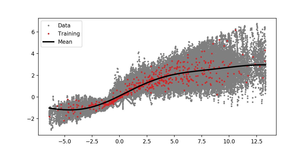
Figure 10: Mean of Gaussian process regression as a closure. Function $c_{\scriptscriptstyle{GP}}$, and data used to determine it, from data generated by (15) with parameters as in (17) and $F_{x}=10.0$

\begin{overpic}[width=260.17464pt]{forecast_gpr40k_periodic_e128.pdf} \put(8.0,37.0){\footnotesize Periodic} \put(100.0,34.0){\fcolorbox{black}{white}{\parbox{1.6cm}{\scriptsize{\color{gray} \bf--} Trajectory \\ {\color{blue} \bf--} Prediction\\ {\color{orange} \bf$\cdot$-} GP closure }}} \end{overpic}

\begin{overpic}[width=260.17464pt]{forecast_gpr40k_quasiperiodic_e128.pdf} \put(8.0,37.0){\footnotesize Quasiperiodic} \end{overpic}

\begin{overpic}[width=260.17464pt]{forecast_gpr40k_slow_e128.pdf} \put(50.0,-2.0){$\tau$} \put(8.0,37.0){\footnotesize Chaotic} \end{overpic}

Figure 11: Comparison of data-driven and model-data-driven prediction The true trajectory is shown in grey, the KAF data-driven prediction in blue and the model-data-driven predictions based on (18) in dotted-red; the periodic, quasiperiodic, and chaotic regimes are considered in turn.

Explicit details of the procedure we use to build a GP closure are described in Appendix B; here we observe that for training we use tuples $\left\{x_{k}(t_{n}),(By)_{k}(t_{n})\right\}_{n=1}^{N}$, over all $k=1,\cdots,9.$ See Figure 10 to see the data used (red random subsamples, without replacement, of the total grey data set), and an approximate GP closure $c_{\scriptscriptstyle{GP}}$ determined from that data.

\begin{overpic}[width=260.17464pt]{NRMSE_L96_p} \put(8.0,37.0){\footnotesize Periodic} \end{overpic}

\begin{overpic}[width=260.17464pt]{NRMSE_L96_qp} \put(8.0,37.0){\footnotesize Quasiperiodic} \end{overpic}

\begin{overpic}[width=260.17464pt]{NRMSE_L96_chaotic} \put(50.0,-2.0){$\tau$} \put(8.0,37.0){\footnotesize Chaotic} \end{overpic}

Figure 12: RMSE comparison for the four cases a)–d) described in the text, in the periodic, quasiperiodic, and chaotic regimes. In the periodic regime, KAF (a) is an ideal predictor with negligible growth in error (note the logarithmic scale). In the quasiperiodic response regime, the growth in RMSE with KAF (a,b) is significantly slower than that of the GP-based ODE prediction (c). In the chaotic response regime, the GP-based ODE prediction (c) is more accurate in the near term, yet KAF error stabilizes as the prediction converges to the conditional mean.

Once we have the closed model appearing in (18) we may use it to predict the variable $x$ appearing in (15), and we may compare that prediction with the one made by KAF. Figure 11 shows the result of doing so. It shows that the KAF approach is superior in the periodic and quasi-periodic settings, but that for predictions of the trajectory itself the model-data based predictor (18) is superior to KAF in the chaotic case. Note that the model-data based predictor has access to more data than does the KAF, and requires model knowledge; the KAF is entirely data-driven.

We now dig a little deeper into the comparison. We do this in a systematic way in the periodic, quasi-periodic and chaotic regimes. In each of these three cases we show four RMSE error curves, labelled as follows: a) the standard KAF based on $x$ data alone; b) an enhanced KAF using $(x,By)$ data, the same data used to train the ODE (18); c) a prediction using the ODE (18); d) a KAF prediction trained on $X$ data alone, generated by the ODE (18). Figure 12 shows that KAF a) is the ideal predictor in the periodic regime and is near-ideal in the quasi-periodic regime; on the other hand the ODE (18) predictor c) is ideal for short-term predictability in the chaotic case. Augmenting observations with $By$ within KAF, as in b), gives errors similar to those arising from a), when observing $x$ alone; thus knowledge of $By$ provides little extra information. In the chaotic case, the RMSE s of KAF trained on $x$, a), and on $X$, d), are very close, confirming that the ODE (18) for $X$ captures the invariant measure of the approximately Markovian variables $x$ as intended.

We emphasize the difference between averaging and homogenization here: in the averaging case observing the fast variables adds nothing to our prediction because there is a closed system determined only by the slow variables (see Figure 12, graphs a) and b) in all three plots). By contrast, in the homogenization case, observing the fast variables improves short-term predictions because it provides further information about the driving stochastic process entering the homogenized limit (see Figure 6).

\begin{overpic}[width=260.17464pt]{forecast40k_chaotic_e1_lsmooth.pdf} \put(40.0,37.0){\footnotesize${\color[rgb]{0,0,0}\Pi}(\omega)=x$} \put(100.0,33.0){\fcolorbox{black}{white}{\parbox{2.3cm}{\scriptsize{\color{gray} \bf--} Trajectory \\ {\color{blue} \bf--} Prediction\\ {\color{pink}$\blacksquare$} Predicted 2$\sigma$ }}} \end{overpic}

Figure 13: Prediction in non-Markovian regime, $F_{x}=10,~{}\varepsilon=1$, results in much shorter accurate trajectory predictability, followed by rapid convergence of the conditional mean to a constant. Note, however, that the uncertainty prediction bands contain the true trajectory for all time.

\begin{overpic}[width=151.76964pt]{{lorenz_l96_40k_periodic_e128_idx1_1.3736}.pdf} \put(30.0,82.0){\footnotesize$x_{1}(0)=1.3736$} \put(48.0,-2.0){$\tau$} \end{overpic}

\begin{overpic}[width=151.76964pt]{{lorenz_l96_40k_periodic_e128_idx1_1.3799}.pdf} \put(30.0,82.0){\footnotesize$x_{1}(0)=1.3799$} \put(-15.0,92.0){\fcolorbox{black}{white}{\footnotesize$\ix(\omega) = x_1$}} \put(48.0,-2.0){$\tau$} \put(90.0,73.0){\fcolorbox{black}{white}{\parbox{2.55cm}{\scriptsize{\color{gray} \bf--} Trajectory \\ {\color{red} \bf...} Lorenz' method \\ {\color{blue} \bf- -} KAF prediction \\ {\color{pink}$\blacksquare$} KAF Predicted 2$\sigma$ }}} \end{overpic}

Figure 14: Lorenz’ method (2) sensitivity to initial conditions, in the partially-observed periodic $F_{x}=5,\varepsilon^{-1}=128$ regime, results in diverging predicted trajectories for nearby initial conditions, separated only by 0.006. By contrast, KAF, which is continuous with respect to initial condition, shows moderate predictive skill and makes nearly identical predictions for nearby initial conditions.

4.4 Non-Markovian regime

In the preceding subsections we studied predictors for $x$, based only on time-series data in the $x$ coordinate, for the equation (15). We studied the scale-separated regime where $\varepsilon\ll 1$ and $x$ is approximately Markovian and deterministic – it is approximately governed by an ODE. Here we study the behavior of identical predictors when $\varepsilon=1$; the system  (15) then no longer exhibits averaging and $x$ is no longer Markovian because there is no scale-separation between $x$ and $y$. This experiment is conducted with $F_{x}=10$. Because of the lack of Markovian behaviour we expect rapid loss of predictability in time, when ${\color[rgb]{0,0,0}\Pi}(\omega)=x,F(\omega)=x_{1}$. The resulting conditional mean and variance, shown in Figure 13, confirms this intuition. Indeed the conditional mean is out of phase with the truth at lead time $\tau=1$, and this is also reflected in the large growth of the conditional variance. Furthermore, the conditional mean tapers to a constant at $\tau=6$, twice as quickly as it does in the $\varepsilon\ll 1$ setting in which this tapering occurs at $\tau\approx 11$ (Figures 8,11).

4.5 Comparison with Lorenz’ method

We illustrate the advantage of KAF over Lorenz’ original method of analog forecasting (2), which can produce predictions that are discontinuous with respect to initial condition. In particular, this occurs when data are partially observed from a larger state space, and different states map to identical partial observations. To study this, we observe a single coordinate $x_{1}$ of the periodic regime ($F_{x}=5,\varepsilon^{-1}=128$) so that the observed data are highly non-Markovian. We select initial conditions that are $\mathcal{O}(10^{-3})$ apart, but are separated in time by integer multiples of the period. Figure 14 plots the resulting predictions from Lorenz’ method and KAF. Although Lorenz’ method is accurate for one initial condition (right), it gives a diverging prediction for a nearly identical point (left). By contrast, KAF is continuous with respect to initial condition and displays theoretically optimal predictive skill (in an RMSE sense) for even highly non-Markovian observation data. This experiment illuminates a key feature of KAF: that it gives consistent predictions that are continuous with respect to initial conditions. Note, also, that KAF uncertainty predictions of a periodic observable are also periodic, and vanish at every half period when predictions intersect the ground truth.

5 Conclusions

1. We have studied KAF for data-driven prediction:

   • we use multi-scale systems to create dynamical systems in which a subset of the variables (slow variables) evolve in an approximately Markovian fashion;

   • we study KAF performance for a range of systems in which the slow variables are governed approximately by stochastic, chaotic, quasi-periodic and periodic behaviour;

   • in the stochastic case we use the homogenized equations for the slow variables to obtain explicit formulae for the eigenfunctions of the operator underlying KAF, and use these to validate the performance of the KAF method;

   • in the chaotic, quasi-periodic and periodic cases we use the averaged equations for the slow variables to obtain a GPR-based approximate closure model, and use hybrid data-model predictions, from this closure, in order to evaluate the KAF method.

2. What we illustrate about use of the KAF:

   • when the variable being predicted is (approximately) a component of a stochastic Markov process then prediction of individual trajectories is not possible, whilst the mean and variance, averaged over possible realizations of the stochastic behaviour, can be accurately predicted by KAF;

   • when the variable being predicted is (approximately) a component of a deterministic but chaotic Markov process then prediction of individual trajectories is also not possible, except over short time horizons;

   • in both the chaotic and stochastic cases, whilst prediction of individual trajectories is not to be expected, simply bounding the future trajectory may be useful in applications – to this end we show that in all cases two standard deviation bands around the predicted conditional mean always reliably capture the truth;

   • in both the stochastic and chaotic settings a signature of the lack of predictability is the convergence of the predictor to a constant, for large $\tau$, accompanied by the data-driven choice of parameter $\ell$ converging to one;

   • when the variable being predicted is (approximately) a component of a deterministic quasi-periodic or periodic process the prediction of individual trajectories over long time horizons is possible; in this case parameter $\ell$ stays away from one, for significantly large $\tau;$

   • in all cases the predicted standard deviations around the predictor provide a reliable indicator of the time-scale on which the predictor is accurate trajectory-wise, and on longer time-scales provide a reliable indicator of the scale of the errors incurred, trajectory-wise;

   • the choice of kernel, and the interpretation of eigenfunctions as harmonics over the observed submanifold, is well-adapted to capturing periodic or quasi-periodic structure whilst the design of eigenfunctions to include the constant eigenfunction permits convergence to the conditional mean for chaotic, mixing dynamics;

   • the choice of $\ell$ indicates the number of harmonics contained in the predicted variable and is often approximately constant in $\tau$ in periodic and quasi-periodic settings, whilst it converges to one in the chaotic or stochastic mixing cases;

   • when the variable being observed does not evolve in an approximately Markovian fashion then the KAF conditional mean cannot track $x$ for even short times, as observed for $\varepsilon=1$ for both the Lorenz 63 and Lorenz 96 examples.

3. The work also suggests a number of directions for future study in the area of KAF:

   • delay embedding can be used to deal with non-Markovian behaviour and it would be of interest to automate the choice of delay embedding dimension within the KAF framework, to get closer to Markovianity;

   • combining KAF with data assimilation holds the possibility of greater predictability – for work in this direction see [20] which studies the EnKF with a data-driven model update;

   • it would be of interest to have algorithms to identify slow subspaces, using data living in larger spaces, and hence to conduct KAF using approximately Markovian variables;

   • it would be of interest to extend KAF predictor $Z_{\tau}$ so that it acts on the joint space of initial conditions and key parameters, enabling prediction at as yet unseen parameters.

Acknowledgments: The work of DB and AMS is supported by the generosity of Eric and Wendy Schmidt by recommendation of the Schmidt Futures program, by Earthrise Alliance, Mountain Philanthropies, the Paul G. Allen Family Foundation, and the National Science Foundation (NSF, award AGS1835860). AMS is also supported by NSF (award DMS-1818977) and by the Office of Naval Research (award N00014-17-1-2079). DG is grateful to the Department of Computing and Mathematical Sciences at the California Institute of Technology for hospitality and for providing a stimulating environment during a sabbatical, where part of this work was completed. DG is supported by NSF (awards 1842538 and DMS-1854383) and ONR (awards N00014-16-1-2649 and N00014-19-1-242). KM is supported by the NSF Mathematical Sciences Postdoctoral Research Fellowship (award 1803663).

Appendix A Computation

This appendix contains details of the implementation of KAF. Subsection A.1 describes the algorithms for computing the kernel, diffusion eigenbasis, RKHS basis functions and finally, the prediction. Our specific choice of kernel, which endows the RKHS structure, is explained and motivated in subsection A.2. We outline procedures for choosing truncation parameter $\ell$ and approximating the conditional variance of the forecast in subsections A.3 and A.4.

A.1 Linear Algebra

A.1.1 Algorithm 1 (Diffusion eigenbasis)

The starting point of this algorithm is the variable-bandwidth diffusion kernel function ${\kappa}_{\scriptscriptstyle{N}}:\mathcal{X}\times\mathcal{X}\to\mathbb{R}$

$${\kappa}_{\scriptscriptstyle{N}}(x,x^{\prime})=\exp\left(\frac{-|x-x^{\prime}|^{2}}{\epsilon{r}_{\scriptscriptstyle{N}}(x){r}_{\scriptscriptstyle{N}}(x^{\prime})}\right),$$

described further in Appendix A.2. An automatic procedure for estimating the data-dependent bandwidth function ${r}_{\scriptscriptstyle{N}}$ and width $\epsilon$ are given in [6].

• Inputs

  • Training data $x_{0},x_{1},\dots x_{N-1}\in\mathcal{X}$

  • Desired maximum number of eigenvectors $L$

• Outputs

  • Diffusion eigenvectors $\phi_{0},\dots,\phi_{L-1}\in\mathbb{R}^{N}$, stacked in matrix ${\Phi}\in\mathbb{R}^{N\times L}$

  • Diffusion eigenvalues $\lambda_{0},\dots,\lambda_{L-1}\in\mathbb{R}$ in diagonal matrix ${\Lambda}\in\mathbb{R}^{L\times L}$

• Steps

  1. Form the matrix ${K}\in\mathbb{R}^{N\times N}$ with entries $K_{ij}=\kappa_{N}(x_{i},x_{j})/N$.

  2. Compute ${v}_{\scriptscriptstyle{N}},{w}_{\scriptscriptstyle{N}}\in\mathbb{R}^{N}$ using ${v}_{\scriptscriptstyle{N}}={K}\vec{1}$ and ${w}_{\scriptscriptstyle{N}}={K}V^{-1}\vec{1}$, where $V=\mbox{diag}({v}_{\scriptscriptstyle{N}})$.

  3. Form normalized kernel matrix $S=V^{-1}{K}W^{-1/2}$ where $W=\mbox{diag}({w}_{\scriptscriptstyle{N}})$.

  4. Compute $L$ largest singular values $\sigma_{0},\dots,\sigma_{L-1}$ and corresponding left singular vectors $\phi_{0},\dots,\phi_{L-1}$ of $S$. Stack eigenvectors columnwise into $N\times L$ matrix ${\Phi}:=[\phi_{0},\dots,\phi_{L-1}]$ and form $L\times L$ diagonal matrix of eigenvalues ${\Lambda}:=\mbox{diag}(\lambda_{j})$, with $\lambda_{j}:=\sigma_{j}^{2}$.

Remark

Recall that the key idea of KAF is the eigendecomposition of the Markov operator $G$ which can be represented by an $N\times N$ matrix

$$G\phi=\lambda\phi.$$

The matrix $G$ is never explicitly formed, instead we exploit the fact that $G=SS^{T}$, and hence $\phi$ are the left singular vectors of $S$. Thus we bypass the eigendecomposition step with a reduced singular value decomposition (SVD) in step (4). Note that the SVD approach is natural when working with kernels with an explicit factorization $G=SS^{T}$, including the bistochastic kernels described in Appendix A.2. For more general kernels one typically performs direct eigendecomposition of $G$. KAF can also be implemented with non-symmetric kernels satisfying a detailed balance condition making them conjugate to positive-definite kernels; see Section 4.2 in [1] for more details.

A.1.2 Algorithm 2 (RKHS basis functions)

RKHS basis functions are computed using the Nyström extension (7) reproduced below

$$\psi_{j}=\frac{1}{N\lambda_{j}^{1/2}}\sum_{n=0}^{N-1}k(\cdot,x_{n})\phi_{j}(x_{n}),\quad\lambda_{j}>0.$$

• Inputs

  • Out-of-sample data $\hat{x}_{0},\hat{x}_{1},\dots\hat{x}_{\hat{N}-1}\in\mathcal{X}$

  • Diffusion eigenvectors ${\Phi}\in\mathbb{R}^{N\times L}$

  • Diffusion eigenvalues ${\Lambda}\in\mathbb{R}^{L\times L}$

• Outputs

  • RKHS basis ${\Psi}=[\psi_{0},\dots,\psi_{L-1}]$

• Steps

  1. Form matrix $\hat{S}\in\mathbb{R}^{L\times N}$ with entries $\hat{S}_{ij}={\kappa}_{\scriptscriptstyle{N}}(\hat{x}_{i},x_{j})$. Note that this requires another kernel density estimation step to evaluate the sampling density on out-of-sample data.

  2. Compute the RKHS basis matrix ${\Psi}={\Lambda}^{-1/2}\hat{S}{\Phi}/N$. RKHS basis functions (evaluated at the out-of-sample points) are the columns $\psi_{0},\dots,\psi_{L-1}$ of ${\Psi}$.

A.1.3 Algorithm 3 (Predictor)

The final predictor is constructed according to (1), reproduced here for convenience

$$Z_{\tau}(x)=\frac{1}{N}\sum_{n=0}^{N-1}\left(\sum_{j=0}^{\ell(\tau)-1}\frac{\psi_{j}(x)\phi_{j}(x_{n})}{\lambda_{j}^{1/2}}\right)f_{n+q}.$$

• Inputs

  • Lead time $\tau=q\Delta t$

  • Truncation parameter $\ell\leq L$

  • Vector of sampled observable ${f}_{\tau}=[f_{q},\dots,f_{N-1+q}]^{T}$

  • Diffusion eigenvectors ${\Phi}_{\ell}\in\mathbb{R}^{N\times\ell}$ (first $\ell$ columns of ${\Phi}$)

  • Diffusion eigenvalues ${\Lambda}_{\ell}=\mbox{diag}(\lambda_{0},\dots,\lambda_{\ell-1})$

  • RKHS basis ${\Psi}_{\ell}\in\mathbb{R}^{N\times\ell}$ (first $\ell$ columns of ${\Psi}$)

• Output

  • Prediction $Z_{\tau}$ at $\hat{x}_{0},\hat{x}_{1},\dots\hat{x}_{\hat{N}-1}$

• Steps

  1. Form $\ell$-dimensional coefficient vector ${c}:={\Phi}_{\ell}^{T}{f}_{\tau}/N$

  2. Compute ${z}:={\Psi}_{\ell}{\Lambda}_{\ell}^{-1/2}{c}$. Report prediction for $i^{th}$ initial point $Z_{\tau}(\hat{x}_{i}):=z_{i}$.

A.2 Choice of Kernel

Details concerning the kernel choice may be found in section 5 of [1]. Here we briefly summarize the key ideas. Our starting point is the Gaussian kernel

$$\kappa(x,x^{\prime};\epsilon)=\exp\bigl{(}-|x-x^{\prime}|^{2}/\epsilon\bigr{)}$$

where we assume that $\mathcal{X}$ is a subset of $\mathbb{R}^{d}$, $x,x^{\prime}\in\mathcal{X}$ and $|\cdot|$ denotes the Euclidean norm on $\mathbb{R}^{d}.$ Note that this kernel is data-independent. From it we can generalize to a data-dependent kernel defined by [7]

$${\kappa}_{\scriptscriptstyle{N}}(x,x^{\prime}) =\exp\bigl{(}-|x-x^{\prime}|^{2}/({r}_{\scriptscriptstyle{N}}(x){r}_{\scriptscriptstyle{N}}(x^{\prime})\epsilon)\bigr{)},$$

$${r}_{\scriptscriptstyle{N}}(x) ={q}_{\scriptscriptstyle{N}}(x)^{\frac{1}{m}},$$

$${q}_{\scriptscriptstyle{N}}(x) =\frac{1}{(\pi\delta)^{m/2}}\int_{\Omega}\kappa(x,{\color[rgb]{0,0,0}\Pi}(\omega);\delta){\mu}_{\scriptscriptstyle{N}}(d\omega).$$

Here, $\epsilon,\delta$ and $m$ are lengthscale and dimension parameters, respectively, estimated from the data. The role of including $r_{n}$, and hence a variable bandwidth kernel, is to compensate for variations in sampling density across the space. A key conceptual idea underlying the construction of ${q}_{\scriptscriptstyle{N}}$ is that it approximates the Lebesgue density of the measure $\mu$ in the large data limit. Thus the kernel ${\kappa}_{\scriptscriptstyle{N}}$ weights the distance of $x$ and $x^{\prime}$ in a manner which reflects the sampling density of the data.

From ${\kappa}_{\scriptscriptstyle{N}}$ the kernel ${k}_{\scriptscriptstyle{N}}$ is constructed as follows, invoking a second principle which is to design a bistochastic Markov kernel [9]. Doing so ensures that the top eigenvalue of $G$ is $1$ with corresponding eigenvector a constant; then the hypothesis space also contains constants. This is useful for capturing the mean of the predicted quantity $U^{\tau}F$ and, in particular, plays a central role in the large $\tau$ asymptotics for mixing systems. To achieve the Markov property we proceed as follows. First we define

$${v}_{\scriptscriptstyle{N}}(x) =\int_{\Omega}{\kappa}_{\scriptscriptstyle{N}}\bigl{(}x,{\color[rgb]{0,0,0}\Pi}(\omega)\bigr{)}{\mu}_{\scriptscriptstyle{N}}(d\omega),$$

$${w}_{\scriptscriptstyle{N}}(x) =\int_{\Omega}\frac{{\kappa}_{\scriptscriptstyle{N}}\bigl{(}x,{\color[rgb]{0,0,0}\Pi}(\omega)\bigr{)}}{{v}_{\scriptscriptstyle{N}}\bigl{(}{\color[rgb]{0,0,0}\Pi}(\omega)\bigr{)}}{\mu}_{\scriptscriptstyle{N}}(d\omega).$$

Since the above empirically determined quantities only take values at the $N$ sampled points, they are isomorphic to vectors in $\mathbb{R}^{N}$ identified by the same name within Algorithm A.1.1. Finally define

$${k}_{\scriptscriptstyle{N}}(x,x^{\prime})=\int_{\Omega}\frac{{\kappa}_{\scriptscriptstyle{N}}\bigl{(}x,{\color[rgb]{0,0,0}\Pi}(\omega)\bigr{)}{\kappa}_{\scriptscriptstyle{N}}\bigl{(}{\color[rgb]{0,0,0}\Pi}(\omega),x^{\prime}\bigr{)}}{{v}_{\scriptscriptstyle{N}}(x){w}_{\scriptscriptstyle{N}}\bigl{(}{\color[rgb]{0,0,0}\Pi}(\omega)){v}_{\scriptscriptstyle{N}}(x^{\prime})}{\mu}_{\scriptscriptstyle{N}}(d\omega).$$

The operators constructed from the unnormalized and normalized kernels, ${\kappa}_{\scriptscriptstyle{N}}$ and ${k}_{\scriptscriptstyle{N}}$, are likewise represented by $N\times N$ matrices $K$ and $S$, respectively, in Algorithm A.1.1. It may be verified that the Markov property is satisfied and so too are the positivity conditions required for the aforementioned large data convergence result.

A.3 Choice of $\ell$

Recall that the predictor (9) actually corresponds to a family of predictors parameterized by the desired lead time $\tau$ and by the truncation parameter $\ell$. Thus we write $Z_{\tau,\ell}.$ Here we describe how to choose $\ell$ for a fixed lead time $\tau$. In practice, the choice of $\ell$ is determined from the minimizer of the empirical RMSE based on (5), computed from a validation data set with $\tilde{N}$ samples $\hat{x}_{0},\dots,\hat{x}_{\tilde{N}-1}:$

$$\ell=\operatorname*{arg\,min}_{\ell^{\prime}=1,\dots,L}{\sf{{RMSE}}\,}(Z_{\tau,\ell^{\prime}}).$$

A.3.1 Algorithm 4 (Tuning $\ell$)

• Inputs

  • Forecast lead time $\tau=q\Delta t$

  • Validation out-of-sample data $\hat{x}_{0},\dots,\hat{x}_{\tilde{N}-1}\in\mathcal{X}$

  • Ground truth vector of observables $\hat{{f}}_{\tau}=[\hat{f}_{q},\dots,\hat{f}_{\tilde{N}-1+q}]^{T}$

  • Diffusion eigenvectors ${\Phi}$ from Algorithm 1

  • Diffusion eigenvectors ${\Lambda}$ from Algorithm 1

• Outputs

  • Truncation parameter $\ell$

• Steps

  1. Compute RKHS basis functions ${\Psi}_{L}$ using Algorithm 2. Set $R:=\infty$.

  2. for $\ell^{\prime}=1$ to $L$

     1. Compute predictor $Z_{\tau,\ell^{\prime}}(\hat{x}):={z}$ using Algorithm 3.

     2. Compute ${\sf{{RMSE}}\,}_{l^{\prime}}$ for $Z_{\tau,\ell^{\prime}}(\hat{x})$ as ${\sf{{RMSE}}\,}_{\ell^{\prime}}:=\|{z}-\hat{{f}}_{\tau}\|_{2}$.

     3. if ${\sf{{RMSE}}\,}_{\ell^{\prime}}\leq R$ set $\ell=\ell^{\prime}$

  3. Return $\ell$.

This tuning procedure must be carried out for each desired lead time $\tau$.

A.3.2 Long-time behavior of $\ell$

It should be noted that in the presence of mixing or chaotic dynamics, for long lead times $\tau$ the projected subspaces become one-dimensional, i.e., $\ell=1$ and the predictor converges to a constant (this occurs only if the subspace includes the constant eigenfunction from a Markov kernel operator). The weak convergence of the conditional expectation of mixing dynamics to the mean of the observable $F$ is described in [1],

(19) $$\lim_{\tau\rightarrow\infty}\langle g,\operatorname{\mathbb{E}}[U^{\tau}F|{\color[rgb]{0,0,0}\Pi}]-\operatorname{\mathbb{E}}[F]\mathbf{1}_{\Omega}\rangle_{L^{2}_{\mu}}=0,$$

a property that is a direct consequence of a measure-theoretic definition of mixing

(20) $$\lim_{\tau\rightarrow\infty}\langle U^{\tau*}g,h\rangle_{L^{2}_{\mu}}=\operatorname{\mathbb{E}}[g]\operatorname{\mathbb{E}}[h],$$

where the expectations are taken over the invariant measure $\mu$.

A.4 Formula for Variance

The uncertainty associated with the prediction at each lead time can be estimated via the conditional variance,

$$\operatorname{var}[U^{\tau}F|{\color[rgb]{0,0,0}\Pi}]=\operatorname{\mathbb{E}}[(U^{\tau}F-\operatorname{\mathbb{E}}[U^{\tau}F|{\color[rgb]{0,0,0}\Pi}])^{2}|{\color[rgb]{0,0,0}\Pi}]\approx\operatorname{\mathbb{E}}[(U^{\tau}F-Z_{\tau})^{2}|{\color[rgb]{0,0,0}\Pi}].$$

The variance is yet another observable in $L^{2}_{\mu}(\Omega;\mathbb{R})$ that can be evaluated using the same basis functions as the predictor, and, once the predictor is computed, it only remains to compute the expansion coefficients

(21) $$\hat{c}_{j}(\tau)=\langle\phi_{j}\circ{\color[rgb]{0,0,0}\Pi},(U^{\tau}F-Z_{\tau})^{2}\rangle_{L^{2}({\mu}_{\scriptscriptstyle{N}})}=\frac{1}{N}\sum_{n=0}^{N-1}\phi_{j}(x_{n})(f_{n+q}-Z_{\tau}(x_{n}))^{2}.$$

Note that this computation requires a different optimal truncation $\ell(\tau)$ for the variance, and hence, another validation set for parameter tuning:

1. (Tuning $\ell$) Run Algorithm 4 on a separate validation data set for which the predictor is already computed, using the new observable $\hat{g}_{\tau}$ instead of $\hat{f}_{\tau}$

   $$\hat{g}_{\tau}=[(\hat{f}_{q}-Z_{\tau}(\hat{x}_{0}))^{2},\dots,(\hat{f}_{\tilde{N}-1+q}-Z_{\tau}(\hat{x}_{\tilde{N}-1}))^{2}]^{T}.$$

2. Run Algorithm 3 on the initial prediction data using the observable $g_{\tau}$ instead of $f_{\tau}$

   $$g_{\tau}=[(f_{q}-Z_{\tau}(x_{0}))^{2},\dots,(f_{N-1+q}-Z_{\tau}(x_{N-1}))^{2}]^{T},$$

   denoting the output predicted variance as $V_{\tau}$.

3. Finally, the uncertainty bands of the predictor at each lead time are given by two standard deviations, or twice the square root of the variance, $Z_{\tau}\pm 2\sqrt{|V_{\tau}|}$.

Appendix B Details Of The GP Closure

In this section we describe details of the construction of the Gaussian process (GP) underlying the model-data-driven approach, and leading to the approximate closed equation (18). We use L-96 explicitly, but the methodology easily generalizes to other multiscale systems.

Construction of a GP closure is performed using the following steps:

1. choose random initial conditions for L-96;

2. numerically integrate for time $T_{\text{conv}}$ to determine an initial condition on the global attractor;

3. numerically integrate from this initial condition with a fixed time-step $\Delta t$ for time $T_{\text{learn}}$ to collect pairs of data:

   $$\left\{\bigg{(}x_{k}(t_{n}),(By)_{k}(t_{n})\bigg{)}\right\}_{n=1}^{N},$$

   for $k=1,\dots,9$, and where $t_{n}=n\Delta t$, $N=\left\lfloor\dfrac{T_{\text{learn}}}{\Delta t}\right\rfloor$;

4. train a GP using collected pairs of data, including optimization over hyperparameters such as lengthscale, and set $c_{\scriptscriptstyle{GP}}$ to be the mean of this GP.

Note that in step (c) we exploit the statistical invariance w.r.t. circular index shifting; this enables us to collect $K$ pairs in one time-step. For numerical implementation of the GPR, we used the scikit-learn package [39]; the kernel of the GP was chosen as the sum of a standard radial basis function, and white noise kernels, setting the noise level in the latter to $0.5$; the length scale was optimized over. Out of roughly $30000$ points obtained in step (c), we subsampled $500$ uniformly at random, without replacement, to train the GP. The result of such a procedure is shown in Fig. 10.

References

- [1] R. Alexander and D. Giannakis, Operator-theoretic framework for forecasting nonlinear time series with kernel analog techniques, Phys. D, (2020), https://doi.org/10.1016/j.physd.2020.132520. In press.
- [2] H. Arbabi and I. Mezic, Ergodic theory, dynamic mode decomposition, and computation of spectral properties of the koopman operator, SIAM Journal on Applied Dynamical Systems, 16 (2017), pp. 2096–2126.
- [3] N. Aronszajn, Theory of reproducing kernels, Transactions of the American mathematical society, 68 (1950), pp. 337–404.
- [4] M. Belkin and P. Niyogi, Laplacian eigenmaps for dimensionality reduction and data representation, Neural computation, 15 (2003), pp. 1373–1396.
- [5] A. Bensoussan, J.-L. Lions, and G. Papanicolaou, Asymptotic analysis for periodic structures, vol. 374, American Mathematical Soc., 2011.
- [6] T. Berry, D. Giannakis, and J. Harlim, Nonparametric forecasting of low-dimensional dynamical systems, Physical Review E, 91 (2015), p. 032915.
- [7] T. Berry and J. Harlim, Variable bandwidth diffusion kernels, Appl. Comput. Harmon. Anal., 40 (2016), pp. 68–96, https://doi.org/10.1016/j.acha.2015.01.001.
- [8] A. Chattopadhyay, E. Nabizadeh, and P. Hassanzadeh, Analog forecasting of extreme-causing weather patterns using deep learning, Journal of Advances in Modeling Earth Systems, 12 (2020), p. e2019MS001958, https://doi.org/10.1029/2019MS001958.
- [9] R. Coifman and M. Hirn, Bi-stochastic kernels via asymmetric affinity functions, Appl. Comput. Harmon. Anal., 35 (2013), pp. 177–180, https://doi.org/10.1016/j.acha.2013.01.001.
- [10] R. R. Coifman and S. Lafon, Diffusion maps, Applied and computational harmonic analysis, 21 (2006), pp. 5–30.
- [11] R. R. Coifman and S. Lafon, Geometric harmonics: a novel tool for multiscale out-of-sample extension of empirical functions, Applied and Computational Harmonic Analysis, 21 (2006), pp. 31–52.
- [12] S. Das and D. Giannakis, Delay-coordinate maps and the spectra of Koopman operators, J. Stat. Phys., 175 (2019), pp. 1107–1145, https://doi.org/10.1007/s10955-019-02272-w.
- [13] L. Delle Monache, F. A. Eckel, D. L. Rife, B. Nagarajan, and K. Searight, Probabilistic weather prediction with an analog ensemble, Monthly Weather Review, 141 (2013), pp. 3498–3516.
- [14] M. Dellnitz and O. Junge, On the approximation of complicated dynamical behavior, SIAM J. Numer. Anal., 36 (1999), p. 491, https://doi.org/10.1137/S0036142996313002.
- [15] I. Fatkullin and E. Vanden-Eijnden, A computational strategy for multiscale systems with applications to lorenz 96 model, Journal of Computational Physics, 200 (2004), pp. 605–638.
- [16] D. Giannakis, Data-driven spectral decomposition and forecasting of ergodic dynamical systems, Appl. Comput. Harmon. Anal., 62 (2019), pp. 338–396, https://doi.org/10.1016/j.acha.2017.09.001.
- [17] D. Giannakis, S. Das, and J. Slawinska, Reproducing kernel hilbert space compactification of unitary evolution groups, arXiv preprint arXiv:1808.01515, (2018).
- [18] D. Giannakis, A. Kolchinskaya, D. Krasnov, and J. Schumacher, Koopman analysis of the long-term evolution in a turbulent convection cell, J. Fluid Mech., 847 (2018), pp. 735–767, https://doi.org/10.1017/jfm.2018.297.
- [19] D. Givon, R. Kupferman, and A. Stuart, Extracting macroscopic dynamics: model problems and algorithms, Nonlinearity, 17 (2004), p. R55.
- [20] F. Hamilton, T. Berry, and T. Sauer, Ensemble kalman filtering without a model, Physical Review X, 6 (2016), p. 011021.
- [21] J. Harlim, S. W. Jiang, S. Liang, and H. Yang, Machine learning for prediction with missing dynamics, arXiv preprint arXiv:1910.05861, (2019).
- [22] S. W. Jiang and J. Harlim, Modeling of missing dynamical systems: Deriving parametric models using a nonparametric framework, 2019, https://arxiv.org/abs/1905.08082.
- [23] D. Kelly and I. Melbourne, Deterministic homogenization for fast–slow systems with chaotic noise, Journal of Functional Analysis, 272 (2017), pp. 4063–4102.
- [24] D. Kelly, I. Melbourne, et al., Smooth approximation of stochastic differential equations, The Annals of Probability, 44 (2016), pp. 479–520.
- [25] M. A. Khodkar, P. Hassanzadeh, and A. Antoulas, A koopman-based framework for forecasting the spatiotemporal evolution of chaotic dynamics with nonlinearities modeled as exogenous forcings, arXiv preprint arXiv:1909.00076, (2019).
- [26] S. Klus, F. Nüske, P. Koltai, H. Wu, I. Kevrekidis, C. Schütte, and F. Noé, Data-driven model reduction and transfer operator approximation, Journal of Nonlinear Science, 28 (2018), pp. 985–1010.
- [27] B. O. Koopman, Hamiltonian systems and transformation in hilbert space, Proceedings of the national academy of sciences of the united states of america, 17 (1931), p. 315.
- [28] M. Korda, M. Putinar, and I. Mezić, Data-driven spectral analysis of the Koopman operator, Appl. Comput. Harmon. Anal., (2018), https://doi.org/10.1016/j.acha.2018.08.002. In press.
- [29] E. N. Lorenz, Deterministic nonperiodic flow, Journal of the atmospheric sciences, 20 (1963), pp. 130–141.
- [30] E. N. Lorenz, Atmospheric predictability as revealed by naturally occurring analogues, Journal of the Atmospheric sciences, 26 (1969), pp. 636–646.
- [31] E. N. Lorenz, Predictability: A problem partly solved, in Proc. Seminar on predictability, vol. 1, 1996.
- [32] I. Melbourne and M. Nicol, Almost sure invariance principle for nonuniformly hyperbolic systems, Communications in mathematical physics, 260 (2005), pp. 131–146.
- [33] I. Melbourne and A. Stuart, A note on diffusion limits of chaotic skew-product flows, Nonlinearity, 24 (2011), p. 1361.
- [34] I. Mezić, Spectral properties of dynamical systems, model reduction and decompositions, Nonlinear Dyn., 41 (2005), pp. 309–325, https://doi.org/10.1007/s11071-005-2824-x.
- [35] I. Mezić, Analysis of fluid flows via spectral properties of the koopman operator, Annual Review of Fluid Mechanics, 45 (2013), pp. 357–378.
- [36] B. Nadler, S. Lafon, R. R. Coifman, and I. G. Kevrekidis, Diffusion maps, spectral clustering and reaction coordinates of dynamical systems, Applied and Computational Harmonic Analysis, 21 (2006), pp. 113–127.
- [37] G. C. Papanicolaou and W. Kohler, Asymptotic theory of mixing stochastic ordinary differential equations, Communications on Pure and Applied Mathematics, 27 (1974), pp. 641–668.
- [38] G. Pavliotis and A. Stuart, Multiscale methods: averaging and homogenization, Springer Science & Business Media, 2008.
- [39] F. Pedregosa, G. Varoquaux, A. Gramfort, V. Michel, B. Thirion, O. Grisel, M. Blondel, P. Prettenhofer, R. Weiss, V. Dubourg, J. Vanderplas, A. Passos, D. Cournapeau, M. Brucher, M. Perrot, and E. Duchesnay, Scikit-learn: Machine learning in Python, Journal of Machine Learning Research, 12 (2011), pp. 2825–2830.
- [40] C. E. Rasmussen and C. K. I. Williams, Gaussian Processes for Machine Learning (Adaptive Computation and Machine Learning), The MIT Press, 2005.
- [41] C. W. Rowley, I. Mezić, S. Bagheri, P. Schlatter, and D. S. Henningson, Spectral analysis of nonlinear flows, Journal of fluid mechanics, 641 (2009), pp. 115–127.
- [42] P. J. Schmid, Dynamic mode decomposition of numerical and experimental data, Journal of fluid mechanics, 656 (2010), pp. 5–28.
- [43] B. Schölkopf, A. Smola, and K. Müller, Nonlinear component analysis as a kernel eigenvalue problem, Neural Comput., 10 (1998), pp. 1299–1319, https://doi.org/10.1162/089976698300017467.
- [44] B. Schölkopf, A. J. Smola, F. Bach, et al., Learning with kernels: support vector machines, regularization, optimization, and beyond, MIT press, 2002.
- [45] A. Singer, From graph to manifold laplacian: The convergence rate, Applied and Computational Harmonic Analysis, 21 (2006), pp. 128–134.
- [46] J. Slawinska and D. Giannakis, Indo-Pacific variability on seasonal to multidecadal time scales. Part I: Intrinsic SST modes in models and observations, J. Climate, 30 (2017), pp. 5265–5294, https://doi.org/10.1175/JCLI-D-16-0176.1.
- [47] N. G. Trillos, M. Gerlach, M. Hein, and D. Slepčev, Error estimates for spectral convergence of the graph Laplacian on random geometric graphs towards the Laplace–Beltrami operator, Found. Comput. Math., (2019), https://doi.org/10.1007/s10208-019-09436-w. In press.
- [48] W. Tucker, The lorenz attractor exists, Comptes Rendus de l’Académie des Sciences-Series I-Mathematics, 328 (1999), pp. 1197–1202.
- [49] H. Van den Dool, A new look at weather forecasting through analogues, Monthly weather review, 117 (1989), pp. 2230–2247.
- [50] U. Von Luxburg, M. Belkin, and O. Bousquet, Consistency of spectral clustering, The Annals of Statistics, (2008), pp. 555–586.
- [51] G. Wahba, Spline models for observational data, vol. 59, Siam, 1990.
- [52] X. Wang, J. Slawinska, and D. Giannakis, Extended-range statistical ENSO prediction through operator-theoretic techniques for nonlinear dynamics, Sci. Rep., 10 (2020), p. 2636, https://doi.org/10.1038/s41598-020-59128-7.
- [53] E. Weinan, Principles of multiscale modeling, Cambridge University Press, 2011.
- [54] D. S. Wilks, Effects of stochastic parametrizations in the lorenz ’96 system, Quarterly Journal of the Royal Meteorological Society, 131 (2005), pp. 389–407, https://doi.org/10.1256/qj.04.03, https://rmets.onlinelibrary.wiley.com/doi/abs/10.1256/qj.04.03, https://arxiv.org/abs/https://rmets.onlinelibrary.wiley.com/doi/pdf/10.1256/qj.04.03.
- [55] Z. Zhao and D. Giannakis, Analog forecasting with dynamics-adapted kernels, Nonlinearity, 29 (2016), p. 2888.