Quantum chaos in a system with high degree of symmetries

Abstract

We study dynamical signatures of quantum chaos in one of the most relevant models in many-body quantum mechanics, the Bose-Hubbard model, whose high degree of symmetries yields a large number of invariant subspaces and degenerate energy levels. While the standard procedure to reveal signatures of quantum chaos requires classifying the energy levels according to their symmetries, we show that this classification is not necessary to obtain manifestation of spectral correlations in the temporal evolution of the survival probability. Our findings exhibit the survival probability as a powerful tool to detect the presence of quantum chaos, avoiding the experimental and theoretical challenges associated with the determination of a complete set of energy eigenstates and their symmetry classification.

I Introduction

Symmetries play an important role in the description of physical systems, helping to simplify their description and temporal evolution. In classical dynamics they are useful to find the coordinates providing the simplest description, in the many-body quantum domain they allow to divide the Hilbert space in unconnected subspaces, strongly reducing the dimensionality of the problem. Systems with symmetries are far more likely to have degenerate energy levels than those without them vonNeuman(1929) ; Reichl(2013) .

Quantum chaos refers to the quantum description of classically chaotic systems, their universal properties associated with Random Matrix Theory, and the presence of the former in systems with no classical analogs Reichl(2013) ; stockmann(2006) ; Gutzwiller(2013) . The best stablished signatures of quantum chaos are its spectral statistics, which require the classification of the states by their symmetry properties Berry(1977) ; Bohigas(1984) ; Percival(1973) . In systems with many symmetries, this process can be very demanding on the theoretical side, and very difficult to implement in experimental studies. For example in the Bose-Hubbard model (BHM), which is the system that we analyze here, the number of symmetry subspaces is at least as large as the number of sites in the lattice.

The BHM is the simplest description of a set of spin-less bosons with interactions in a lattice. It was the first strongly correlated lattice model being realized with ultracold atoms and in which a quantum phase transitions was observed Greiner(2002) . Due to the high degree of controllability and new observational tools, which enable the detection of each individual atom, the model is employed to describe experiments related to quantum simulation, quantum thermalization and in recent years to quantum virtual cooling Bakr(2009) ; Bakr(2010) ; Islam(2015) ; Kaufman(2016) ; Lukin(2019) ; Cotler(2019) .

The spectral properties associated with quantum chaos in the BHM were studied by Kolovsky and Buchleitner Kolovsky(2004) . Lubasch studied measures to explore the relation between quantum chaos and entanglement Lubasch(2009) . A semiclassical analysis connected with Bloch oscillations was presented in Kolovsky2016 . Recently the out-of-time-order correlator and the Lyapunov exponent have been studied in the model Shen(2017) and the statistical distance between initially similar number distributions has been proposed as a reliable measure to distinguish regular from chaotic behavior in a Bose-Hubbard dimer Kidd(2019) .

In the present work, we use the survival probability, a dynamical observable, to identify quantum chaos in the BHM. The survival probability is the probability to find the system in its initial state at time $t$. In chaotic systems, it exhibits a correlation hole of universal character at long times, a dip below the saturation value reached at longer times which can be described analytically employing the two-level form factor of Random Matrix Theory Alhassid(1992) . This observable has been successfully employed in recent works as a quantum chaos indicator in spin systems Torres-Herrera(2017) ; Torres-Herrera(2017-2) ; Torres(2018) ; Torres-Herrera(2019) ; Schiulaz(2019) and in atom-photon systems Lerma-Hernandez(2019) .

Here we show that, contrary to spectral statistics where the signatures of quantum chaos disappear when many symmetry sectors are considered together, in the survival probability the correlation hole manifests even if the whole set of symmetry sectors are included in the dynamics. For a single symmetry sector, signatures of quantum chaos are obtained both in the distribution of unfolded nearest neighbour energy differences and in the survival probability. However, when all the symmetry sectors are considered, the distribution of energy differences changes from Wigner-Dyson to Poisson, whereas the correlation hole in the survival probability is still clearly seen. Analytical expressions are provided, which, besides giving theoretical support to the persistence of the correlation hole, describe the complete evolution of the survival probability, both in the case of one and several symmetry subspaces.

The temporal evolution of the survival probability is naturally fuzzy due to quantum fluctuations, whose relative size compared with their average value do not diminish with the dimension of the system, they are not self-averaging at any scale Torres-Herrera(2019) ; Torres-Herrera(2019-2) . For this reason ensemble averages over an energy window are required to make the correlation hole visible Lerma-Hernandez(2019) . Recently it has been shown that such ensemble of initial states can be prepared in a band of energy eigenstates and allowed to evolve Yang(2020) . This development could facilitate the experimental observation of the correlation hole.

The structure of the paper is as follows. In Sec. II we describe the BHM, its symmetries and the properties of its energy spectrum. Then we describe the dynamics of the survival probability and the correlation hole in Sec. III, both in the case of one symmetry sector and when the whole set of invariant subspaces is considered together. In Sec. IV, the analytical expressions derived in the previous section are shown to describe properly numerical results for the BHM in a chaotic regime. The way these signatures of quantum chaos disappear as we move to integrable limits is also discussed. To finish, our conclusions are given in Sec. V .

II The Bose-Hubbard Model

The model which we consider is the one dimensional BHM with periodic boundary conditions. This model describes the dynamics of $N$ spin-less bosons on a lattice with $L$ sites in a ring array. The Hamiltonian of this system, with $\hbar=1$, is

$$\hat{H}=-J\sum_{l=1}^{L}\left(\hat{a}^{\dagger}_{l+1}\hat{a}_{l}+h.c.\right)+\frac{U}{2}\sum_{l=1}^{L}\hat{n}_{l}\left(\hat{n}_{l}-1\right).$$ (1)

The operators $\hat{a}^{\dagger}_{l}$ and $\hat{a}_{l}$ are the creation and annihilation operators of one boson on the site $l$, respectively. Due to periodic boundary conditions, the index $L+1$ in the first sum should be considered as $L+1:=1$. The first term is the kinetic energy, describing the coherent tunneling between adjacent sites with rate $J$. The second term describes the interaction energy on-site with intensity $U$, where $\hat{n}_{l}=\hat{a}_{l}^{\dagger}\hat{a}_{l}$ gives the number of particles on site $l$ and the total number of particles is constant, $\sum_{l=1}^{L}\hat{n}_{l}=N$.

One of the most relevant aspects of the system is that in the thermodynamic limit it presents a second order quantum phase transition, going from a Mott insulator to a superfluid phase Fisher1989 ; Greiner(2002) ; Cucchietti2007 .

II.1 Symmetries and degenerated subspaces

The symmetries of the BHM are described by the dihedrical group $D_{L}$, which is the group of symmetries of a regular polygon with $L$ sides. One of the symmetries is related to the translational invariance of the Hamiltonian due to the periodic boundary conditions. The shift operator $\hat{S}$ is the responsible of the decomposition into different $\kappa$-subspaces and acts in a Fock state as

$$\hat{S}\ket{n_{1},n_{2},...,n_{L-1},n_{L}}=\ket{n_{L},n_{1},n_{2},...,n_{L-1}}.$$ (2)

The eigenvalues of $\hat{S}$ are $a_{j}=e^{i\kappa_{j}}$ with $\kappa_{j}=2\pi j/L$, the single particle quasimomentum and $j=1,2,...,L$ Kolovsky2016 . The only other symmetry is the parity, which is defined as

$$\hat{\mathcal{P}}\ket{n_{1},n_{2},...,n_{L-1},n_{L}}=\ket{n_{L},n_{L-1},...,n_{2},n_{1}}.$$ (3)

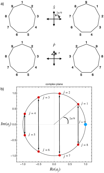
Figure 1: a) Schematic representations of the shift $\hat{S}$ and parity $\hat{\mathcal{P}}$ operators. These operators describe the symmetries of the BH model with periodic boundary conditions and are the same as those of a regular polygon of $L$ sides. b) Eigenvalues of $\hat{S}$ in the complex plane, for $L=9$ sites, indicated by red dots. Pairwise subspaces related by complex conjugate eigenvalues of $\hat{S}$ have the same spectrum, these are linked by the black arrows. The subspace $j=9$ is the only non degenerate subspace and it has two parity symmetric invariant subspaces.

The shift and the parity operators commutes with the BH Hamiltonian (1). However $[\hat{S},\hat{\mathcal{P}}]\neq 0$, which entails a pairwise degenerate spectrum between states belonging to the subspaces with eigenvalues $a_{j}$ and $a_{j}^{*}=a_{L-j}$. For $a_{j=L}=1$ or $a_{j=L/2}=-1$ (the latter appearing only for $L$ even) the subspaces can be decomposed in two additional subspaces with definite parity. In this way we can classify the entire Hamiltonian spectrum.

Fig. 1 a) shows a schematic representation of the shift and parity operator acting on a system of $L=9$ sites. From now on, we consider this number of sites and the same number of bosons $N=9$. For this choice, the Hilbert space dimension is $\mathcal{D}=24310$, and it can be decomposed into $9$ subspaces associated with the eigenvalues $a_{j}$ of $\hat{S}$ as is shown in the Fig. 1 b). The dimensions of the subspaces are $\mathcal{D}_{1}=\mathcal{D}_{8}=2700$, $\mathcal{D}_{2}=\mathcal{D}_{7}=2700$, $\mathcal{D}_{3}=\mathcal{D}_{6}=2703$ , $\mathcal{D}_{4}=\mathcal{D}_{5}=2700$, $\mathcal{D}_{9}=2704$. Additionally, the subspace associated with $j=9$ can be decomposed in two subspaces with definite parity, whose dimensions are $\mathcal{D}_{9-even}=1387$ and $\mathcal{D}_{9-odd}=1317$. In Fig. 1 b) each subspace pair related by the black arrow has the same spectrum. Only the 9-subspace has no degeneracies, and the two subspaces with different parity have different spectrum. This is the full decomposition of the system in symmetries.

For the Hamiltonian parameters, we use the parametrization introduced in Kolovsky(2003) $U=u$ and $J=1-u$ with $u\in[0,1]$. With this parametrization the system is integrable in the two limits $u=0$ and $u=1$. Except for some few indicated cases, in the following sections we use the value $u=0.5$ as a representative chaotic example.

II.2 Level statistics and density of states

We obtained the full spectrum of the model by exact numerical diagonalization. The density of states (DoS) $\nu(E)$ is shown in the Fig. 2 a). The DoS has a Gaussian form, consistent with the finite size of the system. Due to the similar dimension of the subspaces the density of states in each one is very close to a ninth of the total density of states $\nu_{j}(E)=\nu(E)/9$, for $j=1,...,9$. The light gray zone in Fig. 2 a) depicts the energy interval that we consider in the numerical calculations presented below for the spectral distributions and the survival probability. This is a window of width equal to four (energy units) with center in the maximum of the distribution.

The nearest-neighbor spacing distribution for the unfolded energy levels of the 1-subspace, containing the central 80 % of its spectrum, is shown in Fig. 2 b). The red-dashed line is the Wigner-Dyson distribution for the Gaussian orthogonal ensemble (GOE). We have verified the same very good match with the Wigner-Dyson distribution for the energy spacing of the other symmetry subspaces.

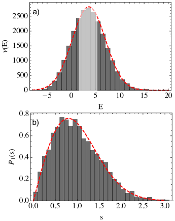
Figure 2: a) Gray bars depict the Density of states (DoS) obtained numerically for the BHM with $L=9$ sites and $N=9$ bosons. A Gaussian fit is shown by the red dashed line. The light-gray zone in the DoS represents the energy interval used in panel (b) and Figs.3, 4 and 7(top). b) Nearest neighbour level spacing distribution for the unfolded spectrum of the subspace associated to $j=1$ ($\kappa_{1}=2\pi/9$) symmetry subspace. The distribution coincides with the Wigner-Dyson surmise of the GOE ensemble (dashed red line).

If we consider the energy levels of all the symmetry sectors contained in the same energy interval as before, we obtain the unfolded energy spacing distribution displayed in the inset of Fig. 3. The distribution shows a peak at zero energy, which comes from the exact respective degeneracies between subspaces 1-4 and 8-5. If we remove these exact degeneracies by considering only subspaces 1-4 and 9, we get rid of the peak and obtain a distribution very close to a Poisson distribution of uncorrelated levels, as can be seen in the main panel of Fig. 3. This well known result shows that the nearest neighbour distribution is unable to capture the intra-correlations between levels of the same symmetry sectors, which become hidden by the lack of correlations between levels of different symmetries.

As we show below, this is not the case of the survival probability, which is sensitive to the correlations in the spectrum even if several symmetry sectors are considered together. In what follows we discuss how these correlations manifests as a dip in the temporal evolution of the survival probability, known as correlation hole, and compare it with the spectral analysis performed above.

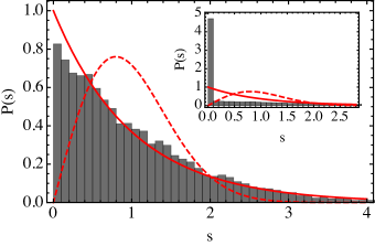
Figure 3: Main panel shows the nearest neighbor spacing distribution of energy levels in the light gray region of Fig.2 considering subspaces $j=1-4$ and $j=9$. Inset shows the same distribution for the whole set of symmetry subspaces.

III The Survival probability and the correlation hole

The survival probability is a dynamical observable defined as the probability to find a given initial state $\ket{\Psi(0)}$ at time $t$,

$$S_{P}(t)=\left|\braket{\Psi(0)}{\Psi(t)}\right|^{2}.$$ (4)

If we expand the initial state $\ket{\Psi(0)}$ in the energy eigenbasis $\{\ket{\phi_{k}}\}$,

$$\ket{\Psi(0)}=\sum_{k=1}^{\mathcal{D}}c_{k}\ket{\phi_{k}},$$ (5)

where $\hat{H}_{BH}\ket{\phi_{k}}=E_{k}\ket{\phi_{k}}$ and $c_{k}=\braket{\phi_{k}}{\Psi(0)}$, the survival probability reads

$$S_{P}(t)=\left|\sum_{k}|c_{k}|^{2}e^{-iE_{k}t}\right|^{2}.$$ (6)

III.1 Initial decay and asymptotic value

The survival probability can be expressed as the squared modulus of the Fourier transform of the local density of states (LDOS)

$$S_{P}(t)=\left|\int\mathcal{G}(E)e^{-iEt}dE\right|^{2}.$$ (7)

where the LDOS, $\mathcal{G}(E)=\sum_{k}|c_{k}|^{2}\delta(E-E_{k})$, is the energy distribution weighted by the components of the initial state. By considering a smoothed approximation to the LDOS, $\rho(E)\approx\mathcal{G}(E)$, we can obtain an analytical expression for the initial decay of $S_{P}(t)$ Torres-Herrera(2017) ; Lerma-Hernandez(2019) . For instance, for a rectangular smoothed profile

$$\rho(E)=\left\{\begin{array}[]{lr}\frac{1}{2\sigma_{R}}&\text{for }E\in[E_{c}-\sigma_{R},E_{c}+\sigma_{R}]\\ 0&\text{otherwise}\end{array}\right.,$$ (8)

we obtain a $sinc$ squared function for the initial decay of $S_{P}(t)$

$$S_{p}^{bc}(t)=\frac{\sin^{2}(\sigma_{R}t)}{(\sigma_{R}t)^{2}},$$ (9)

where the super-index $bc$ indicates that this expression is valid before the dynamics is able to resolve the correlations in the spectrum. In the following, we consider a such rectangular energy profile with parameters determined by the energy window of Fig. 2, where $E_{c}=3.60$ is the center of the distribution and $\sigma_{R}=2$ is its half-width.

The initial decay holds up to a temporal scale where the dynamics is able to resolve the discrete nature of the energy spectrum. For $t\rightarrow\infty$, the survival probability fluctuates around an asymptotic value, $S_{P}^{\infty}$, which can be determined as follows. By expanding the squared modulus in Eq.(4), we obtain

$$S_{P}(t)=\sum_{k\neq l}|c_{l}|^{2}|c_{k}|^{2}e^{-i(E_{k}-E_{l})t}+\sum_{k}|c_{k}|^{4}.$$ (10)

The asymptotic value can be obtained by considering a temporal average of this expression

$$S_{P}^{\infty}=\lim_{t\to\infty}\frac{1}{t}\int_{0}^{\infty}S_{P}(t^{\prime})dt^{\prime}.$$ (11)

In the absence of degeneracies, the first term in the RHS of Eq.(10) cancels out in average and

$$S_{P}^{\infty}=\sum_{k}|c_{k}|^{4},$$ (12)

which is the case of the BHM when only one symmetry sector is considered. In the case of degeneracies, that appear in the BHM when several symmetry sectors are considered, the first term in the RHS of Eq.(10) contributes with extra terms to the asymptotic value, which is now given by

$$S_{P}^{\infty}=\sum_{E_{k}}\left(\sum_{m=1}^{d_{E_{k}}}\left|c_{E_{k},m}\right|^{2}\right)^{2},$$ (13)

where $c_{E_{k},m}$ is the component of the initial state in the energy level $|E_{k},m\rangle$ with degeneracy $d_{E_{k}}$,

$$c_{E_{k},m}=\langle E_{k};m|\Psi(0)\rangle\ \ \ \ (m=1,...,d_{E_{k}}).$$

III.2 Initial states

In between the initial decay and the saturation of the dynamics, correlations in the energy spectrum manifest as a dip of the $S_{P}$ below the asymptotic value. To reveal the presence of this correlation hole, averages over different initial states have to be considered Torres-Herrera(2017) ; Torres-Herrera(2017-2) ; Torres(2018) ; Torres-Herrera(2019) ; Schiulaz(2019) ; Lerma-Hernandez(2019) . In this paper we consider ensembles of initial states with components different to zero only in the energy interval $[E_{c}-\sigma_{R},E_{c}+\sigma_{R}]$ and whose squared modulus are randomly chosen as follows

$$|c_{k}|^{2}=\frac{r_{k}f(E_{k})}{\sum_{q}r_{q}f(E_{q})},$$ (14)

where $r_{k}\in[0,1]$ are random numbers coming from a uniform distribution. The function $f(E)=\rho(E)/\nu(E)$ guarantees that the random initial state has the selected energy profile $\rho(E)$. This is achieved by compensating, with the denominator, for changes in the density of states.

III.3 Analytical expressions for the survival probability

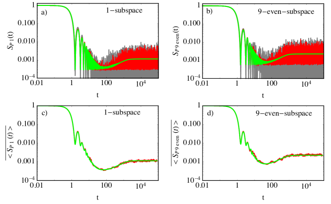
Figure 4: Survival probability as a function of time in log-log scale. Panels a) and b) show, for subspace $j=1$ and $j=9$-even respectively, the survival probability for individual members of the ensemble (gray lines), dark red lines represent the ensemble averages and light green lines are obtained from the analytical expression (15). A similar behavior (not shown) was found for the rest of symmetry subspaces. Panel c) and d) show averages over temporal windows of constant size in log scale plotted versus the mean time of the respective temporal windows for the numerical ensemble average of $S_{P}(t)$ (dark red) and for the analytical expression of the survival probability (light green). Panel c) is for the 1-subspace and panel d) for the 9-even-subspace.

III.3.1 One symmetry sector

In Lerma-Hernandez(2019) , by following an idea initially introduced in Herrera(2018) , an analytical expression for the ensemble average of the survival probability was derived, which applies for the case of one sequence of non-degenerate energy levels with energy density $\nu$ and correlations similar to those of random matrices of a Gaussian orthogonal ensemble (GOE)

$$\braket{S_{P}(t)}=\frac{1-\langle S_{P}^{\infty}\rangle}{\eta-1}\left[\eta S_{P}^{bc}(t)-b_{2}\left(\frac{t}{2\pi\bar{\nu}}\right)\right]+\langle S_{P}^{\infty}\rangle,$$ (15)

here $S_{P}^{bc}(t)$ is given in Eq.(9), $\bar{\nu}$ is the mean DoS in the energy interval, and $\eta$ is the effective dimension of energy levels available for the ensemble, which is given by

$$\eta=\frac{1}{\int dE\frac{\rho^{2}(E)}{\nu(E)}}=\frac{4\sigma_{R}^{2}}{\int_{E_{c}-\sigma_{R}}^{E_{c}+\sigma_{R}}dE\frac{1}{\nu(E)}},$$ (16)

where in the last equality we have used the rectangular profile for the energy distribution. When the energy interval is approximately centered in the middle of the Gaussian distribution for $\nu(E)$, the last equation can be approximated by substituting $\nu(E)$ in the denominator by its average in the energy interval ($\bar{\nu}$), leading to a simple expression

$$\eta=2\sigma_{r}\bar{\nu},$$

which equals the number of states in the energy interval. The asymptotic value $\braket{S_{P}^{\infty}}$ is obtained by averaging expression (12), which can be shown Lerma-Hernandez(2019) to be given by

$$\braket{S_{P}^{\infty}}=\frac{\braket{r^{2}}}{\braket{r}^{2}}\frac{1}{\eta}=\frac{4}{3\eta},$$ (17)

where $\braket{r^{n}}$ is the n-th moment of the distribution of the random numbers and in the last equality we have used that for an uniform distribution $\langle r^{n}\rangle=1/(n+1)$.

The second term inside the brackets in Eq. (15) is the two-level form factor of the GOE ensemble (Alhassid(1992), ),

$$\begin{split}b_{2}(t)&=\left[1-2t+t\ln(2t+1)\right]\Theta(1-t)\\ &+\left[t\ln\left(\frac{2t+1}{2t-1}\right)-1\right]\Theta(t-1),\end{split}$$ (18)

where $\Theta$ is the Heaviside step function. The two-level form factor brings the survival probability from its minimum value up to the asymptotic value $\braket{S_{P}^{\infty}}$, creating the dip that is known as the correlation hole. Although the averaged survival probability can display oscillations, the presence of a hole which can be described by (15) is a direct signature of the existence of correlated eigenvalues, and it does not develop in systems with uncorrelated eigenvalues.

III.3.2 Whole set of symmetry sectors

The formula (15) is applicable to the BHM when only one symmetry sector is considered. Here we extend Eq.(15) to the case where the whole set of symmetry sectors are included. The general formulae and details of the derivation can be seen in the Appendix. Here we present the results for random numbers coming from an uniform distribution, and for the BHM with $L=9$ sites and $N_{S}=10$ symmetry sectors whose densities are approximately $\nu_{j}=\nu/9$ for $j=1,...,8$ and $\nu_{9-even}=\nu_{9-odd}=\nu/18$, while their degeneracies are $d_{j}=2$ for $i=1,...,8$ and $d_{9-even}=d_{9-odd}=1$. For this particular case the ensemble average of the survival probability reads

$$\langle S_{P}(t)\rangle_{{}_{\hbox{\scriptsize$a$}}}= \frac{1-\langle S_{P}^{\infty}\rangle_{{}_{\hbox{\scriptsize$a$}}}}{\eta-1}\left[\eta S_{P}^{bc}(t)-\frac{16b_{2}\left(\frac{9t}{2\pi\bar{\nu}}\right)+b_{2}\left(\frac{18t}{2\pi\bar{\nu}}\right)}{9}\right]$$

$$+\langle S_{P}^{\infty}\rangle_{{}_{\hbox{\scriptsize$a$}}},$$ (19)

where the density $\nu(E)$ that has to be considered in Eq.(16) to calculate $\eta$ is the density of the whole spectrum. The asymptotic value of $\braket{S_{P}(t)}_{a}$ is now obtained by ensemble averaging Eq.(13), which yields

$$\langle S_{P}^{\infty}\rangle_{{}_{\hbox{\scriptsize$a$}}}=\frac{4}{3\eta}+\frac{8}{9}\frac{\left(1-\frac{4}{3\eta}\right)}{\eta-1}\xrightarrow{\eta\gg 1}\frac{20}{9\eta}.$$ (20)

The key point is that, again, as in the case of only one symmetry sector, the intra-correlations of levels in the same symmetry sectors, brings the survival from its minimum up to the asymptotic value, creating a correlation hole.

At variance with the one-symmetry case, in this case the correlation hole is governed by a pair of two-level form-factors $b_{2}$. One coming from the subspaces 1-8 which implies that the density entering in its argument is $\bar{\nu}_{j}=\bar{\nu}/9$, while the second comes from intra-correlations in the spectrum of subspaces $9$-even and $9$-odd. That is why in the argument of this $b_{2}$ function enters $\bar{\nu}_{9-\text{even}}=\bar{\nu}_{9-\text{odd}}=\bar{\nu}/18$. Since the dynamics of subspaces 1-8 have the same temporal scale, their individual contributions add coherently to build up the correlation hole and they dominate the second term inside the parenthesis in (19).

IV Numerical vs analytical results

In this section we compare the analytical expressions for the survival probability from the previous section with numerical results obtained by diagonalizing numerically the BHM for one and the whole set of symmetry sectors. We also study the way as the signatures of chaos, i.e. the correlation hole, dilutes as we approach an integrable limit.

IV.1 Correlation hole for an ensemble of initial states in the same symmetry subspace

In Fig. 4 we compare numerical results for the survival probability with the analytical expression given by Eq. (15). We employ the same distribution of random initial states in the energy interval $[E_{c}-\sigma,E_{c}+\sigma]$ indicated by light-gray columns at the center of the DoS in Figure 2. For each $\kappa_{j}$ subspace, we consider as many random initial states as the number of energy levels of that subspace in the energy interval, i.e, $\sim 1170$ for the $j=1-4$-subspaces and $\sim 590$ initial states for the subspaces 9-even and 9-odd. The exact numbers are shown in the third column of Table 1.

In Fig. 4 (a) and (b), the gray lines show the survival probability as a function of time for different random initial states with components in the indicated $\kappa_{j}$-subspace, the red lines are the numerical averages over the ensemble, whereas the green line is the analytic expression given in Eq. (15) with parameters determined from Eqs.(16) and (17). We can see that the analytical expression properly describes the temporal trend of the numerical ensemble average. At short times and before the $S_{P}(t)$ attains its minimum value, the fluctuations of the numerical ensemble average are small, which is a consequence of the fact that the initial decay is determined entirely by the smoothed energy profile of the initial states, Eq. (9), which is the same for every member of the ensemble. At the temporal scale of the correlation hole and beyond, the fluctuations in the numerical ensemble average are relatively larger. To further reduce these fluctuations we consider averages over temporal windows of constant size in log scale. By considering the same smoothing procedure in the analytical expression, we obtain Figures 4 (c) and (d), which show an excellent agreement between the analytical expression and numerical averages, and make evident the correlation hole, confirming the existence of a GOE correlated spectrum and thus quantum chaos in this energy region of the Bose-Hubbard model.

IV.1.1 Survival probability for different regions of the spectrum

$\overline{\braket{S_{P}(t)}}$
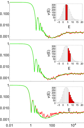
	$t$

Figure 5: Averages over temporal window of constant size in log scale of the numerical ensemble average of the Survival probability, plotted versus the mean value of the respective temporal windows (red dark line). Three ensembles over energy regions with $600$ levels each were considered. The energy regions of each ensemble are indicated in the histograms shown as insets. Light green lines indicate the same temporal averages of the analytical expression (15). Only energy levels of the $j=1$-subspace were considered. From top to bottom the energy regions move from the center of the spectrum to its highest border.

In the previous section we have analyzed initial states with random components in the central region of the spectrum. Now we study what happens with the survival probability if we select initial states in energy regions approaching the border of the spectrum. It is known that the universal statistical properties of the chaotic spectra are not applicable to the borders of the spectra, which are model dependentGutzwiller(2013) . This is confirmed in the behavior of the survival probability shown in Fig.5 with dark red lines. Results for three ensembles are shown, one ensemble, as before and used as reference, is located in the center of the DoS and the other two approach the high energy border of the spectrum. We consider again rectangular energy profiles, and move the energy window to the large energy regions using eigenstates of the 1-subspace. The energy windows we consider are shown in the insets of Fig. 5. The number of energy levels contained in the three energy windows is equal to $600$.

We observe, as in Fig.4, a correlation hole for the first and second ensemble of states, located respectively in the central part of the spectrum and in a region with slightly higher energies. In both cases the survival probability and correlation hole are very well described by the analytical expression (15), shown with light green lines. Since these two ensembles prove energy levels far enough of the borders of the spectrum, the universal behavior expected from the GOE ensemble is clearly observed.

For the third ensemble, located close to the border of the spectrum, we can observe a clear deviation respect to the universal behavior indicated by the light green line obtained from Eq.(15). We observe a correlation hole in the numerical results that is smaller than the one coming from the analytical expression. This implies that, contrary to the two previous ensembles, only a fraction of levels in this energy region have GOE correlations. The participation, in this third ensemble, of energy levels located in the higher part of the spectrum, not only diminish the depth of the correlation hole, but also produce larger oscillations in the survival probability, as can be observed in the bottom panel of Fig.4.

IV.1.2 Survival probability for different Hamiltonian parameters

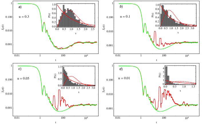
Figure 6: Averages over temporal windows of the survival probability for initial states with components in the central part of the spectrum of the 1-subspace. The dark red curve is the numerical ensemble average of the survival probability, while the light green line is the analytical expression (15). Four different couplings $u$, indicated in each panel, were used. The insets display the corresponding nearest neighbor spacing distribution, where the continuous red line is the Poisson distribution and the dashed line is the Wigner-Dyson distribution.

Above we have analyzed the properties of the spectrum of the BHM in the chaotic regime with parameter $u=0.5$. In this section we study the survival probability with initial states in the same central region of the spectrum of the symmetry sector $\kappa_{1}$, but now for values of the parameter $u$ approaching the integrable limit $u=0$.

In Fig 6 we show the combined ensemble and temporal average of the survival probability, both numerical (red) and analytical (green), for four different values of the $u$ parameter. For $u=0.3$ Fig. 6 a) shows a perfect match between numerical and analytical results and a clear presence of the correlation hole. This is consistent with the nearest neighbor energy distribution shown in the inset, which is very well described by the Wigner-Dyson surmise. As we approach the integrable limit, the nearest neighbor energy differences histograms in the insets of Figs.(b,c,d) show that the spectrum correlations disappear. Accordingly, except for the initial decay and asymptotic value, the analytical expression no longer describes the numerical survival probability and instead of a correlation hole we observe revivals whose amplitude increases as the value of $u$ approaches the integrable limit.

IV.2 Correlation hole for an ensemble of initial states in the full space

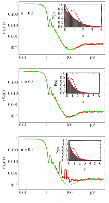
Figure 7: Dark red lines show the temporal mean of the survival probability for the ensemble average of 10581 initial states with the same number of components inside the central energy interval of all the symmetry subspaces. Three different couplings $u$, indicated in each panel, were employed. For the top panel the energy interval used is indicated by light-gray bars in panel a) of Fig. 2. Light green lines are the temporal mean of the analytical expression in Eq.(19). Insets show the corresponding nearest neighbor spacing distribution of energy levels considering only subspaces $j=1-4$ and $j=9$.

In this section we present numerical and analytical results for random initial states but considering now the whole set of symmetry sectors. The combined temporal and ensemble average of $S_{P}(t)$ for a such set of initial states with the participation of levels in the energy interval indicated by light-gray bars in Fig.2 is shown with a red line in Fig 7(top). The important finding is that, even if we employ the complete energy spectrum without any consideration about symmetries, the survival probability exhibits a clearly visible correlation hole, which is again very well described by the analytical expression (green line), now given by Eq. (19), whose parameters are determined from Eqs. (16) and (20).

By inspecting Eq.(19), we observe that the correlation hole is governed mainly by the first term with the two-level form factor $b_{2}$ coming from the subspaces $\kappa_{j}=\kappa_{1},...,\kappa_{8}$, which is $16$ times larger than the second term with the $b_{2}$ function coming from the subspaces $9$-even and $9$-odd. The presence of $(L-2)/2$ (for even $L$) or $(L-1)/2$ (for odd $L$) sequences of energy levels with similar densities and GOE intra-correlations, is the general scenario that can be found in the BHM for an arbitrary number of sites, and therefore no-exception can be foreseen for the appearance of the correlation hole in the chaotic regime of the BHM for arbitrary size. To illustrate the generality of the previous scenario, we show in Fig. 7(middle) the same analysis as before, but now for a coupling $u=0.3$. We observe a perfect match between analytical and numerical results, allowing to conclude that this coupling corresponds also to a chaotic regime.

Finally, in the bottom panel of Fig.7 we present the survival probability for a coupling, $u=0.1$, close to the integrable limit. Similarly to the results shown in Fig.6(b,c,d), only the initial decay and asymptotic value are well described by the analytical expression. At the temporal scale where the correlation hole would develop, the numerical results show instead partial revivals, indicating that for this coupling there are no GOE correlations even for states belonging to the same symmetry sector.

Fig.7 shows that for an spectrum coming from different symmetry sectors, the correlation hole in the survival probability serves as a good indicator of quantum chaos, differently to the nearest-neighbour-energy differences distribution, which, as shown in the insets of Fig.7, are Poisson-like in the three cases and thus useless to distinguish a chaotic from a regular regime.

Even in more general chaotic cases, distinct to the BHM, the analytical general formula for the ensemble average of $S_{P}$ presented in the Appendix, shows that the correlation hole is a general feature appearing in the evolution of the $S_{P}(t)$ and can be used as a reliable indicator of quantum chaos without having to classify the energy levels according to their symmetries. In this context, it is appropriate to mention a recent study of the temporal evolution of the Survival Probability in the chaotic region of the Dicke model Villasenor2020 , where initial states mixing two subspaces with different parity symmetries are considered. In that reference is also reported the need to employ the full effective dimension $\eta$, but only the density of states of every subspace to describe analytically the presence of the correlation hole in the numerical averages. This result is a particular case of the general formula described in the Appendix for the survival probability when several symmetry subspaces are included.

$\kappa_{j}$-subspace	$\braket{S_{P}^{\infty}}\times 10^{3}$	$\eta$	$\overline{\nu}$
1, 8	1.11	1174	293.5
2, 7	1.13	1175	293.7
3, 6	1.13	1178	294.5
4, 5	1.13	1179	294.7
9 even	2.23	597	149.25
9 odd	2.32	574	143.5
Complete	0.210	10581	2645.25

Table 1: Parameters of the analytical equation (15) plotted in Fig.4 for the $j=1,9$-subspaces. Second and third column come, respectively, from equations (17) and (16). Last row shows the parameters used in the analytical expression (19) plotted in the top panel of Fig.7. Second and third-column values come from eqs.(20) and (16). For the cases shown the parameter $\eta$ coincides with the respective number of states in the energy window shown by light gray columns in Fig.2.

V Conclusions

In the present work we have studied dynamical signatures of quantum chaos in the Bose-Hubbard model in a ring configuration. After exhibiting that, when levels in the same subspace of the shift symmetry are considered, the unfolded nearest neighbor distribution match the Wigner-Dyson surmise of the Gaussian orthogonal ensemble; we have shown that this is not the case when the full spectrum is included: when the energy degeneracies are removed from the whole spectrum, the distribution becomes Poisson-like. Then, we have studied the ensemble average of the Survival Probabililty $\braket{S_{p}(t)}$ for initial states in each symmetry subspace and located in different energy windows. We have shown that, when the energy window is located far from the border of the spectrum, a correlation hole in the survival probability develops in all the subspaces. It was also shown that the complete evolution of the survival probability is very well described by an analytical expression deduced employing Random Matrix Theory. These results exhibit the presence of the correlation hole in the Survival Probability as a clear signature of quantum chaos.

Unlike the well established spectral analysis, we found that the correlation hole is a signature of quantum chaos that does not require the classification of states according to their symmetries. Contrary to the analysis of the nearest-neighbor-energy-differences, in the survival probability the intra-correlations of levels in the same symmetry sectors are not washed out by the absence of correlations between levels coming from different symmetry sectors. Analytical expressions supporting the previous result were given and shown to describe perfectly the numerical results. The existence of the correlation hole was also correlated with the presence of quantum chaos for different values of the interaction u.

The finding that the correlation hole is present even when no separation in symmetries is performed, exhibits the survival probability as a very useful and powerful tool to identify the presence of quantum chaos in systems where the symmetry separation is far from trivial, either in the theoretical analysis or in its experimental observation.

An interesting extension of the studies presented here would be to investigate the dynamics of special sets of initial states, like Fock states. The dependence of the dynamics of the survival probability on the dimension of the systems and the study of other observables would be other interesting directions to be investigated.

VI Acknowledgments

We thank L. Santos and J. Torres for their useful comments. We acknowledge the support of the Computation Center-ICN, in particular to Enrique Palacios, Luciano Díaz and Eduardo Murrieta. Also we acknowledge funding from Mexican Conacyt project CB2015-01/255702, and DGAPA-UNAM projects No. IN109417 and IN104020.

Appendix A Ensemble average of the Survival Probability for several degenerate sequences of energy levels

Here we generalize the analytical expression for the ensemble average of the Survival probability in chaotic regimes derived in Lerma-Hernandez(2019) to the case of several symmetry sectors with energy degeneracies, which is the general case of the Bose-Hubbard model.

Let $N_{e}$ be the number of energy sequences. We assume that the unfolded energies in every sequence have the same correlations as the Gaussian Orthogonal Ensemble, and no correlations exist between energies of different sequences. Let $d_{i}$, $\nu_{i}$ and $L_{i}$ be, respectively, the degree of degeneracy of each energy level, the Density of States and the number of energy levels in the $i$-th energy sequence ($i=1,...,N_{e}$). The following relation holds $\sum_{i}^{N_{e}}d_{i}\nu_{i}=\nu$, where $\nu$ is the Density of States of the whole spectrum. The survival probability can be expressed as

$$SP(t)=\sum_{E_{ik}\not=E_{i^{\prime}k^{\prime}}}\left|c_{ik}^{(m)}\right|^{2}\left|c_{i^{\prime}k^{\prime}}^{(m^{\prime})}\right|^{2}e^{-i(E_{ik}-E_{i^{\prime}k^{\prime}})t}+$$

$$\sum_{i=1}^{N_{E}}\sum_{k=1}^{L_{i}}\left(\sum_{m=1}^{d_{i}}\left|c_{ik}^{(m)}\right|^{2}\right)^{2},$$

where $c_{ik}^{(m)}$ are the energy components of the initial state $|\Psi_{o}\rangle=\sum c_{i,k}^{(m)}|E_{i,k};m\rangle$. The first term in the expression has an infinite temporal average equal to zero and the second term ($S_{P}^{\infty}$) gives the asymptotic value of the survival probability.

As stated in the main text, the components of the initial states are chosen randomly according to

$$\left|c_{ik}^{(m)}\right|^{2}=\frac{r_{ik}^{(m)}f(E_{ik})}{\sum_{i^{\prime}k^{\prime}m^{\prime}}r_{i^{\prime}k^{\prime}}^{(m^{\prime})}f(E_{i^{\prime}k^{\prime}})},$$

where $f(E_{ik})=\rho(E_{ik})/\nu(E_{ik})$ and $r_{ik}^{(m)}$ are positive random numbers from a probability distribution $p(r)$.

To derive an analytical expression for the ensemble average of the Survival probability, we proceed similarly as Lerma-Hernandez(2019) , and consider the following approximations

$$\left\langle\left|c_{ik}^{(m)}\right|^{4}\right\rangle\approx\frac{\langle r^{2}\rangle}{\langle r\rangle^{2}}f_{ik}^{2}$$

and

$$\left\langle\left|c_{ik}^{(m)}\right|^{2}\left|c_{i^{\prime}k^{\prime}}^{(m^{\prime})}\right|^{2}\right\rangle\approx\frac{\eta}{\eta-1}\left(1-\frac{\langle r^{2}\rangle}{\langle r\rangle^{2}}\frac{1}{\eta}\right)f_{ik}f_{i^{\prime}k^{\prime}},$$

where we have used the shorthand notation $f_{ik}=f(E_{ik})$, $\langle r^{n}\rangle$ are the $n$-th moments of the probability distribution $p(r)$ and

$$\eta\equiv\frac{1}{\sum_{ikm}f_{ik}^{2}}\approx\frac{1}{\int\frac{\rho^{2}(E)}{\nu(E)}dE}$$

is the effective dimension of states available for the ensemble.

With the previous approximations and following a similar procedure as Lerma-Hernandez(2019) we obtain the following expression for the ensemble average of the asymptotic value of the survival probability

$$\langle S_{P}^{\infty}\rangle_{a}=\frac{\langle r^{2}\rangle}{\langle r\rangle^{2}}\frac{1}{\eta}+\frac{\left(1-\frac{\langle r^{2}\rangle}{\langle r\rangle^{2}}\frac{1}{\eta}\right)}{\eta-1}\sum_{i=1}^{N_{e}}d_{i}(d_{i}-1)\frac{\nu_{i}}{\nu},$$

whereas for the entire survival probability, we obtain the following expression for the ensemble average

$$\langle S_{P}(t)\rangle_{a}=$$ (21)

$$\frac{\left(1-\langle S_{P}^{\infty}\rangle_{a}\right)}{\eta-1}\left[\eta S_{P}^{bc}(t)-\sum_{i=1}^{N_{e}}d_{i}^{2}\frac{\bar{\nu_{i}}}{\bar{\nu}}b_{2}\left(\frac{t}{2\pi\bar{\nu_{i}}}\right)\right]+\langle S_{P}^{\infty}\rangle_{a},$$

where $S_{P}^{bc}(t)=\left|\int\rho(E)e^{-iEt}\right|^{2}$ gives the initial decay of the survival probability and $\bar{\nu_{i}}$ is the respective mean density of states in the energy window. It is straightforward to show that the previous expression for the survival probability has the right value in $t=0$, $\langle S_{P}(t=0)\rangle_{a}=1$.

For the Bose-Hubbard model we consider in this paper ($L=N=9$), we have 6 sequences of energy levels, four of them have degeneracy two ($d_{1}=d_{2}=d_{3}=d_{4}=2$) and the other two are non degenerate $d_{9-even}=d_{9-odd}=1$. The respective Density of States are $\nu_{1}=\nu_{2}=\nu_{3}=\nu_{4}=\nu/9$ and $\nu_{9-even}=\nu_{9-odd}=\nu/18$. For this case, the ensemble averages read

$$\langle S_{P}^{\infty}\rangle_{a}=\frac{\langle r^{2}\rangle}{\langle r\rangle^{2}}\frac{1}{\eta}+\frac{\left(1-\frac{\langle r^{2}\rangle}{\langle r\rangle^{2}}\frac{1}{\eta}\right)}{\eta-1}\frac{8}{9}$$ (22)

and

$$\langle S_{P}(t)\rangle=\langle S_{P}^{\infty}\rangle_{a}+$$ (23)

$$\frac{\left(1-\langle S_{P}^{\infty}\rangle_{a}\right)}{\eta-1}\left[\eta S_{P}^{bc}(t)-\frac{16}{9}b_{2}\left(\frac{9t}{2\pi\bar{\nu}}\right)-\frac{1}{9}b_{2}\left(\frac{9t}{\pi\bar{\nu}}\right)\right].$$

For the particular uniform distribution $p(r)$ we consider in the main text $\frac{\langle r^{2}\rangle}{\langle r\rangle^{2}}=\frac{4}{3}$, by substituting this ratio in Eqs.(22) and (23) we retrieve Eqs.(19) and (20) of the main text.

References

- (1) J. von Neuman and E. Wigner. Uber merkwürdige diskrete Eigenwerte. Uber das Verhalten von Eigenwerten bei adiabatischen Prozessen. Physikalische Zeitschrift, 30:467–470, Jan 1929.
- (2) Linda Reichl. The transition to chaos: conservative classical systems and quantum manifestations. Springer Science & Business Media, 2013.
- (3) H.J. Stöckmann. Quantum Chaos: An Introduction. Quantum Chaos: An Introduction. Cambridge University Press, 2006.
- (4) Martin C Gutzwiller. Chaos in classical and quantum mechanics, volume 1. Springer Science & Business Media, 2013.
- (5) Michael Victor Berry, M. Tabor, and John Michael Ziman. Level clustering in the regular spectrum. Proceedings of the Royal Society of London. A. Mathematical and Physical Sciences, 356(1686):375–394, 1977.
- (6) O. Bohigas, M. J. Giannoni, and C. Schmit. Characterization of chaotic quantum spectra and universality of level fluctuation laws. Phys. Rev. Lett., 52:1–4, Jan 1984.
- (7) I C Percival. Regular and irregular spectra. Journal of Physics B: Atomic and Molecular Physics, 6(9):L229–L232, sep 1973.
- (8) Markus Greiner, Olaf Mandel, Tilman Esslinger, Theodor W. Hänsch, and Immanuel Bloch. Quantum phase transition from a superfluid to a mott insulator in a gas of ultracold atoms. Nature, 415(6867):39–44, 2002.
- (9) Waseem S. Bakr, Jonathon I. Gillen, Amy Peng, Simon Fölling, and Markus Greiner. A quantum gas microscope for detecting single atoms in a Hubbard-regime optical lattice. Nature, 462(7269):74–77, 2009.
- (10) W. S. Bakr, A. Peng, M. E. Tai, R. Ma, J. Simon, J. I. Gillen, S. Fölling, L. Pollet, and M. Greiner. Probing the superfluid–to–Mott Insulator Transition at the Single-Atom level. Science, 329(5991):547–550, 2010.
- (11) Rajibul Islam, Ruichao Ma, Philipp M. Preiss, M. Eric Tai, Alexander Lukin, Matthew Rispoli, and Markus Greiner. Measuring entanglement entropy in a quantum many-body system. Nature, 528(7580):77–83, 2015.
- (12) Adam M. Kaufman, M. Eric Tai, Alexander Lukin, Matthew Rispoli, Robert Schittko, Philipp M. Preiss, and Markus Greiner. Quantum thermalization through entanglement in an isolated many-body system. Science, 353(6301):794–800, 2016.
- (13) Alexander Lukin, Matthew Rispoli, Robert Schittko, M. Eric Tai, Adam M. Kaufman, Soonwon Choi, Vedika Khemani, Julian Léonard, and Markus Greiner. Probing entanglement in a many-body–localized system. Science, 364(6437):256–260, 2019.
- (14) Jordan Cotler, Soonwon Choi, Alexander Lukin, Hrant Gharibyan, Tarun Grover, M. Eric Tai, Matthew Rispoli, Robert Schittko, Philipp M. Preiss, Adam M. Kaufman, Markus Greiner, Hannes Pichler, and Patrick Hayden. Quantum Virtual Cooling. Phys. Rev. X, 9:031013, Jul 2019.
- (15) A. R Kolovsky and A Buchleitner. Quantum chaos in the Bose-Hubbard model. Europhysics Letters (EPL), 68(5):632–638, dec 2004.
- (16) M Lubasch. Quantum chaos and entanglement in the Bose-Hubbard model. Diploma (Master) thesis, Heidelberg University. See http://www. thphys. uni-heidelberg. de/wimberger/diploma_thesis_lubasch. pdf, 2009.
- (17) Andrey R. Kolovsky. Bose–Hubbard Hamiltonian: Quantum chaos approach. International Journal of Modern Physics B, 30(10):1630009, 2016.
- (18) Huitao Shen, Pengfei Zhang, Ruihua Fan, and Hui Zhai. Out-of-time-order correlation at a quantum phase transition. Phys. Rev. B, 96:054503, Aug 2017.
- (19) R. A. Kidd, M. K. Olsen, and J. F. Corney. Quantum chaos in a Bose-Hubbard dimer with modulated tunneling. Phys. Rev. A, 100:013625, Jul 2019.
- (20) Y. Alhassid and R. D. Levine. Spectral autocorrelation function in the statistical theory of energy levels. Phys. Rev. A, 46:4650–4653, Oct 1992.
- (21) E. J. Torres-Herrera and Lea F. Santos. Extended nonergodic states in disordered many-body quantum systems. Annalen der Physik, 529(7):1600284, 2017.
- (22) E. J. Torres-Herrera and Lea F. Santos. Dynamical manifestations of quantum chaos: correlation hole and bulge. Philosophical Transactions of the Royal Society A: Mathematical, Physical and Engineering Sciences, 375(2108):20160434, 2017.
- (23) E. J. Torres-Herrera, Antonio M. García-García, and Lea F. Santos. Generic dynamical features of quenched interacting quantum systems: Survival probability, density imbalance, and out-of-time-ordered correlator. Phys. Rev. B, 97:060303, Feb 2018.
- (24) Eduardo Jonathan Torres-Herrera and Lea F. Santos. Signatures of chaos and thermalization in the dynamics of many-body quantum systems. The European Physical Journal Special Topics, 227(15):1897–1910, Mar 2019.
- (25) Mauro Schiulaz, E. Jonathan Torres-Herrera, and Lea F. Santos. Thouless and relaxation time scales in many-body quantum systems. Phys. Rev. B, 99:174313, May 2019.
- (26) S. Lerma-Hernández, D. Villaseñor, M. A. Bastarrachea-Magnani, E. J. Torres-Herrera, L. F. Santos, and J. G. Hirsch. Dynamical signatures of quantum chaos and relaxation time scales in a spin-boson system. Phys. Rev. E, 100:012218, Jul 2019.
- (27) E. Jonathan Torres-Herrera, Mauro Schiulaz, Francisco Perez-Bernal, and Lea F. Santos. Self-averaging behavior at the metal-insulator transition of many-body quantum systems out of equilibrium, 2019.
- (28) Dayou Yang, Andrey Grankin, Lukas M. Sieberer, Denis V. Vasilyev, and Peter Zoller. Quantum non-demolition measurement of a many-body Hamiltonian. Nature Communications, 11(1):775, 2020.
- (29) Matthew P. A. Fisher, Peter B. Weichman, G. Grinstein, and Daniel S. Fisher. Boson localization and the superfluid-insulator transition. Phys. Rev. B, 40:546–570, Jul 1989.
- (30) Fernando M. Cucchietti, Bogdan Damski, Jacek Dziarmaga, and Wojciech H. Zurek. Dynamics of the Bose-Hubbard model: Transition from a Mott insulator to a superfluid. Phys. Rev. A, 75:023603, Feb 2007.
- (31) Andrey R. Kolovsky and Andreas Buchleitner. Floquet-Bloch operator for the Bose-Hubbard model with static field. Phys. Rev. E, 68:056213, Nov 2003.
- (32) E. J. Torres-Herrera, Antonio M. García-García, and Lea F. Santos. Generic dynamical features of quenched interacting quantum systems: Survival probability, density imbalance, and out-of-time-ordered correlator. Phys. Rev. B, 97:060303, Feb 2018.
- (33) David Villasenor, Saul Pilatowsky-Cameo, Miguel A Bastarrachea-Magnani, Sergio Lerma-Hernandez, Lea F Santos, and Jorge G Hirsch. Quantum vs classical dynamics in a spin-boson system: manifestations of spectral correlations and scarring. arXiv preprint, 2002.02465, Feb 2020, New Journal of Physics, in press, doi:10.1088/1367-2630/ab8ef8.