Quasi-deterministic dynamics, memory effects, and lack of self-averaging
in the relaxation of quenched ferromagnets

Abstract

We discuss the interplay between the degree of dynamical stochasticity, memory persistence and violation of the self-averaging property in the aging kinetics of quenched ferromagnets. We show that, in general, the longest possible memory effects, which correspond to the slowest possible temporal decay of the correlation function, are accompanied by the largest possible violation of self-averaging and a quasi-deterministic descent into the ergodic components. This phenomenon is observed in different systems, such as the Ising model with long-range interactions, including mean-field, and the short-range random field Ising model.

Introduction — When computing thermodynamic properties one must, in principle, consider the full statistical-mechanical average $\langle\cdot\rangle$, namely over the realisations of the stochastic trajectories, the initial conditions and, if present, over the quenched disorder distribution. However, if the sample has specific self-averaging properties, the latter two averages are not necessary because they are realised by the system itself in the thermodynamic limit. Restricting for the moment the discussion to clean samples, i.e. without quenched disorder, this occurs when the system is ergodic. In this case after some time a large part of phase space is visited, and the memory of the initial condition is fully lost: therefore, the fate of a thermodynamical process does not depend on the specific initial microstate belonging to the same macrostate.

The situation is more subtle when phase space breaks into ergodic components Palmer (1982), namely mutually non-accessible regions. In this case, if the initial state is well inside one of such components its memory cannot be deleted because the other cannot be accessed. This is trivial for a uniaxial ferromagnet below the critical temperature $T_{c}$, where the equilibrium magnetisation $M$ takes the two possible values $M_{\pm}=\pm M_{eq}$. A sample prepared with a macroscopic $M(t=0)>0$ ($<0$) evolves towards the positive (negative) equilibrium value and self-averaging is not operating.

A different situation occurs when the system is initially on the boundary ${\cal B}$ between ergodic components. In ferromagnets, ${\cal B}$ is the set of configurations with $M\simeq 0$, and this happens when the initial state is sampled from a high temperature ($T\geq T_{c}$) equilibrium state. The evolution in this case proceeds by coarsening of domains of the competing equilibrium phases Corberi and Politi (2015), whose typical size $L(t)$, at time $t$, grows unbounded. Aging is manifested  and the dynamics remains on ${\cal B}$ for ever. This is strictly true if the thermodynamic limit is taken before letting time $t$ large. However, in all physical situations, one deals with a large but finite system. Therefore the initial state, due to thermal fluctuations, will have some offset $M(0)$ from ${\cal B}$ and one can ask how this may change the destiny of the system.

The different options can be appreciated in terms of the exponent $\lambda$ controlling the decay of the autocorrelation function and also related Bray and Derrida (1995) to the growth in time of the magnetization $M(t)\sim L(t)^{d-\lambda}$, where $d$ is the spatial dimension. The Fisher-Huse inequality Fisher and Huse (1988); Yeung et al. (1996) fixes the bounds for $\lambda$

$$\frac{d}{2}\leq\lambda\leq d.$$ (1)

If the system stays close to ${\cal B}$ for ever   the magnetization does not amplify ($\lambda=d$), self-averaging is at work, and memory of the initial condition is retained the least possible . In the opposite situation the system deterministically falls in the ergodic component selected by the sign of $M(0)$. In this case the offset $M(0)$ is strongly amplified and $M(t)$ grows as fast as possible, i.e. $\lambda=d/2$. This process is associated to the longest possible memory of the initial condition and to the strongest violation of self-averaging. In between these two extrema there is a continuum of options, with $d/2<\lambda<d$.

Existing analytical Kissner and Bray (1993); Liu and Mazenko (1991); Mazenko (1998); Corberi et al. (2002a) and numerical Lorenz and Janke (2007); Henkel and Pleimling (2003); Abriet and Karevski (2004); Newman et al. (1990); Bray (1990); Liu and Mazenko (1991) determinations of $\lambda$ suggest that the maximum of memory, $\lambda=d/2$, is only approached in unphysical limits, diverging space dimension limit $d\to\infty$ or diverging order parameter components limit ${\cal N}\to\infty$. Instead, upon associating the origin of the lower bound $\lambda=d/2$ to some deterministic properties of the dynamics, in this paper we show that it is possible to toggle among all the three situations above and that the case with $\lambda=d/2$ is found also for finite $d$ and ${\cal N}$ in the presence of long-range interactions or in the presence of quenched disorder.

The model and the two limiting regimes — In order to set the stage with a specific example, let us start our discussion by considering the one-dimensional clean ferromagnet described by the Hamiltonian

$$H=-\frac{1}{2}\sum_{i,j}J(|i-j|)s_{i}s_{j},$$ (2)

where $s_{i}=\pm 1$ are $N$ Ising variables, and $J(r)=\delta_{r,1}$ for nearest neighborgs (nn) couplings, and $J(r)=1/r^{1+\sigma}$ in the case of long-range interactions. We will focus on the case $\sigma>0$ where additivity and extensivity hold Campa et al. (2009). The model has a ferromagnetic phase below a finite critical temperature $T_{c}(\sigma)>0$ for $\sigma<1$ Dyson (1969); Tomita (2009); it has a Kosterlitz-Thouless transition Fröhlich and Spencer (1982) for $\sigma=1$; finally, $T_{c}=0$ for $\sigma>1$.

Let us now discuss the relaxation of the model with a non conserved order parameter after a quench from $T_{i}=\infty$ to a low $T$. We consider Glauber dynamics where a random spin is reversed with probability $w=(1+\exp(\Delta E/T))^{-1}$, where $\Delta E$ is the energy difference due to the spin-flip. Not only the static properties, also the non-equilibrium kinetics change crossing $\sigma=1$. $L(t)\sim t^{1/z}$ grows with a dynamical exponent Bray and Rutenberg (1994); Rutenberg and Bray (1994) $z=1+\sigma$ for $0<\sigma\leq 1$ or $z=2$ for $\sigma>1$ and nn. This behavior is captured by a single domain model. The distance $X(t)$ between two neighbouring domain walls satisfies an overdamped Langevin equation, $\dot{X}(t)=-F(X)+\xi(t)$, where $F(X)$ is a force determined by Eq. (2) and $\xi(t)$ is a gaussian white noise. The force is given by $F(X)=-U^{\prime}(X)$, where $U(X)=\sum_{i=1}^{X}\left(\sum_{j=-\infty}^{0}+\sum_{j=X+1}^{\infty}\right)J(|i-j|)$. For large $X$ we can replace discrete summations with integrals and evaluating the integrals in the brackets we obtain $U(X)\simeq(2/\sigma)\int_{1}^{X}ds/s^{\sigma}$, therefore $F(X)\sim-1/X^{\sigma}$. Given that $F(X)$ is the average speed of the domain wall the closure time of a domain of initial size $X(0)=L$ is $t=\int_{L}^{0}dX/F(X)\propto L^{z}$ with $z=1+\sigma$ for $\sigma\leq 1$ and $z=2$ for $\sigma>1$. The difference between these two regimes is due to the deterministic force $F(X)$, that affects the coarsening process in the former ($\sigma\leq 1$) while it is irrelevant in the latter ($\sigma>1$). For this reason these regimes will be called convective and diffusive regimes, respectively.

These two regimes can be clearly distinguished by considering the fluctuating magnetisation $M(t)=\sum_{i=1}^{N}s_{i}$, which is shown in Fig. 1 for systems prepared with a fixed condition $M(0)$ $\sim\sqrt{N}$ equal for all $\sigma$-values. In the convective regime $M(t)$ asymptotically diverges and it typically has the same sign as $M(0)$ . In the diffusive regime it fluctuates around $M(0)$. This means that the convective regime keeps memory of the initial condition, while the diffusive does not. This implies that decorrelation is slower in the first case and, actually, we will show in a moment that it occurs in the slowest possible way. Self-averaging with respect to initial conditions is broken for $0<\sigma\leq 1$ (convective regime) while it holds for $\sigma>1$ (diffusive regime).

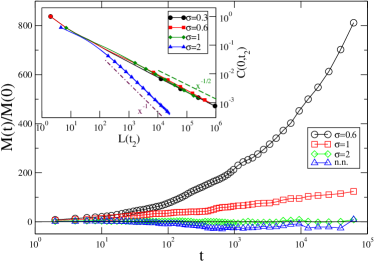
Figure 1: The fluctuating magnetization $M(t)$ for a single realization starting from the same initial condition. The system size is $N=10^{6}$ and the quench temperature is $T=0.1$. In the inset $C(0,t_{2})$ is plotted against $L(t_{2})$ for different $\sigma$ after a quench to $T=0.1$. System size is $N=2\times 10^{7}$. The dashed straight lines are the decays $x^{-\lambda}$ with $\lambda=1$ and $\lambda=1/2$.

With this example in mind, we now turn to a more general discussion. Let us consider the correlation function which, using a continuous picture for a scalar field  $\phi(\mathbf{x},t)$, reads $S(r;t_{1},t_{2})\equiv\langle\phi(\mathbf{x}+\mathbf{r},t_{1})\phi(\mathbf{x},t_{2})\rangle$, where $t_{2}>t_{1}$ and $\langle\cdots\rangle$ is the full non-equilibrium statistical average. We focus on the scaling regime where the autocorrelation function $C(t_{1},t_{2})=S(r=0;t_{1},t_{2})$ behaves as Bray (1994)

$$C(t_{1},t_{2})\simeq\left[L(t_{1})/L(t_{2})\right]^{\lambda},$$ (3)

where, as it will be discussed around Eq. (9), $\lambda$ is the same exponent introduced before which therefore obeys Eq. (1).

The inequalities for $\lambda$ — A derivation of Eq. (1) is now provided following Yeung et al. (1996). We indicate with $u_{l}=\phi_{l}(\mathbf{q},t_{1})$ the Fourier transform of the field $\phi_{l}(\mathbf{x},t_{1})$ evaluated at the time $t_{1}$ during the $l$-th realization of the dynamics. Similarly we define $v_{l}=\phi_{l}(\mathbf{q},t_{2})$ at the time $t_{2}$. We can therefore define the scalar product as $\vec{u}\cdot\vec{v}\equiv(2\tilde{N})^{-1}\sum_{l}(u_{l}v_{l}^{*}+c.c)=\frac{1}{2}\left[S(q,t_{1},t_{2})+S^{*}(q,t_{1},t_{2})\right]$, where $\tilde{N}$ is the number of realizations and $S(q,t_{1},t_{2})\equiv\langle\phi(\mathbf{q},t_{1})\phi(-\mathbf{q},t_{2})\rangle$ is the Fourier transform of $VS(r;t_{1},t_{2})$, $V$ being the system volume. We can now apply the Cauchy-Schwarz inequality, $|\vec{u}\cdot\vec{v}|\leq|u||v|$ and obtain

$$\frac{1}{2}|S(q,t_{1},t_{2})+S^{*}(q,t_{1},t_{2})|\leq\sqrt{S(q,t_{1})S(q,t_{2})},$$ (4)

where, for ease of notation, $S(q,t)\equiv S(q,t,t)$. If we integrate over $\mathbf{q}$ we find

$$C(t_{1},t_{2})\leq\frac{1}{V(2\pi)^{d}}\int d\mathbf{q}\,\sqrt{S(q,t_{1})S(q,t_{2})}.$$ (5)

Using Eq. (3) and the scaling form $S(q,t)=L^{d}(t)f(qL)$, with $f(x)\simeq 1$ for $x\ll 1$ and $f(x)$ negligibly small for $x\gg 1$, we find the lower bound of Eq. (1) .

We now originally prove that the same lower bound can be derived from the term $q=0$ only of Eq. (4),

$$S(0,t_{1},t_{2})\leq\sqrt{S(0,t_{1})S(0,t_{2})}\,.$$ (6)

Using the scaling form for $S(q,t)$ (see below Eq. (5)) it is straightforward to rewrite the previous equation as

$$S(0,t_{1},t_{2})\leq f(0)(L_{1}L_{2})^{d/2},$$ (7)

where we used the shorthand $L_{1}\equiv L(t_{1})$, and similarly for $L_{2}$. The left-hand side of Eq. (5) can be worked out expressing the two-time correlation function as follows, $C(t_{1},t_{2})=\frac{1}{V(2\pi)^{d}}\int d\mathbf{q}\,S(q,t_{1},t_{2})=\frac{L_{2}^{d}}{V(2\pi)^{d}}\int d\mathbf{q}\,F(qL_{2},L_{1}/L_{2}),$ where we have used the scaling hypothesis $S(q,t_{1},t_{2})=L_{2}^{d}F(qL_{2},L_{1}/L_{2})$, valid when both times $t_{1}$ and $t_{2}$ are in the scaling regime. In the limit of large $L_{2}$ (i.e., of large $t_{2}$) only wavevectors $q<1/L_{2}$ contribute to the integral. If $S(q\to 0,t_{1},t_{2})$ goes to a constant, which is the case for quenches below $T_{c}$ or to $T=0$, we can finally write

$$C(t_{1},t_{2})\simeq\frac{1}{V(2\pi)^{d}}\frac{S(0,t_{1},t_{2})}{L_{2}^{d}}.$$ (8)

Using this relation and Eq. (7) we find $C(t_{1},t_{2})\leq\mbox{const}\times(L_{1}/L_{2})^{d/2}$ and the scaling form (3) gives $\lambda\geq d/2$. Therefore Eq. (6) is equivalent to the lower bound (1).

The upper bound in Eq. (1) is defined in Fisher and Huse (1988) as a “suggestive bound” because it cannot be proved as rigorously as the lower bound. In order to derive it, starting from the straightforward relation $\langle M(t_{1})M(t_{2})\rangle=S(0,t_{1},t_{2})$, and using Eqs. (8) and (3), one arrives at

$$\langle M(t_{1})M(t_{2})\rangle=\mbox{const}\times L_{1}^{\lambda}L_{2}^{d-\lambda}.$$ (9)

Authors of Ref. Fisher and Huse (1988) argue that $\lambda\leq d$ because “forgetting of an initial bias appears unlikely”. In other words the strongest memory loss corresponds to the limit $\lambda=d$.

Averaging and memory — We now consider the role of the different statistical averages. The full one $\langle\cdots\rangle$ is taken over the stochastic trajectories, $\langle\cdots\rangle_{tr}$; the initial condition, $\langle\cdots\rangle_{i}$; and, if present, over the quenched disorder, $\langle\cdots\rangle_{q}$. Let us consider, to begin with, a clean system. We can split the fluctuating magnetisation as $M(t)=\langle M(t)\rangle_{tr}+\psi(t)$, where $\psi(t)$ is the stochasticity left over after taking the partial averaging $\langle M(t)\rangle_{tr}$, so that $\langle\psi(t)\rangle_{tr}\equiv 0$. Then we have $\langle M(t_{1})M(t_{2})\rangle=\big{\langle}\langle M(t_{1})\rangle_{tr}\langle M(t_{2})\rangle_{tr}\big{\rangle}_{i}+\big{\langle}\psi(t_{1})\psi(t_{2})\big{\rangle}$. If we now fix $t_{1}$ and let $t_{2}$ diverge, $\langle\psi(t_{1})\psi(t_{2})\rangle=\langle\psi(t_{1})\rangle\langle\psi(t_{2})\rangle=0$ and from Eq. (9) we obtain

$$\big{\langle}\langle M(t_{1})\rangle_{tr}\langle M(t_{2})\rangle_{tr}\,\big{\rangle}_{i}\simeq L_{2}^{d-\lambda}.$$ (10)

Next we argue that, if the quench is made in a ferromagnetic phase, due to the presence of two ergodic components, for large $t_{1}$ it is $\mbox{sign}\big{(}M(t_{1})\big{)}=\mbox{sign}\big{(}M(t_{2})\big{)}$. This is very well observed for $\sigma<1$, see Fig. 1. Hence it is also $\mbox{sign}\langle M(t_{1})\rangle_{tr}=\mbox{sign}\langle M(t_{2})\rangle_{tr}$, therefore Eq. (10) (valid for $t_{1}$ fixed) amounts to

$$\langle M(t)\rangle_{tr}\simeq L(t)^{d-\lambda},$$ (11)

where we have denoted $t_{2}$ as $t$ to ease the notation. Notice that the equation above is more general and applies to systems without a proper ferromagnetic phase, such as the $1d$ Ising model with $\sigma>1$ or with nn, because in this case there is no development of magnetisation starting from a given state, see Fig. 1, and indeed it is $\lambda=d$.

Equation (11) shows that the slowest possible decorrelation, $\lambda=d/2$, is accompanied by the fastest possible growth of the magnetization developed from an initial condition Bray and Derrida (1995). Let us observe that such maximum growth is the one expected upon assuming a random arrangements of a number $\sim VL^{-d}$ of domains of size $L$ each contributing a magnetisation $\sim L^{d}$. Eq. (11) for $\lambda=d/2$ then derives from the central limit theorem.

The result (11) implies also that there is breaking of self-averaging with respect to initial conditions if $\lambda<d$, as reflected by the fact that, for large $N$, the observable magnetisation does not attain its average value $\lim_{N\to\infty}\langle M(t)\rangle=0$ unless the average over initial conditions is performed. The most severe self-averaging breakdown occurs when $\lambda$ is at the lower bound in (1), whilst it is fully restored when it is at the upper bound.

Let us put these arguments to the test in different models, starting from the $1d$ model of Eq. (2). Let us recap what is known about $\lambda$. For nn there is the exact result Glauber (1963) $\lambda=1$, the upper bound of Eq. (1) is saturated and self-averaging holds. For the long-range case it was shown in Corberi et al. (2019a) that there are two universality classes associated to the values $\lambda=1$ (for $\sigma>1$) and $\lambda=1/2$ (for $\sigma\leq 1$). Since it is known Yeung et al. (1996) that for non conserved order parameter this exponent is independent of $t_{1}$, the best determination can be obtained by letting $t_{1}=0$. This is displayed in the inset of Fig. 1, where $C(0,t_{2})$ is shown for various choices of $\sigma$, showing that $\lambda=1$ for $\sigma>1$ and $\lambda=1/2$ for $\sigma\leq 1$.

In Fig. 2 we plot $\langle M(t)\rangle_{tr}$ as a function of $L(t)$, for different $\sigma$ and the same initial condition. This shows very clearly that in the convective regime ($0<\sigma\leq 1$) where $\lambda=d/2$ it is $\langle M(t)\rangle_{tr}\sim\sqrt{L(t)}$ while in the diffusive case ($\sigma>1$ or nn) it is $\langle M(t)\rangle_{tr}\sim M(0)$, as expected after Eq. (11). Hence $\sigma=1$ separates the two opposite situations in which the dynamics occurs on the boundary ${\cal B}$ of the ergodic components (for $\sigma>1$) from the one where it deterministically sinks into such components (for $\sigma\leq 1$). We should stress that $T_{c}=0$ is not a sufficient condition to have $\lambda=d$, as attested by the $2d$ XY-model where $\lambda\simeq 1.17<d=2$ even if $T_{c}=0$ Lee et al. (1995).

In our model (2) determinism can be ascribed to the convective character of domain wall motion Corberi et al. (2019b, a). Let us suppose to have two close domains of sizes $\ell_{1},\ell_{2}$, with $\ell_{2}$ slightly larger than $\ell_{1}$. In the diffusive case the average closure time of $\ell_{1}$, $\overline{t_{1}}$, is slightly smaller than the one of $\ell_{2}$, $\overline{t_{2}}$, but the probability that $t_{1}<t_{2}$ is only slightly larger than $1/2$. In the convective regime, instead, the dominance of the deterministic force makes a domain wall always move towards the closest one Corberi et al. (2019a), so that $t_{1}$ is always smaller than $t_{2}$. This induces a memory effect, since domains which are eliminated have a larger probability to be anti-aligned with $M(t)$ and their removal further increase $M(t)$. Summarising, in the convective regime there is a reduced degree of stochasticity and an increased memory with respect to the diffusive one, and this is the physical origin of the saturation of $\lambda$ to the lower bound.

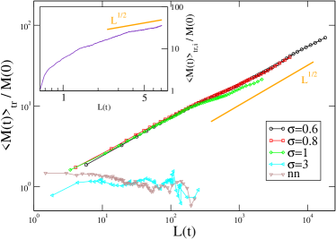
Figure 2: $\langle M(t)\rangle_{tr}$ (normalized by its typical initial value $M(0)$) is plotted against $L(t)$ for different $\sigma$. The system size is $N=10^{6}$ and the quenching temperature is $T=0.1$. The orange straight line is the behavior $L(t)^{1/2}$. In the inset a similar plot is shown for $\langle M(t)\rangle_{tr,i}$ in the $1d$ RFIM quenched to $T\to 0$ with $h/T=1/2$. The system size is $N=10^{5}$.

Same ideas, other models — Let us now apply these ideas to different systems, starting from the short-range ferromagnetic model in $d>1$. In this case we have strict inequalities for any $d$, $d/2<\lambda<d$ Mazenko (1998). Hence self-averaging is spoiled, $\lambda<d$, in opposition to $d=1$. This is because in $d>1$ interfaces do not freely diffuse, there is a deterministic drift induced by the curvature. However the fate of the system is not fully determined by such deterministic force because the shape of the percolating cluster plays a major role in the subsequent dynamics Blanchard, T. et al. (2014). Hence there is only a weak drift from ${\cal B}$ towards the ergodic components and $\lambda$ stays larger than $d/2$.

When long-range interactions are present, results in $d>1$ are rare Christiansen et al. (2019a) and studies of $\lambda$ are almost absent Christiansen et al. (2019b). However it is interesting that for the nn case in the limit $d\to\infty$, which corresponds to the, so to say, longest possible range of interactions, the mean-field, one has $\lambda\to d/2$ Mazenko (1998) and $M(t)\sim L(t)^{d/2}$ Corberi et al. (2017, 2019b), as expected on the basis of our previous argument. In this limit there are no interfaces and, therefore the strong memory effects leading to $\lambda=d/2$ cannot be associated to the determinism of their motion, as in finite dimension. Instead, it can be observed that mean-field amounts to an averaging procedure which makes the evolution, in a sense, more deterministic. Again, this reduction of the stochastic degree is perhaps the physical origin of the saturation of $\lambda$ to the lower bound of Eq. (1).

There is another well known limit in which phase-ordering has a similar character. This is the case of a vectorial order parameter $\vec{\phi}(\mathbf{x},t)$ with a large number ${\cal N}$ of components and short-range interactions. In the ${\cal N}\to\infty$ limit (a model sometimes denoted also as spherical model) one finds Corberi et al. (2002a) $\lambda=d/2$ for any $d$ . By choosing an initially magnetised state it can be shown Zannetti (1993) that the magnetisation evolves deterministically as $M(t)\sim L(t)^{d/2}$, as expected after Eq. (11). It must be recalled that the large-${\cal N}$ limit effectively amounts to replace $\phi^{2}$ with its mean value Corberi et al. (2002a). Then, similarly to mean-field, the model realises a sort of averaging wich tames the stochasticity and sets $\lambda$ to the minimum possible value.

Up to now we have only considered clean systems. It is now interesting to discuss the case with quenched disorder focusing, as a paradigm, on the Random Field Ising Model (RFIM). The RFIM Hamiltonian is given by Eq. (2), plus a contribution $-\sum_{i}h_{i}s_{i}$ due to a quenched random external field that in the following we will consider with zero average and bimodal distribution $h_{i}=\pm h$. We will focus on the nn case. In order to discuss the role of the different averages, as done before, we must now take into account that in this case also the quenched one $\langle\cdots\rangle_{q}$ comes into the game. Splitting the magnetisation as $M(t)=\langle M(t)\rangle_{tr,i}+\psi(t)$, similarly to what done previously for the clean case but where now $\langle\cdots\rangle_{tr,i}$ is a partial average taken over both dynamical trajectories and initial conditions, one can follow the same line of reasoning as before, arriving at the same results, replacing everywhere $\langle M(t)\rangle_{tr}$ with $\langle M(t)\rangle_{tr,i}$.

Let us start discussing the case with $d=1$, for which some analytical arguments are available. The model is characterised Corberi et al. (2002b) by a value of $\lambda$ at its minimum, $\lambda=1/2$. Hence, one should expect $\langle M(t)\rangle_{tr,i}\sim L(t)^{1/2}$. In the inset of Fig. 2 we plot $\langle M(t)\rangle_{tr,i}$ versus the average size of domains $L(t)$ (which grows as $(\ln t)^{2}$). The result nicely confirms our expectation. In this case the growth of $\langle M(t)\rangle_{tr,i}$ can be traced back to the fact that the sum of the random fields in a given quenched realisation is of order $N^{-1/2}$ and, hence, there is an explicit breaking of the up-down spin symmetry. Hence, here it is the random field which causes the deterministic fall into the ergodic components. Interestingly, this effect seems not to be limited to one dimension. For $d>1$ the RFIM can only be studied numerically. For $d=2$ one observes Corberi et al. (2012) that $\lambda=d/2=1$ is still at the lowest possible value, as for $d=1$. This suggests that the mechanism found in $d=1$ might be a general feature with random fields.

Conclusions — We have interpreted the exponent $\lambda$ and its bounds, $d/2\leq\lambda\leq d$, in terms of stochasticity, memory effects, ergodicity breaking and self-averaging. When $\lambda=d$ memory is lost as fast as possible, magnetisation does not develop, and there is no breaking of self-averaging. This occurs, for instance in the $1d$ Ising model with nn, or in the $2d$, ${\cal O}(2)$ model E Nam et al. (2011). When $\lambda=d/2$ memory is maintained as much as possible, magnetization grows as $M(t)\sim(L(t))^{d/2}$ and there is a strong breaking of self-averaging. This occurs in the $1d$ long-range Ising model with $\sigma\leq 1$, in the mean-field and spherical model limits, in the RFIM. Between the two limiting cases, a continuum exists.

It would be interesting to check if some model contrasts these ideas, starting from long-range systems in $d>1$ Christiansen et al. (2019b). The case of aging without ergodicity breaking, as in the case of a ferromagnet quenched to the critical temperature, is also another test bench where the relation between stochasticity, memory effects and self-averaging ought to be considered. In this case the Fisher-Huse lower bound generalises Yeung et al. (1996) to $\lambda\geq(d+\beta)/2$, where $\beta$ is an exponent characterizing the small $q$ behavior of the structure factor. It would be interesting to check if in this case it is still possible to relate the bounds on $\lambda$ to specific features of the dynamics.

We thank Jorge Kurchan for discussions. E. Lippiello and P. Politi acknowledge support from the MIUR PRIN 2017 project 201798CZLJ.

References

- Palmer (1982) R. G. Palmer, Adv. Phys. 31, 669 (1982).
- Corberi and Politi (2015) F. Corberi and P. Politi, Comptes Rendus Physique 16, 255 (2015), coarsening dynamics / Dynamique de coarsening.
- Note (1) However, aging can be observed also in the absence of ergodicity breaking as, for instance, in the case of a quench to a critical temperature.
- Bray and Derrida (1995) A. J. Bray and B. Derrida, Physical Review E 51, R1633 (1995).
- Fisher and Huse (1988) D. S. Fisher and D. A. Huse, Phys. Rev. B 38, 373 (1988).
- Yeung et al. (1996) C. Yeung, M. Rao, and R. C. Desai, Phys. Rev. E 53, 3073 (1996).
- Note (2) In principle the duration of the process cannot extend forever due to the finiteness of the system. Here however we are not considering this kind of finite-size effect.
- Note (3) In this paper the term memory effects refer to a persisting correlation of the system with the initial state, at variance with the acceptation in glassy literature Bouchaud (2000) where it refers to the non equilibrium history of the system.
- Kissner and Bray (1993) J. G. Kissner and A. J. Bray, Journal of Physics A: Mathematical and General 26, 1571 (1993).
- Liu and Mazenko (1991) F. Liu and G. F. Mazenko, Phys. Rev. B 44, 9185 (1991).
- Mazenko (1998) G. F. Mazenko, Phys. Rev. E 58, 1543 (1998).
- Corberi et al. (2002a) F. Corberi, E. Lippiello, and M. Zannetti, Phys. Rev. E 65, 046136 (2002a).
- Lorenz and Janke (2007) E. Lorenz and W. Janke, Europhysics Letters (EPL) 77, 10003 (2007).
- Henkel and Pleimling (2003) M. Henkel and M. Pleimling, Phys. Rev. E 68, 065101 (2003).
- Abriet and Karevski (2004) S. Abriet and D. Karevski, Eur. Phys. J. B 41, 79 (2004).
- Newman et al. (1990) T. J. Newman, A. J. Bray, and M. A. Moore, Phys. Rev. B 42, 4514 (1990).
- Bray (1990) A. Bray, Journal of Physics A: Mathematical and General 23, L67 (1990).
- Campa et al. (2009) A. Campa, T. Dauxois, and S. Ruffo, Physics Reports 480, 57 (2009).
- Dyson (1969) F. J. Dyson, Communications in Mathematical Physics 12, 91 (1969).
- Tomita (2009) Y. Tomita, Journal of the Physical Society of Japan 78, 014002 (2009).
- Fröhlich and Spencer (1982) J. Fröhlich and T. Spencer, Communications in Mathematical Physics 84, 87 (1982).
- Bray and Rutenberg (1994) A. J. Bray and A. D. Rutenberg, Phys. Rev. E 49, R27 (1994).
- Rutenberg and Bray (1994) A. D. Rutenberg and A. J. Bray, Phys. Rev. E 50, 1900 (1994).
- Note (4) In our simulations this occurs in the of the thermal histories. This fraction does not seem to depend significantly on the size of the system. What is mostly important is that for all thermal histories there exists a finite time beyond which does not change sign and whose absolute value increases in time.
- Note (5) Our results can be straightforwardly generalized to a vector order parameter.
- Bray (1994) A. Bray, Advances in Physics 43, 357 (1994).
- Note (6) We do not consider the case of critical quenching.
- Glauber (1963) R. J. Glauber, Journal of mathematical physics 4, 294 (1963).
- Corberi et al. (2019a) F. Corberi, E. Lippiello, and P. Politi, Journal of Statistical Mechanics: Theory and Experiment 2019, 074002 (2019a).
- Lee et al. (1995) J.-R. Lee, S. J. Lee, and B. Kim, Physical Review E 52, 1550 (1995).
- Corberi et al. (2019b) F. Corberi, E. Lippiello, and P. Politi, Journal of Statistical Physics 176, 510 (2019b).
- Blanchard, T. et al. (2014) Blanchard, T., Corberi, F., Cugliandolo, L. F., and Picco, M., EPL 106, 66001 (2014).
- Christiansen et al. (2019a) H. Christiansen, S. Majumder, and W. Janke, Phys. Rev. E 99, R011301 (2019a).
- Christiansen et al. (2019b) H. Christiansen, S. Majumder, M. Henkel, and W. Janke, “Non-universal aging in the long-range ising model,” (2019b), arXiv:1906.11815 .
- Corberi et al. (2017) F. Corberi, E. Lippiello, and P. Politi, EPL (Europhysics Letters) 119, 26005 (2017).
- Note (7) The same is true for long range interactions provided that Cannas et al. (2001).
- Zannetti (1993) M. Zannetti, J. Phys. A 26, 3037 (1993).
- Corberi et al. (2002b) F. Corberi, A. de Candia, E. Lippiello, and M. Zannetti, Physical Review E 65, 046114 (2002b).
- Corberi et al. (2012) F. Corberi, E. Lippiello, A. Mukherjee, S. Puri, and M. Zannetti, Phys. Rev. E 85, 021141 (2012).
- Nam et al. (2011) K. Nam, B. Kim, and S. J. Lee, J. Stat. Mech: Theory and Experiment , P03013 (2011).
- Bouchaud (2000) J.-P. Bouchaud, in Soft and Fragile Matter: Nonequilibrium Dynamics, Metastability and Flow, edited by M. Cates and M. Evans (IOP Publishing, Bristol and Philadelphia, 2000) p. 285.
- Cannas et al. (2001) S. A. Cannas, D. A. Stariolo, and F. A. Tamarit, Physica A: Statistical Mechanics and its Applications 294, 362 (2001).