1 Introduction

The current COVID-9 pandemic of infection and deaths caused by the SARS-2 virus is affecting all countries. Among these, France has been severely affected, with over 25 thousand deaths. In any seriously life-threatening pandemic as COVID-19 is in France, it is crucial to assess the parameters of the pandemic: 1) the timescales between different phases, e.g. the incubation timescale between the exposure to the virus and the arrival of the first symptoms, 2) the branching fractions, for example, what fraction of the population that catches the virus eventually develops symptoms, 3) the basic reproduction number, termed $R_{0}$, which measures the number of people infected by a single contagious person. With these quantities, one can estimate the evolution in time of fractions of infectious people, people in hospitals, in particular those in critical care, and immunized people. These fractions are important as they enable national and regional health authorities plan for lockdown measures to prevent too many deaths, as well as to prevent saturation of the hospitals, especially given the limits in numbers of critical care units.

The basis of epidemiological studies are based on considering different compartments, which I call phases, of patient evolution. The simplest model is SIR, which considers three phases: Susceptible (not yet infected), Infectious, and Removed (the sum of Recovered and Dead). The SEIR model inserts an Exposed phase (infected, but not yet contagious).

Several such studies have been performed for France. Massonnaud et al. (2020) used a SEIR model with fixed hypotheses on $R_{0}$ to forecast the short-term hospital needs. Roques et al. (2020) also used an SIRD model, which they fit to the combination of confirmed cases (presumably from hospital sources) and deaths, as well as number of tested persons from another database. Their fits were restricted to before the French lockdown. This led them to conclude that the Infection Fatality Ratio (IFR) is roughly 0.5%, or perhaps double accounting for deaths outside of hospitals. They also found $R_{0}=3.2\pm 0.1$ (95% confidence). The same authors (Roques et al., 2020) refined their model with later data and found a lock-down value of $R_{0}=0.47\pm 0.03$ (95 c.l.) as well as a fraction of $3.7\pm 1\%$ of the population of the region should be Immunized by early May. Two studies extended SEIR models not only to handle deaths, but also split the Infectious phase into Hospitalized and Critical (Unlu et al., 2020) or with four extra sub-phases within the Infectious phase (Di Domenico et al., 2020). Unlu et al. fit to the daily deaths data and determine $R_{0}=3.56$ before lockdown and $R_{0}=0.74$ during lockdown (without uncertainties). Di Domenico et al. fit the daily hospital and critical care arrivals for the Paris (Île de France) region. Using 3 age classes, they introduce age-mixing matrices before and during lockdown. Their model assumed fixed branching ratios. Their analysis led to $R_{0}=3.0\pm 0.2$ before lockdown, and $R_{0}=0.68\pm 0.06$ during lockdown, with both values at 95% confidence.

Salje et al. (2020) used a different approach than extended SIR or SEIR models, by following individual trajectories of hospitalized patients. They also split the patients by sex and age group. Salje et al. considered the delays in reporting of the data, assumed that the time from hospital arrival to death for those who do not survive is a mixture model of an exponential distribution for rapid deaths and a log-normal for slower ones. Their model involves a contact matrix between people of different age groups, which was known before the pandemic, and which they modeled after the lockdown. They obtained $R_{0}$ factors before lockdown of $R_{0}=3.3\pm 0.13$ (national model) and $R_{0}=3.4\pm 0.1$ (regional model), as well as $R_{0}=0.52\pm 0.03$ during lockdown (both models), with 95% confidence uncertainties. They also estimate the IFR at 0.7% and that roughly 4% of the population is Immunized on 11 May 2020.

These previous studies, while very useful, all failed to consider 1) different timescales for different branches of phase evolution (except Di Domenico et al., 2020 who assumed values for them); 2) geographic variations in the $R_{0}$ factor. Indeed, on one hand, there is no reason why two branches should have equal mean durations, and on the other, one expects that $R_{0}$ will depend on the local history of the pandemic as well as on the density of the zone (i.e. higher $R_{0}$ in the capital).

In the present study, I adapt the simple SIR and SEIR epidemiological models to account for the daily hospital data for COVID-19 patients: arrivals in general care, arrivals in critical care, deaths, and releases. My models differ from previous ones, by considering different $R_{0}$ values per geographic zone, while assuming that the evolutionary timescales and branching fractions are independent of the geographic zone, i.e. that the population is genetically homogeneous. I can then estimate how many people would have died in France without the lockdown, how many deaths could have been prevented had the lockdown been enforced 10 days earlier (two days after March 5, when the situation of the pandemic in France was clearly in exponential growth with a full region — around Mulhouse — infected). I can also estimate regional disparities in pre-lockdown and lockdown values of $R_{0}$, as well as the CFRs and Infectious-to-Fatality rates (IFRs) both nationally and per geographic zone. Contrary to previous models, my model does not assume that the timescales for evolution on one or another of two branches are the same. But while my model is less restrictive on the parameters, we shall see that it provides fairly low uncertainties on the $R_{0}$ factors and on the evolution in time even in the future.

This article is organized as follows: In Sect. 2, I present the evolutionary models, extended to include the hospital data. I describe the hospital data in Sect. 3. In Sect. 4, I describe the analysis methods. The results are given in Sect. 5, for the different models run on global national data, as well as the country split into 15 regions.

2 Evolutionary models

2.1 Review of the SIR model

Figure 1: Illustration of the SIR model

The SIR model, illustrated in Figure 1, is the simplest epidemiological model. One can write differential equations for the temporal variations of the fractions of people in different populations.

$$[left=\empheqlbrace\,]{{\rm d}S\over{\rm d}t} =-\beta\,S\,I\ ,$$ (1a)

$${{\rm d}I\over{\rm d}t} =\beta\,S\,I-\gamma\,I\ ,$$ (1b)

$${{\rm d}R\over{\rm d}t} =\gamma\,I\ .$$ (1c)

Equation (1a) states that the Susceptibles are converted into Infectious when they run into an Infectious, where $\beta$ is the transmission rate, i.e. the (average) number of contacts between Susceptibles and Infectious that lead to the infection of the Susceptible, per Susceptible and per Infectious. Equation (1b) converts the loss of Susceptibles into a gain of Infectious, but also has a loss term to account for transition to the Removed category, either by Recovery or by Death. Here $\gamma$ is the removal rate, so that $1/\gamma$ is the typical period (e.g. in days) that a person remains Infectious. Finally, equation (1c) expresses the loss of Infectious as a gain for the Removed.

Figure 2: Different models for the distribution of the durations of the Infectious phase. The SIR model uses the exponential model.

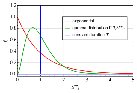
The $\gamma$ factor in equations (1b) and (1c) assumes that the time that a given Infectious becomes Removed is random, so one can only assert that the overall rate of transformation of Infectious to Recovered is proportional to the overall number of Infectious. In the absence of new infections, i.e. if $\beta=0$, the solution to equation (1b) is that the fraction of Infectious decreases exponentially in time: $I(t)=I(t_{1})\,\exp\left[-\gamma(t-t_{1})\right]$. This is the same equation as that of radioactive decay (which is experimentally verified). The time $t$ is unbounded. Therefore, instead of a popular conception that duration of infection is constant, it follows instead an exponential distribution in the SIR model. This explains why a 15-day fully-efficient lockdown is insufficient to eradicate a virus. This is illustrated in Figure 2, which shows the distribution of infectious times for 3 models: exponential (as in SIR), single-valued (as many people naïvely believe) and a gamma distribution that corresponds to the convolution of two identical exponential distributions. At 3 times the mean Infectious duration, the fraction of remaining Infectious is 5% in the exponential model and 0.6% in the gamma model. Quarantine times are set to ensure that nearly all Infectious recover, but one should remember that in models where the distribution of the infectious time is exponential or convolutions of exponentials, there is always a small fraction of Infectious that remain so at the end of the quarantine.

Insight is obtained by considering the basic reproduction number, which is defined as the ratio of the transmission to removal rates:

$$R_{0}={\beta\over\gamma}\ .$$ (2)

Equation (2) can also be re-written as $R_{0}$ being the ratio of the infectious period to the time between infectious contacts of an Infectious with Susceptible people. The differential equations can then be written

$$[left=\empheqlbrace\,]\dot{S} =-R_{0}\,S\,{I\over T_{\mathrm{I\to R}}}\ ,$$ (3a)

$$\dot{I} =\left(R_{0}\,S-1\right)\,{I\over T_{\mathrm{I\to R}}}\ ,$$ (3b)

$$\dot{R} ={I\over T_{\mathrm{I\to R}}}\ .$$ (3c)

The fraction of Infectious grows as long as $R_{0}>1/S$. At the beginning of the pandemic, $S\simeq 1$, and the criterion for growth is $R_{0}>1$. If the fraction of Susceptibles is appreciably decreased, the condition for continued growth of the pandemic is $R_{0}>1/S>1$.

Figure 3: Left: Evolution of daily cases, $-\dot{S}$, (blue) and deaths plus recovered, $\dot{R}$, (red) in the SIR model, for $R_{0}=4$ before lockdown and $R_{0}=0.5$ during lockdown, with $T_{\mathrm{I\to R}}=5\,\rm days$. Right: Observed evolution of daily cases for France for hospitalizations (blue) and deaths plus releases (red). In both panels, the lockdown is shown in the (shaded grey region). The decrease in observed cases and removed (deaths plus released) respectively occurred 14 and 25 days after the start of the lockdown, contrary to SIR prediction of immediate effects.

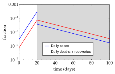
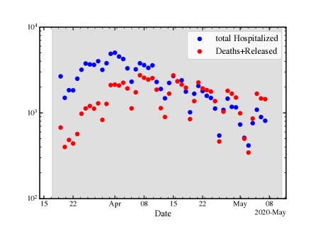
A numerical integration of the daily cases ($-\dot{S}$) and daily deaths and recoveries ($\dot{R}$) predicted from the SIR model in a context of a lockdown phase is illustrated in Figure 3. In the left panel, one sees that the SIR model predicts an immediate sharp decrease in the daily Removed (deaths and recoveries) with a discontinuous drop in new cases at the start of lockdown and a parallel but lower number of new cases relative to new deaths. The hospital data for all of France (right panel) indicates instead that both the new cases and daily Removed keep increasing after the start of the lockdown for roughly 14 and 25 days, respectively. The subsequent decreases are slower than in the SIR predictions. We thus begin our modeling with a SEIR model, extended to include hospital data.

2.2 SEIHCDRO model

Figure 4: Illustration of the SEIHCDRO model. The Infectious, Hospitalized and Critical phases are deemed Infectious, but only the Infectious phase people effectively infect the Susceptibles. Hospital data is available for the 4 phases in cyan-surrounded boxes. Also shown in the large red and green boxes are the Infectious and Immunized super-phases.

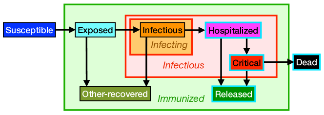
We extend the SEIR model (where E is for Exposed but not contagious) with the SEIHCDRO model, which includes the 7 following phases:

Susceptibles (S)

People who may catch the virus infection, without being immune to it.

Infectious (I)

People who are in an infectious stage, but not hospitalized

Hospitalized (H)

People who are treated for COVID-19 in hospitals, but are not in the critical care.

Critical (C)

People who are in a critical care at a hospital.

Dead (D)

People who died of COVID-19 at a hospital.

Released (R)

People who have been released from a hospital for COVID-19 treatment.

Other-Recovered (O)

People who have recovered from the virus, without having passed through a hospital.

The SEIHCDRO model, illustrated in Figure 4, includes branching fractions for transitions one phase to two possible others. Only a fraction of Exposed become Infectious (the remaining are similar to the Other-Recovered). Only a fraction of Infectious are Hospitalized, while the remaining eventually recover and join the Other-Recovered phase. Only a fraction of Hospitalized go to Critical care, while the remaining eventually are Released. Only a fraction of Critical people die, while the remaining are Released. The Other-Recovered are kept separate from the Released, because we only have data on the latter.

In the SEIHCDRO model, the infection of hospital workers by people in the Hospitalized and Critical phases is assumed to be negligible in comparison with the infection of the general population by the Infectious phase people. Indeed, Infectious people, who are often not aware of the contagiousness, meet many more Susceptibles than do Hospitalized or Critical phase people.

The equations of the SEIHCDRO model are

$$[left=\empheqlbrace\,]\dot{S} =-R_{0}\,S\,{I\over\overline{T}_{\rm I\to}}=-R_{0}\,S\,\left[{f_{\mathrm{I\to H}}\over T_{\mathrm{I\to H}}}+{(1-f_{\mathrm{I\to H}})\over T_{\mathrm{I\to O}}}\right]\,I\ ,$$ (4a)

$$\dot{E} =R_{0}\,S\,{I\over\overline{T}_{\rm I\to}}-f_{\mathrm{E\to I}}\,{E\over T_{\mathrm{E\to I}}}=R_{0}\,S\,\left[{f_{\mathrm{I\to H}}\over T_{\mathrm{I\to H}}}+{(1-f_{\mathrm{I\to H}})\over T_{\mathrm{I\to O}}}\right]\,I-f_{\mathrm{E\to I}}\,{E\over T_{\mathrm{E\to I}}}\ ,$$ (4b)

$$\dot{I} =f_{\mathrm{E\to I}}\,{E\over T_{\mathrm{E\to I}}}-{I\over\overline{T}_{\rm I\to}}=f_{\mathrm{E\to I}}\,{E\over T_{\mathrm{E\to I}}}-\left[{f_{\mathrm{I\to H}}\over T_{\mathrm{I\to H}}}+{(1-f_{\mathrm{I\to H}})\over T_{\mathrm{I\to O}}}\right]\,I\ ,$$ (4c)

$$\dot{H} ={\color[rgb]{0.7,0.0,0.0}f_{\mathrm{I\to H}}\,{I\over T_{\mathrm{I\to H}}}}-f_{\mathrm{H\to C}}\,{H\over T_{\mathrm{H\to C}}}-(1-f_{\mathrm{H\to C}})\,{H\over T_{\mathrm{H\to R}}}\ ,$$ (4d)

$$\dot{C} ={\color[rgb]{0.7,0.0,0.0}f_{\mathrm{H\to C}}\,{H\over T_{\mathrm{H\to C}}}}-f_{\mathrm{C\to D}}\,{C\over T_{\mathrm{C\to D}}}-(1-f_{\mathrm{C\to D}})\,{C\over T_{\mathrm{C\to R}}}\ ,$$ (4e)

$$\dot{D} ={\color[rgb]{0.7,0.0,0.0}f_{\mathrm{C\to D}}\,{C\over T_{\mathrm{C\to D}}}}\ ,$$ (4f)

$$\dot{R} ={\color[rgb]{0.7,0.0,0.0}(1-f_{\mathrm{H\to C}})\,{H\over T_{\mathrm{H\to R}}}}+{\color[rgb]{0.7,0.0,0.0}(1-f_{\mathrm{C\to D}})\,{C\over T_{\mathrm{C\to R}}}}\ ,$$ (4g)

$$\dot{O} =(1-f_{\mathrm{I\to H}})\,{I\over T_{\mathrm{I\to O}}}\ .$$ (4h)

In red are highlighted the terms contributing to the hospital data. Since $S+E+I+H+C+D+R+O=1$, one can omit equation (4h) and determine the Other-Recovered fraction, using $O=1-(S+E+I+H+C+D+R)$. The differential equations are written assuming that the timescales are all different even for evolution of one phase into two possible future phases. One notes that the independent parameters are the $R_{0}$ factor as well as 7 ratios of timescales to branching fractions, i.e. $T_{\mathrm{E\to I}}/f_{\mathrm{E\to I}}$, $T_{\mathrm{I\to H}}/f_{\mathrm{I\to H}}$, $T_{\mathrm{H\to C}}/f_{\mathrm{H\to C}}$, $T_{\mathrm{C\to D}}/f_{\mathrm{C\to D}}$, $T_{\mathrm{H\to R}}/(1-f_{\mathrm{H\to C}})$, $T_{\mathrm{C\to R}}/(1-f_{\mathrm{C\to D}})$, and $T_{\mathrm{I\to O}}/(1-f_{\mathrm{I\to H}})$. Thus, the timescales and conjugate branching fractions are degenerate, but a constraint on the ratio provides an upper limit to the timescale.

2.3 The SEAFHCDRO model

Figure 5: Illustration of the SEAFHCDRO model, with same comments as in Fig. 4. Only the Asymptomatics effectively infect the Susceptibles.

The SEIFHCDRO model can be generalized by splitting the Infectious compartment into one where people effectively contaminate the Susceptibles, and another where people are too ill to go outside and contaminate Susceptibles. These new compartments are called the Asymptomatic and Feverish phases (see Fig. 5).

The equations of the SEAFHCDRO model are

$$[left=\empheqlbrace\,]\dot{S} =-R_{0}\,S\,{A\over\overline{T}_{\rm A\to}}=-R_{0}\,S\,\left[{f_{\mathrm{A\to F}}\over T_{\mathrm{A\to F}}}+{(1-f_{\mathrm{A\to F}})\over T_{\mathrm{A\to O}}}\right]\,A\ ,$$ (5a)

$$\dot{E} =R_{0}\,S\,{A\over\overline{T}_{\rm A\to}}-f_{\mathrm{E\to A}}\,{E\over T_{\mathrm{E\to A}}}=R_{0}\,S\,\left[{f_{\mathrm{A\to F}}\over T_{\mathrm{A\to F}}}+{(1-f_{\mathrm{A\to F}})\over T_{\mathrm{A\to O}}}\right]\,A-f_{\mathrm{E\to A}}\,{E\over T_{\mathrm{E\to A}}}\ ,$$ (5b)

$$\dot{A} =f_{\mathrm{E\to A}}\,{E\over T_{\mathrm{E\to A}}}-{A\over\overline{T}_{\rm A\to}}=f_{\mathrm{E\to A}}\,{E\over T_{\mathrm{E\to A}}}-\left[{f_{\mathrm{A\to F}}\over T_{\mathrm{A\to F}}}+{(1-f_{\mathrm{A\to F}})\over T_{\mathrm{A\to O}}}\right]\,A\ ,$$ (5c)

$$\dot{F} =f_{\mathrm{A\to F}}\,{A\over T_{\mathrm{A\to F}}}-f_{\mathrm{F\to H}}\,{F\over T_{\mathrm{F\to H}}}-(1-f_{\mathrm{F\to H}}){F\over T_{\mathrm{F\to O}}}\ \ ,$$ (5d)

$$\dot{H} ={\color[rgb]{0.7,0.0,0.0}f_{\mathrm{F\to H}}\,{F\over T_{\mathrm{F\to H}}}}-f_{\mathrm{H\to C}}\,{H\over T_{\mathrm{H\to C}}}-(1-f_{\mathrm{H\to C}})\,{H\over T_{\mathrm{H\to R}}}\ ,$$ (5e)

$$\dot{C} ={\color[rgb]{0.7,0.0,0.0}f_{\mathrm{H\to C}}\,{H\over T_{\mathrm{H\to C}}}}-f_{\mathrm{C\to D}}\,{C\over T_{\mathrm{C\to D}}}-(1-f_{\mathrm{C\to D}})\,{C\over T_{\mathrm{C\to R}}}\ ,$$ (5f)

$$\dot{D} ={\color[rgb]{0.7,0.0,0.0}f_{\mathrm{C\to D}}\,{C\over T_{\mathrm{C\to D}}}}\ ,$$ (5g)

$$\dot{R} ={\color[rgb]{0.7,0.0,0.0}(1-f_{\mathrm{H\to C}})\,{H\over T_{\mathrm{H\to R}}}}+{\color[rgb]{0.7,0.0,0.0}(1-f_{\mathrm{C\to D}})\,{C\over T_{\mathrm{C\to R}}}}\ ,$$ (5h)

$$\dot{O} =(1-f_{\mathrm{A\to F}})\,{I\over T_{\mathrm{A\to O}}}+(1-f_{\mathrm{F\to H}}){F\over T_{\mathrm{F\to O}}}\ .$$ (5i)

2.4 The SEAFHDRO model

Figure 6: Illustration of the SEAFHDRO model, with same comments as Fig. 5

We shall see below that neither the SEIFHCDRO nor the SEAFHCDRO models are able to fit the evolution of the Critical population. Our final SEAFHDRO model (Fig. 6) therefore eliminates the Critical phase, by merging it with the Hospitalized phase. Its equations are

$$[left=\empheqlbrace\,]\dot{S} =-R_{0}\,S\,{A\over\overline{T}_{\rm A\to}}=-R_{0}\,S\,\left[{f_{\mathrm{A\to F}}\over T_{\mathrm{A\to F}}}+{(1-f_{\mathrm{A\to F}})\over T_{\mathrm{A\to O}}}\right]\,A\ ,$$ (6a)

$$\dot{E} =R_{0}\,S\,{A\over\overline{T}_{\rm A\to}}-f_{\mathrm{E\to A}}\,{E\over T_{\mathrm{E\to A}}}=R_{0}\,S\,\left[{f_{\mathrm{A\to F}}\over T_{\mathrm{A\to F}}}+{(1-f_{\mathrm{A\to F}})\over T_{\mathrm{A\to O}}}\right]\,A-f_{\mathrm{E\to A}}\,{E\over T_{\mathrm{E\to A}}}\ ,$$ (6b)

$$\dot{A} =f_{\mathrm{E\to A}}\,{E\over T_{\mathrm{E\to A}}}-{A\over\overline{T}_{\rm A\to}}=f_{\mathrm{E\to A}}\,{E\over T_{\mathrm{E\to A}}}-\left[{f_{\mathrm{A\to F}}\over T_{\mathrm{A\to F}}}+{(1-f_{\mathrm{A\to F}})\over T_{\mathrm{A\to O}}}\right]\,A\ ,$$ (6c)

$$\dot{F} =f_{\mathrm{A\to F}}\,{A\over T_{\mathrm{A\to F}}}-f_{\mathrm{F\to H}}\,{F\over T_{\mathrm{F\to H}}}-(1-f_{\mathrm{F\to H}}){F\over T_{\mathrm{F\to O}}}\ \ ,$$ (6d)

$$\dot{H} ={\color[rgb]{0.7,0.0,0.0}f_{\mathrm{F\to H}}\,{F\over T_{\mathrm{F\to H}}}}-f_{\mathrm{H\to D}}\,{H\over T_{\mathrm{H\to D}}}-(1-f_{\mathrm{H\to D}})\,{H\over T_{\mathrm{H\to R}}}\ ,$$ (6e)

$$\dot{D} ={\color[rgb]{0.7,0.0,0.0}f_{\mathrm{H\to D}}\,{H\over T_{\mathrm{H\to D}}}}\ ,$$ (6f)

$$\dot{R} ={\color[rgb]{0.7,0.0,0.0}(1-f_{\mathrm{H\to D}})\,{H\over T_{\mathrm{H\to R}}}}\ ,$$ (6g)

$$\dot{O} =(1-f_{\mathrm{A\to F}})\,{I\over T_{\mathrm{A\to O}}}+(1-f_{\mathrm{F\to H}}){F\over T_{\mathrm{F\to O}}}\ .$$ (6h)

As in the SIR model, the SEIHCDRO, SEAFHCDRO, and SEAFHDRO models all assume exponential probability distribution functions (pdfs) for the durations of the phases (besides S). But while the SIR model involves a single exponential pdf for the duration of the Infectious phase, in our more complex models, the infectious phases are split into several, each with an exponential pdf of duration, which effectively creates a different pdf for the duration of the entire infectious phase, i.e. the combination of (Infectious or Asymptomatic and Feverish), Hospitalized (and Critical) phases. Thus the pdf of the entire set of infectious phases is no longer exponential, but the convolution of different exponentials, which amounts to gamma or Erlang distributions, which both reach their maximum at a positive value of the duration.

2.5 Assumptions and caveats

The assumptions of the models presented above can be summarized as follows.

1. The probability distribution functions of the durations for the transition from one phase to the next are all assumed to be exponential, but with mean durations that depend on the particular transition.

2. Only fractions of the population advance to the next phase, hence the branching fractions $f_{\rm A\to B}$, which all lie between zero and unity, and are assumed different.

3. The free parameters are the $R_{0}$ factors (before and during lockdown), the normalization of the first phase of Infectious (i.e. Asymptomatic in the latter two models), and 7 (SEIFHCDRO and SEAFHDRO) or 9 (SEAHCDRO) ratios of timescales to branching fractions.

4. These free parameters are assumed to be fixed in time: i.e. the ratios of timescales to branching fractions are assumed fixed in time, and the $R_{0}$ factor is assumed to vary as a step function at the start of the lockdown.

5. The Feverish, Hospitalized, and Critical people are assumed to infect few others. The Feverish stay at home. The Hospitalized and Critical are assumed to infect a negligible number of Hospital staff. While this was not the case in the early phases of the pandemic in each country, where hospital staff were often infected by patients, my model assumes that by 1 March 2020 when the model starts, and especially starting on 18 March 2020, where the hospital data begins, the staff (doctors, nurses, and attendants) in French hospitals were sufficiently protected with face masks and with frequent hand washing and disinfection of their hands.

6. People who recover, whether out or in the hospital, are assumed to immediately lose their infectiousness. A possible continual of infectiousness is possible, at least in some of the recovered people. The guidelines from the American Centers for Disease Control and Prevention (CDC) recommend 3 days of isolation after recovery (Centers for Disease Control and Prevention, 2020). The modeling of a possible continuation of contagiousness in recovered people is straightforward (and has been performed by this author), but is beyond the scope of the present work.

3 Data

I used the daily COVID-19 hospital movements related to COVID-19 provided by Santé publique France at https://www.data.gouv.fr/fr/datasets/r/6fadff46-9efd-4c53-942a-54aca783c30c. This data lists the hospital arrivals $\dot{\cal H}$, the arrivals in critical care (reanimation) $\dot{\cal C}$, the deaths $\dot{\cal D}$, and the releases $\dot{\cal R}$. These values are given for the 96 French départements, plus 5 overseas ones. I only considered the 96 départements, assuming that the population was genetically homogeneous, leading to unique values of the mean durations of the phases and of the branching ratios. I either considered the 96 départements together as a single entity, called ‘single-zone France’, as well as 15 regions, corresponding to the 13 French régions, but splitting région Île-de-France around the capital into three units: Paris, Paris-Petite-Ceinture (surrounding 3 districts: Hauts de Seine [92], Seine-Saint-Denis [93], and Val de Marne [94]), and Paris-Grande-Ceinture (outer districts: Seine-et-Marne [77], Yvelines [78], Essonne [91], val d’Oise [95]).

The hospital data begins on 19 March 2020, and I used the values up to 3 May 2020, for a total of 46 days of data.

I assumed that by number of hospital arrivals $\dot{\cal H}$, the hospitals are including the number of arrivals into critical care. But there were a few (1%) cases where the hospital arrivals on a given date is smaller than the arrivals in critical care. In this case, I simply assumed that the new hospitalizations do not include the entries into critical care.

4 Analysis

4.1 Initial conditions

At the origin of time, 1 March 2020, I set all phases $X=0$, except the first Infectious phase ($I$ or $A$) which is given a small value (whose logarithm is a free parameter) and the Susceptibles which initially satisfy $S=1-I$ or $S=1-A$, depending on the model. The date of 1 March 2020 was not chosen at random, but corresponds to 3 days after the start of the exponential growth in France. Some regions only saw exponential growth several days later, so 1 March was chosen as a compromise between the early regions (around Mulhouse in the Grand-Est) and the late regions (west of France).

4.2 Free parameters

As mentioned above, the free parameters are two $R_{0}$ factors (before and after lockdown), the normalization of the earliest Infectious phase, and 7 or 9 ratios of timescales to branching fractions. I have analyzed France as a single zone in this manner, and the computations are rapid. But one can obtain a tighter constraint on the ratios of timescales to branching fractions by joint modeling several zones of France, all assumed to be genetically homogeneous, i.e. with the same time-over-fraction ratios, but allowing for different $R_{0}$ factors before and during lockdown, as well as different normalizations. The total number of free parameters were then $N_{\rm time-over-fraction}+3\,N_{\rm zones}$, i.e. up to 54 free parameters (for 15 regions in the SEAFHCDRO model).

4.3 Likelihood

Given the hospital data

$$\dot{\cal X}_{i}\equiv\left\{\dot{\cal H},[\dot{\cal C},]\dot{\cal D},\dot{\cal R}\right\}\ ,$$ (7)

the likelihood of my models is written

$$-\ln{\cal L}=-\sum_{i=1}^{N_{\rm zones}}\,\sum_{j=1}^{N_{\rm times}}\,\sum_{k=1}^{N_{\rm phases}}\ln{\rm Poisson}\left(\dot{\cal X}_{k}(t_{j},i)\,|\,{\rm Population}_{i}\,f_{i,k}\left(t_{j},\right)\right)\ ,$$ (8)

where $f_{i,k}\left(t_{j}\right)$ represents the predicted number of daily arrivals into phase ${\cal X}_{k}$ in zone $i$ on day $j$.

4.4 MCMC analysis

Table 1: Priors on free parameters

Parameter	minimum	maximum
fractions	0	1
log (durations/days)	0	2
$R_{0}$ before lockdown ($R_{0}^{\rm Ini})$	1	6
$R_{0}$ after lockdown ($R_{0}^{\rm Conf})$ in units of $R_{0}^{\rm Ini}$	0	1
log fraction of Asymptomatics on 1 March 2020	–8	–3

Notes: The logarithms are in base 10.

Marginal distributions of the free parameters and of the evolution of the pandemic in France were obtained through a Markov-Chain Monte Carlo (MCMC) model. The code was written in Python 3, and the marginal distributions of the free parameters were estimated from the posteriors using the emcee package Goodman and Weare (2010). The MCMC procedure involved a minimum of number of chains (or “walkers”) equal to twice the number of free parameters, with a minimum of 64 (for single-zone models), and up to 119 for 15-region models, and up to near 600 for 96-department runs. The chains (walkers) are advanced using the stretch move algorithm (Goodman and Weare, 2010). These chains were initialized with uniform sampling over the allowed range of parameters shown in Table 1. The chains were run for 200 000 steps (single zone) or 50 000 steps (15 regions), thus involving a total of several million evaluations of the set of differential equations. I assumed 80% burnin factor, thus only considering the last 20% of each chain for the analysis. The figures showing curves, use medians for the curves with shaded regions for 16-84% and 5-95% confidence levels.

5 Results

5.1 Goodness-of-fits

Figure 7: Goodness-of-fit results for single-zone France. The symbols show the daily hospital data (arrivals in magenta, arrivals in critical care in red, deaths in black, released in green), with Poisson error bars. The curves are the median predictions from the SEIHCDRO (left) and SEAFHCDRO (right) models (both fitting to data up to 3 May), while the narrow and wider shaded areas respectively show the extent of 16th-84th and 5th-95th percent confidence levels.

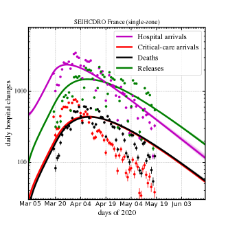
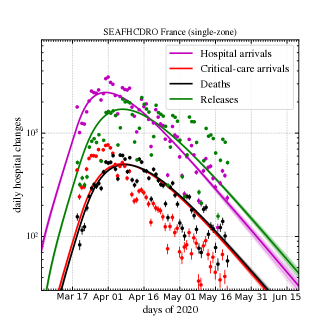
Figure 7 shows the goodness of fit of single-zone France for the SEIHCDRO and SEAFHCDRO models. The daily hospitalizations (magenta), deaths (black) and releases (green) are well fit by the models, especially for the SEAFHCDRO model (right), while the SEIHCDRO model predicts too early a peak in daily hospital arrivals. However, the daily arrivals in critical care are poorly fit by the models, which cannot reproduce the early narrow peak in the last days of March, followed by the rapid decrease. One also notices that the mean values of the post-burnin marginal distributions of $R_{0}$ lead to very high values before the lockdown: $R_{0}=6$ (the allowed upper limit) for model SEIRHCDRO and $R_{0}=4.24\pm 0.1$ for model SEAFHCDRO. At the same time, the values during lockdown are found to be very small: $R_{0}=0.18\pm 0.02$ and $0.01\pm 0.02$ for SEIRHCDRO and SEAFHCDRO, respectively.

Figure 8: Same as Figure 7, again for the SEIHCDRO (left) and SEAFHCDRO (right) models, but for Paris from the 15-region analysis.

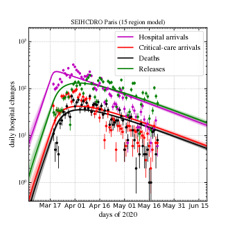
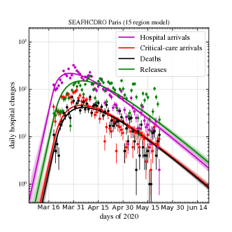
Figure 8 shows the same trends for the city of Paris, when running models SEIHCDRO (left) and SEAFHCDRO (right) with the 15 regions. One notices the same poorly-fit data for the arrivals in critical care as for all of France. Since France contributes roughly 10% of France in terms of critical care arrivals, this suggests that the dichotomy between model predictions and data for critical care arrivals is general throughout France (not shown in the figures). This dichotomy with the models cannot be caused by saturated critical care, because it occurs in all regions, while only a few suffered from critical care unit saturation. Interestingly, a hospital official mentioned that France has learned how to better treat COVID-19 patients and has been sending progressively smaller fractions to critical care.

With joint modeling of 15 regions, the $R_{0}$ values before and during lockdown are respectively lower and higher than for single-Zone France, suggesting that the lockdown is less effective than for single-zone France, where $R_{0}$ is reduced by a factor of at least 30. For Paris, the $R_{0}$ factors before lockdown are $R_{0}=2.65\pm 0.20$ for SEIHCDRO and $R_{0}=3.5\pm 0.2$ for SEAFHCDRO. At the same time, the lockdown values of $R_{0}$ is not as low for Paris than for the single-zone France model: $R_{0}=0.91\pm 0.05$ and $R_{0}=0.65\pm 0.20$ for models SEIHCDRO and SEAFHCDRO, respectively.

Figure 9: Goodness-of-fit for the SEAFHDRO model (i.e. with Critical phase merged into Hospitalized) for single-zone France (left) and for Paris in the 15-region run (right), both fitting data up to 10 May.

The comparison of the quality of the fits between the SEIHCDRO and SEAFHCDRO models is performed using BIC Bayesian evidence

$${\rm BIC}=-2\,\ln{\cal L}_{\rm MLE}+N_{\rm parameters}\,\ln N_{\rm data}\ ,$$ (9)

where ${\cal L}_{\rm MLE}$ is the maximum likelihood. BIC effectively compares the log-likelihoods, but penalizes extra free parameters, especially in large data sets (as is the case here). Such a test can only be done on the same amount of data, which is the case for these two models. In all cases studied, including single-zone France, the SEAFHCDRO has lower BIC than SEIRHCDRO, by typically over 1000, whereas a difference of 6 is deemed strong evidence.

The better fits of the SEAFHCDRO model led me to drop the SEIHCDRO model. Moreover, the general dichotomy between the predicted and observed arrivals to critical care led me to also consider the SEAFHDRO model, which folds the Critical phase into the Hospitalized phase.

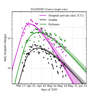
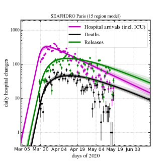
Figure 9 shows the goodness-of-fits of the SEAFHDRO model for the single-Zone France as well as for Paris in the 15-region run. The fits remain good for the daily Hospital arrivals (magenta) and the hospital Releases (green), but now fail somewhat to describe the decrease in the daily deaths (black). Moreover, even if one cannot use the BIC Bayesian evidence, because the number of data points is not the same, we note that a naïve correction of the $-\cal{L}_{\rm MLE}$ by 4/3 for SEAFHDRO leads to a value 18 above that of SEAFHCDRO,

All models used here predict that the daily Deaths should evolve in parallel to the daily Releases, with a possible time lag, whereas the data indicates that the Deaths fall more rapidly than the Releases (see Figs. 7, 8, and 9).

5.2 Timescales and branching fractions

Figure 10: Marginal distributions of timescales over branching fractions for the single-zone France (top) and 15-region (bottom) runs for models SEAFHCDRO (left) and SEAFHDRO (right). The boxes indicate the geometric mean timescales over branching fractions.

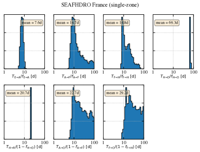
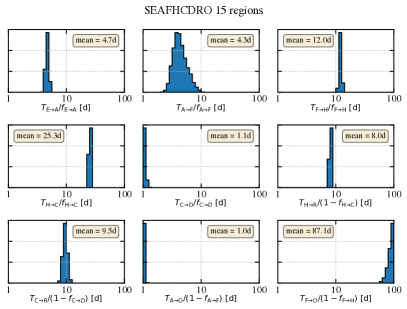
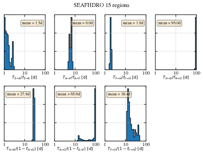
Figure 10 displays the marginal distributions of ratios of timescales to branching fractions for the SEAFHCDRO (left) and SEAFHDRO (right) models (with two fewer ratios), for single-zone France (top) and 15 regions (bottom). One first notes that the joint fit of 15 regions allows much narrower constraints on the ratios than the single-zone France fit. This is most striking for ratios $T_{\mathrm{F\to H}}/f_{\mathrm{F\to H}}$ and $T_{\mathrm{A\to O}}/(1-f_{\mathrm{A\to F}})$, whose marginal distribution go from very wide (single-zone France) to very narrow (15 regions).

Several results can be inferred from these marginal distributions of ratios of timescales to branching fractions. In particular, since the timescale is necessarily less than the ratio, Figure 10 provides upper limits on timescales. The top left panel of the 15-region models (lower sets of panels) indicates that the incubation time, $T_{\mathrm{E\to A}}$, is at most a few days (95% confidence upper limits of 5.1 and 2.7 days according to models SEAFHCDRO and SEAFHDRO, respectively). The time for strong symptoms to appear, $T_{\mathrm{A\to F}}$, is shorter than 7.1 days (95% c.l.). The time to recover from the Feverish phase, $T_{\mathrm{F\to O}}$ is large, or else the fraction of Feverish that end up Hospitalized is near unity, which seems less likely.

Several marked differences appear between the two models: The ratio $T_{\mathrm{F\to H}}/f_{\mathrm{F\to H}}$ is less than 2 days for SEAFHDRO in contrast to less than 13 days for SEAFHCDRO (both at 95% c.l.). And the time for Asymptomatics to recover, $T_{\mathrm{A\to O}}$, is less than 1.1 days (95% c.l.) for SEAFHCDRO, but possibly as long as 100 days for SEAFHDRO. Finally, while the time from Critical to Death is shorter than 1.2 days (95% c.l.) in the SEAFHCDRO model, the ratio $T_{\mathrm{H\to D}}/f_{\mathrm{H\to D}}$ is peaked at 100 days (the allowed maximum, see Table 1). While these two measures are not directly comparable, this may mean that only a small fraction of hospitalized eventually die in the hospital.

5.3 The effects of lockdown on basic reproduction factors

Figure 11: Marginal distributions of basic reproduction factors of 15 French regions before (left) and during (right, with shifted scale) lockdown for models SEAFHCDRO (top) and SEAFHDRO (bottom). The $x$-axis limits reflect the range of priors, except for the bottom right panel, where the free parameter was $R_{0}^{\rm Conf}/R_{0}^{\rm Ini}$, whose prior was flat between 0 and 1.

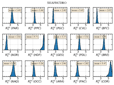
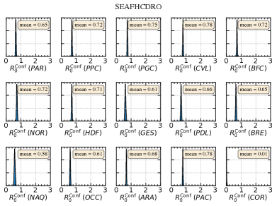
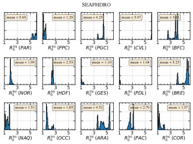
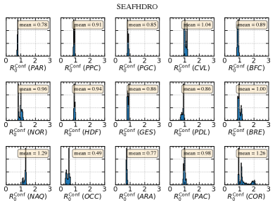
Figure 11 shows the marginal distributions of $R_{0}$ for the 15 regions of France before (left) and during (right) lockdown for the SEAFHCDRO (top) and SEAFHDRO (bottom) models. Table 2 provides means and 90% confidence limits for each region and also provides mean values weighted by the populations of the regions. Of course, the $R_{0}$ factors during the lockdown were well below the values before the lockdown. This means that the lockdown had a noticeable effect on the reproduction factor.

Table 2: $R_{0}$ values by region

Abb.	Name	$R_{0}$ (before lockdown)			$R_{0}$ (during lockdown)
		SEAFHCDRO	SEAFHDRO		SEAFHCDRO	SEAFHDRO
PAR	Paris	3.49 [3.17:3.85]	5.69  [5.27:5.99]		0.65 [0.62:0.69]	0.78 [0.74:0.81]
PPC	Paris-Petite-Ceinture	3.46 [3.31:3.65]	1.29  [1.10:1.50]		0.72 [0.69:0.75]	0.91 [0.86:0.96]
PGC	Paris-Grande-Ceinture	2.40 [2.23:2.56]	4.25  [3.57:4.53]		0.75 [0.72:0.78]	0.85 [0.81:0.90]
CVL	Centre - Val de Loire	5.65 [5.49:5.82]	5.97  [5.91:6.00]		0.78 [0.75:0.82]	1.04 [0.95:1.17]
BFC	Bourgogne-Franche-Comté	2.02 [1.84:2.21]	3.61  [2.57:4.09]		0.72 [0.69:0.75]	0.89 [0.84:0.95]
NOR	Normandie	2.02 [1.77:2.24]	1.99  [1.86:2.21]		0.72 [0.67:0.77]	0.96 [0.82:1.12]
HDF	Hauts de France	5.71 [5.23:5.96]	2.53  [2.37:2.67]		0.71 [0.68:0.75]	0.94 [0.89:0.99]
GES	Grand Est	3.17 [2.77:3.53]	1.10  [1.00:1.39]		0.61 [0.56:0.67]	0.86 [0.80:0.91]
PDL	Pays de Loire	3.32 [3.07:3.56]	1.04  [1.00:1.16]		0.66 [0.62:0.70]	0.86 [0.72:0.93]
BRE	Bretagne	3.79 [3.49:4.03]	5.23  [4.02:5.75]		0.65 [0.60:0.69]	1.00 [0.89:1.17]
NAQ	Nouvelle Aquitaine	3.79 [3.28:4.20]	1.51  [1.12:1.82]		0.58 [0.52:0.64]	1.29 [1.12:1.36]
OCC	Occitanie	3.26 [3.01:3.54]	1.85  [1.56:2.66]		0.61 [0.57:0.64]	0.49 [0.33:0.63]
ARA	Auvergne-Rhône-Alpes	2.96 [2.68:3.31]	4.52  [3.52:5.44]		0.68 [0.65:0.71]	0.77 [0.74:0.81]
PAC	Provence:Côte d’Azur	2.82 [2.47:3.14]	2.79  [2.35:3.19]		0.78 [0.75:0.81]	0.98 [0.90:1.08]
COR	Corse	5.47 [4.87:5.88]	1.37  [1.06:2.02]		0.01 [0.00:0.04]	1.26 [0.93:2.01]
	Weighted Average	3.43 [3.31:3.51]	2.84  [2.65:3.10]		0.65 [0.61:0.69]	0.88 [0.86:0.93]

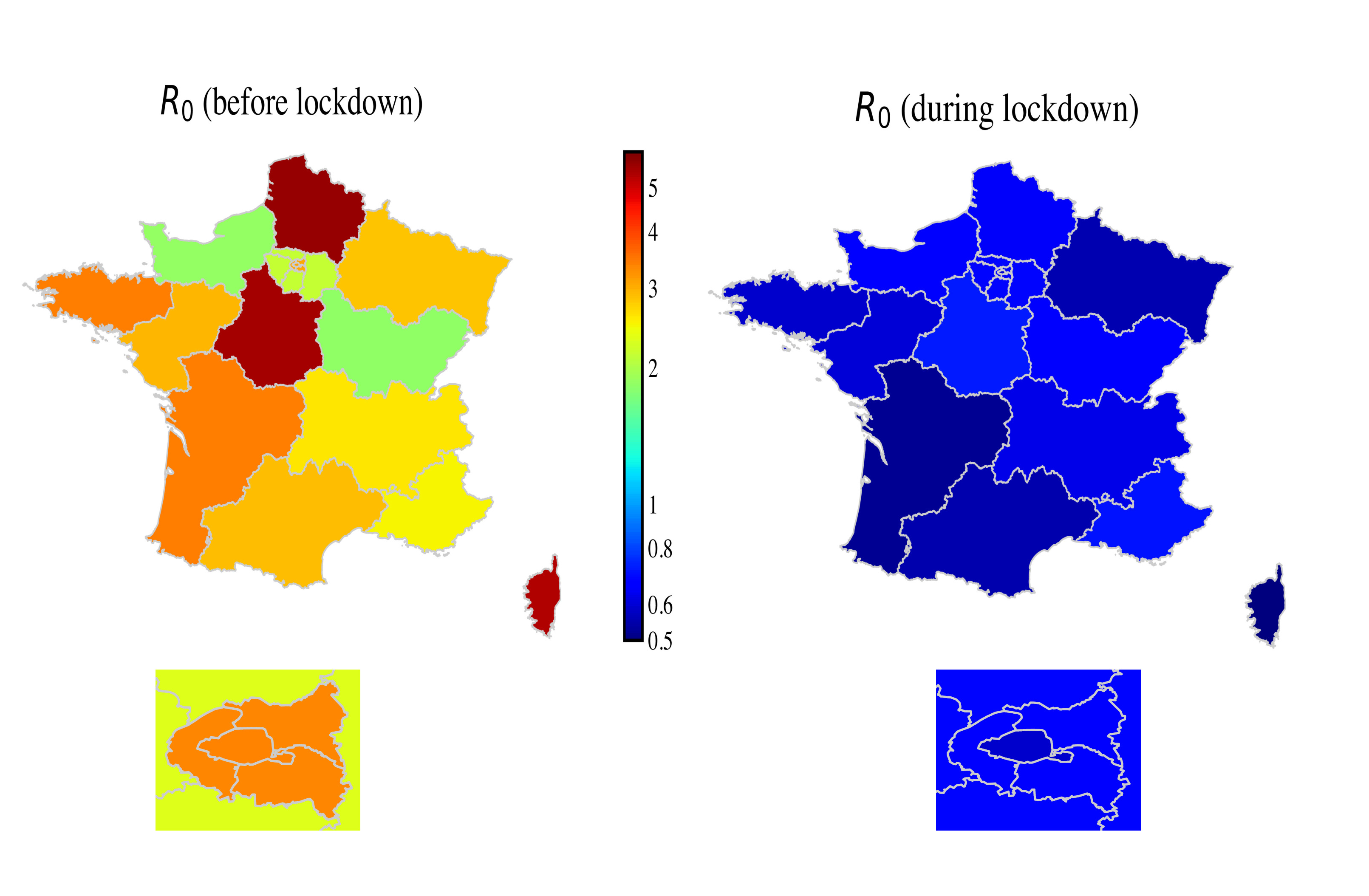
The $R_{0}$ values are listed in Table 2. The population-weighted mean values are given at the bottom row of the Table. The mean $R_{0}$ values before lockdown are 3.43 [3.31 to 3.51] for SEAFHCDRO and 2.84 [2.65 to 3.10] for SEAFHDRO (showing 90% confidence intervals in brackets). The corresponding values during lockdown are 0.65 [0.61 to 0.69] for SEAFHCDRO and 0.88 [0.86 to 0.93] for SEAFHDRO. Therefore the lockdown had a strong effect as it reduced $R_{0}$ by factor of over 5 (SEAFHCDRO) or over 3 (SEAFHDRO). This can graphically seen in Figure 12, which confirms the overall success of the lockdown.

The city of Paris displays a high $R_{0}$ before the lockdown, which is expected given its very large population density. Surprisingly, region Centre Val de Loire displays even higher $R_{0}$ for both models. Region Grand Est, where the pandemic hit early and hard, shows a low pre-lockdown $R_{0}$, probably because its inhabitants self-confined well before the lockdown. This is also true for Paris, whose inhabitants knew they were at great risk because of the high population density, which may explain why its pre-lockdown $R_{0}$ is not even higher.

Figure 12: Maps of basic reproduction factors in France (top) and Paris area (bottom) before (left) and during (right) lockdown for the SEAFHCDRO model.

However, there are important differences in the marginal distributions of $R_{0}$ between the 2 models, as displayed in Figure 11. Some regions are among the lowest in pre-lockdown $R_{0}$ with SEAFHDRO, while they are among the highest with SEAFHCDRO, e.g. Paris-Petite-Ceinture and Hauts de France. With SEAFHDRO, Pays de Loire and Centre Val de Loire are at respectively the lower and upper limits of our pre-lockdown prior ($R_{0}=1$, see Table 1), while they show normal values of $R_{0}$ with SEAFHCDRO. While the $R_{0}$ values during the lockdown are all below unity for SEAFHCDRO, a few regions with the SEAFHDRO model show lockdown $R_{0}$ values above unity: Centre val de Loire, Bretagne, and especially Nouvelle Aquitaine and Corse.

These issues suggests that SEAFHCDRO is a better model compared to its SEAFHDRO counterpart. In what follows, I will therefore concentrate on the SEAFHCDRO model.

5.4 Past and future evolution

5.4.1 Evolution with no lifting of lockdown

The evolution of the 9 SEAFHCDRO phases is shown in Figure 13. All four panels show interesting features: the Exposed population has a sharp turn from exponential growth before lockdown to exponential decrease once the lockdown has started. The subsequent phases show increasingly more moderate and delayed reactions to the lockdown. Another interesting feature is that, SEAFHCDRO run on 15 regions allows fairly precise measures of the different phases, including the early ones, which are naturally less well constrained by the hospital data. Despite having one-tenth of the hospital data of the country, the city of Paris displays impressively precise estimates on the 9 phases. This is true of all regions.

The bottom panels of Figure 13 show the same, but for single-zone runs of France (left) and Paris (right). Here, the Hospitalized, Critical, Dead and Released phases still show low uncertainties, thanks to the available hospital data. However, the uncertainties on the pre-Hospitalized phases (Exposed, Asymptomatic, and Feverish) are now high. In particular, while the Feverish (orange) curves are thin in the 15-region (top) panels, they are very thick for the single-zone (bottom) ones. This difference is related to the apparent degeneracy between terms $F$ and $T_{\mathrm{F\to H}}/f_{\mathrm{F\to H}}$ in equation 5e. Without extra information, the degeneracy causes a strong uncertainty on the Feverish population fraction, $F$. But with the additional knowledge of the time-to-fraction ratios, such as $T_{\mathrm{F\to H}}/f_{\mathrm{F\to H}}$ given by multi-zone runs, the degeneracy is lifted and the uncertainty on $F$ is small. This confirms the use of computer-expensive multiple-zone runs to better constrain the time-to-branching-fraction ratios.

Figure 13: Top: Evolution of the 9 SEAFHCDRO phases in the 15-region model for France (weighted average, left) and Paris (right). The curves are the mean post-burnin values, while the shaded and light-shaded areas represent 16-85% and 5-95% confidence limits. Bottom: Same for single-zone France (left) and single-zone Paris (right).

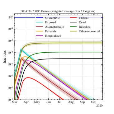
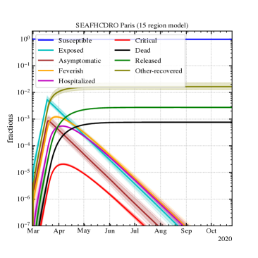
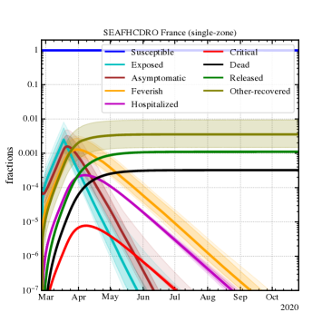
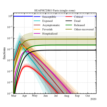
The top panels of Figure 13 indicate that if the lockdown were not partially lifted on 11 May 2020, the number of Dead would only very mildly rise, to fractions of 0.03% for France as a whole (i.e. 20 thousand deaths) and 0.08% for Paris (1800 deaths). In fact on 11 May 2020, France had suffered 26 000 deaths, and the underestimate from our model are within the statistical uncertainties. The huge majority of the population remains Susceptible.

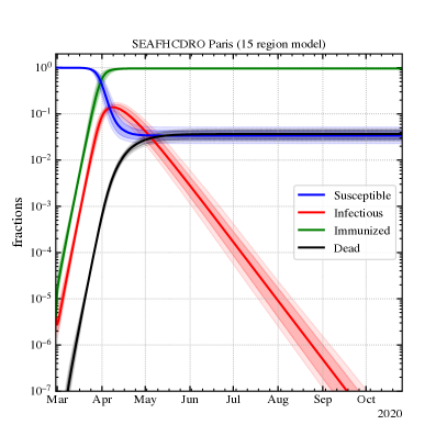
Figure 15 shows the evolution of the 4 super-phases: Susceptible, Infectious, Immunized, and Dead (see Fig. 5). The total fraction of Infectious (i.e. Asymptomatic, Feverish, Hospitalized, and Critical), which reached a maximum of several tenths of one percent in the 2nd half of March, has decreased by a factor 10 (single-zone France) or 6 (Paris in 15-region analysis) by 11 May 2020. Thus, on 11 May 2020, the total fraction of Infectious should be a few per ten thousand.

Figure 14: Maps of fraction of Immunized in France on 11 May 2020, with SEAFHCDRO model (median of marginal distributions).

The fraction of Immunized (all but Susceptibles and Dead) is less than 1% for all of France (weighted average over the 15 regions), and 3% for Paris, both at the 95% confidence level. A map of France of the fraction of Immunized on 11 May 2020 is displayed in Figure 14. One notices that Paris and the Grand Est region have the highest immunized fractions up to 2%, followed by the inner ring around Paris. The lowest fractions of Immunized all lie in the West of France, where the fraction of Immunized is 10 times lower than in Paris.

These low fractions of Immunized means that France has not reached herd immunity and is therefore sensitive to a second wave of the pandemic. The fraction of Immunized is lower in the SEAFHDRO model (not shown in Fig. 15), at less than 0.3% on May 11, rising to over 1% in August, again insufficient for herd immunity.

Figure 15: Simplification of the 9 phases into 4 super-phases, for the 15-region model.

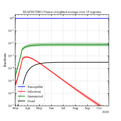
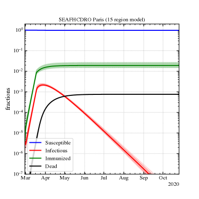
Figure 15 allows one to estimate the Infectious Fatality Rate, IFR = Deaths/Immunized. After early July 2020, the IFR stabilizes to values of 4% (with a factor 30% relative uncertainty) for both France and Paris with the 15-region analysis. The values measured at 11 May 2020 are only slightly lower. The SEAFHDRO model (not shown in Fig. 15) leads to a much higher (but less plausible to this author) IFR of 12$\pm$2% averaged over France.

These values are quite high, but France also currently has a very high Case-Fatality-rate, which has reached a plateau of 20% since early May 2020.

5.4.2 How many deaths, had there been no lockdown nor social distancing?

Figure 16: Prediction of evolution had there been: no lockdown on 17 March 2020 (left) or a lockdown 10 days earlier (7 March 2020, right), both with the SEAFHCDRO model run with 15 regions, for France (weighted average).

The modeling of the French hospital data presented here allows to estimate the number of Dead in the absence of lockdown and of social distancing. It suffices to adopt the marginal distributions of the ratios of timescales to branching fractions, as well as the marginal distributions of pre-lockdown $R_{0}$ factors for each region.

The left panel of Figure 16 shows the evolution of the 4 super-phases in the absence of any lockdown or social distancing with the SEAFHCDRO model. The fraction of Dead would would have surpassed 1% by mid-April. By early June 2020, the fraction of Dead would have reached its plateau at 3.5$\pm$1% (The uncertainties are 90% confidence) for France, and 4$\pm$1.5% for Paris. In other words, France would have suffered over 2 million deaths without a lockdown! Using instead the SEAFHDRO model (not shown in Fig. 16), the fraction of Dead would have been 3 times higher resulting in over 7 million deaths. These are in fact lower limits, because the hospitals would been completely saturated, leading to even more casualties.

5.4.3 How many deaths would have been avoided with an earlier lockdown?

One can similarly estimate the amount of deaths in France had the lockdown been enforced 10 days earlier. Indeed, By 5 March 2020, France had suffered a full week of daily doubling of cases and deaths, and the situation in the Grand Est, in particular the city of Mulhouse was becoming out of control. Assuming (probably optimistically) that it would take one day of decision-making and one day for preparing the lockdown, the earliest possible starting date for the national lockdown in France would have been on 7 March 2020. The right panel of Figure 16 shows the evolution of the super-phases with this earlier lockdown. The fraction of deaths would have been reduced to less than $1.4\times 10^{-5}$, i.e. less than 1000 deaths, instead of the 28 000 on 22 May 2020.

5.4.4 Scenarios for the evolution after the partial lifting of the lockdown

Figure 17: Scenarios of evolution after 11 May 2020 using SEAFHCDRO for France (averaged over 15 regions). The left panel shows the 4 super-phases, with $R_{0}=1$, 1.2, 1.5, and 2, while the right panel shows the 9 phases, with $R_{0}=1.2$ and 1.5. In both panels $R_{0}$ rises upwards for July 2020. Note that only blue (Susceptible) and black (Dead) colors have the same meanings in the two panels.

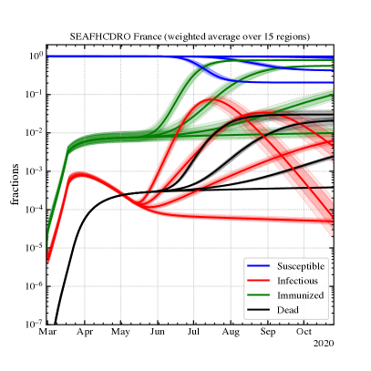
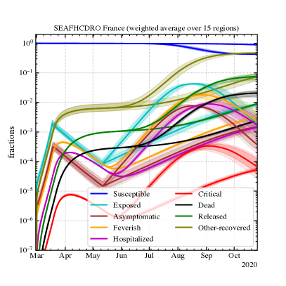
The French authorities have partially lifted the lockdown on 11 May 2020. This should, by itself, create more encounters and thus raise $R_{0}$. In the worst case, one would return to the pre-lockdown value of $R_{)}=3.4$. However, on the same date, face masks became widely available throughout the country. If a fraction $f$ of the population wears a face mask, then $R_{0}$ is multiplied by the factor $(1-f)^{2}$. It suffices that $1-1/\sqrt{3.4}$ = 46% of the population wears a face mask to bring $R_{0}$ below unity, and thus avoid a second wave, even without any social distancing.

Figure 17 illustrates four scenarios for the evolution of the pandemic in France after 11 May 2020, using pessimistic assumptions on $R_{0}$ where face masks are rarely used, with $R_{0}=1$, 1.2, 1.5, and 2. Note that these values lie between the low lockdown and the high pre-lockdown values of $R_{0}$.

The reader should first concentrate on the left panel of Figure 17, showing the evolution of the four super-phases. If $R_{0}=1$ after the partial lift of the lockdown, then the situation remains stable, and the number of Dead barely increases (by 10%). If, instead, the public mingles too much, leading to a high value of $R_{0}=2$, then the second wave will hit the country, with a peak of the Infectious super-phase in July and a multiplication by 20 of the number of Dead, reaching 3% of the population of Paris and of France as a whole, i.e., 2 million Dead! Note that the evolution for France as a whole mimics that of each region, i.e. Paris, because not only are the ratios of timescales to branching fractions are the same between regions, as before, but now the $R_{0}$ factors are also assumed the same. If the public chooses an intermediate path, with $R_{0}=1.5$, then the pandemic returns less dramatically than with $R_{0}=2$, and is delayed (as predicted by many with the SIR model). Still, with $R_{0}$ as high as 1.5 after the partial lifting of the lockdown, the number of deaths would rise to 2% of the population, i.e. over one million deaths! Finally, if $R_{0}=1.2$, then the pandemic rise is very slow at the start, with the number of Dead doubling only in August. But without stronger containment, this scenario would also lead to 0.25% of deaths in France, i.e. over 150 thousand. In other words, the time of doubling the total number of deaths in France on 11 May (26 thousand) is 1, 2, or 3 months if $R_{0}=2$, 1.5, or 1.2. The evolution of the pandemic is therefore highly sensitive to the value of $R_{0}$, with quiet evolution for $R_{0}=1$, manageable evolution for $R_{0}=1.2$, and increasingly fast second waves for $R_{0}=1.5$ and $R_{0}=2$.

It is useful to compare the evolution of Dead and of Infectious people. The dates when the number of Infectious will multiply by 5 compared to May 11 are May 25, June 10, and July 22, for $R_{0}=1.2$, 1.5, and 2, respectively. Similarly, the dates when the total number of Deaths in France will be multiplied by 5 (to reach 130 000) are June 28, July 31, and October 22, for $R_{0}=1.2$, 1.5, and 2, respectively. This means that the delay between Infectious and Dead super-phases is 34, 51, or 90 days, for $R_{0}=1.2$, 1.5, and 2, respectively.

The right panel of Figure 17, allows to obtain delays of the increase in Deaths with corresponding increases in earlier phases. The dates when the number of Hospitalized multiply by 5 since May 11, are June 12, and July 24, for $R_{0}=1.2$ and 1.5, respectively, i.e. very close to the dates of the Infectious in general. This is the consequence of the Feverish and Hospitalized dominating the Infectious super-phase on May 11, in contrast to the first-wave exponential growth when the Asymptomatic phase dominated the Infectious super-phase (see also Fig. 13). This is good news for the French authorities, as they can use hospital data to monitor the rise of deaths with over a month between the quintupling of hospitalizations and the quintupling of deaths, as long as $R_{0}\leq 2$.

6 Conclusions and Discussion

This work applies several epidemiological models to fit the French hospital data from March 19 to 4 May 2020. The evolution of hospitalizations and deaths after the national lockdown of 17 March was too slow to be compatible with the SIR model (Fig. 2). While the SEIHCDRO model (Fig. 4) provided an adequate fit to the hospital data, these data were better fit with the SEAFHCDRO model (Fig. 5), which splits the Infectious phase between one (Asymptomatic) that effectively contaminates Susceptibles and the following one (Feverish) whose members are too ill to leave their dwelling and contaminate Susceptibles. This better fit for SEAFHCDRO has higher Bayesian evidence, even after allowing for the extra two free parameters.

However, neither SEIHCDRO nor SEAFHCDRO can reproduce the rapid decrease in daily arrivals of Critical people at hospitals, which is more rapid than the corresponding decreases since lockdown in the daily Hospital arrivals, as well as daily Releases and Deaths (Figs. 7 and 8). I then introduced the SEAFHDRO model (Fig. 6) that merges the Critical and Hospitalized phases, but this model produced unsatisfactory results: 1) it fits less well the decrease in the daily Deaths compared to the SEAFHCDRO model; 2) it produces $R_{0}>1$ during lockdown for some regions.

This study produces the first analysis of ratios of timescales to branching fractions without resorting to the results of viral (PCR) testing. Such testing provides constraints on the timescales and branching fractions for the evolutionary paths $H\to C$, $H\to R$, $C\to D$, and $C\to R$, but not for previous paths, for which random testing is required. The results presented here indicate that the incubation phase lasts less than 5 days (Fig. 10), in agreement with many studies based on testing (e.g. Lauer et al., 2020). Moreover, this study produces the first geographic analysis of the $R_{0}$ factors, both before lockdown and during the lockdown. It indicates some regional differences, with Hauts-de-France and Paris showing higher $R_{0}$ before the lockdown, with a homogenization during the lockdown. Overall, the SEAFHCDRO model leads to $R_{0}=3.4\pm 0.1$ before and $R_{0}=0.65\pm 0.02$ during the lockdown (with 90% confidence limits, see Table 2), with some regional variations (Figs. 11 and 12). Therefore the national lockdown contributed to decreasing the basic reproduction number by a factor of roughly 5. The pre-lockdown value above is in good agreement with the values previously reported for France: $R_{0}=3.2\pm 0.1$ (Roques et al., 2020), $R_{0}=3.56$ (Unlu et al., 2020, without uncertainties), $R_{0}=3.0\pm 0.2$ (Di Domenico et al., 2020), and $R_{0}=3.3\pm 0.1$ and $3.4\pm 0.1$ for the two models of (Salje et al., 2020). Similarly, the lockdown value of $R_{0}$  during lockdown is in good agreement with previously reported values: $R_{0}=0.74$ (Unlu et al., 2020, with no uncertainties), $R_{0}=0.68\pm 0.06$ (Di Domenico et al., 2020), $R_{0}=0.47\pm 0.03$ (Roques et al., 2020), and $R_{0}=0.52\pm 0.03$ for both models of (Salje et al., 2020).

The SEAFHCDRO model also predicts the evolution of the 9 phases, and was also run in scenarios of no lockdown and partial lifting of the lockdown. The use of multiple-zone fits allows to accurately predict the early phases: Exposed, Asymptomatic and Feverish phases, which the single-zone models cannot do (Fig. 13). On 11 May 2020, the Feverish phase dominates the Infectious super-phase, followed closely by the Hospitalized, which both vastly outnumber the Asymptomatics who dominated the Infectious super-phase during the early pre-lockdown exponential growth (Fig. 13).

The time variations of the fractions (hence populations) of the different phases allow the measure of the fraction of Immunized, which is less than 1% throughout France and 3% in Paris (both with 95% confidence) with both the SEIHCDRO and SEAFHCDRO models (and 10 times less with SEAFHDRO). The first fraction is 4 times lower than the fraction of $4\pm 0.1\%$ found by Roques et al. (2020).

The IFR of France is estimated at 4$\pm$1%, i.e. 5 to 6 times higher than the previous estimates of Roques et al. (2020) and Salje et al. (2020). This difference may arise from incorrect assumptions on timescales and fractions by those two teams, or conversely by the lack of sufficiently strong priors on timescale to fraction ratios in the present analysis.

One should not be tempted by the argument that some fraction of people with high fever may still go out and contaminate Susceptibles. Indeed, the separation of Infectious into Asymptomatic and Feverish is precisely based on the assumption that what are called Feverish do not contaminate Susceptibles. In other words, by Feverish, one may think of people with very high fever, who will not only remain at home, but self-isolate from the other people in their dwelling.

Had there been no lockdown, nor social distancing, the COVID-19 pandemic would have resulted in over 2 million deaths in France (Fig. 16). Conversely, had the lockdown been enforced 10 days earlier, the number of deaths would have been 30 times lower. After May 11, the evolution will naturally depend on the value of the $R_{0}$ factor, which will be set by how well will people respect social distancing and on the fraction of people wearing facial masks. If nearly half of the population is masked, then $R_{0}$ should stay below unity and the pandemic will keep decreasing. On the other hand, if fewer than 46% of the population wear face masks, and assuming little social distancing, the pandemic will suffer a second wave (see Fig. 17). A value of $R_{0}$ as ‘low’ as 1.5 would produce disastrous consequences by the end of the Summer, if left unimpeded. But if France achieves $R_{0}=1.2$, it will have much more time to react to rises in hospitalizations.

There are several caveats to these results (the first few affecting many other similar studies). 1) Many deaths occur outside of hospitals, hence the dire deaths estimates of the models presented here are probably underestimates. 2) The models neglect Deaths of COVID-19 Hospitalized patients that were not sent to Critical care. 3) The models assume non-evolving ratios of timescales over branching fractions. However, the arrivals of Critical patients decreases faster than the SEAFHCDRO model predicts and the daily Deaths decreases faster than the models at late times, both suggesting that with time doctors have devised better protocols in handling COVID-19 patients without the need to send them to Critical care, and better treatment of the Critical care patients. 4) The analysis fails to follow the age distribution of the hospital data, whereas deaths by COVID-19 increase exponentially with age (as do regular deaths).

Nevertheless, it is hoped that this sort of analysis will present an example for future studies. It could be enhanced with better testing data, in particular regular random testing of a small fraction of the population, as well as other indicators of SARS-2 (e.g. the analysis of SARS-2 viruses in sewage Wurtzer et al. 2020).

References

- Centers for Disease Control and Prevention (2020) Centers for Disease Control and Prevention. What to do if you are sick, 2020. https://www.cdc.gov/coronavirus/2019-ncov/if-you-are-sick/steps-when-sick.html, extracted 10 May 2020.
- Di Domenico et al. (2020) Laura Di Domenico, Giulia Pullano, Chiara E. Sabbatini, Pierre-Yves Boëlle, and Vittoria Colizza. Expected impact of lockdown in île-de-france and possible exit strategies. medRxiv, 2020.04.13.20063933, 2020. doi: 10.1101/2020.04.13.20063933. URL https://www.medrxiv.org/content/early/2020/04/17/2020.04.13.20063933.
- Goodman and Weare (2010) Jonathan Goodman and Jonathan Weare. Ensemble samplers with affine invariance. Communications in Applied Mathematics and Computational Science, 5(1):65–80, January 2010. doi: 10.2140/camcos.2010.5.65.
- Hunter (2007) J. D. Hunter. Matplotlib: A 2d graphics environment. Computing in Science & Engineering, 9(3):90–95, 2007. doi: 10.1109/MCSE.2007.55.
- Lauer et al. (2020) Stephen A. Lauer, Kyra H. Grantz, Qifang Bi, Forrest K. Jones, Qulu Zheng, Hannah R. Meredith, Andrew S. Azman, Nicholas G. Reich, and Justin Lessle. The incubation period of coronavirus disease 2019 (covid-19) from publicly reported confirmed cases: Estimation and application. Annals of Internal Medicine, 172(9):577–582, 2020. doi: 10.7326/M20-0504. URL https://doi.org/10.7326/M20-0504. PMID: 32150748.
- Massonnaud et al. (2020) Clément Massonnaud, Jonathan Roux, and Pascal Crépey. Covid-19: Forecasting short term hospital needs in france. medRxiv, 2020.03.16.20036939, 2020. doi: 10.1101/2020.03.16.20036939. URL https://www.medrxiv.org/content/early/2020/03/20/2020.03.16.20036939.
- McKinney (2010) W. McKinney. Data structures for statistical computing in python. In Stéfan van der Walt and Jarrod Millman, editors, Proceedings of the 9th Python in Science Conference, pages 56 – 61, 2010. doi: 10.25080/Majora-92bf1922-00a.
- Roques et al. (2020) Lionel Roques, Etienne Klein, Julien Papaix, Antoine Sar, and Samuel Soubeyrand. Using early data to estimate the actual infection fatality ratio from covid-19 in france. medRxiv, 2020. doi: 10.1101/2020.03.22.20040915. URL https://www.medrxiv.org/content/early/2020/05/07/2020.03.22.20040915.
- Roques et al. (2020) Lionel Roques, Etienne K Klein, Julien Papaix, Antoine Sar, and Samuel Soubeyrand. Effect of a one-month lockdown on the epidemic dynamics of covid-19 in france. medRxiv, 2020.04.21.20074054, 2020. doi: 10.1101/2020.04.21.20074054. URL https://www.medrxiv.org/content/early/2020/04/24/2020.04.21.20074054.
- Salje et al. (2020) Henrik Salje, Cécile Tran Kiem, Noémie Lefrancq, Noémie Courtejoie, Paolo Bosetti, Juliette Paireau, Alessio Andronico, Nathanaël Hozé, Jehanne Richet, Claire-Lise Dubost, Yann Le Strat, Justin Lessler, Daniel Levy Bruhl, Arnaud Fontanet, Lulla Opatowski, Pierre-Yves Boelle, and Simon Cauchemez. Estimating the burden of sars-cov-2 in france. Science, 2020. ISSN 0036-8075. doi: 10.1126/science.abc3517. URL https://science.sciencemag.org/content/early/2020/05/12/science.abc3517.
- Unlu et al. (2020) Eren Unlu, Hippolyte Léger, Oleksandr Motornyi, Alia Rukubayihunga, Thibaud Ishacian, and Mehdi Chouiten. Epidemic analysis of covid-19 outbreak and counter-measures in france. medRxiv, 2020.04.27.20079962, 2020. doi: 10.1101/2020.04.27.20079962. URL https://www.medrxiv.org/content/early/2020/05/01/2020.04.27.20079962.
- van der Walt et al. (2011) S. van der Walt, S. C. Colbert, and G. Varoquaux. The numpy array: A structure for efficient numerical computation. Computing in Science Engineering, 13(2):22–30, 2011.
- Wurtzer et al. (2020) Sebastien Wurtzer, Vincent Marechal, Jean-Marie Mouchel, Yvon Maday, Remy Teyssou, Elise Richard, Jean Luc Almayrac, and Laurent Moulin. Evaluation of lockdown impact on sars-cov-2 dynamics through viral genome quantification in paris wastewaters. medRxiv, 2020. doi: 10.1101/2020.04.12.20062679. URL https://www.medrxiv.org/content/early/2020/05/06/2020.04.12.20062679.