Topology and axions in QCD

Abstract

QCD axions are at the crossroads of QCD topology and Dark Matter searches. We present here the current status of topological studies on the lattice, and their implication on axion physics. We outline the specific challenges posed by lattice topology, the different proposals for handling them, the observable effects of topology on the QCD spectrum and its interrelation with chiral and axial symmetries. We review the transition to the Quark Gluon Plasma, the fate of topology at the transition, and the approach to the high temperature limit. We discuss the extrapolations needed to reach the regime of cosmological relevance, and the resulting constraints on the QCD axion.

1 Overview

We know that strong interactions have many facets: among the most fascinating aspects there is the possibility of including a topological term into the QCD Lagrangian, which leads naturally to the prediction of a yet-unobserved particle – the QCD axion [1, 2, 3, 4] – a theoretically well-motivated candidate for Dark Matter. The same topological term solves an apparent mystery of the hadron spectrum, giving a mass to the $\eta^{\prime}$ meson [5, 6, 7].

Central in the discussions of this note is the relation between the axion mass $m_{A}$ and the axion decay constant $f_{A}$, which from the most recent estimates [8, 9] is

$$m_{A}=\frac{\sqrt{\chi_{top}}}{f_{A}}=56.9(5)\,\frac{10^{11}\text{GeV}}{f_{A}}~{}\text{$\mu$eV},$$ (1)

$\chi_{top}$ is the topological susceptibility of QCD, and the relation above is valid providing that $f_{A}$ is much larger than the QCD scale, $f_{A}\gg\Lambda_{QCD}$.

Astrophysical observations give the approximate limits $10^{12}\gtrsim f_{A}\gtrsim 4\times 10^{8}$ GeV; the upper bound prevents producing an amount of Dark Matter exceeding its estimated contribution, the lower one limits the amount of energy from the observed neutrino cooling of supernova SN1987A [10, 11, 12, 13, 14].

A range of decay constants $f_{A}$ exists for which the QCD axion would be a possible cold Dark Matter candidate[15, 16, 17, 18, 19, 20, 21]. This range has to be estimated by considering the axion’s cosmological history: in these analyses, the temporal evolution – or, equivalently, the temperature dependence – of the topological susceptibility in QCD plays an important role.

QCD can be studied in the framework of perturbation theory, and many important results have been obtained within this approach. However, it turns out that topology is completely outside the domain of perturbation theory: within a perturbative approach the contribution of the topological term would always be zero. Topology in QCD is related to the mechanisms of chiral and axial symmetries breaking and restoration. Chiral symmetry breaking at low temperatures, and instanton models combined with perturbation theory at very high temperatures, dictate the behaviour of the topological observables in these limiting situations [22, 23, 8, 9, 24].

At a temperature of about 150 MeV ($T_{c}=154(3)$ MeV according to the latest estimates [25]) chiral symmetry is approximatively restored, and quarks and gluons are in their plasma phase – the Quark Gluon Plasma. Temperatures ranging from $T_{c}$ till $\approx 2T_{c}$ are explored within experimental studies of Quark Gluon Plasma, higher temperatures – above 500 MeV – become relevant for cosmology, with strong interactions still playing a significant role. No analytic approach is quantitatively satisfactory for temperatures ranging from $T_{c}$ till $T\approx 2$ GeV. Within this range, ab-initio lattice simulations are mandatory.

High temperature lattice studies [26, 27, 28] face specific challenges: around the transition to Quark Gluon Plasma one has to deal with a pseudo-critical dynamics. At higher temperatures there are other challenges: lattice simulations are done on a discretized Euclidean space where the inverse of the (compactified) time direction $aN_{t}$ gives the temperature $T=1/aN_{t}$. With the current lattice spacings $a\simeq 0.05$ fm such high temperatures would mean three–four points in time directions: the space direction would get correspondingly small, while low lying modes would push the correlation lengths to large values, making finite size effects particularly dangerous. In addition to this, lattice topology [29, 30] poses specific problems. We will devote one Section to the discussions of QCD topology on the lattice and of the various methods that have been employed to address these issues. The final two Sections will present the current status of the results, with special attention to recent lattice works that for the first time addressed QCD axion physics from first principles[31, 32, 33, 34, 35, 36].

In this review we will only discuss the QCD axion. Let us just mention that axions’ physics is a much broader topic: axions appear in many different extensions of the Standard Model to explain the lack of observed CP violation of strong interactions. In string theories axions are ubiquitous, as they are generated by their complex topology [37]. In most (or all) models considered so far, axions are fundamental scalar fields, however recently models for composite axions have been considered as well [38, 39]. Axions are subjected to extensive experimental searches: experiments are optimized for certain mass ranges, and constraints from theories play an important role. For these important topics, which are not however in the scope of our discussion, we refer the reader to recent works and comprehensive reviews [13, 40, 20, 41, 42, 43, 44].

In brief summary, our discussion of topology and axions calls into play several entangled topics: QCD phenomenology, hadron spectrum, phases and phase transitions in QCD, early Universe and particle cosmology. At the same time, each of the two aspects – QCD topology and axions – has independent reasons of interest. We have thus organised the material trying to outline self-consistent discussions, with the aim to provide the basic information and tools to follow the current literature on QCD topology, and its implications on axion physics.

The material is organised as follows: in the next Section we will review the strong CP problem and introduce the axion. Section 3 discusses topology in the context of symmetries of QCD, the solution to the $U(1)_{A}$ puzzle and its role at the QCD transition. Section 4 is devoted to the main theoretical tool of this review, the lattice formulation. After a brief introduction, the focus is on the methods for topology. Next, we present the lattice results for the topological susceptibility at high temperature, and finally we discuss the impact of these results on axion physics.

2 Topology and the Strong CP problem

The QCD Lagrangian admits a CP violating term

$$\mathcal{L}={\cal{L}}_{QCD}+\theta\frac{g^{2}}{32\pi^{2}}F^{a}_{\mu\nu}\tilde{F}_{a}^{\mu\nu},$$ (2)

where $\dfrac{g^{2}}{32\pi^{2}}F^{a}_{\mu\nu}\tilde{F}_{a}^{\mu\nu}$ is the topological charge density $q(x)$, $\tilde{F}^{\mu\nu}=\dfrac{1}{2}\varepsilon^{\mu\nu\rho\sigma}{F}_{\rho\sigma}$, and $\theta\,q(x)$ is known as the $\theta$-term.

Without the $\theta$-term strong interactions conserve CP. Once this term is included, the neutron acquires an electric dipole moment $d_{n}$, which can be estimated with QCD sum rules: $d_{n}=2.4\times 10^{-16}\theta$ e cm [45] and chiral perturbation theory, $d_{n}=3.3\times 10^{-16}\theta$ e cm [46], and $d_{n}=3.6\times 10^{-16}\theta$ e cm[45]. The most recent experimental measure[47] of the neutron electric dipole moment is $d_{n}=(0.0\pm 1.1$ (stat) $\pm 0.2$ (sys)) $\times 10^{-26}$ e cm, which maybe interpreted as an upper limit $|d_{n}|<1.8\times 10^{-26}$ e cm at a $90\%$ C.L, leading to the bound $\theta<0.5\times 10^{-10}$. While the new results place more and more stringent limits, the unnaturally small value of $\theta$ has been known since long. This is known as the strong CP problem – we will come back to its solution in the next Section.

The Grand Canonical partition function of QCD is now a function of $\theta$. Moreover, for future discussion, we make explicit a dependence on the temperature $T$:

$$\mathcal{Z}(\theta,T)=\int\!\mathcal{D}[\varPhi]\,e^{-T\sum_{t}\int d^{3}x{\cal{L}}(\theta)}\ =e^{-VF(\theta,T)}.$$ (3)

Let us consider the $\theta$ dependent energy density $F(\theta,T)$ [48]. $F(\theta,T)$ is related with the probability of finding configurations with given topological charge $Q=\int d^{4}x\,q(x)$:

$$P_{Q}=\int\limits_{-\pi}^{\pi}\frac{d\theta}{2\pi}e^{-i\theta Q}e^{-VF(\theta)},$$ (4)

so the coefficients $C_{n}$ of the Taylor expansion

$$F(\theta,T)=\sum_{n=1}^{\infty}(-1)^{n+1}\frac{\theta^{2n}}{2n!}\,C_{n}$$ (5)

are given by the cumulants of the topological charge:

$$C_{n}=(-1)^{n+1}\frac{d^{2n}}{d\theta^{2n}}F(\theta,T)\Bigl{|}_{\theta=0}=\langle Q^{2n}\rangle_{conn}.$$ (6)

It can be shown that the free energy $F(\theta,T)$ as a function of $\theta$ has a minimum at $\theta=0$ [49]: however, this per se does not solve the strong CP problem, as at this stage $\theta$ is just a parameter.

It is convenient to introduce the dimensionless scaling function $f(\theta)$:

$$f(\theta,T)=(F(\theta,T)-F(0,T))/M^{4},$$ (7)

where $M$ is any suitable energy scale, for instance $\chi_{top}^{1/4}$. By comparing this with the Taylor expansion (5), it is natural to parametrize $f(\theta)$ as

$$f(\theta,T)=\frac{1}{2}C\,\theta^{2}s(\theta,T),$$ (8)

where $s$ is a dimensionless function, and $s(\theta\!=\!0)=1$. Then

$$s(\theta,T)=1+b_{2}(T)\theta^{2}+b_{4}(T)\theta^{4}+\ldots,$$ (9)

and the $b$’s are easily expressed in terms of the cumulants $C_{n}$ in Eq. (6).

At zero and low (below or around $T_{c}$) temperatures $F(\theta,T)$ can be computed by considering low energy effective Lagrangians [50, 51] – these are actually the calculations leading to the estimate of the neutron magnetic dipole moment mentioned above. A recent study improved the precision by including electromagnetic corrections and NNLO corrections in the chiral expansion [9]. The topological susceptibility and the fourth-order cumulant have been computed up to NNLO in $U(3)$ Chiral Perturbation Theory[52] at zero and non-zero temperature, as well as within Interacting Instanton Liquid Models [53, 18]. Finite temperature corrections have been computed [8, 24], and their validity stretches till $T\simeq T_{c}$.

In the Quark Gluon Plasma phase the basic expression for $F(\theta,T)$ was computed long ago[22, 23]. The dilute gas approximation (DIGA) and high temperature perturbation theory at leading order reads[22, 23]:

$$F(\theta,T)-F(0,T)\simeq T^{4-\beta_{0}}\left({\frac{m_{l}}{T}}\right)^{N_{f,l}}(1-\cos\theta),$$ (10)

where $\beta_{0}=11N_{c}/3-2N_{f}/3$ and $N_{f,l}$ is the number of light flavors.

The fundamental physical fact[22] is that at sufficiently high temperature only fields with integral topological charge can contribute to the functional integral, so the $\theta$ dependence of the free energy at high temperature is dominated by instantons – ultimately only by the ones with positive or negative unit charge. This contrasts with low temperature, where the physics mechanisms leading to a contribution of the topological $\theta$ term to the partition function can be understood without invoking instantons [54]. The microscopic behaviour of the plasma close to phase transition, its interpretation in terms of physical degrees of freedom, including topological structures, is of course a subject of active research [55, 56, 57].

As already mentioned, the main tool to analyze strong interactions in non-perturbative regime is lattice simulations, which rely on a sampling of the phase space weighted with the $e^{-S}$, where $S$ the Euclidean action. In Euclidean space-time the Minkowskian Lagrangian (2) becomes complex for real values of $\theta$: this hampers a direct importance sampling. However, it is possible to consider a Taylor expansion around $\theta$ = 0 – cf. Eqs. (6) and (9) – thus monitoring the approach to one of the limiting expressions for $F(\theta,T)$[22, 8, 9]. Clearly this approach is satisfactory only at small $\theta$. For instance, the interesting physics around $\theta=\pi$ [58] would require a different approach. Some attempts in this direction have been made [59] by using an imaginary value of $\theta$, followed by an analytic continuation to real values. The topological susceptibility, whose computations will be described in the following, is the leading order contribution to this series.

2.1 Solution of the strong CP problem: the axion

Suppose $\theta$ in Eq. (2) were a dynamical parameter: in such a case, dynamics would force its value to zero, thus solving the strong CP problem. In order to achieve this, the existence of an extra particle [1, 2, 3, 4] was postulated, a pseudo-Goldstone boson of a spontaneously broken symmetry known as the Peccei-Quinn (PQ) symmetry, which couples to the QCD topological charge, with a coupling suppressed by a scale $f_{A}$. The axion field $a(x)=f_{A}\theta(x)$ is now a space-time dependent $\theta$ parameter. The axion–QCD Lagrangian reads

$$\mathcal{L}={\cal{L}}_{QCD}+\theta\frac{g^{2}}{32\pi^{2}}F^{a}_{\mu\nu}\tilde{F}_{a}^{\mu\nu}+\\ {\partial^{2}_{\mu}}{a^{2}}+\frac{a}{f_{A}}\frac{g^{2}}{32\pi^{2}}F^{a}_{\mu\nu}\tilde{F}_{a}^{\mu\nu}.$$ (11)

Moreover, one assumes that the theory enjoys a shift symmetry: $a\to a+\alpha$. The $\theta$ angle may be eliminated by a shift, and the $\theta$ dependence has been traded with a dependence on the axion field, whose minimum is at zero [49]: this solves the strong CP problem. Besides the original papers [1, 2, 3, 4], there are many reviews discussing this point detail[60, 48].

$F(\theta,T)$ can now be used to compute the axion mass. At leading order in $1/f_{A}$ – well justified as $f_{A}\gtrsim 4\times{10^{8}}$ GeV – the axion can be treated as an external source, and its mass is given by

$$m_{A}^{2}(T)f_{A}^{2}=\frac{\partial^{2}F(\theta,T)}{\partial\theta^{2}}\biggl{|}_{\theta=0}\equiv\chi_{top}(T)\;.$$ (12)

At low temperature, chiral perturbation theory gives the result [3]

$$m_{A}^{2}=\frac{m_{u}m_{d}}{(m_{u}+m_{d})^{2}}\frac{m_{\pi}^{2}f_{\pi}^{2}}{f_{A}^{2}},$$ (13)

which has been recently improved to NLO [8]. Finite temperature corrections have been computed[8, 9] – the analysis is the same as the one discussed above for QCD topology – and their validity stretches till $T\simeq T_{c}$.

At low temperature the LO chiral perturbation theory relation between topological susceptibility and chiral condensate [58] ensures that the two expressions coincide. More generally, we have now a prescription for the temperature dependence of the QCD axion mass. We underscore that the axion is massive because the $U(1)$ PQ symmetry is anomalous: because of that, the would-be Goldstone is a massive pseudo-Goldstone scalar. The amount of breaking is regulated by the topological susceptibility, hence it is temperature dependent, and there is a close relation with chiral symmetry.

In very brief summary, the essence of this discussion is the close relation between axion mass and topological susceptibility:

$$m_{A}^{2}f_{A}^{2}=\chi_{top},$$ (14)

which is valid for any temperature. Inserting the known value of today’s topological susceptibility, we obtain Eq. (1).

3 Topology, symmetries and spectrum of strong interactions

We have seen that a relation emerges, which links topological susceptibility and chiral condensate, and that the axion is massive if the topological susceptibility is non-zero. We will see that a completely analogous mechanism solves another puzzle in QCD, the $U(1)_{A}$ problem. In essence, without a contribution from the $\theta$-term, all isoscalar mesons should be lighter that $\sqrt{3}\,m_{\pi}$. It turns out that the same anomaly giving mass to the axion is responsible for solving this problem.

The rich behaviour of the strong interactions is encoded in the apparently simple QCD Lagrangian

$${\cal{L}}=\sum_{a=1}^{n}\bar{q}_{La}\not{\partial}{q}_{La}+\bar{q}_{Ra}\not{\partial}{q}_{Ra}-m(\bar{q}_{La}q_{La}+\bar{q}_{Ra}{q}_{Ra})+\theta\,\frac{g^{2}}{32\pi^{2}}F^{a}_{\mu\nu}\tilde{F}_{a}^{\mu\nu}+{\cal{L}}_{gauge},$$ (15)

where $q$ are the quark fields and $q_{L,R}=\dfrac{1\mp\gamma_{5}}{2}q$. In this form, and with $m=0$, the invariance under the transformation $q_{L}\to V_{L}q_{L}$, $q_{R}\to V_{R}q_{R}$, with $V\in U(n)$, is manifest. Thus, at classical level there is a global symmetry $U(n)_{L}\!\times\!U(n)_{R}\cong SU(n)\!\times\!\ SU(n)\!\times\!U(1)_{V}\!\times\!U(1)_{A}$. The pseudoscalar mesons are candidate Goldstone bosons if the symmetry $SU(n)\!\times\!SU(n)$ is spontaneously broken. With finite masses we have to consider approximate symmetries, either $SU(2)\!\times\!SU(2)$, assuming that the strange quark does not contribute to chiral dynamics, or $SU(3)\!\times\!SU(3)$ including it. The pion triplet has masses of about $140$ MeV, the meson containing strange quarks $\eta$ about $540$ MeV, the four $K$’s at about $400$ MeV, and finally the $\eta^{\prime}$ much heavier, $960$ MeV. The most natural scenario accommodating experimental observations of pions and $K$ mesons is the spontaneous breaking of the $SU(3)\!\times\!SU(3)$ symmetry. This breaking should be accompanied by the formation of a quark condensate, which, in turn, would spontaneously break $U(1)_{A}$. Hence $\eta^{\prime}$ should follow the same fate as the other mesons, which clearly it is not the case. The way out is a breaking of the $U(1)_{A}$ symmetry[7]: the same topological structures which are responsible for the axion mass give mass to the $\eta^{\prime}$. With the $q_{L}\to e^{-i\theta}q_{L}$, $q_{R}\to e^{i\theta}q_{R}$ violation, the remaining symmetry is then $U(n)_{L}\!\times\!U(n)_{R}/U(1)\cong SU(n)\!\times\!SU(n)\!\times\!U(1)_{V}$. The experimental value of the $\eta^{\prime}$ mass gives an experimental evidence to the explicit $U(1)_{A}$ breaking.

Theoretically, the breaking can be explored by lattice simulations. The topological contribution to $\eta^{\prime}$ mass is given by the Witten-Veneziano formula [61, 54, 62]:

$$\chi_{top}\Bigl{|}_{N_{f}=0}=\frac{1}{2N_{f}}f_{0}^{2}\left(m_{\eta^{\prime}}^{2}+m_{\eta}^{2}-2m_{K}^{2}\right),$$ (16)

where $\chi_{top}$ has to be calculated in pure Yang-Mills theory corresponding to the quenched limit $N_{f}=0$ of QCD. Note that in the chiral limit both $\eta$ and $K$ masses in the r.h.s. of Eq. (16) vanish. The topological susceptibility is accessible in lattice simulations (see Section 4 for details), and the relation (16) was confirmed on the lattice with high accuracy [63, 64, 65]. So, it is safe to declare that the solution to the $U(1)_{A}$ problem has been confirmed also by these ab initio studies. The natural question then arises, concerning the interrelation of chiral and axial symmetries at finite temperature, and the fate of the $\eta^{\prime}$, a central issue of strong interaction physics which is addressed by model studies [52, 66], phenomenological analysis [67, 68, 69], FRG studies [70, 53, 71], and mostly by lattice analysis [72, 73, 74, 75, 76, 77, 78, 79].

The fate of $U(1)_{A}$ has implications on the nature of the chiral phase transition. If the axial symmetry breaking is not much sensitive to the chiral restoration, the breaking pattern is indeed $SU(2)_{L}\!\times\!SU(2)_{R}\to SU(2)_{V}$ or $O(4)\to O(3)$ symmetry[80]. In this case the universality class is well known, and would correspond to a second order transition with known exponents and equation of state. Alternatively, if the axial symmetry is effectively restored at the same temperature (it cannot be restored before) as the chiral transition, then the relevant symmetry would be $U(2)_{L}\!\times\!U(2)_{R}\to U(2)_{V}$, which would hint either at a first or even a second order transition with different exponents [81].

Lattice simulations can be performed with varying values of quark masses. When addressing the issue of the universality class of the transition one takes advantage of this possibility to study the associate mass dependence: different universality classes have distinct predictions for the mass dependence of the transition temperature. In principle, the universality class of the transition, as well as the critical temperature in the chiral limit, could be inferred by contrasting lattice results with theoretical predictions [27, 26, 25]. One typical choice is the pseudocritical temperature as a function of the quark mass $T_{c}(m_{\pi})$, which within the scaling window of the theory should follow

$$T_{c}(m_{\pi})=T_{c}(0)+A\,m_{\pi}^{2/{\beta\delta}}.$$ (17)

In practice, the exponents characterizing different critical behaviours change very little: $2/\beta\delta\approx 1.08$ for $O(4)$ and $2/{\beta\delta}\approx 1.28$ for a $Z_{2}$ universality class associated with a hypothetical endpoint of a first order transition in the chiral limit[82]. The current status of the QCD transition is shown in Figure 1. The heavier quark mass is at its physical value, and we read off from the plot the accepted value of the pseudo-critical temperature of the QCD crossover: $T_{c}=154.3(2)$ MeV. The fit to the data is consistent with an $O(4)$ transition, but others cannot be ruled out[25, 27].

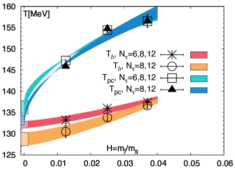
Figure 1: The pseudo-critical temperatures from HotQCD from different observables, and their extrapolation to the chiral limit from a recent review [28] (see also[25]).

Results from Wilson fermions exist as well, and confirm this picture[78, 79, 83]. Besides giving information on the possible universality classes, and on the physical transition, Figure 1 shows the critical temperature in the chiral limit – a genuine singular point of strong interactions. This temperature marks the beginning of the Quark Gluon Plasma and the high temperature phase of QCD.

More direct approaches to the analysis of the breaking and restoration of chiral symmetry based on the consideration of (approximate) order parameters or Dirac spectrum have not been conclusive regarding the fate of the $U(1)_{A}$ symmetry. The main observable characterizing chiral symmetry is the chiral condensate, the order parameter of the $SU(2)\!\times\!SU(2)$ symmetry. When analyzing axial symmetry, it is useful to consider a fuller set of chiral observables associated to vector and axial symmetries: one can consider the correlation functions of local operators[69, 84]

$$\sigma = \bar{\psi}_{l}\psi_{l}$$

$$\delta^{i} = \bar{\psi}_{l}\tau^{i}\psi_{l}$$ (18)

$$\eta = i\bar{\psi}_{l}\gamma^{5}\psi_{l}$$

$$\pi^{i} = i\bar{\psi}_{l}\tau^{i}\gamma^{5}\psi_{l}.$$

$(\sigma,\pi^{i})$ and $(\eta,\delta^{i})$ are related by $SU(2)_{L}\!\times\!SU(2)_{R}$ transformations, $(\sigma,\eta)$, $(\delta^{i},\pi^{i})_{1\leq i\leq 3}$ via $U(1)_{A}$. Inspecting the degeneracy, or lack thereof, of these two point functions, or, equivalently, of the associated susceptibilities (integrals over the four space) one accesses information on the realization of symmetries. First results including the $\eta^{\prime}$ have appeared recently[78, 79]. The analysis is complicated by the explicit breaking induced by the quark mass, by the ultraviolet divergences of the susceptibilities, and by the possible occurrence of accidental degeneracies [85]. Despite these difficulties, there is consensus that axial symmetry is effectively restored above $T_{c}$, say $T\simeq 1.2T_{c}$ [86, 72, 84, 87, 88, 89, 77, 90, 91, 92, 93, 77], however it is unclear how close to $T_{c}$ the effective restoration may happen. There are also attempts to tackle this issue within a first-principle FRG approach [94], but at the moment the interrelation of chiral and $U(1)_{A}$ restoration remains an unresolved problem of QCD.

As already stressed, the anomaly effects breaking the $U(1)_{A}$ symmetry are related to the topological properties of QCD, so these uncertainties further add to the interest of topological studies. At a more practical level, the restoration of the $SU(2)\times SU(2)$ opens the way to a simple measurements of the topological susceptibility at high temperatures. We will return to this point in the next Section.

4 Lattice Field Theory: methods and results

4.1 Lattice QCD: brief introduction

The essentially nonperturbative nature of topology and related issues renders the usual perturbative methods of quantum field theory to be of limited use, so alternative approaches are required. Currently, one of the most prospective and rewarding approaches is lattice formulation of QCD, which allows first-principle calculation of topological and other physical quantities in numeric simulations. In Lattice QCD the continuous spacetime is replaced by discrete 4D Euclidean lattice, and so discretized versions of operators defined on sites of the lattice are introduced. Then, expectation value of observable $O$ can be defined as

$$\langle O\rangle=\frac{1}{Z}\int\!\mathcal{D}[U]\,e^{-S_{lat}[U]}O[U],$$ (19)

where

$$Z=\int\!\mathcal{D}[U]\,e^{-S_{lat}[U]}$$ (20)

is discretized partition function (3), and $S_{lat}$ is lattice action based on the continuum QCD Lagrangian. One of the key parameters is number of lattice points in space (time) directions $N_{s}$($N_{t}$) and lattice spacing $a$ between two consequent points. In modern simulations, the values $N_{s}=128$ and $N_{t}=256$, or even higher, are reached, with lattice spacings of order $a\sim 10^{-2}-10^{-1}$ fm.

The integrals in Eqs. (19)–(20) are taken over all lattice gauge variables $U$, totaling up to $\mathcal{O}(N_{s}^{3}N_{t})$ integration variables. With direct evaluation being obviously impossible, a numerical approximation is applied:

$$\langle O\rangle\approx\frac{1}{N}\sum_{i}O[U^{(i)}],$$ (21)

where the set of lattice configurations $U^{(i)}$, $i=1,\ldots,N$ are generated by means of Monte Carlo algorithm to satisfy probability distribution $\propto e^{-S_{lat}[U]}$. Note that the error of approximation (21) decreases with the number of generated configurations $N$ as $\mathcal{O}(1/\sqrt{N})$.

From practical point of view, the main drawback of the outlined approach is that the realistic simulations, especially at physical quark masses, consume considerable computational resources, so vast allocations at, in general, supercomputer facilities are required. Also, direct lattice simulations are not possible in some physically interesting cases, such as QCD with finite chemical potential or non-zero $\theta$-term, since the weighting factor $e^{-S_{lat}[U]}$ becomes complex-valued and cannot serve as probability measure anymore.

From theoretical point of view, the way to discretize QCD operators on the lattice, including lattice action $S_{lat}$ itself, is not unique. This leads to several possible options, each with their own advantages and drawbacks, with the arising discretization artifacts (also called lattice artifacts due to their origin in finiteness of lattice spacing $a$) to be dealt in controllable way. In general, it is feasible to have several lattice calculations based on different choices of lattice action, cross-checking and compensating each other, in order to have solid and well-understood physical results. The constant progress in theoretical methods, simulation algorithms and hardware efficiency has already made such cross-checks possible, with physical $N_{f}=2+1+1$ quark masses reached in several independent studies [95, 32, 96, 97]. For more details on lattice field theory, fermionic discretizations and corresponding subtleties we refer to comprehensive presentations in Refs. [98, 99, 100, 101, 102].

4.2 Topological charge on the lattice

Topology on the lattice can be measured by several methods. Let us start from the so-called gluonic definition, which is based on continuum definition for topological charge density in pure gluonic Yang-Mills theory:

$$q(x)=\frac{1}{32\pi^{2}}\varepsilon_{\mu\nu\rho\sigma}\mathop{\mathrm{Tr}}\nolimits[F^{\mu\nu}(x)F^{\rho\sigma}(x)],$$ (22)

where $F^{\mu\nu}(x)$ is continuous field strength tensor. Then, the topological charge is defined as

$$Q=\int\!q(x)\,d^{4}x.$$ (23)

It can be shown (see, e.g., [103]), that $Q$ equals to the so-called Pontryagin index or winding number of gauge fields, which can only assume integer values.

The definitions (22)–(23) are straightforwardly implemented on the lattice:

$$Q=\frac{a^{4}}{32\pi^{2}}\varepsilon_{\mu\nu\rho\sigma}\sum_{n}\mathop{\mathrm{Tr}}\nolimits[F_{lat}^{\mu\nu}(n)F_{lat}^{\rho\sigma}(n)],$$ (24)

where summation is over all sites of the lattice. The discretized field strength tensor can be simply evaluated as traceless antihermitian part of the elementary plaquette $U_{\mu\nu}$, $F_{lat}^{\mu\nu}\propto U_{\mu\nu}\bigl{|}_{\footnotesize\begin{smallmatrix}\text{\!\!\!traceless}\\ \text{antiherm.}\end{smallmatrix}}\equiv(U_{\mu\nu}-U^{\dagger}_{\mu\nu})-\frac{1}{3}\mathop{\mathrm{Tr}}\nolimits(U_{\mu\nu}-U^{\dagger}_{\mu\nu})$, and vast majority of improvements with respect to the terms of higher order in lattice spacing $a$ are possible [104, 105]. The plaquette $U_{\mu\nu}$ represents product of four oriented gauge variables forming closed loop on the lattice:

$$U_{\mu\nu}(n)=U_{\mu}(n)U_{\nu}(n+\hat{\mu})U^{\dagger}_{\mu}(n+\hat{\nu})U^{\dagger}_{\nu}(n),$$ (25)

where $U_{\mu}(n)$ denotes gauge variable at the site $n$ pointing along the $\hat{\mu}$ axis.

Still, it turns out that even with highly improved definitions of $F_{lat}^{\mu\nu}$, the topological charge calculated on the lattice from Eq. (24) is non-integer. The reason, along with the lattice artifacts, is ultraviolet fluctuations of gauge variables, which have to be additionally renormalized. The alternative is to ”smooth” UV fluctuations in gauge fields prior to applying definition (24) directly, for which many methods have been used: cooling and over-improved cooling [104], different smearing techniques [106, 107, 108] and other smoothing algorithms [29]. One of the recent approaches is smoothing by gradient flow [109], which has prominent advantage of its renormalization properties proven at all orders in perturbation theory [110], making it theoretically better established than other methods.

The gradient flow is applied to gauge variables by differential equation

$$\dot{V}_{\mu}(n,\tau)=-g^{2}[\partial_{n,\mu}S_{G}(V(\tau))]V_{\mu}(n,\tau),\qquad V_{\mu}(n,0)=U_{\mu}(n),$$ (26)

where flow time $\tau$ determines the amount of smoothing. Gradient flow can be based on arbitrary choice of gauge action $S_{G}$ in (26), although the simplest Wilson gauge action is mostly used. On practice, Eq. (26) is solved by standard numerical methods for differential equations, such as Runge–Kutta scheme [109].

It was shown [111, 112, 113], that in leading order of perturbation theory cooling, smearing and gradient flow lead to the identical result for an updated gauge variable, allowing to derive a relation between flow time $\tau$ and number of cooling/smearing steps. Moreover, numerical measurements revealed that even with relatively large amount of smoothing applied, all considered methods give highly correlated and, in most cases, almost identical results in both zero and finite temperature studies [111, 114, 112, 113, 115, 116]. For illustration, we show in Figure 2 comparison of typical Wilson cooling and gradient flow histories for topological charge of a single lattice configuration. In Figure 3 we calculate the topological susceptibility

$$\chi_{top}=\frac{\langle Q^{2}\rangle}{V},\qquad V=a^{4}N_{s}^{3}N_{t}$$ (27)

by averaging squared topological charge $Q^{2}$ on the sets of configurations at different temperatures and compare four methods: Wilson flow and cooling with over-improved stout-link smearing and cooling [116].

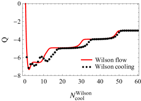
Figure 2: Wilson cooling and gradient flow histories for topological charge of a single lattice configuration. $N^{\text{Wilson}}_{\text{cool}}$ denotes number of cooling steps.

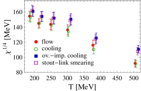
Figure 3: Topological susceptibility $\chi_{top}\propto Q^{2}$ calculated by four different smoothing methods at finite temperature [116].

Another approach to topology on the lattice is established by Atiyah-Singer index theorem [117, 118]

$$\frac{1}{32\pi^{2}}\,\varepsilon_{\mu\nu\rho\sigma}\!\int\mathop{\mathrm{Tr}}\nolimits[F^{\mu\nu}(x)F^{\rho\sigma}(x)]\,d^{4}x=n_{+}-n_{-}$$ (28)

relating topological charge to the number of zero modes of the massless Dirac operator with positive and negative chirality $n_{\pm}$. Eq. (28) remarkably connects a purely gluonic quantity with the properties of fermionic operator, so it is called the fermionic definition of topological charge. A principal possibility to implement the Dirac operator satisfying theorem (28) on the lattice was proven in [119], and Neuberger’s implementation of overlap Dirac operator [120, 121] is most commonly used on practice.

The fermionic definition (28) is appealing in many ways: it has a solid theoretical basis, not affected but UV fluctuations (no prior smoothing of gauge fields needed) and provides integer values of $Q$ by design. The main drawback, however, is very high computational cost of calculating low-lying modes for any implementation of massless Dirac operator on the lattice. As an alternative, one can consider Wilson–Dirac spectral flow [122] and stochastic spectral projector [123, 124] approaches, which are still closely related to the definition (28).

Finally, a simple (although, only approximate) way to express the topological susceptibility (27) through fermionic observable was outlined in Refs. [125, 126, 84] on the basis of QCD symmetry relations. In the continuum theory,

$$\frac{1}{32\pi^{2}}\,\varepsilon_{\mu\nu\rho\sigma}\!\int\mathop{\mathrm{Tr}}\nolimits[F^{\mu\nu}(x)F^{\rho\sigma}(x)]\,d^{4}x=m_{l}\int d^{4}x\,\bar{\psi}(x)\gamma_{5}\psi(x),$$ (29)

where $m_{l}$ is the light quark mass. By squaring Eq. (29) and averaging over gauge fields, we immediately get

$$\chi_{top}=\frac{\langle Q^{2}\rangle}{V}=m_{l}^{2}\,\chi_{5,disc}.$$ (30)

The disconnected pseudo-scalar susceptibility $\chi_{5,disc}$ is known to suffer from large fluctuations, so its direct calculation is cumbersome. Instead, we can utilize the fact that with restoration of chiral symmetry $\chi_{5,disc}$ becomes equal to the disconnected chiral susceptibility $\chi_{disc}$. Then, we finally arrive to

$$\chi_{top}(T\gtrsim T_{c})=m_{l}^{2}\,\chi_{disc}=m_{l}^{2}\,\frac{V}{T}\left(\langle{(\bar{\psi}\psi)^{2}}\rangle_{l}-\langle{\bar{\psi}\psi}\rangle_{l}^{2}\right).$$ (31)

On the lattice, discretization artifacts have to be taken into account, so Eqs. (29)–(31) hold only approximately. Moreover, Eq. (31) allows to calculate topological susceptibility only in chirally-symmetric phase, i.e. at sufficiently high temperatures. Still, it turned out to be quite useful [33, 36], since the chiral condensate $\langle{\bar{\psi}\psi}\rangle_{l}$ is easily accessible in lattice calculations, and high-temperature behaviour of $\chi_{top}$ is of great importance to axion physics, as we discuss in details in Section 6.

The extensive study and comparison of the different methods for topological charge on the lattice have been carried out in Refs. [115, 113]. We present in Figure 4 the summarizing plot from Ref. [113] containing overall comparison of various gluonic and fermionic definitions outlined above. All definitions show from good to perfect agreement between themselves, except for gluonic definition (24) without any prior gauge field smoothing (# 7 in Figure 4) and spectral projector results (# 5 and 6). As was discussed above, direct measurements with Eq. (24) are meaningless due to the large UV fluctuations in unsmoothed gauge fields, which is directly confirmed in Figure 4. Regarding spectral projectors, less correlated with gluonic and even other fermionic methods, we note that for measurements on finite lattices perfect matching between different definitions is not really expected, even for the methods theoretically proven to be identical, due to $\mathcal{O}(a)$ lattice artifacts. It was shown in Ref. [127] that in continuum limit $a\to 0$ the topological susceptibility calculated with gradient flow agrees with the results from spectral projectors (obtained, though, by direct numerical evaluation of eigenmodes, not stochastically estimated), with the latter actually much less contaminated by cut-off effects.

Figure 4: Correlation matrix between different gluonic and fermionic definitions of topological charge [113].

5 Topology in the Plasma

In this Section we present the results for topology at nonzero temperature, above the QCD transition, see Figure 1, from lattice simulations. In the pseudo-critical region the results for the topological susceptibility complement the analysis of the transition of Section 3: at higher temperature strong interactions approach a perturbative regime, which for topology is described by DIGA instanton models. It turns out that the topological susceptibility has a very intricate temperature dependence around the transition. It has an exponent very different from the DIGA predictions – we will see that in QCD the DIGA predictions are approached only above $T=350$ MeV. Clearly these different behaviours highlight the role of different topological objects dominating the QCD partition function at high temperature, and of their interactions [55, 56, 128]. We will then contrast the lattice results with the predictions for $F(\theta,T)$ from the DIGA and high temperature perturbation theory (10). Besides giving information on the nature of the QCD vacuum, this parametrization, if valid, allows the extrapolation to larger temperatures.

5.1 Only gluons: the Yang-Mills theory

Due to its relative simplicity, a theory with only gluons is used as a laboratory for new ideas. Moreover, stable and controlled results in the quenched model are an important proof of principle of the feasibility of calculations in the realistic case.

The first pioneering studies of finite topology in Yang-Mills theory on the lattice[129] were based on the gluonic definition. One of the first, if not the first, large scale analysis of the topological susceptibility at high temperature based on the index theorem appeared a few years later[130]. The results covered the range $0.8T_{c}<T<1.5T_{c}$.

Berkowitz, Buchoff, and Rinaldi [31] were the first ones to implement the suggestion of Ref. [18] to use lattice results as a quantitative input to axion cosmology. This motivated a study in an extended range of temperatures. They used the gluonic definition for the topological charge with suitable cooling to obtain results up to $T\simeq 700$ MeV. Smoothing procedures and multiple volumes were used to control systematic errors, although a clear continuum extrapolation was not performed. The results were fitted to the DIGA motivated power law decay $\chi(T)=A\,T^{b}$, with a quoted value of the exponent $b=-5.64(4)$.

In Ref. [131] the topological susceptibility was measured in the even larger temperature interval $0.9<T/T_{c}<4$, for several lattice spacing, thus allowing a controlled continuum extrapolation. The quoted result by [131] is $\chi(T)=0.11(2)(1)(T/T_{0})^{b}$, $T_{0}=1.02(5)(2)$ ($T_{0}$ should be 1 in unit of $T_{c}$), $b=-7.1(4)(2)$. The exponent is in nice agreement with the DIGA result, whereas the overall normalization of the DIGA prediction still differs from the lattice results by a factor of order ten. The same group confirmed these results in a later study[32].

Two more recent studies focused on selected large temperatures, implementing some methodological refinements: master-field simulations of the $SU(3)$ gauge theory, leading to high accuracy estimates [132], and improved reweighting [133, 134], allowing estimated for temperatures as high as $7\,T_{c}$.

In Figure 5 we superimpose the numerical results [31] with the central values of the fit [131]. In the same plot we show the 2002 results [130] and the more recent ones [132, 133] (omitting the larger temperature in the latter case), obtained by use of master field simulations and improved reweighting. Interestingly, there is a good agreement up to $T/T_{c}\simeq 1.5$. The fit[31], available in the limited temperature range, gives $b=-5.64(4)$ – rather stable with respect to changing the interval. In [131] the quoted result is $b=-7.1(4)(2)$, where the systematic error comes from fits with different initial points $T/T_{c}[1.3-1.7]$. We have checked that the results[31] appear to be stable with sliding the fit interval, hence a plausible source for the (small) discrepancy may come from residual finite spacing. Indeed, either Refs. [131] and [133] consistently find a decreasing trend with extrapolations, with errors which may be of the order of several percent.

From the point of view of lattice results, the emerging scenario is rather pleasing: different groups using different techniques find a nice agreement once the continuum extrapolation is taken into account. The continuum extrapolation seems more critical, in agreement with general discussions on lattice topology, at higher temperatures, while around $T_{c}$ finite spacing effects seem to be less severe. Master-field simulations afford an unprecedented accuracy for topological calculations, however the authors themselves note that at temperatures higher than the ones considered here, master-field simulations of topological susceptibility must be expected to be increasingly sensitive to lattice spacing[132]. It would be very nice to have results at even higher temperatures, though, in order to probe more convincingly the approach to the DIGA limit, which remains a subtle issue.

Let us stress, as noticed[131], that the strong coupling constant, at the relevant thermal scale of $2\pi T$ is still sizeable in the considered range of temperatures. If we monitor the approach to DIGA via the exponenent value, we may conclude that the results are rather close to this regime: the fit estimate [131] is indeed $b=-7.1(4)(2)$. The approach to the DIGA result appears even faster than RG prediction[131]: an improved estimate of $b$ shows a mild consistent increase in the range $1.5<T/T_{c}<5$, and the DIGA exponent appears to be approached from below. Looking at the data, we note that close to $T_{c}$ we have instead a rather fast drop of the topological susceptibility, perhaps reflecting the fast transition from the confined to the deconfined phase at the $SU(3)$ (weak) first order transition. Putting all together, we may expect a fast decrease of the apparent $b$ exponent immediately above $T_{c}$, then a mild increase approaching the DIGA limit. If these two behaviours are smoothly connected, probably it is not surprising to observe a proximity to the DIGA results also at moderate temperatures – which although may be merely accidental.

When looking at the absolute value of the susceptibility, one clearly finds a large deviation from the DIGA prediction, by about one order of magnitude[131]. While such large deviations are not uncommon in perturbative QCD, they indicate that the DIGA limit has not been completely reached yet. However, Ref. [131] have also studied higher order terms in the potential, analyzing the coefficient $b_{2}$ in the expansion, which appears to approach the DIGA limit, even faster than the susceptibility.

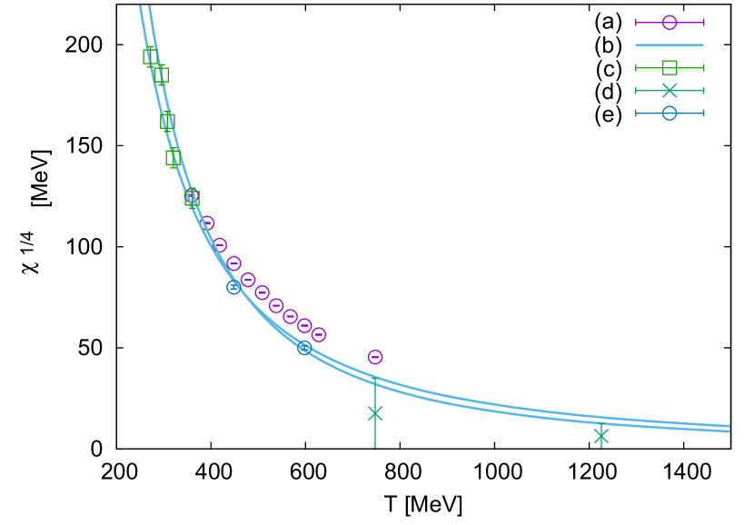
Figure 5: The fourth root of topological susceptibility versus the temperature for the Yang-Mills studies reviewed here. Only a representative subset of the results are shown. (a) is from Ref. [31], Table I. (b) uses the final fits reported in [131]. (c) is the earlier results of [130], (d) the results from improved reweighting [133] and (e) from the master fields simulations [132], see text for details.

5.2 Quark-Gluon Plasma

In recent years, thanks to the methodological progress reviewed above, together with more adequate computer resources, the first results on topology at high temperature in QCD – QCD with dynamical fermions, in lattice jargon – have appeared [33, 34, 116, 135, 35, 36].

Although these studies exhibit some common features, a quantitative agreement is still missing. Let us stress that there is a general consensus that these results have not reached yet the maturity of quenched studies, and that there is room for improvement of the current understanding. For instance, earlier apparent discrepancies [34, 116] have been recently successfully resolved [136].

Particularly significant is the onset of the DIGA behaviour. From the point of axion physics there is a specific interest, besides probing of the character of the QGP: if a simple parametrization holds true, results could be safely extrapolated to temperatures $T=\mathcal{O}(1)$ GeV of cosmological relevance.

In [33] the authors use HISQ fermions with 2+1 flavors exploring the range of temperatures 150 MeV till 800 MeV. They use two methods, gluonic definition with gradient flow and the fermionic definition (31). The results are continuum extrapolated and cross-checked between different definitions. There is a nice consistence between the two methods till $T<450$ MeV, then the results lose significance. The results are fitted with power laws in two different regions: from $T<240$ MeV the power exponents $b\simeq 6$, while for larger temperatures the exponent gets closer to the DIGA result.

A similar interesting cross-check between gluonic and fermionic definitions was performed with the Iwasaki gauge action and 2+1 flavors of nonperturbatively $O(a)$-improved Wilson quarks, with temperature ranging from $T\simeq 174$ MeV to $T\simeq 697$ MeV (the latter on coarser lattices)[135]. The pion to the rho mass ratio was $0.67$, i.e. heavier than physical. The simulations were performed on a single fine lattice, so not allowing for a continuum extrapolation. Nonetheless, the agreement between the two measurements was very nice, which may be taken as an indication of a good control over lattice artifacts.

An impressive study[32] covered a range of temperatures up to $T=2$ GeV, implementing a number of improvements which allowed a controlled extrapolations to continuum limit for physical quark masses. The authors accounted for the different quark thresholds at finite temperature [137, 138] by using 2+1 and 2+1+1 flavors, with physical quark masses (in the isospin limit, analytically corrected for isospin effects). Up to 250 MeV the simulations used 2+1 flavours of dynamical quarks, either staggered and overlap, then 2+1+1 flavors of staggered fermions. Further on the step-scaling method for the equation of state developed by the same group [139] allowed the extension of the results up to $T\simeq 2$ GeV. Degrees of freedom of the Standard Model have been included as well, leading to an EoS all the way to the GeV scale. Slightly anticipating the disussion of the final Section, this extended range allowed a controlled estimate of the number of effective degrees of freedom, hence of the Hubble constant. The results for $N_{f}=2+1$ at lower temperatures, and the $N_{f}=2+1+1$ results for $T\gtrsim$ 250 MeV can be connected smoothly. The topological susceptibility was measured with the gluonic definition, with suitable smoothing. The extrapolation to the continuum limit was carefully implemented. The power law decay of the topological susceptibility was monitored, and found to approach the DIGA result $b=8.16$ above temperatures of about 1 GeV.

The topological susceptibility was measured with the fermionic method described above with 2+1+1 flavors of Wilson fermions at maximal twist, with physical charm and strange mass, in the temperature range $150\lesssim T\lesssim 500$ MeV [35, 36]. The light doublet was degenerate in mass, with pion masses of $470$, 370, 260 and $210$ MeV. Since the results have not been obtained for a physical pion mass, an extrapolation was needed: from the analyticity of the chiral condensate in the chiral limit above $T_{c}$ one infers that the total susceptibility is an even series in the quark mass. Barring unexpected cancellation we may assume that the same holds for the connected and disconnected susceptibilities separately, hence

$$\chi_{top}=m_{l}^{2}\chi^{disc}_{\bar{\psi}\psi}=\sum_{n=0}a_{n}m_{\pi}^{4(n+1)}.$$ (32)

At leading order this coincides with the predictions from DIGA with $N_{f}=2$, $\chi_{top}\propto m_{\pi}^{4}$ – basically, this implies that the disconnected chiral susceptibility does not depend on the pion mass in the mass range considered. The results obtained with different lattice spacings showed little or no residual spacing dependence. A continuum extrapolation was anyway performed as well, for the pion mass of $370$ MeV.

The issue of the continuum limit, once more, is crucial. As anticipated at the beginning of this subsection, a detailed analysis of the continuum extrapolation with the gluonic operator and improved techniques, focusing on two significant temperatures[136] resolved an early apparent discrepancy. This is very important given the large lattice artifacts of the gluonic operator with staggered fermions [34, 116]. The very small decay with temperature of the topological susceptibility reported in these studies is probably an artifact of lattice discretization. We refer to the cited paper[136] for a full discussion.

We summarize the results for the topological susceptibility in Figure 6.

Beyond the topological susceptibility, the potential has been investigated up to the cumulant $b_{2}$. Its behaviour supports the approach to DIGA [34, 140] already at $T=400$ MeV, supporting the conclusion that the DIGA behaviour is reached already at these temperature, see Figure 7, and the discussions in[34]. One has to underscore that $b_{2}$ merely tests the cosine form of the potential: a simple cosine tells us that the vacuum is dominated by instantons of positive and negative unit charge. This does not have any direct implications on the amplitude of the topological susceptibility, and there is no contradiction between the cosine shape of the potential, and the amplitude of the topological susceptibility.

There is an interesting difference between the Yang-Mills and the quenched results, which is highlighted and discussed[34]: in Yang-Mills the approach to the DIGA value of the exponent is faster, and the DIGA result is approached from below. In QCD, the approach is slower and happens from above. These different behaviours may shed light on the different instanton dynamics[34, 55, 56, 128]. On a more technical note, and interestingly, $b_{2}$ seems less sensitive to the spacing effects with respect to the topological susceptibility. In Figure 7 we show the results on $b_{2}$ obtained on the same gauge configurations [36], but with the gluonic method, for different lattice spacings and different level of cooling. The results – within the large uncertainties – are consistent with Ref. [34].

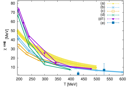
Figure 6: The fourth root of topological susceptibility versus the temperature for the full QCD studies reviewed here. This is only a subset of the results presented in the papers. (a) shows the gluonic results from Ref. [33]. (b) shows the tabulated results from Ref. [32]. (c) Ref. [135]: from these results we may infer the independence on the lattice spacing from the concordance between gluonic and fermionic methods; moreover we have rescaled the results with the pion mass. (d) and (d1) shows the results from Ref. [36], obtained by rescaling from the two lightest masses, $m_{\pi}=220$, 260 MeV. (e) the results from Ref. [136], where a careful continuum extrapolation with a conservative error estimate was performed.

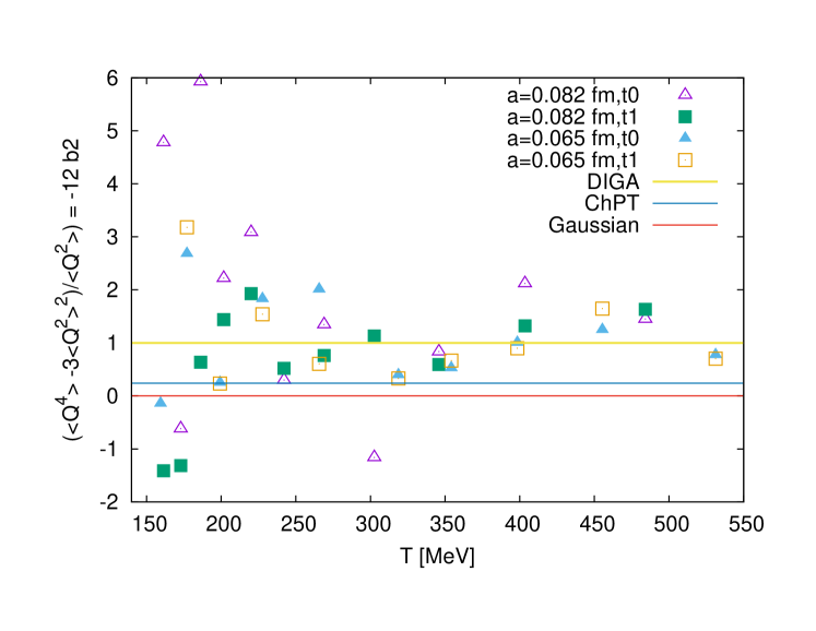
Figure 7: $b_{2}$ from lattice simulations with $N_{f}=2+1+1$ , and lattice spacings as indicated. $t_{0}$ and $t_{1}$ correspond to the two different levels of cooling. The gauge configurations are the same as in [36].

As we have briefly reviewed, all the authors contrast their power-law fits with the DIGA prediction, finding a reasonable agreement for $T\gtrsim 350$ MeV. To appreciate the approach to DIGA in some more detail, we present a summary in Figure 8, where we have considered the logarithmic derivative of the topological susceptibility [32, 36]. The log derivative[36] is rather noisy and the statistical errors overcome any mass/spacing systematics.

The average result confirms the approach to the DIGA limit above $T\sim 350$ MeV For Ref.[32] the log-derivative was computed using their tabulated results for the continuum topological susceptibility.

In comparison with the Yang-Mills results, the errors on the topological susceptibility are much larger. However, there are interesting common trends: at rather high temperatures, all the studies confirm a strong correction factor, despite the fact that the exponent is close to the DIGA prediction, a trend which was already observed in pure gauge.

Closer to $T_{c}$ we observe the largest spread in the results: perhaps it is not too surprising that a difficult observables feel the intricacy of the pseudocritical region – investigating and reaching a final conclusion on the behaviour of topology has bearing on the general properties of the transitions reviewed in Section 3.

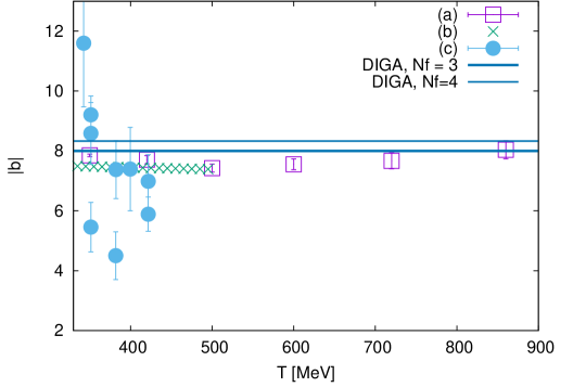
Figure 8: The absolute value of the exponent characterizing the power-law decay of the topological susceptibility at high temperatures: in the left hand side plot we show (a) log-derivative of the tabulated continuum results of $\chi_{top}$ [32]; (b) log-derivative of the continuum fit to the data of Ref. [33]; (c) log-derivative from the two lowest pion masses from the Wilson twisted study[36]. The results are contrasted with the DIGA limit prediction; in the right hand side plot the same results are summarized: for (a) we plot the results at $T=420,2100$ MeV, for (b) the average effective exponent in the temperature range considered; (c) shows the average and dispersion of the fit results for different pion masses in the temperature range $[200:600]$ MeV; (d) is result of the fit to the data of Ref.[135] in a restricted temperature range $T<350$ MeV.

6 The QCD Axion

We have mentioned that within the predicted bound $f_{A}\gtrsim 4\times 10^{8}$ the axion may contribute to contemporary density of cold dark matter. How this is realised, and the quantitative significance of the contribution, depends on the axion’s cosmological history [19, 141, 142]. Early studies using models[18, 143] identified the relevant temperature range $\mathcal{O}(1)$ GeV. A recent estimate of the temperatures of relevance is $500\lesssim T\lesssim 1500$ MeV [144]. To be useful for cosmology lattice simulations need to produce controlled results in this range.

In a nutshell, there are two main sources of axion production: by a thermal bath, producing hot axions, and by the so-called realignment mechanisms, which produces cold axions [15, 16, 17]. These cold axions are those that can provide observable dark matter. We will briefly review here how the typical parameters of axion’s evolution – in particular, the temperature dependence of the topological susceptibility – affect the final density of dark matter.

The cosmological history of the axion begins with the PQ symmetry breaking – at $T_{PQ}\simeq f_{A}$. At this point the axion field $a(x)$ will set somewhere at the bottom of the Mexican Hat, with an angle $\theta_{1}$ ”misaligned” with the conserving CP minimum $\theta=0$ of the contemporary potential. Axion is then a massless Goldstone boson. As time passes, temperature goes further down, and the dynamics becomes sensitive to the $U(1)$ breaking term (the topological fluctuations), i.e. to the axion potential $V(a)=\chi_{top}(T)(1-\cos(a/f_{A}))$. The axion is now a massive pseudo-Goldstone boson, ”oscillating” around the minimum.

The axion contribution to the cosmological density could be, in principle, estimated by solving the equation of motion for the axion field in spacetime. We give here a brief summing up of the main approximations, which have been used to arrive at a simple expression relating contemporary axion mass with the parameters characterizing the topological susceptibility evolution with temperature. In the following we will contrast the lattice data with the DIGA inspired behaviour, Eq. (10),

$$\chi_{top}=A\,T^{b}$$ (33)

and we will discuss the impact on the results for the bounds on the contemporary axion mass inferred from the variability of the parameters $A$ and $b$.

A few years ago[31] the first lattice studies aimed at extracting limits on the axion mass appeared, initially in the quenched limit, followed by simulations in full QCD[32, 59, 33, 35, 36]. In the previous Section we have reviewed the results for the topological susceptibility, and here we will discuss their impact on axion’s density and mass.

On general grounds, the results will depend on the initial angle $\theta_{1}$: if the PQ transition happened during, or before, the inflation, the initial angle $\theta_{1}$ will be made homogeneous in all the space-time. $\theta_{1}$ is arbitrary, the final predictions will depend on it, leading to large uncertainties. After inflation, contributions from different regions of space time will be averaged, and there will be no dependence on the initial angle. It is customary to refer to these two scenarios as pre-inflationary and post-inflationary, respectively.

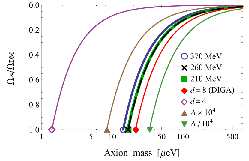
Figure 9: The axion contribution to Dark Matter versus the axion mass[36]: the first three lines show the results for three pion masses, $m_{\pi}=370$, 260, and 210 MeV, respectively, all rescaled to the physical pion mass according to $\chi_{top}\propto m_{\pi}^{4}$. The other lines are mock data meant to study the sensitivity on the errors to the fit parameters of the topological susceptibility $\chi_{top}\simeq A\,T^{-d}$, see text for discussions. Figure taken from Ref.[36].

The topological susceptibility enters the equation of motion for the axion degree of freedom $\theta$ via the potential $V(\theta)=\chi_{top}(\theta)f(\theta)\simeq\chi_{top}(\theta)(1-\cos\theta)$,

$$\ddot{\theta}+3H\dot{\theta}+V^{\prime}(\theta)=0,$$ (34)

where $H$ is the Hubble parameter[15, 18]. At early times the solution of Eq. (34) is a constant $\theta=\theta_{1}=\text{const}$. When the axion mass is of the order of the inverse of the Hubble parameter: $3H(T)=m_{A}(T)=\sqrt{\chi_{top}(T)}/f_{A}$, $\theta$ starts oscillating. The Hubble parameter can be approximated as

$$H(T)=\frac{\pi g_{*}^{1/2}(T)\,T^{2}}{\sqrt{90}\,M_{Pl}}.$$ (35)

$g_{*}(T)$ is the effective number of relativistic degrees of freedom, which has been computed up to $T=3$ GeV in the study reviewed above[32]. To obtain simple expressions in closed form we employ the power-law parameterization $g^{*}(T)=50.8\,(T/(\text{MeV}))^{0.053}$ reproducing the results[32] up to a few percents in the temperature interval $800<T<1500$ MeV.

The knowledge of the temperature dependence of the topological susceptibility determines the time of beginning of the oscillations as a function of $f_{A}$, or, equivalently, of $m_{A}$, if one trades $f_{A}$ for the zero temperature topological susceptibility and the axion mass via $\chi_{top}=f_{A}^{2}m_{A}^{2}$. Since then, time-averaged oscillations behave as pressureless dark matter [15], and the energy density $\rho_{A}(T)$ of the oscillating axion field is approximately the same as a collection of axions at rest: $\rho_{A}(T)\approx 1/2m_{A}^{2}(T)f_{A}^{2}\theta^{2}$. Hence the number density $n_{A}(T)=\rho_{A}(T)/m_{A}(T)$ can be estimated as $n_{A}(T)\approx 1/2m_{A}(T)f_{A}^{2}\theta^{2}$ .

The axion-to-entropy ratio remains constant after the beginning of the oscillations: knowing this ratio at the beginning of the oscillation, one can estimate the contribution of the axion to today’s density $\rho_{A,0}=\dfrac{n_{A}(T)}{s(T)}m_{A}s_{0}$, where $s$, $s_{0}$ are the entropies at time $T$, and of today, and $\Omega_{A}=\dfrac{\rho_{A,0}}{\rho_{c}}$, with $\rho_{c}$ the critical density.

In this simplified picture, the resulting axion density depends on the axion mass, on the topological susceptibility parameters $A,b$ and on $\theta_{1}$, the initial misalignment angle. For instance[36]:

$$\rho_{A}(m_{A})=\rho_{A}(m_{A},b,\theta_{1})=\rho_{A}(m_{A})=C(A,b,\theta_{1})m_{A}^{-\frac{3.053-b/2}{2.027-b/2}},$$ (36)

where we have highlighted the most relevant dependence on the exponent $b$. The coefficient $C$ depends on $b$ only weakly, and of course includes the relevant cosmological constants.

Note again the dependence on $\theta_{1}$: in a post-inflactionary scenario the misalignment angle can be averaged over. Anharmonicity effects on the potential may be included as well, but have little impact[31]. The pre-inflactionary scenario allows more freedom: clearly one can cover a wide range of axion masses by suitably adjusting the initial misalignment angle $\theta_{1}$[14].

Considering now the post-inflactionary scenario, the final density of axions can be contrasted with the known dark matter density to arrive at a bound on the contemporary axion mass[15, 16, 17]. However, one has to deal with a more complicated dynamics associated, essentially, with the possible presence of strings, domain walls and other forms of non-homogeneous structures such as archioles[14, 145, 146, 147, 148]. This limits the contribution to dark matter coming from axions alone, and it is a subject of contemporary research [133, 134]: even in the unlikely case that axion dynamics is the only responsible for dark matter, one cannot reach the overclosure bound with axion density alone.

In short, and simplifying, the amount of post-inflactionary axion dark matter can then be divided into a re-alignment contribution and a contribution from axionic strings and domain walls.

Consider now the contribution from re-alignment. The estimate [32] gives an absolute lower bound of $m_{A}=28(2)$ $\mu$eV, and $m_{A}=50(4)$ $\mu$eV if the contribution from misalignment mechanism contributes 50% to dark matter.

The study[33] combines lattice results and DIGA predictions and reports $f_{A}\leq 1.2(0.152)\times 10^{12}$ GeV, when this contribution matches the total amount of Dark Matter.

The results [36] are presented in a graphic form in Figure 9: the axion’s fractional contribution to Dark Matter is shown versus the axion mass for various situations. The first three lines are obtained from the results of three different pion masses, rescaled to the physical pion mass. The discrepancy between the results are very small at practical level. The impact of the uncertainties may be estimated by plotting a few mock curves, varying the parameters $A$ and $b$ using the central results as baseline. In all cases the intercept with the abscissa axis (overclosure bound) defines the absolute lower bound for the axion mass [36] $m_{A}\simeq 20(5)$ $\mu$eV, where the error is estimated from the spread of the results of the (plausible) fits. Clearly the bounds are robust against ’small’ changes of parameters. However, a significant variability remains, and, in particular, a slower decay would significantly lower the limit.

Even larger uncertainties come from the strings and domain wall contributions – recent estimates[21, 149], using as an input the results[32] for the topological susceptibility, conclude that the total axion dark matter, computed adding the contributions from strings and domain walls to the one from misalignment, fits the total amount of dark matter if $m_{A}>50$ $\mu$eV. Recent researches including an improved analysis of the string dynamics[145, 9, 150], give $m_{A}>(26.2\pm 3.4)$ $\mu$eV [145].

As for the pre-inflactionary scenario, the freedom of adjusting $\theta_{1}$ leads to a great variability for the axion density (see Eq. (34)), and the final result is less constrained, with values of the lower bound for the axion mass which may be reduced by two orders of magnitude.

Figure 10 summarizes the results for the acceptable range of axion masses emerging from these discussions.

The lower bounds on the post-inflactionary axion mass from the lattice calculations, in the case of QCD axions saturating all the Dark Matter, are marked as (a-d). In very short summary (a)[32] relies on a convincing continuum result, and on direct measurements in a broad range of temperatures; (b)[33] and (d)[36, 35] explored a more restricted temperature range, and relied on extrapolations, in addition (d) needed a rescaling to physical pion mass; (c)[34] suffers from lattice artifacts, which have been already to some extent clarified[136]. Finally, (e)[145] includes contributions from axion string dynamics, still using input from lattice results[32].

From Figure 9, and from similar results on the other works, one can see how an increasing axion mass would correspondingly lower the contribution to Dark Matter: indicatively, one places a tentative upper bound on the axion mass at $1500$ $\mu$eV, when the axion dark matter fraction is at the level of one percent.

Finally, in the pre-inflactionary situation, different choices for the initial misalignment angle basically would allow any value for the axion mass within the entire range spanned by $m_{A}$ in Figure 10.

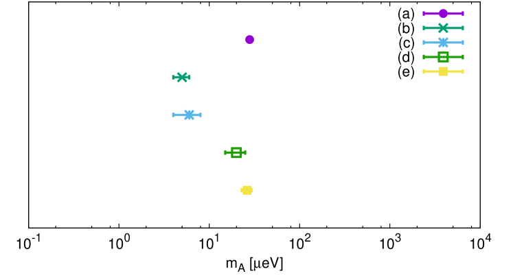
Figure 10: The results for the lower bound on the post-inflactionary axion mass discussed in the text. The results in (a)[32]; (b)[33] (c)[34] (d)[36] are the contributions from misalignment from lattice simulations; (e)[145] includes contributions from axion string dynamics. The $x$ axis approximatively spans the allowed range from cold axions: beyond the upper limit the contibution from axions would become negligeable. In the preinflactionary scenario the variability of the $\theta$ angle allows the smaller values of the axion mass corresponding to the lower limit set by astrophysical constraints.

Axion masses in the window discussed will be probed in the upcoming decade by direct detection experiments such as MADMAX, ADMX, CAPP, HAYSTAC, RADES, ORPHEUS and others. Recent reviews discuss these prospectives at different level of details[44, 41].

7 Parting remarks

Axions are well motivated candidates for Dark Matter, and QCD topology in the range $500\lesssim T\lesssim 1500$ MeV provides important input for the prediction of some of their properties. We have reviewed the current status of studies of topology in QCD, and we have discussed the implications on axion physics, in particular the limits on the post-inflactionary axion mass.

At zero temperature, QCD topology is a mature field, and the lattice results compare well with phenomenology and other estimates from model calculations. At very high temperature topology is constrained by instanton models. The vast range of temperatures in between is studied by ab-initio simulations of QCD on the lattice, which we have reviewed in this paper.

In the pure gauge theory, topology is becoming increasingly accurate: results from different approaches are in good agreement, within small residual errors.

The first results for topology in high temperature QCD are relatively recent. We have discussed the steady progress and the remaining uncertainties of the lattice calculations. For temperatures above 350 MeV topology faces in principle several technical problems, which we have reviewed. Nonetheless, a consistent picture emerges, indicating the approach to the DIGA limit for the temperature dependence of the susceptibility, and to the periodical form of the potential. A complete quantitative agreement among different lattice results has not been reached yet. There is however a substantial agreement on the possible sources of not-yet-quantified systematic errors, and improvements are within reach.

Accurate measurements of the topological susceptibility in QCD are important in order to quantify the mis-alignment contribution to axion dark matter. Beside mis-alignment, the current contribution of the axions to Dark Matter is affected by many sources of uncertainty, including those coming from topological defects which necessarily accompany the production of post-inflactionary axions. Lattice results are also used as input to the analysis of these contributions.

The bounds on the axion mass derived from lattice results point at a range which is well within the reach of current experiments. The lattice studies predict a lower bound on the post-inflactionary axion mass from mis-alignment ranging from $m_{A}\simeq 5$ $\mu$eV till $m_{A}\simeq 28$ $\mu$eV, assuming that all Dark Matter is made of axions. The sensitivity of the axion mass to the fraction of Dark Matter contributed by the mis-alignment mechanism can be read off Figure 9. The analysis of the contribution from strings, which still relies on lattice results, gives a lower bound $m_{A}=(26.2\pm 3.4)$ $\mu$eV. Further effects are under active investigation.

One final comment concerns the region around the QCD phase transition, where the interrelation of topology, chiral and axial symmetry has a profound influence. The general picture there is not completely understood, and constitutes a main focus of the current research in the physics of strong interactions.

References

- [1] R. Peccei and H. R. Quinn, Phys. Rev. Lett. 38, 1440 (1977), 10.1103/PhysRevLett.38.1440.
- [2] R. Peccei and H. R. Quinn, Phys. Rev. D 16, 1791 (1977), 10.1103/PhysRevD.16.1791.
- [3] S. Weinberg, Phys. Rev. Lett. 40, 223 (1978), 10.1103/PhysRevLett.40.223.
- [4] F. Wilczek, Phys. Rev. Lett. 40, 279 (1978), 10.1103/PhysRevLett.40.279.
- [5] G. ’t Hooft, Phys. Rev. Lett. 37, 8 (1976), 10.1103/PhysRevLett.37.8.
- [6] G. ’t Hooft, Phys. Rev. D 14, 3432 (1976), 10.1103/PhysRevD.14.3432, [Erratum: Phys.Rev.D 18, 2199 (1978)].
- [7] S. Weinberg, Phys. Rev. D 11, 3583 (1975), 10.1103/PhysRevD.11.3583.
- [8] G. Grilli di Cortona, E. Hardy, J. Pardo Vega and G. Villadoro, JHEP 01, 034 (2016), arXiv:1511.02867 [hep-ph], 10.1007/JHEP01(2016)034.
- [9] M. Gorghetto and G. Villadoro, JHEP 03, 033 (2019), arXiv:1812.01008 [hep-ph], 10.1007/JHEP03(2019)033.
- [10] R. Mayle, J. R. Wilson, J. R. Ellis, K. A. Olive, D. N. Schramm and G. Steigman, Phys. Lett. B 203, 188 (1988), 10.1016/0370-2693(88)91595-X.
- [11] G. G. Raffelt, Lect. Notes Phys. 741, 51 (2008), arXiv:hep-ph/0611350, 10.1007/978-3-540-73518-2_3.
- [12] M. I. Vysotsky, Ya. B. Zeldovich, M. Yu. Khlopov and V. M. Chechetkin, Pisma Zh. Eksp. Teor. Fiz. 27, 533 (1978), [JETP Lett.27,502(1978)].
- [13] E. Braaten and H. Zhang, Rev. Mod. Phys. 91, 041002 (2019), 10.1103/RevModPhys.91.041002.
- [14] A. Ringwald, Axion mass in the case of post-inflationary Peccei-Quinn symmetry breaking (5 2018). arXiv:1805.09618 [hep-ph].
- [15] J. Preskill, M. B. Wise and F. Wilczek, Phys. Lett. B 120, 127 (1983), 10.1016/0370-2693(83)90637-8.
- [16] L. Abbott and P. Sikivie, Phys. Lett. B 120, 133 (1983), 10.1016/0370-2693(83)90638-X.
- [17] M. Dine and W. Fischler, Phys. Lett. B 120, 137 (1983), 10.1016/0370-2693(83)90639-1.
- [18] O. Wantz and E. Shellard, Phys. Rev. D 82, 123508 (2010), arXiv:0910.1066 [astro-ph.CO], 10.1103/PhysRevD.82.123508.
- [19] D. J. E. Marsh, Phys. Rept. 643, 1 (2016), arXiv:1510.07633 [astro-ph.CO], 10.1016/j.physrep.2016.06.005.
- [20] V. Rubakov, Cosmology and Dark Matter, in 2019 European School of High-Energy Physics, (12 2019). arXiv:1912.04727 [hep-ph].
- [21] G. Ballesteros, J. Redondo, A. Ringwald and C. Tamarit, Front. Astron. Space Sci. 6, 55 (2019), arXiv:1904.05594 [hep-ph], 10.3389/fspas.2019.00055.
- [22] D. J. Gross, R. D. Pisarski and L. G. Yaffe, Rev. Mod. Phys. 53, 43 (1981), 10.1103/RevModPhys.53.43.
- [23] A. Ringwald and F. Schrempp, Phys. Lett. B 459, 249 (1999), arXiv:hep-lat/9903039, 10.1016/S0370-2693(99)00682-6.
- [24] S. Bottaro and E. Meggiolaro (4 2020), arXiv:2004.11901 [hep-ph].
- [25] H. Ding et al., Phys. Rev. Lett. 123, 062002 (2019), arXiv:1903.04801 [hep-lat], 10.1103/PhysRevLett.123.062002.
- [26] M. D’Elia, Nucl. Phys. A 982, 99 (2019), arXiv:1809.10660 [hep-lat], 10.1016/j.nuclphysa.2018.10.042.
- [27] O. Philipsen, Constraining the QCD phase diagram at finite temperature and density, in 37th International Symposium on Lattice Field Theory, (12 2019). arXiv:1912.04827 [hep-lat].
- [28] H.-T. Ding, New developments in lattice QCD on equilibrium physics and phase diagram, in 28th International Conference on Ultrarelativistic Nucleus-Nucleus Collisions, (2 2020). arXiv:2002.11957 [hep-lat].
- [29] M. Müller-Preussker, PoS LATTICE2014, 003 (2015), arXiv:1503.01254 [hep-lat], 10.22323/1.214.0003.
- [30] C. Bonati, EPJ Web Conf. 175, 01011 (2018), arXiv:1710.06410 [hep-lat], 10.1051/epjconf/201817501011.
- [31] E. Berkowitz, M. I. Buchoff and E. Rinaldi, Phys. Rev. D 92, 034507 (2015), arXiv:1505.07455 [hep-ph], 10.1103/PhysRevD.92.034507.
- [32] S. Borsanyi et al., Nature 539, 69 (2016), arXiv:1606.07494 [hep-lat], 10.1038/nature20115.
- [33] P. Petreczky, H.-P. Schadler and S. Sharma, Phys. Lett. B 762, 498 (2016), arXiv:1606.03145 [hep-lat], 10.1016/j.physletb.2016.09.063.
- [34] C. Bonati, M. D’Elia, M. Mariti, G. Martinelli, M. Mesiti, F. Negro, F. Sanfilippo and G. Villadoro, JHEP 03, 155 (2016), arXiv:1512.06746 [hep-lat], 10.1007/JHEP03(2016)155.
- [35] F. Burger, E.-M. Ilgenfritz, M. P. Lombardo, M. Müller-Preussker and A. Trunin, Nucl. Phys. A 967, 880 (2017), arXiv:1705.01847 [hep-lat], 10.1016/j.nuclphysa.2017.07.006.
- [36] F. Burger, E.-M. Ilgenfritz, M. P. Lombardo and A. Trunin, Phys. Rev. D 98, 094501 (2018), arXiv:1805.06001 [hep-lat], 10.1103/PhysRevD.98.094501.
- [37] P. Svrcek and E. Witten, JHEP 06, 051 (2006), arXiv:hep-th/0605206, 10.1088/1126-6708/2006/06/051.
- [38] P. Anastasopoulos, P. Betzios, M. Bianchi, D. Consoli and E. Kiritsis, JHEP 19, 113 (2020), arXiv:1811.05940 [hep-ph], 10.1007/JHEP10(2019)113.
- [39] F. Bigazzi, A. Caddeo, A. L. Cotrone, P. Di Vecchia and A. Marzolla, JHEP 12, 056 (2019), arXiv:1906.12117 [hep-th], 10.1007/JHEP12(2019)056.
- [40] P. Di Vecchia, M. Giannotti, M. Lattanzi and A. Lindner, PoS Confinement2018, 034 (2019), arXiv:1902.06567 [hep-ph], 10.22323/1.336.0034.
- [41] I. G. Irastorza and J. Redondo, Prog. Part. Nucl. Phys. 102, 89 (2018), arXiv:1801.08127 [hep-ph], 10.1016/j.ppnp.2018.05.003.
- [42] P. Sikivie (3 2020), arXiv:2003.02206 [hep-ph].
- [43] L. Di Luzio, M. Giannotti, E. Nardi and L. Visinelli (3 2020), arXiv:2003.01100 [hep-ph].
- [44] J. Jaeckel, M. Lamont and C. Vallée, Nature Phys. 16, 393 (2020), 10.1038/s41567-020-0838-4.
- [45] M. Pospelov and A. Ritz, Nucl. Phys. B 573, 177 (2000), arXiv:hep-ph/9908508, 10.1016/S0550-3213(99)00817-2.
- [46] A. Pich and E. de Rafael, Nucl. Phys. B 367, 313 (1991), 10.1016/0550-3213(91)90019-T.
- [47] nEDM Collaboration (C. Abel et al.), Phys. Rev. Lett. 124, 081803 (2020), arXiv:2001.11966 [hep-ex], 10.1103/PhysRevLett.124.081803.
- [48] E. Vicari and H. Panagopoulos, Phys. Rept. 470, 93 (2009), arXiv:0803.1593 [hep-th], 10.1016/j.physrep.2008.10.001.
- [49] J. E. Kim, Phys. Rept. 150, 1 (1987), 10.1016/0370-1573(87)90017-2.
- [50] P. Di Vecchia and G. Veneziano, Nucl. Phys. B 171, 253 (1980), 10.1016/0550-3213(80)90370-3.
- [51] C. Rosenzweig, J. Schechter and C. Trahern, Phys. Rev. D 21, 3388 (1980), 10.1103/PhysRevD.21.3388.
- [52] A. Gómez Nicola, J. Ruiz De Elvira and A. Vioque-Rodríguez, JHEP 11, 086 (2019), arXiv:1907.11734 [hep-ph], 10.1007/JHEP11(2019)086.
- [53] B.-J. Schaefer and M. Mitter, Acta Phys. Polon. Supp. 7, 81 (2014), arXiv:1312.3850 [hep-ph], 10.5506/APhysPolBSupp.7.81.
- [54] G. Veneziano, Nucl. Phys. B 159, 213 (1979), 10.1016/0550-3213(79)90332-8.
- [55] R. N. Larsen, S. Sharma and E. Shuryak (12 2019), arXiv:1912.09141 [hep-lat].
- [56] R. N. Larsen, S. Sharma and E. Shuryak, Phys. Lett. B 794, 14 (2019), arXiv:1811.07914 [hep-lat], 10.1016/j.physletb.2019.05.019.
- [57] S. Sharma, PoS LATTICE2018, 009 (2019), arXiv:1901.07190 [hep-lat], 10.22323/1.334.0009.
- [58] P. Di Vecchia, G. Rossi, G. Veneziano and S. Yankielowicz, JHEP 12, 104 (2017), arXiv:1709.00731 [hep-th], 10.1007/JHEP12(2017)104.
- [59] C. Bonati, M. D’Elia, P. Rossi and E. Vicari, Phys. Rev. D 94, 085017 (2016), arXiv:1607.06360 [hep-lat], 10.1103/PhysRevD.94.085017.
- [60] M. Dine, TASI lectures on the strong CP problem, in Flavor physics for the millennium. Proceedings, Theoretical Advanced Study Institute in elementary particle physics, TASI 2000, Boulder, USA, June 4-30, 2000, (6 2000), pp. 349–369. arXiv:hep-ph/0011376.
- [61] E. Witten, Nucl. Phys. B156, 269 (1979), 10.1016/0550-3213(79)90031-2.
- [62] T. Feldmann, Int. J. Mod. Phys. A15, 159 (2000), arXiv:hep-ph/9907491 [hep-ph], 10.1142/S0217751X00000082.
- [63] L. Del Debbio, L. Giusti and C. Pica, Phys. Rev. Lett. 94, 032003 (2005), arXiv:hep-th/0407052 [hep-th], 10.1103/PhysRevLett.94.032003.
- [64] S. Durr, Z. Fodor, C. Hoelbling and T. Kurth, JHEP 04, 055 (2007), arXiv:hep-lat/0612021 [hep-lat], 10.1088/1126-6708/2007/04/055.
- [65] ETM Collaboration (K. Cichy, E. Garcia-Ramos, K. Jansen, K. Ottnad and C. Urbach), JHEP 09, 020 (2015), arXiv:1504.07954 [hep-lat], 10.1007/JHEP09(2015)020.
- [66] D. Horvatić, D. Kekez and D. Klabuˇcar, Phys. Rev. D 99, 014007 (2019), arXiv:1809.00379 [hep-ph], 10.1103/PhysRevD.99.014007.
- [67] J. I. Kapusta, E. Rrapaj and S. Rudaz, Phys. Rev. C 101, 031901 (2020), arXiv:1910.12759 [nucl-th], 10.1103/PhysRevC.101.031901.
- [68] J. I. Kapusta, D. Kharzeev and L. D. McLerran, Phys. Rev. D 53, 5028 (1996), arXiv:hep-ph/9507343, 10.1103/PhysRevD.53.5028.
- [69] E. V. Shuryak, Comments Nucl. Part. Phys. 21, 235 (1994), arXiv:hep-ph/9310253.
- [70] S. Resch, F. Rennecke and B.-J. Schaefer, Phys. Rev. D 99, 076005 (2019), arXiv:1712.07961 [hep-ph], 10.1103/PhysRevD.99.076005.
- [71] F. Gao and J. M. Pawlowski (2 2020), arXiv:2002.07500 [hep-ph].
- [72] L. Mazur, O. Kaczmarek, E. Laermann and S. Sharma, PoS LATTICE2018, 153 (2019), arXiv:1811.08222 [hep-lat], 10.22323/1.334.0153.
- [73] HotQCD Collaboration, S. Sharma, The fate of and topological features of QCD at finite temperature, in 11th International Workshop on Critical Point and Onset of Deconfinement, (1 2018). arXiv:1801.08500 [hep-lat].
- [74] JLQCD Collaboration (H. Fukaya), EPJ Web Conf. 175, 01012 (2018), arXiv:1712.05536 [hep-lat], 10.1051/epjconf/201817501012.
- [75] HotQCD Collaboration (S. Sharma), PoS CPOD2017, 086 (2018), 10.22323/1.311.0086.
- [76] C. Schmidt and S. Sharma, J. Phys. G 44, 104002 (2017), arXiv:1701.04707 [hep-lat], 10.1088/1361-6471/aa824a.
- [77] A. Tomiya, G. Cossu, S. Aoki, H. Fukaya, S. Hashimoto, T. Kaneko and J. Noaki, Phys. Rev. D 96, 034509 (2017), arXiv:1612.01908 [hep-lat], 10.1103/PhysRevD.96.034509, [Addendum: Phys.Rev.D 96, 079902 (2017)].
- [78] A. Y. Kotov, M. P. Lombardo and A. M. Trunin, Phys. Lett. B 794, 83 (2019), arXiv:1903.05633 [hep-lat], 10.1016/j.physletb.2019.05.035.
- [79] A. Y. Kotov, M. P. Lombardo and A. M. Trunin (4 2020), arXiv:2004.07122 [hep-lat].
- [80] R. D. Pisarski and F. Wilczek, Phys. Rev. D 29, 338 (1984), 10.1103/PhysRevD.29.338.
- [81] A. Pelissetto and E. Vicari, Phys. Rev. D 88, 105018 (2013), arXiv:1309.5446 [hep-lat], 10.1103/PhysRevD.88.105018.
- [82] tmfT Collaboration (F. Burger, E.-M. Ilgenfritz, M. Kirchner, M. P. Lombardo, M. Müller-Preussker, O. Philipsen, C. Urbach and L. Zeidlewicz), Phys. Rev. D 87, 074508 (2013), arXiv:1102.4530 [hep-lat], 10.1103/PhysRevD.87.074508.
- [83] G. Aarts et al., Spectral quantities in thermal QCD: a progress report from the FASTSUM collaboration, in 37th International Symposium on Lattice Field Theory, (2019). arXiv:1912.09827 [hep-lat].
- [84] LLNL/RBC Collaboration Collaboration (M. I. Buchoff, M. Cheng, N. H. Christ, H.-T. Ding, C. Jung, F. Karsch, Z. Lin, R. D. Mawhinney, S. Mukherjee, P. Petreczky, D. Renfrew, C. Schroeder, P. M. Vranas and H. Yin), Phys. Rev. D 89, 054514 (Mar 2014), arXiv:1309.4149 [hep-lat], 10.1103/PhysRevD.89.054514.
- [85] T. D. Cohen, Phys. Rev. D 54, 1867 (1996), arXiv:hep-ph/9601216, 10.1103/PhysRevD.54.R1867.
- [86] O. Kaczmarek, F. Karsch, A. Lahiri, L. Mazur and C. Schmidt, QCD phase transition in the chiral limit (3 2020). arXiv:2003.07920 [hep-lat].
- [87] JLQCD Collaboration, K. Suzuki, S. Aoki, Y. Aoki, G. Cossu, H. Fukaya, S. Hashimoto and C. Rohrhofer, Axial U(1) symmetry and mesonic correlators at high temperature in lattice QCD, in 37th International Symposium on Lattice Field Theory, (1 2020). arXiv:2001.07962 [hep-lat].
- [88] T. Kanazawa and N. Yamamoto, JHEP 01, 141 (2016), arXiv:1508.02416 [hep-th], 10.1007/JHEP01(2016)141.
- [89] S. Aoki, H. Fukaya and Y. Taniguchi, Phys. Rev. D 86, 114512 (2012), arXiv:1209.2061 [hep-lat], 10.1103/PhysRevD.86.114512.
- [90] B. B. Brandt, M. Cè, A. Francis, T. Harris, H. B. Meyer, H. Wittig and O. Philipsen, PoS CD2018, 055 (2019), arXiv:1904.02384 [hep-lat], 10.22323/1.317.0055.
- [91] B. B. Brandt, A. Francis, H. B. Meyer, O. Philipsen, D. Robaina and H. Wittig, JHEP 12, 158 (2016), arXiv:1608.06882 [hep-lat], 10.1007/JHEP12(2016)158.
- [92] G. Cossu, S. Aoki, H. Fukaya, S. Hashimoto, T. Kaneko, H. Matsufuru and J.-I. Noaki, Phys. Rev. D 87, 114514 (2013), arXiv:1304.6145 [hep-lat], 10.1103/PhysRevD.87.114514, [Erratum: Phys.Rev.D 88, 019901 (2013)].
- [93] TWQCD Collaboration (T.-W. Chiu, W.-P. Chen, Y.-C. Chen, H.-Y. Chou and T.-H. Hsieh), PoS LATTICE2013, 165 (2014), arXiv:1311.6220 [hep-lat], 10.22323/1.187.0165.
- [94] J. Braun, W.-J. Fu, J. M. Pawlowski, F. Rennecke, D. Rosenblüh and S. Yin (3 2020), arXiv:2003.13112 [hep-ph].
- [95] T. Bhattacharya et al., Phys. Rev. Lett. 113, 082001 (2014), arXiv:1402.5175 [hep-lat], 10.1103/PhysRevLett.113.082001.
- [96] HotQCD Collaboration (A. Bazavov et al.), Phys. Lett. B795, 15 (2019), arXiv:1812.08235 [hep-lat], 10.1016/j.physletb.2019.05.013.
- [97] C. Alexandrou et al., Phys. Rev. D98, 054518 (2018), arXiv:1807.00495 [hep-lat], 10.1103/PhysRevD.98.054518.
- [98] H. J. Rothe, World Sci. Lect. Notes Phys. 43, 1 (1992), [World Sci. Lect. Notes Phys.59,1(1997); World Sci. Lect. Notes Phys.74,1(2005); World Sci. Lect. Notes Phys.82,1(2012)].
- [99] I. Montvay and G. Munster, Quantum fields on a latticeCambridge Monographs on Mathematical Physics, Cambridge Monographs on Mathematical Physics (Cambridge University Press, 1997).
- [100] T. DeGrand and C. E. Detar, Lattice methods for quantum chromodynamics 2006.
- [101] C. Gattringer and C. B. Lang, Lect. Notes Phys. 788, 1 (2010), 10.1007/978-3-642-01850-3.
- [102] L. Lellouch, R. Sommer, B. Svetitsky, A. Vladikas and L. F. Cugliandolo (eds.), Modern perspectives in lattice QCD: Quantum field theory and high performance computing. Proceedings, International School, 93rd Session, Les Houches, France, August 3-28, 2009, 2011).
- [103] R. W. Jackiw, Scholarpedia 3, 7302 (2008), 10.4249/scholarpedia.7302.
- [104] S. O. Bilson-Thompson, F. D. R. Bonnet, D. B. Leinweber and A. G. Williams, Nucl. Phys. Proc. Suppl. 109A, 116 (2002), arXiv:hep-lat/0112034 [hep-lat], 10.1016/S0920-5632(02)01399-3.
- [105] S. O. Bilson-Thompson, D. B. Leinweber and A. G. Williams, Annals Phys. 304, 1 (2003), arXiv:hep-lat/0203008 [hep-lat], 10.1016/S0003-4916(03)00009-5.
- [106] A. Hasenfratz and F. Knechtli, Phys. Rev. D64, 034504 (2001), arXiv:hep-lat/0103029 [hep-lat], 10.1103/PhysRevD.64.034504.
- [107] C. Morningstar and M. J. Peardon, Phys. Rev. D69, 054501 (2004), arXiv:hep-lat/0311018 [hep-lat], 10.1103/PhysRevD.69.054501.
- [108] P. J. Moran and D. B. Leinweber, Phys. Rev. D77, 094501 (2008), arXiv:0801.1165 [hep-lat], 10.1103/PhysRevD.77.094501.
- [109] M. Luscher, JHEP 08, 071 (2010), arXiv:1006.4518 [hep-lat], 10.1007/JHEP08(2010)071, 10.1007/JHEP03(2014)092, [Erratum: JHEP03,092(2014)].
- [110] M. Luscher and P. Weisz, JHEP 02, 051 (2011), arXiv:1101.0963 [hep-th], 10.1007/JHEP02(2011)051.
- [111] C. Bonati and M. D’Elia, Phys. Rev. D89, 105005 (2014), arXiv:1401.2441 [hep-lat], 10.1103/PhysRevD.89.105005.
- [112] C. Alexandrou, A. Athenodorou and K. Jansen, Phys. Rev. D92, 125014 (2015), arXiv:1509.04259 [hep-lat], 10.1103/PhysRevD.92.125014.
- [113] C. Alexandrou, A. Athenodorou, K. Cichy, A. Dromard, E. Garcia-Ramos, K. Jansen, U. Wenger and F. Zimmermann (2017), arXiv:1708.00696 [hep-lat].
- [114] Y. Namekawa, PoS LATTICE2014, 344 (2015), arXiv:1501.06295 [hep-lat], 10.22323/1.214.0344.
- [115] K. Cichy, A. Dromard, E. Garcia-Ramos, K. Ottnad, C. Urbach, M. Wagner, U. Wenger and F. Zimmermann, PoS LATTICE2014, 075 (2014), arXiv:1411.1205 [hep-lat], 10.22323/1.214.0075.
- [116] A. Trunin, F. Burger, E.-M. Ilgenfritz, M. P. Lombardo and M. Müller-Preussker, J. Phys. Conf. Ser. 668, 012123 (2016), arXiv:1510.02265 [hep-lat], 10.1088/1742-6596/668/1/012123.
- [117] M. F. Atiyah and I. M. Singer, Annals Math. 93, 139 (1971), 10.2307/1970757.
- [118] M. F. Atiyah and I. M. Singer, Proc. Nat. Acad. Sci. 81, 2597 (1984), 10.1073/pnas.81.8.2597.
- [119] M. Luscher, Phys. Lett. B428, 342 (1998), arXiv:hep-lat/9802011 [hep-lat], 10.1016/S0370-2693(98)00423-7.
- [120] H. Neuberger, Phys. Lett. B417, 141 (1998), arXiv:hep-lat/9707022 [hep-lat], 10.1016/S0370-2693(97)01368-3.
- [121] H. Neuberger, Phys. Lett. B427, 353 (1998), arXiv:hep-lat/9801031 [hep-lat], 10.1016/S0370-2693(98)00355-4.
- [122] R. G. Edwards, U. M. Heller and R. Narayanan, Nucl. Phys. B535, 403 (1998), arXiv:hep-lat/9802016 [hep-lat], 10.1016/S0550-3213(98)00588-4.
- [123] L. Giusti and M. Luscher, JHEP 03, 013 (2009), arXiv:0812.3638 [hep-lat], 10.1088/1126-6708/2009/03/013.
- [124] M. Luscher and F. Palombi, JHEP 09, 110 (2010), arXiv:1008.0732 [hep-lat], 10.1007/JHEP09(2010)110.
- [125] J. B. Kogut, J. F. Lagae and D. K. Sinclair, Phys. Rev. D58, 054504 (1998), arXiv:hep-lat/9801020 [hep-lat], 10.1103/PhysRevD.58.054504.
- [126] HotQCD Collaboration (A. Bazavov et al.), Phys. Rev. D86, 094503 (2012), arXiv:1205.3535 [hep-lat], 10.1103/PhysRevD.86.094503.
- [127] C. Alexandrou, A. Athenodorou, K. Cichy, M. Constantinou, D. P. Horkel, K. Jansen, G. Koutsou and C. Larkin, Phys. Rev. D97, 074503 (2018), arXiv:1709.06596 [hep-lat], 10.1103/PhysRevD.97.074503.
- [128] R. Larsen, S. Sharma and E. Shuryak, PoS LATTICE2018, 156 (2018), 10.22323/1.334.0156.
- [129] B. Alles, M. D’Elia and A. Di Giacomo, Nucl. Phys. B 494, 281 (1997), arXiv:hep-lat/9605013, 10.1016/S0550-3213(97)00205-8, [Erratum: Nucl.Phys.B 679, 397–399 (2004)].
- [130] C. Gattringer, R. Hoffmann and S. Schaefer, Phys. Lett. B 535, 358 (2002), arXiv:hep-lat/0203013, 10.1016/S0370-2693(02)01757-4.
- [131] S. Borsanyi, M. Dierigl, Z. Fodor, S. D. Katz, S. W. Mages, D. Nogradi, J. Redondo, A. Ringwald and K. K. Szabo, Phys. Lett. B752, 175 (2016), arXiv:1508.06917 [hep-lat], 10.1016/j.physletb.2015.11.020.
- [132] L. Giusti and M. Lüscher, Eur. Phys. J. C 79, 207 (2019), arXiv:1812.02062 [hep-lat], 10.1140/epjc/s10052-019-6706-7.
- [133] P. T. Jahn, G. D. Moore and D. Robaina (2 2020), arXiv:2002.01153 [hep-lat].
- [134] P. T. Jahn, G. D. Moore and D. Robaina, PoS LATTICE2018, 155 (2018), arXiv:1810.13218 [hep-lat], 10.22323/1.334.0155.
- [135] Y. Taniguchi, K. Kanaya, H. Suzuki and T. Umeda, Phys. Rev. D 95, 054502 (2017), arXiv:1611.02411 [hep-lat], 10.1103/PhysRevD.95.054502.
- [136] C. Bonati, M. D’Elia, G. Martinelli, F. Negro, F. Sanfilippo and A. Todaro, JHEP 11, 170 (2018), arXiv:1807.07954 [hep-lat], 10.1007/JHEP11(2018)170.
- [137] M. Laine and A. Vuorinen, Basics of Thermal Field Theory (Springer, 2016).
- [138] M. Laine and Y. Schroder, Phys. Rev. D 73, 085009 (2006), arXiv:hep-ph/0603048, 10.1103/PhysRevD.73.085009.
- [139] S. Borsanyi, G. Endrodi, Z. Fodor, S. Katz and K. Szabo, JHEP 07, 056 (2012), arXiv:1204.6184 [hep-lat], 10.1007/JHEP07(2012)056.
- [140] F. Burger, E.-M. Ilgenfritz, M.P. Lombardo and A. Trunin, Axions and Topology in QCD, talk at ECT* workshop, October 2018.
- [141] P. Sikivie, Lect. Notes Phys. 741, 19 (2008), arXiv:astro-ph/0610440, 10.1007/978-3-540-73518-2_2.
- [142] A. Ringwald, Phys. Dark Univ. 1, 116 (2012), arXiv:1210.5081 [hep-ph], 10.1016/j.dark.2012.10.008.
- [143] M. S. Turner, Phys. Rev. D 33, 889 (1986), 10.1103/PhysRevD.33.889.
- [144] G. D. Moore, EPJ Web Conf. 175, 01009 (2018), arXiv:1709.09466 [hep-ph], 10.1051/epjconf/201817501009.
- [145] V. B. Klaer and G. D. Moore, JCAP 11, 049 (2017), arXiv:1708.07521 [hep-ph], 10.1088/1475-7516/2017/11/049.
- [146] A. Saurabh, T. Vachaspati and L. Pogosian, Phys. Rev. D 101, 083522 (2020), arXiv:2001.01030 [hep-ph], 10.1103/PhysRevD.101.083522.
- [147] A. S. Sakharov and M. Yu. Khlopov, Phys. Atom. Nucl. 57, 485 (1994), [Yad. Fiz.57,514(1994)].
- [148] A. S. Sakharov, D. D. Sokoloff and M. Yu. Khlopov, Phys. Atom. Nucl. 59, 1005 (1996), [Yad. Fiz.59N6,1050(1996)].
- [149] G. Ballesteros, J. Redondo, A. Ringwald and C. Tamarit, JCAP 08, 001 (2017), arXiv:1610.01639 [hep-ph], 10.1088/1475-7516/2017/08/001.
- [150] V. B. Klaer and G. D. Moore (12 2019), arXiv:1912.08058 [hep-ph].