On the complex singularities of the inverse Langevin function

Abstract

We study the inverse Langevin function $\mathscr{L}^{-1}(x)$ because of its importance in modelling limited-stretch elasticity where the stress and strain energy become infinite as a certain maximum strain is approached, modelled here by $x\to 1$. The only real singularities of the inverse Langevin function $\mathscr{L}^{-1}(x)$ are two simple poles at $x=\pm 1$ and we see how to remove their effects either multiplicatively or additively. In addition, we find that $\mathscr{L}^{-1}(x)$ has an infinity of complex singularities. Examination of the Taylor series about the origin of $\mathscr{L}^{-1}(x)$ shows that the four complex singularities nearest the origin are equidistant from the origin and have the same strength; we develop a new algorithm for finding these four complex singularities. Graphical illustration seems to point to these complex singularities being of a square root nature. An exact analysis then proves these are square root branch points.

Keywords Inverse Langevin function, limited-stretch rubber elasticity, polymer chains, square root singularities, branch points

[Received on 1 March 2018; revised on 22 August 2018; accepted on 24 August 2018]

1 Introduction

In modelling the stress softening of rubber or rubber-like materials many authors in the past have utilized either the James & Guth [13] three-chain model, the Wang & Guth [26] four-chain model, the Arruda & Boyce [1] eight-chain model or the Wu & Van der Giessen [27] full network model. Zúñiga & Beatty [28] and Beatty [2] give descriptions of these models, all of which are closely related to the original Kuhn & Grün [17] single-chain model. The chains referred to here are arbitrarily orientated chains of connected molecules. When these polymer chains are stretched to their maximum extent there results a maximum stretch of the rubber sample in the direction of extension. The stress response and strain energy then become infinite as this maximum stretch is reached. Such a model of rubber elasticity is said to be a limited-stretch elastic model.

The Langevin function is defined by

$$x=\mathscr{L}(y)=\coth y-1/y$$ (1.1)

which has a removable singularity at $y=0$ and is defined on the domain $-\infty<y<\infty$. All the above models, however, involve the inverse Langevin function defined by

$$y=\mathscr{L}^{-1}(x)$$ (1.2)

defined on the domain $-1<x<1$ with range $-\infty<y<\infty$. These are both odd functions though on physical grounds $y$ and $x$ may be restricted to be positive. It is the property $\mathscr{L}^{-1}(x)\to\infty$ as $x\to 1$ that makes the inverse Langevin function so useful in modelling limited-stretch elasticity.

The Arruda & Boyce [1] eight-chain model has proved to be the most successful of these models, both theoretically and experimentally. However, Beatty [2] has shown that quite remarkably the Arruda & Boyce [1] stress response holds in general in isotropic nonlinear elasticity for a full network model of arbitrarily orientated molecular chains. Thus the eight-chain cell structure is unnecessary and so the inverse Langevin function has an important role to play in the theory of the finite isotropic elasticity of rubber and rubber-like materials.

The inverse Langevin function cannot be expressed in closed form and so many approximations to it have been devised and applied to many models of rubber elasticity. Perhaps the simplest is to consider the Taylor series but this does not converge over the whole domain of definition $-1<x<1$ of the inverse Langevin function, see [12] and [11]. Cohen [4] derived an approximation based upon a $[3/2]$ Padé approximant of the inverse Langevin function which has been widely used and is fairly accurate over the whole domain of definition. Many more accurate approximations have been devised, see for example, [5, 14, 15, 16, 18, 20, 21, 23, 24]. However, rather than finding further approximations to the inverse Langevin function, we emphasise in this paper how to find the approximate positions of its singularities in the complex plane. We are also able to find exactly the positions and nature of these singularities.

This paper is structured as follows. In Section 2 we give a brief account of non-linear isotropic elasticity theory as applied to the limited-stretch theory of elasticity of, for example, [1] and [2]. In Section 3 we define and discuss the Langevin and inverse Langevin functions, giving Taylor series for both, and identify the real singularities of the inverse Langevin function to be two simple poles. We see that the effects of these poles may be removed either multiplicatively or additively. In Section 4 we give approximate methods for analysing the Taylor series of functions with four complex singularities equidistant from the origin. First, in Section 4.1 we extend the methods of Mercer & Roberts [19] and Hunter & Guerrieri [10] in the two-singularity case to the present situation of four complex singularities equidistant from the origin and develop an algorithm for estimating the four complex singularities with the smallest radius of convergence. Then, in Section 4.2 a continued fraction method is used to calculate the poles and zeros of the Taylor series approximation and also the method of Padé approximants is considered. In Section 5.1 there is a graphical representation of the four branch cut singularities nearest the origin found using the methods developed in subsection 4.1. In Section 5.2 these methods are used to discuss and illustrate the branch cut singularities which are the next-nearest to the origin and in Section 5.3 there is a brief discussion of Euler’s method for removing the four nearest singularities to infinity. An exact analysis of the complex singularities of the inverse Langevin function is given in Section 6. The complex singularities are identified as square root branch points and the first 100 are given in Tables 3 and 4 correct to 15 significant figures. Finally, a discussion of the results is given in Section 7.

2 Non-linear isotropic incompressible elasticity for rubber-like materials and polymers

The Cauchy stress in an incompressible isotropic elastic material is given by

$$\mathbf{T}=-p\mathbf{I}+\beta\mathbf{B}+\beta_{-1}\mathbf{B}^{-1}$$ (2.1)

where $p$ is an arbitrary pressure and $\mathbf{B}=\mathbf{F}\mathbf{F}^{\rm T}$ is the left Cauchy-Green strain tensor with $\mathbf{F}$ denoting the deformation gradient. The response functions are given in terms of the strain energy $W$ by

$$\beta=2\frac{\partial W}{\partial I_{1}},\quad\beta_{-1}=-2\frac{\partial W}{\partial I_{2}}$$ (2.2)

where

$$I_{1}=\mathrm{tr}\,\,\mathbf{B}=\lambda_{1}^{2}+\lambda_{2}^{2}+\lambda_{3}^{2},\quad I_{2}=\mathrm{tr}\,\,\mathbf{B}^{-1}=\lambda_{1}^{-2}+\lambda_{2}^{-2}+\lambda_{3}^{-2}$$ (2.3)

are the first two principal invariants of $\mathbf{B}$ given in terms of the principal stretches $\{\lambda_{1},\lambda_{2},\lambda_{3}\}$. Because of incompressibility the third principal invariant is given by $I_{3}=\det\mathbf{B}=\lambda_{1}^{2}\lambda_{2}^{2}\lambda_{3}^{2}=1$. We are assuming no dependence on $I_{2}$, in common with all the models discussed in the previous section, and so must take $\beta_{-1}=0$ and $\beta=\beta(I_{1})$. Therefore, throughout this paper, the Cauchy stress (2.1) reduces to

$$\mathbf{T}=-p\mathbf{I}+\beta\mathbf{B},$$ (2.4)

where the stress response $\beta$ is given by Eq. (2.2)₁.

Beatty [3] describes two approaches for modelling limited-stretch elasticity. The first approach limits the greatest of the three principal stretches by imposing a maximum stretch $\lambda_{\rm m}$ which occurs when the polymer chains are fully extended. The second approach limits the value of the first principal invariant $I_{1}$ to a maximum value denoted by $I_{\rm m}$ which similarly occurs when the polymer chains are fully extended. From the experimental observations of Dickie & Smith [6] and the theoretical results discussed by Beatty [3], we may conclude that limiting polymer chain extensibility is governed by $I_{\rm m}$ alone so that $\lambda_{\rm m}$ need not be mentioned. Therefore, $I_{1}$ is restricted by

$$3\leq I_{1}\leq I_{\rm m}.$$ (2.5)

For future convenience we introduce the new variable

$$x=\sqrtsign{\frac{I_{1}}{I_{m}}},\quad\mbox{restricted by\quad}x_{0}\leq x<1,$$ (2.6)

where $x_{0}=\sqrtsign{{3}/{I_{m}}}$ is the value of $x$ in the undeformed state, where $I_{1}=3$.

In terms of the inverse Langevin function the Arruda-Boyce stress response function is

$$\beta=\mu\,\mathscr{L}^{-1}(x)/3x,$$ (2.7)

see Arruda & Boyce [1] or Beatty [2], where $\mu$ is a shear modulus. As remarked before, [2] has shown the general applicability of the response function (2.7) in full network isotropic elasticity. This stress response depends on only two material constants, the shear modulus $\mu$ and the maximum value $I_{\rm m}$ of the first principal invariant $I_{1}$.

We can integrate $\beta$ given by (2.7) in order to find the strain energy

$$W=\frac{\mu I_{\rm m}}{3}\int\mathscr{L}^{-1}(x)\,dx=\frac{\mu I_{\rm m}}{3}\left(x\mathscr{L}^{-1}(x)+\log\left(\frac{\mathscr{L}^{-1}(x)}{\sinh\mathscr{L}^{-1}(x)}\right)\right)-h_{0}$$

where $h_{0}$ is a constant chosen so that $W=0$ when $x=x_{0}$.

Both stress and strain energy become infinite as $x\to 1$, i.e., as $I_{1}\to I_{\rm m}$, as expected in limited-stretch elasticity.

3 Properties of the Langevin and inverse Langevin functions

The Langevin function defined at (1.1) has Taylor series

$$\mathscr{L}(y)=\frac{1}{3}y-\frac{1}{45}y^{3}+\frac{2}{945}y^{5}-\frac{1}{4725}y^{7}+\frac{2}{93555}y^{9}-\frac{1382}{638512875}y^{11}+\cdots$$ (3.1)

and the inverse Langevin function has Taylor series

$$\mathscr{L}^{-1}(x)=3x+\frac{9}{5}x^{3}+\frac{297}{175}x^{5}+\frac{1539}{875}x^{7}+\frac{126117}{67375}x^{9}+\frac{43733439}{21896875}x^{11}+\cdots\,.$$ (3.2)

Itskov et al. [11] describe an efficient method for calculating the Taylor series for an inverse function and use it to calculate the inverse Langevin function to 500 terms, the first 59 being presented in their paper. Itskov et al. [11] also estimated the radius of convergence of this series to be $r_{1}\approx 0.904$.

It can be shown that the only real singularities of $\mathscr{L}^{-1}(x)$ are two simple poles, at $x=\pm 1$, each with residue $-1$.

3.1 Multiplicative removal of the simple poles of $\mathscr{L}^{-1}(x)$

We can remove these two simple poles by considering instead the reduced inverse Langevin function $f(x)$ of [23] defined by

$$f(x) =\frac{1-x^{2}}{3x}\mathscr{L}^{-1}(x)$$ (3.3)

$$=1-\frac{2}{5}x^{2}-\frac{6}{175}x^{4}+\frac{18}{875}x^{6}+\frac{2538}{67375}x^{8}+\frac{915138}{21896875}x^{10}+\cdots,$$

which may be termed a multiplicative removal of the poles of $\mathscr{L}^{-1}(x)$. In fact, $f(x)$ remains finite at $x=\pm 1$ as can be seen by using (1.1) to write $x$ in (3.3)₁ in terms of $y$ and replacing the limit $x\to 1$ by the equivalent limit $y\to\infty$ to show that $f(\pm 1)=\frac{2}{3}$ and further that $f^{\prime}(\pm 1)=\mp\frac{1}{3}$, see Rickaby & Scott [23] for more details. This is illustrated in Figure 1$(a)$.

Rickaby & Scott [23, Equation (57)] took the first two terms of the series (3.3)₂ to obtain the approximation

$$\mathscr{L}^{-1}(x)\approx\frac{3x}{1-x^{2}}(1-\tfrac{2}{5}x^{2})$$ (3.4)

to the inverse Langevin function and employed it in their model of cyclic stress softening of an orthotropic material in pure shear, see Rickaby & Scott [22]. Kröger [16, Equation (F.5)] misquotes (3.4) and so deduces wrongly that this model does not have the correct oddness in $x$.

3.2 Additive removal of the simple poles of $\mathscr{L}^{-1}(x)$

The simple poles of $\mathscr{L}^{-1}(x)$ give a total pole contribution of

$$\frac{-1}{x+1}+\frac{-1}{x-1}=\frac{2x}{1-x^{2}}$$

so that we can decompose $\mathscr{L}^{-1}(x)$ additively as

$$\mathscr{L}^{-1}(x)=\frac{2x}{1-x^{2}}+g(x)$$

where we define

$$g(x)=-\frac{2x}{1-x^{2}}+\mathscr{L}^{-1}(x).$$ (3.5)

Now $-2x/(1-x^{2})=-2(x+x^{3}+x^{5}+\cdots)$ and so from (3.2) and (3.5) we obtain

$$g(x)=x-\frac{1}{5}x^{3}-\frac{53}{175}x^{5}-\frac{211}{875}x^{7}-\frac{8633}{67375}x^{9}-\frac{60311}{21896875}x^{11}+\cdots$$ (3.6)

where each coefficient in (3.6) is exactly 2 less than the corresponding coefficient in (3.2). It is clear from (3.6) that $g(0)=0$ and $g^{\prime}(0)=1$. By using (1.1) to write $g(x)$ in terms of $y$, as with $f(x)$ above, and taking the limit $y\to\infty$ we find that $g(1)=\frac{1}{2}$ and $g^{\prime}(1)=-\frac{1}{4}$. Thus $g(x)$ remains finite at $x=\pm 1$.

We define a new function $h(x)$ by

$$h(x)=\frac{g(x)}{x} =-\frac{2}{1-x^{2}}+\frac{\mathscr{L}^{-1}(x)}{x},$$ (3.7)

$$=1-\frac{1}{5}x^{2}-\frac{53}{175}x^{4}-\frac{211}{875}x^{6}-\frac{8633}{67375}x^{8}-\frac{60311}{21896875}x^{10}+\cdots$$

an even function in $x$ satisfying $h(0)=1$, $h^{\prime}(0)=0$, $h(1)=\frac{1}{2}$ and $h^{\prime}(1)=-\frac{3}{4}$. The functions $g(x)$ and $h(x)$ are illustrated in Figure 1$(b)$.

The Taylor series for $f(x)$, $g(x)$ and $h(x)$ each have the same radius of convergence as that for $\mathscr{L}^{-1}(x)$. The Taylor series for $h(x)$ is given in the Appendix as far as the term in $x^{448}$.

Figure 1: $(a)$ The functions $f(x)$ and $xf(x)$. $(b)$ The functions $g(x)$ and $h(x)=g(x)/x$.

We may take the first term of (3.6) to obtain the approximation

$$\mathscr{L}^{-1}(x)\approx\frac{2x}{1-x^{2}}+x$$ (3.8)

which has the correct singular behaviour as $x\to\pm 1$ and the correct value of $3x$ as $x\to 0$. This model is, in fact, exactly the same as Cohen [4], as observed by Rickaby & Scott [23].

4 Approximate analysis for four complex singularities equidistant from the origin

The signs of the coefficients in the series expansions for $\mathscr{L}^{-1}(x)$, $f(x)$, $g(x)$ and $h(x)$ each settle down to repeating patterns of length 17, either $9+$ followed by $8-$ signs, or vice versa. The repeating pattern for $\mathscr{L}^{-1}(x)$ begins at the term $x^{75}$, for $f(x)$ at the term $x^{34}$, for $g(x)$ at the term $x^{25}$, and for $h(x)$ at the term $x^{24}$, indicating that the pole contributions to $\mathscr{L}^{-1}(x)$ have a noticeable effect on the convergence of its series.

Each of these series is real and so any singularities not on the real line must occur in complex conjugate pairs. If the pattern of signs consists of a cycle of length $N$ with $M$ changes of sign then from [9, p. 145] the pair of singularities have arguments $\pm 360M/N$ degrees. If we consider, for example, the even function $h(x)$ defined at (3.7) as a series in $x^{2}$ then the cycle has $N=17$ and $M=1$ but the arguments $\pm 360M/N$ degrees must be halved to give the arguments in $x$. Therefore we expect the argument of the singularity of $h(x)$ nearest the origin in the first quadrant to be

$$\theta_{1}=180/17\approx 10.59^{\circ}.$$ (4.1)

4.1 Extension of the methods of Hunter & Guerrieri [10] and Mercer & Roberts [19]

We extend the methods of Hunter & Guerrieri [10] and Mercer & Roberts [19] for a single pair of complex conjugate singularities to the present situation where there are four singularities of equal strength equidistant from the origin.

We consider the complex function $h(z)$ defined by (3.7) which is even in $z$. If $z_{1}=r_{1}{\rm e}^{i\theta_{1}}$ in the first quadrant is a singular point of $h$ then because the series for $h$ is has only real coefficients the complex conjugate $\bar{z}_{1}=r_{1}{\rm e}^{-i\theta_{1}}$ must also be a singular point. Because of evenness $-z_{1}$ and $-\bar{z}_{1}$ are also singular points. Thus we have the four singular points

$$z=\pm r_{1}{\rm e}^{\pm i\theta_{1}},$$ (4.2)

with $\theta_{1}$ given by (4.1), all at distance $|z_{1}|=r_{1}$ from the origin. We have yet to determine $r_{1}$.

Mercer & Roberts [19, (A.1)] show how to model a function with a pair of complex conjugate singularities. We extend this idea to the case of the four singularities, at $z=\pm r{\rm e}^{\pm i\theta}$, in order to model the even function $h(z)$ defined by (3.7):

$$h(z)=\frac{1}{4}\left(1-\frac{z}{r{\rm e}^{i\theta}}\right)^{\alpha}+\frac{1}{4}\left(1-\frac{z}{r{\rm e}^{-i\theta}}\right)^{\alpha}+\frac{1}{4}\left(1+\frac{z}{r{\rm e}^{i\theta}}\right)^{\alpha}+\frac{1}{4}\left(1+\frac{z}{r{\rm e}^{-i\theta}}\right)^{\alpha},$$ (4.3)

so that $h(0)=1$, as expected. Using the binomial expansion we obtain

$$\left(1-\frac{z}{r{\rm e}^{i\theta}}\right)^{\alpha} =\sum_{n=0}^{\infty}\binom{\alpha}{n}(-1)^{n}r^{-n}e^{-in\theta}z^{n}=\sum_{n=0}^{\infty}\frac{\Gamma(n-\alpha)}{n!\Gamma(-\alpha)}r^{-n}e^{-in\theta}z^{n}$$ (4.4)

where $\Gamma(n)=(n-1)!$ is the gamma function.

By replacing $\theta$ by $-\theta$ in (4.4) and adding the two series we obtain

$$\left(1-\frac{z}{r{\rm e}^{i\theta}}\right)^{\alpha}+\left(1-\frac{z}{r{\rm e}^{-i\theta}}\right)^{\alpha}=2\sum_{n=0}^{\infty}\frac{\Gamma(n-\alpha)}{n!\Gamma(-\alpha)}r^{-n}\cos(n\theta)z^{n}.$$

We may obtain the last two terms of (4.3) by replacing $\theta$ by $\theta+\pi$ in (4.4), so that $\cos(n\theta)$ is replaced by $(-1)^{n}\cos(n\theta)$ and the odd powers of $z$ in (4.3) cancel out leaving only even powers. Then (4.3) becomes

$$h(z)=\sum_{n=0,2,4,\cdots}^{\infty}\frac{\Gamma(n-\alpha)}{n!\Gamma(-\alpha)}r^{-n}\cos(n\theta)z^{n}=\sum_{m=0}^{\infty}a_{2m}z^{2m},$$ (4.5)

where

$$a_{2m}=\frac{\Gamma(2m-\alpha)}{(2m)!\Gamma(-\alpha)}r^{-2m}\cos(2m\theta).$$ (4.6)

By making use of the identity

$$\cos(2m\theta)-2\cos 2\theta\cos(2m\theta-2\theta)+\cos(2m\theta-4\theta)=0,\quad m=1,2,3,\dots$$

we can show that any three consecutive coefficients (4.6) of the series (4.5) satisfy exactly the equation

$$r^{4}a_{2m}-2 \cos 2\theta\frac{(2m-1-\alpha)(2m-2-\alpha)}{2m(2m-1)}r^{2}a_{2m-2}$$

$$+\frac{(2m-1-\alpha)(2m-2-\alpha)(2m-3-\alpha)(2m-4-\alpha)}{2m(2m-1)(2m-2)(2m-3)}a_{2m-4}=0$$ (4.7)

for $m=2,3,\dots$. For $2m$ large it might suffice to approximate (4.1) by

$$r^{4}a_{2m}-2\cos 2\theta\left(1-\frac{2+2\alpha}{2m}\right)r^{2}a_{2m-2}+\left(1-\frac{4+4\alpha}{2m}\right)a_{2m-4}=0$$ (4.8)

for $m=2,3,\dots$, which agrees with (4.1) as far as terms $O(1/2m)$.

For known approximate values of the coefficients $a_{2m}$ equation (4.1) or (4.8) can be used as a basis for approximating the position of the singularity $z=r{\rm e}^{i\theta}$ and its index $\alpha$. We shall consider the function $h(x)$ defined by (3.7) with its Taylor series (A.1) furnishing the coefficients $a_{2m}$. We may regard either (4.1) or (4.8) as an equation for the three unknowns $r$, $\cos 2\theta$ and $\alpha$ for each value of $m$. Taking (4.1) for three consecutive values of $m$ gives a system of three equations in the three unknowns which can be solved simultaneously for $r$, $\cos 2\theta$ and $\alpha$. For example, the line $2m=262$ of Table 1 was obtained by solving equations (4.1) for $2m=258,260,262$, and so on. From Table 1 we see that $r$ is converging to the value $r_{1}\approx 0.905$, close to the value $r_{1}\approx 0.904$ of [11] and $\theta$ is converging to the value $\theta_{1}$ given by (4.1). Thus $z=r{\rm e}^{i\theta}$ is converging to $z_{1}=r_{1}{\rm e}^{i\theta_{1}}$ given by (4.2). However, the convergence of $\alpha$ is poor. Table 2 is constructed in the same way as Table 1 except that solutions of the approximate equations (4.8) are employed instead of solutions of the more accurate equations (4.1).

$2m$	$a_{2m}$	$a_{2m-2}$	$a_{2m-4}$	$r$	$\cos 2\theta$	$\alpha$	eq. (4.1)
262	-1.29624$e$+08	-2.11799$e$+06	- 8.55592$e$+07	0.90424	0.93240	- 0.60479	- 1.19209$e$–07
264	-2.88951$e$+08	-1.29624$e$+08	-2.11799$e$+06	0.90787	0.93249	-0.43364	-6.05360$e$–09
266	-4.61842$e$+08	-2.88951$e$+08	-1.29624$e$+08	0.90502	0.93242	- 0.38075	-0.00000$e$+00
268	-6.18836$e$+08	-4.61842$e$+08	-2.88951$e$+08	0.90483	0.93242	- 0.43476	-6.55651$e$–07
270	-7.20187$e$+08	-6.18836$e$+08	-4.61842$e$+08	0.90475	0.93242	- 0.45857	-0.00000$e$+00
272	-7.19324$e$+08	-7.20187$e$+08	-6.18836$e$+08	0.90469	0.93242	- 0.47528	- 0.00000$e$+00
274	-5.69319$e$+08	-7.19324$e$+08	-7.20187$e$+08	0.90464	0.93242	- 0.49116	- 0.00000$e$+00
276	-2.32412$e$+08	-5.69319$e$+08	-7.19324$e$+08	0.90457	0.93242	- 0.51145	- 0.00000$e$+00
278	- 3.07952$e$+08	-2.32412$e$+08	-5.69319$e$+08	0.90445	0.93241	- 0.55042	-0.00000$e$+00
280	- 1.03392$e$+09	-3.07952$e$+08	-2.32412$e$+08	0.90374	0.93240	- 0.76526	-1.69873$e$–06
282	- 1.88100$e$+09	- 1.03392$e$+09	-3.07952$e$+08	0.90524	0.93243	- 0.30835	-8.94070$e$–07
284	- 2.72986$e$+09	- 1.88100$e$+09	-1.03392$e$+09	0.90487	0.93243	- 0.42057	-3.93391$e$–06
286	- 3.40563$e$+09	- 2.72986$e$+09	-1.88100$e$+09	0.90477	0.93242	- 0.45167	- 0.00000$e$+00
288	- 3.68836$e$+09	- 3.40563$e$+09	-2.72986$e$+09	0.90471	0.93242	- 0.46962	-4.76837$e$–06
290	- 3.33768$e$+09	-3.68836$e$+09	-3.40563$e$+09	0.90466	0.93242	- 0.48440	- 1.23978$e$–05
292	- 2.13308$e$+09	-3.33768$e$+09	-3.68836$e$+09	0.90461	0.93242	-0.50062	-1.43051$e$–05
294	-7.12750$e$+07	-2.13308$e$+09	-3.33768$e$+09	0.90454	0.93242	- 0.52538	-9.53674$e$–06
296	-3.28170$e$+09	-7.12750$e$+07	-2.13308$e$+09	0.90433	0.93242	- 0.59257	-2.62260$e$–06
298	-7.29899$e$+09	-3.28170$e$+09	-7.12750$e$+07	0.90728	0.93248	-0.36369	-8.10623$e$–06
300	-1.16644$e$+10	-7.29899$e$+09	-3.28170$e$+09	0.90494	0.93243	-0.39451	- 3.67165$e$–05

Table 1: Estimates for the radius of convergence $r$, the argument $\theta$ and the index $\alpha$ of the first singularity of $h(z)$. The final column gives the value of the left hand side of eq. (4.1) when the values from the Table are substituted into it.

$2m$	$a_{2m}$	$a_{2m-2}$	$a_{2m-4}$	$r$	$\cos 2\theta$	$\alpha$	eq. (4.8)
262	-1.29624$e$+08	-2.11799$e$+06	- 8.55592$e$+07	0.90403	0.93236	-0.65828	-0.00000$e$+00
264	-2.88951$e$+08	-1.29624$e$+08	-2.11799$e$+06	0.91694	0.93253	-3.06739	-1.52737$e$–07
266	-4.61842$e$+08	-2.88951$e$+08	-1.29624$e$+08	0.90511	0.93241	-0.35354	-5.06639$e$–07
268	-6.18836$e$+08	-4.61842$e$+08	-2.88951$e$+08	0.90489	0.93240	- 0.41620	-7.74860$e$–07
270	-7.20187$e$+08	-6.18836$e$+08	-4.61842$e$+08	0.90478	0.93240	-0.44551	-0.00000$e$+00
272	-7.19324$e$+08	-7.20187$e$+08	-6.18836$e$+08	0.90471	0.93240	- 0.46678	-0.00000$e$+00
274	-5.69319$e$+08	-7.19324$e$+08	-7.20187$e$+08	0.90464	0.93240	- 0.48760	- 0.00000$e$+00
276	-2.32412$e$+08	-5.69319$e$+08	-7.19324$e$+08	0.90455	0.93239	-0.51509	- 0.00000$e$+00
278	-3.07952$e$+08	-2.32412$e$+08	-5.69319$e$+08	0.90436	0.93239	- 0.57114	- 0.00000$e$+00
280	- 1.03392$e$+09	- 3.07952$e$+08	-2.32412$e$+08	0.90284	0.93233	-1.02720	-0.00000$e$+00
282	-1.88100$e$+09	- 1.03392$e$+09	- 3.07952$e$+08	0.90534	0.93243	- 0.27627	-1.31130$e$–06
284	- 2.72986$e$+09	- 1.88100$e$+09	- 1.03392$e$+09	0.90493	0.93241	- 0.39919	-3.09944$e$–06
286	- 3.40563$e$+09	- 2.72986$e$+09	-1.88100$e$+09	0.90481	0.93241	- 0.43683	-0.00000$e$+00
288	-3.68836$e$+09	- 3.40563$e$+09	- 2.72986$e$+09	0.90473	0.93241	-0.45944	-0.00000$e$+00
290	- 3.33768$e$+09	- 3.68836$e$+09	- 3.40563$e$+09	0.90467	0.93241	- 0.47858	-1.38283$e$–05
292	- 2.13308$e$+09	- 3.33768$e$+09	- 3.68836$e$+09	0.90460	0.93241	- 0.50018	-9.05991$e$–06
294	-7.12750$e$+07	- 2.13308$e$+09	3.33768$e$+09	0.90450	0.93240	-0.53447	-1.04904$e$–05
296	-3.28170$e$+09	-7.12750$e$+07	-2.13308$e$+09	0.90417	0.93239	- 0.63724	-3.33786$e$–06
298	-7.29899$e$+09	-3.28170$e$+09	-7.12750$e$+07	0.91628	0.93251	-3.31514	-2.89083$e$–06
300	-1.16644$e$+10	-7.29899$e$+09	-3.28170$e$+09	0.90501	0.93242	-0.36901	-3.48091$e$–05

Table 2: Estimates for the radius of convergence $r$, the argument $\theta$ and the index $\alpha$ of the first singularity of $h(z)$. The final column gives the value of the left hand side of eq. (4.8) when the values from the Table are substituted into it.

In order to investigate further the convergence exhibited in Tables 1 and 2 we plot in Figure 2 the values of $r$, $\cos 2\theta$ and $\alpha$ obtained from eq. (4.1) and (4.8) for $2m=240..340$. In each subplot we see that there is a cycle of length 17 as predicted at the start of this section. If the two outliers of each cycle (i.e. for the sequence $2m=262..294$ the outliers would be at $2m=264,280$) in each subplot are ignored the convergence is seen to be quite good. In subplots 2($a$) and 2($b$) the outliers differ from the other values only by a small percentage but by a large amount in subplot 2($c$). It is apparent from subplot 2($c$) and Table 2 that the outlier for $\alpha$ for the approximate equation (4.8) is far greater than for the more exact equation (4.1). If we ignore the outliers occurring at $2m=246,264,280,298,314,332$, then the average percentage error between eq. (4.1) and (4.8) over the range $2m=240..340$ for $r$ is 0.0004%, for $\cos 2\theta$ it is 0.002% with the error in $\alpha$ being larger at 1.6%. Kröger [16, Figure B.4.] and Jedynak [15, Figure 2] both plot $\log|a_{2m}|$ and obtain approximately straight lines indicating an exponential increase in coefficient values. The cycle of length 17 is apparent as is the large outlier in each cycle. This large outlier is what leads to the large outlier for $\alpha$ as observed in Figure 2($c$).

Figure 2: Plot of the estimates from Tables 1 and 2 for ($a$) the radius of convergence $r$, ($b$) the quantity $\cos 2\theta$ and ($c$) the index $\alpha$ of the first singularity of $h(z)$ for $2m=240..340$. The cycle of length 17 is apparent.

When $m$ is large we can use Stirling’s formula to show that $\Gamma(2m-\alpha)/(2m)!\sim(2m)^{-(1+\alpha)}$ so that for large $m$ equation (4.6) may be approximated by

$$a_{2m}\sim\frac{1}{\Gamma(-\alpha)}(2m)^{-(1+\alpha)}r^{-2m}\cos(2m\theta).$$ (4.9)

For large $m$ values close together we can replace (4.9) by

$$a_{2m}\sim Cr^{-2m}\cos(2m\theta)$$ (4.10)

where $C$ can be regarded as constant. Making use of the identity

$$\cos^{2}(2m\theta)-\cos(2m\theta+2\theta)\cos(2m\theta-2\theta)=\sin^{2}2\theta,\quad m=1,2,3,\ldots,$$

we can use (4.10) to show that

$$a_{2m}^{2} -a_{2m+2}a_{2m-2}=C^{2}r^{-4m}\sin^{2}2\theta,$$

the right hand side being independent of the rapidly varying term $\cos(2m\theta)$. Therefore we can define a quantity $B_{2m}$ by

$$B_{2m}\equiv\left(\frac{a_{2m}^{2}-a_{2m+2}a_{2m-2}}{a_{2m-2}^{2}-a_{2m}a_{2m-4}}\right)^{1/4}=\frac{1}{r}.$$ (4.11)

If in (4.11) we replace the coefficients $a_{2m}$ defined at (4.6) with those given in the Appendix for $h(x)$ defined by (3.7) we obtain from (4.11) the estimate

$$r_{2m}^{\phantom{-1}}=B_{2m}^{-1}$$ (4.12)

for the radius of convergence $r$. This follows the method of Mercer & Roberts [19, Appendix (A.5)] in the two singularity case.

We now need a method of estimating $\theta$ and we follow Mercer & Roberts [19, Appendix (A.6)] in the two singularity case. Reverting to $a_{2m}$ defined at (4.6), we define

$$C_{2m} =\frac{1}{2}\left[\frac{a_{2m-2}\cdot B_{2m}^{2}}{a_{2m}}+\frac{a_{2m+2}}{a_{2m}\cdot B_{2m}^{2}}\right]$$

$$=\frac{1}{2}\left[\frac{Cr^{-2m+2}\cos(2m\theta-2\theta)\cdot r^{-2}}{Cr^{-2m}\cos(2m\theta)}+\frac{Cr^{-2m-2}\cos(2m\theta+2\theta)}{Cr^{-2m}\cos(2m\theta)\cdot r^{-2}}\right]$$

$$=\frac{1}{2}\left[\frac{\cos(2m\theta-2\theta)+\cos(2m\theta+2\theta)}{\cos(2m\theta)}\right]$$

$$=\cos 2\theta$$

and again the rapidly varying term $\cos(2m\theta)$ has been removed. Thus for $h(x)$ defined by (3.7) with Taylor series (A.1) we can estimate $\cos 2\theta$ to be

$$\cos 2\theta=\lim_{m\to\infty}C_{2m}.$$ (4.13)

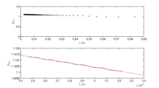
Figure 3: Domb-Sykes plot of Taylor series (A.1) using equation (4.14). The lower plot gives an amplified version of the large $m$ regime.

We now have good methods of estimating $r$ and $\theta$ for the singularity closest to the origin. However, the order of the singularity $\alpha$ does not appear in the approximation (4.10) and so we shall have to go back to either the exact expression (4.6) or the asymptotic result (4.9). Arguing from either of these results, keeping terms $O(1/m)$ but discarding terms $O(1/m^{2})$, we find that the approximation (4.11) is replaced by

$$B_{2m}=\frac{1}{r}\left(1-\frac{1+\alpha}{2m}\right).$$ (4.14)

In Figure 3 we plot $B_{2m}$ against $1/2m$ to obtain a standard Domb-Sykes [7] plot which, as predicted by (4.14), is approximately a straight line for large values of $m$. The best straight line fit to the data has intercept 1.1053876 and slope $-1.654448$ giving the estimates

$$r_{1}\approx 0.9047,\quad\alpha\approx 0.4967,$$ (4.15)

the first agreeing quite well with both the value $r_{1}\approx 0.905$ predicted by Table 1 and the value $r_{1}\approx 0.904$ of Itskov et al. [11]. We shall see that (4.15)₂ gives $\alpha$ correct to 2 dp.

The four singularities (4.2) may thus be approximated by

$$z\approx\pm 0.889\pm 0.166i.$$ (4.16)

4.2 Continued fraction representations and Padé approximants

A continued fraction representation can be calculated for any Taylor series and we are able to calculate the poles and zeros of this continued fraction. These poles and zeros are approximately equal to the poles and zeros calculated using the Padé approximant to the same Taylor series, see Hinch [9, pp 151–154] for a discussion of Padé approximants and continued fraction representations. Using Maple the continued fraction representation method takes less computational time than the Padé approximant method and so can be used to calculate a Taylor series expansion of a higher order. The largest Taylor series that we were able to work with was one of 150 terms.

Performing increasing truncations of $5,10,15\ldots 150$ terms of the continued fraction representation of the Taylor series (3.3) we obtain Figure 4 in which the black circle (which appears as an ellipse because of different axis scalings) has a radius of convergence of $0.905$. We have removed all the spurious pole-zero pairs (Froissart doublets) using the fitting criterion of Gonnet et al. [8]. From Figure 4 it can be seen that the sequence of poles tend to the circle of convergence of radius $0.905$. The singularity at $z_{1}$ in the first quadrant is identified in the subplot in Figure 4 by the red square. The line of poles radiating out along the real axis at $y=0$ demonstrates the existence of a branch cut at $x\approx 1$, see Hinch [9, p. 152].

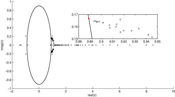
Figure 4: Plot of the singularities found using the continued fraction method, the black circle (which appears as an ellipse because of different axis scalings) has a radius convergence of $0.905$. The subplot identifies the location of the singularity at $z_{1}$ in the first quadrant.

5 Graphical representation of the inverse Langevin function

Before continuing with our discussion of the inverse Langevin function we exhibit Figure 5 which depicts the Langevin function itself in the complex plane showing the simple poles at $z=\pm in\pi$, $n=1,2,3,\dots$. The removable singularity at the origin is represented by the white square.

Figure 5: Plot of the simple poles of the Langevin function in the complex plane. The removable singularity at the origin shows as a white square.

5.1 At the initial radius of convergence $r_{1}$

Returning to the inverse Langevin function, Figure 6 is a three dimensional plot of this function in the complex plane specifically focusing on the singularity in the first quadrant as identified using the methods of subsection 4.1. The yellow and green surface is the inverse Langevin function and the wall of grey is part of a cylinder of radius $r_{1}=0.905$. Figure 6 clearly identifies a branch cut at $z_{1}\approx 0.889+0.166i$.

Performing an extensive numerical search of the surface plotted in Figure 6 at the radius of convergence $r_{1}=0.9046$ we identify a branch cut singularity at

$$z_{1}=0.88924042727+0.16622770313i$$ (5.1)

giving a more accurate estimate of the radius of convergence of $r_{1}=0.90464367946$. The further branch cuts at $-z_{1}$ and $\pm\bar{z}_{1}$ were also found by this method. These are more accurate values of the positions of the singularities given in equation (4.16). These accurate values were found using MATLAB’s built-in data cursor mode which allows data points to be read directly from a plot by displaying the position of the point selected.

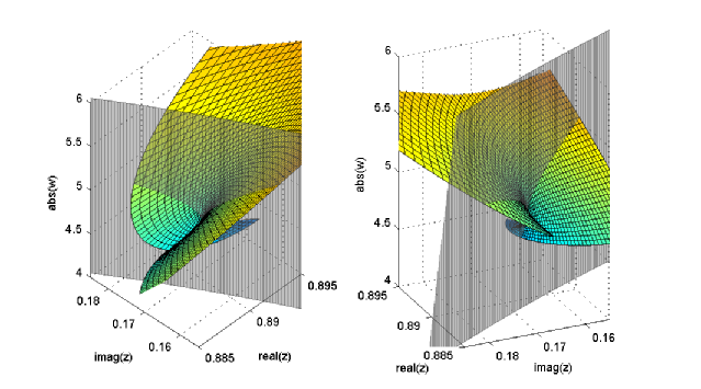
Figure 6: Plot of the inverse Langevin function $\mathscr{L}^{-1}(z)$ at the point $z=z_{1}=0.889+0.166i$ in the complex plane.

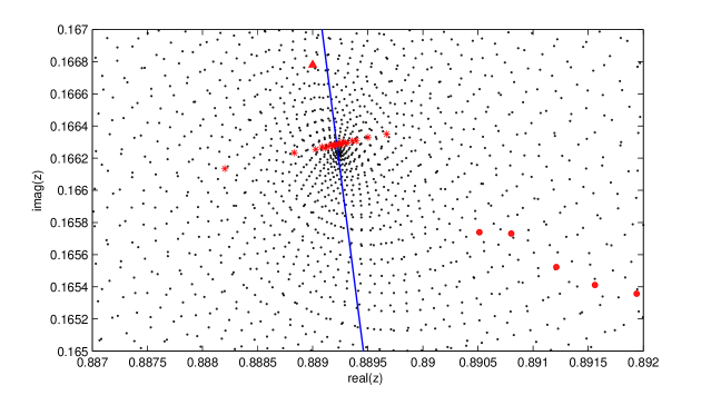
Figure 7: Singularity in the complex plane at $z=z_{1}$

Figure 7 represents a two dimensional plot of the complex plane close to the point $z=z_{1}$ with $z_{1}$ given by (5.1). The dense area of black dots represents the branch cut singularity. The blue curve is part of a circle at the the radius of convergence $r_{1}=0.9046436795$ which passes through the singularity at $z=z_{1}$. The red triangle marks the point $z_{1}=0.889+0.166i$ which is the approximate value of the singularity $z_{1}$ found using the Domb-Sykes method. The large red dots are the poles found using the continued fraction method and the red stars are the first 17 poles presented in Table 1. Recall that the largest continued fraction we could calculate was for the Taylor series (3.3) expanded to 150 terms.

Figure 8 represents three dimensional plots of the four singularities nearest to the origin. They were obtained using the same extensive numerical search methods that were used for Figure 6. They illustrate the nature of these singularities very clearly. They are typical square root singularities.

Figure 8: Plot of the four complex conjugate branch cut singularities of $\mathscr{L}^{-1}(z)$ closest to the origin

5.2 At the second radius of convergence $r_{2}$

Following the upper branch of the poles found using the continued fraction of the Taylor series (3.3) as shown in the subplot of Figure 4, we identify a new branch cut at radius of convergence $r_{2}=0.9573$. A graphical representation of this branch cut is shown in Figure 9.

Figure 9: Plot of the inverse Langevin function $\mathscr{L}^{-1}(z)$ at the point $z=z_{2}=0.951+0.112i$ in the complex plane.

Using MATLAB’s built-in data cursor mode as before on the surface plotted in Figure 9 at $r_{2}=0.9573$ we identify a branch cut singularity at

$$z_{2}=0.95070539169+0.11225248497i,\\$$ (5.2)

giving a radius of convergence of $r_{2}=0.95730943909$ and further branch cuts at $-z_{2}$ and $\pm\bar{z}_{2}$.

5.3 Removal to infinity of the nearest complex singularities by Euler’s method

Each of the four singularities $z=\pm r_{1}{\rm e}^{\pm i\theta_{1}}$ given at (4.2) is a zero of the quartic expression

$$z^{4}-4z^{2}r_{1}^{2}\cos 2\theta_{1}+r_{1}^{4}$$ (5.3)

and so the Euler transformation

$$\hat{z}=\frac{z}{\left(z^{4}-4z^{2}r_{1}^{2}\cos 2\theta_{1}+r_{1}^{4}\right)^{1/4}}$$ (5.4)

removes each of these singularities to infinity. This is an extension of the method of Van Dyke [25, p. 294] for removing a pair of complex conjugate singularities. We do not pursue this method here.

6 Exact analysis of the complex singularities of the inverse Langevin function.

We extend the definition (1.2) of the inverse Langevin function to the complex plane by

$$z=\mathscr{L}(w)=\coth w-1/w\quad\mbox{so that}\quad w=\mathscr{L}^{-1}(z),$$ (6.1)

where $w=u+iv$ and $z=x+iy$ with $u,v,x,y$ real.

6.1 Identifying the complex singularities of $\mathscr{L}^{-1}$

Singularities occur when $dw/dz=0$ or $\infty$. We find that

$$\frac{dz}{dw}=\frac{1}{w^{2}}-\frac{1}{\sinh^{2}w}$$ (6.2)

so that

$$\frac{dz}{dw}=0\implies\sinh w=\pm w.$$ (6.3)

Since $w=0$ is a removable singularity of the righthand side of (6.2), the relevant root of (6.3) closest to the origin in the first quadrant is

$$w_{1}=u_{1}+iv_{1}=2.250728612+4.212392230i,$$ (6.4)

which satisfies $\sinh w_{1}=-w_{1}$ correct to 9 dp and gives rise to the branch point of $\mathscr{L}^{-1}$ at

$$z_{1}=x_{1}+iy_{1}=\mathscr{L}(w_{1})=0.889240427+0.166227703i.$$ (6.5)

Then the radius of convergence $r_{1}$ of the Taylor series (3.2) of $\mathscr{L}^{-1}(z)$ is $r_{1}=|z_{1}|=0.904643679$ correct to 9 dp. Previous estimates of $r_{1}$ agree quite well with this value: $r_{1}\approx 0.904$ of [11], $r_{1}\approx 0.905$ predicted by Table 1, $r_{1}\approx 0.905$ from the method of Padé approximants, and $r_{1}\approx 0.9047$ estimated at (4.15) by the Domb-Sykes method.

Each $w_{n}$ satisfies the equation

$$\sinh w_{n}-(-1)^{n}w_{n}=0.$$ (6.6)

The same equation is satisfied by $-w_{n}$ and by $\pm\overline{w}_{n}$, with overbar denoting complex conjugate. This means that every root $w_{n}$ of $dz/dw=0$ in the first quadrant generates another root in each of the other three quadrants. The first 100 roots $w_{n}$ of equation (6.6) in the first quadrant and the corresponding branch points $z_{n}$ have been calculated to 15 significant figures and are exhibited in Tables 3 and 4. From these tables we can read off the values $r_{1}=0.904643679457684$ and $r_{2}=0.957309439091278$ for the radius of convergence $r_{1}$ of the Taylor series (3.2) and the distance from the origin $r_{2}$ of the singularities next-nearest the origin.

From (6.2) and the definition (6.1) we find that

$$\frac{dz}{dw}=1-\frac{2z}{w}-z^{2}.$$ (6.7)

At the $n^{\rm th}$ branch cut we have $w=w_{n}$, $z=z_{n}$ and ${dz}/{dw}|_{w_{n}}=0$ so that (6.7) reduces to

$$w_{n}=\frac{2z_{n}}{1-z_{n}^{2}}\quad\mbox{for}\quad n=1,2,\dots,$$ (6.8)

which can be verified to hold to a high degree of accuracy for the $w_{n}$, $z_{n}$ given in Tables 3 and 4.

n	$w_{n}=u_{n}+iv_{n}$	$z_{n}=x_{n}+iy_{n}$	$|z_{n}|$
1	2.25072861160186 $+$ 4.21239223049066$\hskip 1.42262pti$	0.889240427271280 $+$ 0.1662277031337704$\hskip 1.42262pti$	0.904643679457684
3	3.10314874582525 $+$ 10.7125373972793$\hskip 1.42262pti$	0.971651895822876 $+$ 0.0839661146033054$\hskip 1.42262pti$	0.975273148947393
5	3.55108734702208 $+$ 17.0733648531518$\hskip 1.42262pti$	0.986814304663841 $+$ 0.0554855076774800$\hskip 1.42262pti$	0.988372962727839
7	3.85880899310557 $+$ 23.3983552256513$\hskip 1.42262pti$	0.992296030564516 $+$ 0.0413207082174984$\hskip 1.42262pti$	0.993155986339352
9	4.09370492476533 $+$ 29.7081198252760$\hskip 1.42262pti$	0.994912673628922 $+$ 0.0328831365761801$\hskip 1.42262pti$	0.995455940169397
11	4.28378158777502 $+$ 36.0098660163716$\hskip 1.42262pti$	0.996372859485583 $+$ 0.0272934220634301$\hskip 1.42262pti$	0.996746610732843
13	4.44344583032427 $+$ 42.3068267176394$\hskip 1.42262pti$	0.997274223001842 $+$ 0.0233215298311909$\hskip 1.42262pti$	0.997546875899872
15	4.58110457345344 $+$ 48.6006841240946$\hskip 1.42262pti$	0.997871456587447 $+$ 0.0203554217132478$\hskip 1.42262pti$	0.998079048505216
17	4.70209646036170 $+$ 54.8924057880692$\hskip 1.42262pti$	0.998288513448522 $+$ 0.0180567357011610$\hskip 1.42262pti$	0.998451802435872
19	4.81002513746347 $+$ 61.1825901968339$\hskip 1.42262pti$	0.998591798634621 $+$ 0.0162233709022679$\hskip 1.42262pti$	0.998723574400725
21	4.90743841652255 $+$ 67.4716286349754$\hskip 1.42262pti$	0.998819578715363 $+$ 0.0147272406524697$\hskip 1.42262pti$	0.998928146786529
23	4.99620440987113 $+$ 73.7597883468280$\hskip 1.42262pti$	0.998995207952555 $+$ 0.0134832643013575$\hskip 1.42262pti$	0.999086194443897
25	5.07773373223829 $+$ 80.0472584358892$\hskip 1.42262pti$	0.999133616637730 $+$ 0.0124327312137003$\hskip 1.42262pti$	0.999210967064024
27	5.15311770138603 $+$ 86.3341766904029$\hskip 1.42262pti$	0.999244722640744 $+$ 0.0115338272465116$\hskip 1.42262pti$	0.999311285284185
29	5.22321798924776 $+$ 92.6206460143294$\hskip 1.42262pti$	0.999335329886089 $+$ 0.0107559689029146$\hskip 1.42262pti$	0.999393212117022
31	5.28872685705572 $+$ 98.9067448937676$\hskip 1.42262pti$	0.999410236024302 $+$ 0.0100762727169390$\hskip 1.42262pti$	0.999461030326854
33	5.35020884862568 $+$ 105.192534289525$\hskip 1.42262pti$	0.999472905159809 $+$ 0.0094772770169737$\hskip 1.42262pti$	0.999517837223650
35	5.40813039638030 $+$ 111.478062307910$\hskip 1.42262pti$	0.999525890748739 $+$ 0.0089454269554641$\hskip 1.42262pti$	0.999565919257192
37	5.46288131610703 $+$ 117.763367445661$\hskip 1.42262pti$	0.999571109526232 $+$ 0.0084700403806674$\hskip 1.42262pti$	0.999606995065338
39	5.51479071941834 $+$ 124.048480894101$\hskip 1.42262pti$	0.999610023661935 $+$ 0.0080425855175257$\hskip 1.42262pti$	0.999642377346630
41	5.56413899815659 $+$ 130.333428207196$\hskip 1.42262pti$	0.999643764736604 $+$ 0.0076561660632983$\hskip 1.42262pti$	0.999673083190480
43	5.61116698984546 $+$ 136.618230530152$\hskip 1.42262pti$	0.999673219886808 $+$ 0.0073051474114691$\hskip 1.42262pti$	0.999699910842030
45	5.65608308427746 $+$ 142.902905518431$\hskip 1.42262pti$	0.999699092784112 $+$ 0.0069848808630987$\hskip 1.42262pti$	0.999723494109270
47	5.69906880245861 $+$ 149.187468034869$\hskip 1.42262pti$	0.999721947529467 $+$ 0.0066914971210470$\hskip 1.42262pti$	0.999744341572300
49	5.74028322578860 $+$ 155.471930685222$\hskip 1.42262pti$	0.999742240733079 $+$ 0.0064217495837072$\hskip 1.42262pti$	0.999762865270417
51	5.77986654860470 $+$ 161.756304234369$\hskip 1.42262pti$	0.999760345286377 $+$ 0.0061728939730420$\hskip 1.42262pti$	0.999779401981825
53	5.81794295439426 $+$ 168.040597933200$\hskip 1.42262pti$	0.999776568202020 $+$ 0.0059425948368215$\hskip 1.42262pti$	0.999794229208793
55	5.85462296453648 $+$ 174.324819777869$\hskip 1.42262pti$	0.999791164158752 $+$ 0.0057288521782264$\hskip 1.42262pti$	0.999807577325354
57	5.89000537155756 $+$ 180.608976717251$\hskip 1.42262pti$	0.999804345895960 $+$ 0.0055299433342712$\hskip 1.42262pti$	0.999819638907802
59	5.92417884209128 $+$ 186.893074820336$\hskip 1.42262pti$	0.999816292270085 $+$ 0.0053443765303652$\hskip 1.42262pti$	0.999830575972350
61	5.95722325502924 $+$ 193.177119412340$\hskip 1.42262pti$	0.999827154556475 $+$ 0.0051708534637630$\hskip 1.42262pti$	0.999840525640985
63	5.98921082568168 $+$ 199.461115186172$\hskip 1.42262pti$	0.999837061421065 $+$ 0.0050082389329232$\hskip 1.42262pti$	0.999849604614774
65	6.02020705574268 $+$ 205.745066294327$\hskip 1.42262pti$	0.999846122874077 $+$ 0.0048555360122809$\hskip 1.42262pti$	0.999857912733750
67	6.05027154047907 $+$ 212.028976425124$\hskip 1.42262pti$	0.999854433437650 $+$ 0.0047118656262774$\hskip 1.42262pti$	0.999865535830996
69	6.07945865814335 $+$ 218.312848866321$\hskip 1.42262pti$	0.999862074701456 $+$ 0.0045764496394105$\hskip 1.42262pti$	0.999872548036799
71	6.10781816164831 $+$ 224.596686558490$\hskip 1.42262pti$	0.999869117398106 $+$ 0.0044485967760410$\hskip 1.42262pti$	0.999879013651023
73	6.13539568867313 $+$ 230.880492140035$\hskip 1.42262pti$	0.999875623098991 $+$ 0.0043276908325902$\hskip 1.42262pti$	0.999884988673966
75	6.16223320333355 $+$ 237.164267985343$\hskip 1.42262pti$	0.999881645608026 $+$ 0.0042131807582873$\hskip 1.42262pti$	0.999890522065250
77	6.18836938014610 $+$ 243.448016237264$\hskip 1.42262pti$	0.999887232113431 $+$ 0.0041045722678650$\hskip 1.42262pti$	0.999895656784726
79	6.21383993910375 $+$ 249.731738834892$\hskip 1.42262pti$	0.999892424144466 $+$ 0.0040014207171476$\hskip 1.42262pti$	0.999900430657599
81	6.23867793914730 $+$ 256.015437537410$\hskip 1.42262pti$	0.999897258370095 $+$ 0.0039033250251526$\hskip 1.42262pti$	0.999904877096959
83	6.26291403608140 $+$ 262.299113944652$\hskip 1.42262pti$	0.999901767268770 $+$ 0.0038099224676771$\hskip 1.42262pti$	0.999909025710048
85	6.28657670998225 $+$ 268.582769514888$\hskip 1.42262pti$	0.999905979692632 $+$ 0.0037208842000094$\hskip 1.42262pti$	0.999912902809196
87	6.30969246632743 $+$ 274.866405580268$\hskip 1.42262pti$	0.999909921344788 $+$ 0.0036359113923740$\hskip 1.42262pti$	0.999916531844230
89	6.33228601440944 $+$ 281.150023360279$\hskip 1.42262pti$	0.999913615184637 $+$ 0.0035547318824756$\hskip 1.42262pti$	0.999919933769883
91	6.35438042604379 $+$ 287.433623973499$\hskip 1.42262pti$	0.999917081773447 $+$ 0.0034770972661930$\hskip 1.42262pti$	0.999923127359161
93	6.37599727712690 $+$ 293.717208447911$\hskip 1.42262pti$	0.999920339570038 $+$ 0.0034027803609515$\hskip 1.42262pti$	0.999926129471595
95	6.39715677422076 $+$ 300.000777729961$\hskip 1.42262pti$	0.999923405184657 $+$ 0.0033315729872513$\hskip 1.42262pti$	0.999928955283640
97	6.41787786802549 $+$ 306.284332692552$\hskip 1.42262pti$	0.999926293597703 $+$ 0.0032632840227542$\hskip 1.42262pti$	0.999931618487311
99	6.43817835533659 $+$ 312.567874142105$\hskip 1.42262pti$	0.999929018348732 $+$ 0.0031977376906519$\hskip 1.42262pti$	0.999934131461767

Table 3: Solutions $w_{n}$ of $\sinh w=-w$ in the first quadrant and the corresponding branch points $z_{n}=\mathscr{L}(w_{n})$.

n	$w_{n}=u_{n}+iv_{n}$	$z_{n}=x_{n}+iy_{n}$	$|z_{n}|$
2	2.76867828298732 $+$ 7.49767627777639$\hskip 1.42262pti$	0.9507053916921612 $+$ 0.1122524849645265$\hskip 1.42262pti$	0.957309439091278
4	3.35220988485350 $+$ 13.8999597139765$\hskip 1.42262pti$	0.9814249275768375 $+$ 0.0668711449824057$\hskip 1.42262pti$	0.983700482108482
6	3.71676767975250 $+$ 20.2385177078300$\hskip 1.42262pti$	0.9901175152938447 $+$ 0.0473785974133679$\hskip 1.42262pti$	0.991250435351488
8	3.98314164033996 $+$ 26.5545472654916$\hskip 1.42262pti$	0.9938124512702532 $+$ 0.0366260858125753$\hskip 1.42262pti$	0.994487133381694
10	4.19325147043121 $+$ 32.8597410050699$\hskip 1.42262pti$	0.9957375998196626 $+$ 0.0298302646937089$\hskip 1.42262pti$	0.996184326511073
12	4.36679511767062 $+$ 39.1588165200650$\hskip 1.42262pti$	0.9968730165101870 $+$ 0.0251523955760530$\hskip 1.42262pti$	0.997190279760755
14	4.51464044948130 $+$ 45.4540714643551$\hskip 1.42262pti$	0.9976012288775898 $+$ 0.0217381656303724$\hskip 1.42262pti$	0.997838042822106
16	4.64342795705190 $+$ 51.7467683028218$\hskip 1.42262pti$	0.9980974683847858 $+$ 0.0191375308460208$\hskip 1.42262pti$	0.998280923128856
18	4.75751511808162 $+$ 58.0376620590943$\hskip 1.42262pti$	0.9984515279054803 $+$ 0.0170911687514174$\hskip 1.42262pti$	0.998597797727432
20	4.85991664789710 $+$ 64.3272337132856$\hskip 1.42262pti$	0.9987134143666453 $+$ 0.0154392353115651$\hskip 1.42262pti$	0.998832745770225
22	4.95280535741894 $+$ 70.6158050613296$\hskip 1.42262pti$	0.9989128315092538 $+$ 0.0140778854034248$\hskip 1.42262pti$	0.999012027861160
24	5.03779919329181 $+$ 76.9036000092884$\hskip 1.42262pti$	0.9990683548450882 $+$ 0.0129367469874774$\hskip 1.42262pti$	0.999152109078237
26	5.11613546596693 $+$ 83.1907794378375$\hskip 1.42262pti$	0.9991920999701078 $+$ 0.0119664511932357$\hskip 1.42262pti$	0.999263753268793
28	5.18878162856979 $+$ 89.4774620851630$\hskip 1.42262pti$	0.9992922511676224 $+$ 0.0111313467283301$\hskip 1.42262pti$	0.999354246563069
30	5.25650846760145 $+$ 95.7637376020254$\hskip 1.42262pti$	0.9993745037000536 $+$ 0.0104050483334986$\hskip 1.42262pti$	0.999428668628508
32	5.31994004501781 $+$ 102.049675012746$\hskip 1.42262pti$	0.9994429230481451 $+$ 0.0097676120844439$\hskip 1.42262pti$	0.999490651620540
34	5.37958872776665 $+$ 108.335328370326$\hskip 1.42262pti$	0.9995004761610887 $+$ 0.0092036840636058$\hskip 1.42262pti$	0.999542850330383
36	5.43588034897744 $+$ 114.620740638271$\hskip 1.42262pti$	0.9995493706262943 $+$ 0.0087012525134125$\hskip 1.42262pti$	0.999587242873138
38	5.48917265997610 $+$ 120.905946417967$\hskip 1.42262pti$	0.9995912773595068 $+$ 0.0082507858904696$\hskip 1.42262pti$	0.999625328431118
40	5.53976911179991 $+$ 127.190973904692$\hskip 1.42262pti$	0.9996274804707284 $+$ 0.0078446244699579$\hskip 1.42262pti$	0.999658260529732
42	5.58792931680847 $+$ 133.475846316267$\hskip 1.42262pti$	0.9996589803554569 $+$ 0.0074765425850377$\hskip 1.42262pti$	0.999686938843525
44	5.63387710617850 $+$ 139.760582953693$\hskip 1.42262pti$	0.9996865660131676 $+$ 0.0071414281811005$\hskip 1.42262pti$	0.999712073681050
46	5.67780681724206 $+$ 146.045200000247$\hskip 1.42262pti$	0.9997108666807187 $+$ 0.0068350445868388$\hskip 1.42262pti$	0.999734232080716
48	5.71988825776711 $+$ 152.329711131562$\hskip 1.42262pti$	0.9997323892895176 $+$ 0.0065538509093109$\hskip 1.42262pti$	0.999753871288464
50	5.76027066783195 $+$ 158.614127987106$\hskip 1.42262pti$	0.9997515460351737 $+$ 0.0062948648906245$\hskip 1.42262pti$	0.999771363424514
52	5.79908591278778 $+$ 164.898460538558$\hskip 1.42262pti$	0.9997686749398286 $+$ 0.0060555569619736$\hskip 1.42262pti$	0.999787013898991
54	5.83645107971304 $+$ 171.182717380588$\hskip 1.42262pti$	0.9997840553752877 $+$ 0.0058337675202634$\hskip 1.42262pti$	0.999801075327556
56	5.87247060628390 $+$ 177.466905962516$\hskip 1.42262pti$	0.9997979199133771 $+$ 0.0056276416996543$\hskip 1.42262pti$	0.999813758164097
58	5.90723803960322 $+$ 183.751032774485$\hskip 1.42262pti$	0.9998104634661614 $+$ 0.0054355774695200$\hskip 1.42262pti$	0.999825238908704
60	5.94083749958616 $+$ 190.035103498259$\hskip 1.42262pti$	0.9998218504033833 $+$ 0.0052561839878047$\hskip 1.42262pti$	0.999835666504330
62	5.97334490452427 $+$ 196.319123130293$\hskip 1.42262pti$	0.9998322201440941 $+$ 0.0050882479216131$\hskip 1.42262pti$	0.999845167366018
64	6.00482900375061 $+$ 202.603096082861$\hskip 1.42262pti$	0.9998416915859598 $+$ 0.0049307060121844$\hskip 1.42262pti$	0.999853849367623
66	6.03535225272971 $+$ 208.887026267693$\hskip 1.42262pti$	0.9998503666409769 $+$ 0.0047826225743309$\hskip 1.42262pti$	0.999861805026467
68	6.06497155857294 $+$ 215.170917165564$\hskip 1.42262pti$	0.9998583330782893 $+$ 0.0046431709252659$\hskip 1.42262pti$	0.999869114065604
70	6.09373891834152 $+$ 221.454771884529$\hskip 1.42262pti$	0.9998656668253923 $+$ 0.0045116179650518$\hskip 1.42262pti$	0.999875845489253
72	6.12170196812237 $+$ 227.738593208909$\hskip 1.42262pti$	0.9998724338427762 $+$ 0.0043873113019690$\hskip 1.42262pti$	0.999882059274561
74	6.14890445743776 $+$ 234.022383640710$\hskip 1.42262pti$	0.9998786916602354 $+$ 0.0042696684459880$\hskip 1.42262pti$	0.999887807758862
76	6.17538666085092 $+$ 240.306145434805$\hskip 1.42262pti$	0.9998844906430244 $+$ 0.0041581676929462$\hskip 1.42262pti$	0.999893136783638
78	6.20118573648736 $+$ 246.589880628955$\hskip 1.42262pti$	0.9998898750409366 $+$ 0.0040523403987275$\hskip 1.42262pti$	0.999898086642878
80	6.22633603948128 $+$ 252.873591069537$\hskip 1.42262pti$	0.9998948838619153 $+$ 0.0039517644023399$\hskip 1.42262pti$	0.999902692873224
82	6.25086939698059 $+$ 259.157278433673$\hskip 1.42262pti$	0.9998995516030284 $+$ 0.0038560584034185$\hskip 1.42262pti$	0.999906986915457
84	6.27481535023279 $+$ 265.440944248347$\hskip 1.42262pti$	0.9999039088648717 $+$ 0.0037648771364091$\hskip 1.42262pti$	0.999910996670755
86	6.29820136836983 $+$ 271.724589906972$\hskip 1.42262pti$	0.9999079828702210 $+$ 0.0036779072127901$\hskip 1.42262pti$	0.999914746970491
88	6.32105303777144 $+$ 278.008216683796$\hskip 1.42262pti$	0.9999117979036525 $+$ 0.0035948635258953$\hskip 1.42262pti$	0.999918259974626
90	6.34339423028012 $+$ 284.291825746477$\hskip 1.42262pti$	0.9999153756856314 $+$ 0.0035154861314920$\hskip 1.42262pti$	0.999921555510870
92	6.36524725303997 $+$ 290.575418167091$\hskip 1.42262pti$	0.9999187356920239 $+$ 0.0034395375322614$\hskip 1.42262pti$	0.999924651364477
94	6.38663298231693 $+$ 296.858994931788$\hskip 1.42262pti$	0.9999218954279676 $+$ 0.0033668003064646$\hskip 1.42262pti$	0.999927563526761
96	6.40757098331232 $+$ 303.142556949306$\hskip 1.42262pti$	0.9999248706634182 $+$ 0.0032970750309580$\hskip 1.42262pti$	0.999930306408908
98	6.42807961769295 $+$ 309.426105058477$\hskip 1.42262pti$	0.9999276756363949 $+$ 0.0032301784568029$\hskip 1.42262pti$	0.999932893026560
100	6.44817614031860 $+$ 315.709640034877$\hskip 1.42262pti$	0.9999303232289011 $+$ 0.0031659419023442$\hskip 1.42262pti$	0.999935335159621

Table 4: Solutions $w_{n}$ of $\sinh w=w$ in the first quadrant and the corresponding branch points $z_{n}=\mathscr{L}(w_{n})$.

6.2 Power series for $w$ close to the first singularity $z=z_{1}$

We expand $z=\mathscr{L}(w)$ as a power series about the point $w_{1}$ which is possible since $\mathscr{L}$ is analytic everywhere in the complex plane except at its poles $w=\pm n\pi i,\;n=1,2,\ldots$.

$$z=\mathscr{L}(w_{1}+(w-w_{1}))=\mathscr{L}(w_{1})+(w-w_{1})\frac{d\mathscr{L}}{dw}\Big{|}_{w=w_{1}}+\frac{1}{2}(w-w_{1})^{2}\frac{d^{2}\mathscr{L}}{dw^{2}}\Big{|}_{w=w_{1}}+\cdots$$ (6.9)

At $w=w_{1}$, we have $z=z_{1}$, ${d\mathscr{L}}/{dw}=0$ and, by differentiating (6.7), ${d^{2}\mathscr{L}}/{dw^{2}}=2{z_{1}}/{w_{1}^{2}}$, so the series (6.9) becomes

$$z-z_{1}=\frac{z_{1}}{w_{1}^{2}}(w-w_{1})^{2}+O\left((w-w_{1})^{3}\right).$$ (6.10)

Taking $w-w_{1}$ small in (6.10) we see that $z-z_{1}$ and $(w-w_{1})^{2}$ must balance. Therefore the series for $w$ must take the form

$$w-w_{1}=\frac{w_{1}}{\sqrt{z}_{1}}(z-z_{1})^{1/2}+\cdots$$ (6.11)

and continues as a power series in $(z-z_{1})^{1/2}$. The appearance of the exponent $1/2$ in (6.11) perhaps explains the exponent $\alpha\approx 1/2$ in the Domb-Sykes plots, see (4.15), and the typical square root nature of the plots in Figure 8.

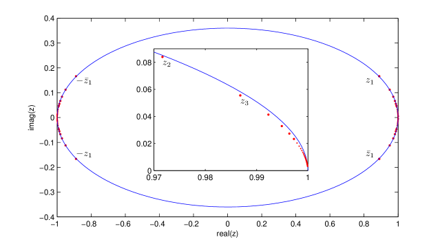
Figure 10: The branch cut singularities lie approximately on the ellipse $x^{2}+y^{2}/(0.36)^{2}=1$. The inset shows the accumulation point of singularities at $z=1$.

On writing $w_{n}=u_{n}+iv_{n}$ we observe the following approximations from Tables 3 and 4

$$v_{n}\approx(n+\tfrac{1}{2})\pi\quad\mbox{and}\quad u_{n}\approx\sinh^{-1}v_{n}.$$ (6.12)

We further observe empirically that the branch cuts at $z_{n}=x_{n}+iy_{n}$ given in Tables 3 and 4 lie approximately on the ellipse

$$x^{2}+y^{2}/(0.36)^{2}=1.$$ (6.13)

This is illustrated in Figure 10.

7 Conclusions

The inverse Langevin function has been used extensively in the modern literature, spanning nearly 80 years, to model the limited-stretch elasticity of rubber and rubber-like materials beginning with the original single chain model of Kuhn & Grün [17]. We give a Taylor series for the inverse Langevin function and note that its only real singularities are two simple poles at $x=\pm 1$, each with residue $-1$. We have seen that the effects of these poles may be removed either multiplicatively or additively but it is evident there remain complex singularities.

In Section 4 we extended the methods of Hunter & Guerrieri [10] and Mercer & Roberts [19] in the two-singularity case to the present situation of four complex singularities equidistant from the origin and of equal strength and then developed an algorithm for estimating the four complex singularities with the smallest radius of convergence. Using these algorithms and excluding the two outliers from the sequence $2m=264..280$ presented in Table 1, we find that the average values of $r=0.9047$ and $\cos 2\theta=0.9324$ obtained from eq.(4.1) are correct to 0.01%, demonstrating excellent agreement between the new algorithm and the exact values found in Section 6. From the Domb-Sykes [7] plot the radius of convergence is estimated to be $r=0.9047$ and the order of the singularity is estimated to be $\alpha=0.50$, correct to 2 dp. Also in Section 4 we used the method of Padé approximants to show that the positions of the poles tend to imply a radius of convergence of $r_{1}\approx 0.905$, see Figure 4. Itskov et al. [11] had earlier used the Taylor series (3.2) to estimate its radius of convergence to be $r_{1}\approx 0.904$. These estimates of the radius of convergence compare well with the exact value $r_{1}\approx 0.9046$, correct to 4dp, found in Section 6.

As an illustrative example of the complex singularities, in Section 5 we presented a graphical representation of the four singularities nearest the origin which points to these complex singularities being of a square root nature, see Figure 8. These methods were then used to discuss and illustrate the branch cut singularities which are the next-nearest to the origin.

An exact analysis of the complex singularities of the inverse Langevin function was given in Section 6. We found that $\mathscr{L}^{-1}(x)$ has an infinity of complex singularities. The complex singularities have been identified as square root branch points and the first 100 are given in Tables 3 and 4 correct to 15 significant figures. From these tables we can read off the values $r_{1}=0.904643679457684$ and $r_{2}=0.957309439091278$ for the radius of convergence $r_{1}$ of the Taylor series (3.2) and the distance from the origin $r_{2}$ of the singularities next-nearest the origin.

Appendix A Power series expansion for h(x) defined by (3.7)

$$h(x)= \,1.000000000-0.200000000x^{2}-0.302857143x^{4}-0.241142857x^{6}$$ (A.1)

$$-0.128133581x^{8}-0.002754320x^{10}+0.112823652x^{12}+0.202302872x^{14}$$

$$+0.252957871x^{16}+0.255767493x^{18}+0.206400668x^{20}+0.106427839x^{22}$$

$$-0.035638662x^{24}-0.203814671x^{26}-0.374937806x^{28}-0.520051694x^{30}$$

$$-0.607058580x^{32}-0.604674268x^{34}-0.487519715x^{36}-0.241938122x^{38}$$

$$+0.128142774x^{40}+0.596240341x^{42}+1.11037244x^{44}+1.59335189x^{46}$$

$$+1.94743654x^{48}+2.06412582x^{50}+1.83930767x^{52}+1.19311006x^{54}$$

$$+0.092746229x^{56}-1.42453659x^{58}-3.23242249x^{60}-5.10527925x^{62}$$

$$-6.72188993x^{64}-7.68786819x^{66}-7.57992954x^{68}-6.01247167x^{70}$$

$$-2.72302819x^{72}+2.33166258x^{74}+8.88247800x^{76}+16.2760008x^{78}$$

$$+23.4457067x^{80}+28.9488707x^{82}+31.0887121x^{84}+28.1332646x^{86}$$

$$+18.6289734x^{88}+1.78834329x^{90}-22.0915299x^{92}-51.2463614x^{94}$$

$$-82.1856215x^{96}-109.657418x^{98}-126.936675x^{100}-126.515484x^{102}$$

$$-101.230289x^{104}-45.7910264x^{106}+41.4148208x^{108}+156.476988x^{110}$$

$$+288.416518x^{112}+418.365849x^{114}+519.941655x^{116}+561.243625x^{118}$$

$$+508.779920x^{120}+333.372235x^{122}+17.7285206x^{124}-435.089332x^{126}$$

$$-993.583683x^{128}-1591.88222x^{130}-2128.03573x^{132}-2468.71682x^{134}$$

$$-2462.15815x^{136}-1960.33797x^{138}-850.028856x^{140}+909.598564x^{142}$$

$$+3247.43267x^{144}+5945.95697x^{146}+8620.94561x^{148}+10725.5600x^{150}$$

$$+11588.7216x^{152}+10495.1411x^{154}+6809.31069x^{156}+138.002694x^{158}$$

$$-9484.30277x^{160}-21414.1097x^{162}-34259.9150x^{164}-45832.1674x^{166}$$

$$-53231.6417x^{168}-53119.8507x^{170}-42197.9104x^{172}-17890.0779x^{174}$$

$$+20814.7257x^{176}+72462.7741x^{178}+132332.352x^{180}+191933.101x^{182}$$

$$+239044.368x^{184}+258526.027x^{186}+234083.723x^{188}+151058.955x^{190}$$

$$+138.520758x^{192}-218355.931x^{194}-490207.857x^{196}-783953.594x^{198}$$

$$-1049528.05x^{200}-1220084.59x^{202}-1218051.56x^{204}-966106.693x^{206}$$

$$-403058.159x^{208}+496382.913x^{210}+1700206.49x^{212}+3099711.64x^{214}$$

$$+4496983.88x^{216}+5604915.71x^{218}+6065463.63x^{220}+5490700.59x^{222}$$

$$+3528641.83x^{224}-48340.4005x^{226}-5240311.82x^{228}-11716162.1x^{230}$$

$$-18730611.2x^{232}-25088247.2x^{234}-29183447.1x^{236}-29142674.8x^{238}$$

$$-23086790.5x^{240}-9514471.49x^{242}+12216497.8x^{244}+41364045.0x^{246}$$

$$+75320486.9x^{248}+109294073.x^{250}+136293596.x^{252}+147558398.x^{254}$$

$$+133549963.x^{256}+85559226.7x^{258}-2117991.14x^{260}-129623899.x^{262}$$

$$-288950873.x^{264}-461841775.x^{266}-618836155.x^{268}-720187300.x^{270}$$

$$-719324164.x^{272}-569318735.x^{274}-232412338.x^{276}+307951890.x^{278}$$

$$+0.103391594e10x^{280}+0.188099576e10x^{282}+0.272985768e10x^{284}+0.340562715e10x^{286}$$

$$+0.368836021e10x^{288}+0.333768440e10x^{290}+0.213308037e10x^{292}-71274982.4x^{294}$$

$$-0.328169584e10x^{296}-0.729899021e10x^{298}-0.116643883e11x^{300}-0.156341281e11x^{302}$$

$$-0.182012750e11x^{304}-0.181822064e11x^{306}-0.143799103e11x^{308}-0.582598386e10x^{310}$$

$$+0.791220705e10x^{312}+0.263925558e11x^{314}+0.479829063e11x^{316}+0.696458232e11x^{318}$$

$$+0.869147211e11x^{320}+0.941554975e11x^{322}+0.851924977e11x^{324}+0.543388085e11x^{326}$$

$$-0.219436431e10x^{328}-0.846249706e11x^{330}-0.187888503e12x^{332}-0.300224905e12x^{334}$$

$$-0.402497064e12x^{336}-0.468724442e12x^{338}-0.468288971e12x^{340}-0.370136642e12x^{342}$$

$$-0.149034695e12x^{344}+0.206455043e12x^{346}+0.685141918e12x^{348}+0.124494613e13x^{350}$$

$$+0.180719994e13x^{352}+0.225589644e13x^{354}+0.244436067e13x^{356}+0.221143352e13x^{358}$$

$$+0.140825874e13x^{360}-0.649324487e11x^{362}-0.221501096e13x^{364}-0.491094324e13x^{366}$$

$$-0.784640464e13x^{368}-0.105213812e14x^{370}-0.122555119e14x^{372}-0.122453010e14x^{374}$$

$$-0.967388504e13x^{376}-0.387516784e13x^{378}+0.545634834e13x^{380}+0.180323131e14x^{382}$$

$$+0.327515035e14x^{384}+0.475474135e14x^{386}+0.593656087e14x^{388}+0.643366501e14x^{390}$$

$$+0.582005673e14x^{392}+0.370127270e14x^{394}-0.188373561e13x^{396}-0.586963931e14x^{398}$$

$$-0.129986377e15x^{400}-0.207668859e15x^{402}-0.278513129e15x^{404}-0.324482299e15x^{406}$$

$$-0.324237662e15x^{408}-0.256042771e15x^{410}-0.102120719e15x^{412}+0.145760298e15x^{414}$$

$$+0.480061030e15x^{416}+0.871604193e15x^{418}+0.126546279e16x^{420}+0.158029270e16x^{422}$$

$$+0.171287647e16x^{424}+0.154939007e16x^{426}+0.984213300e15x^{428}-0.540858239e14x^{430}$$

$$-0.157163820e16x^{432}-0.347711790e16x^{434}-0.555478063e16x^{436}-0.745079732e16x^{438}$$

$$-0.868203472e16x^{440}-0.867606804e16x^{442}-0.684883117e16x^{444}-0.272146238e16x^{446}$$

$$+0.392956599e16x^{448}$$

References

- [1] E. M. Arruda and M. C. Boyce. A three-dimensional constitutive model for the large stretch behavior of rubber elastic materials. J. Mech. Phys. Solids, 41:389–412, 1993. (doi:10.1016/0022-5096(93)90013-6).
- [2] M. F. Beatty. An average-stretch full-network model for rubber elasticity. J. Elasticity, 70:65–86, 2003. (doi:10.1023/B:ELAS.0000005553.38563.91).
- [3] M. F. Beatty. On constitutive models for limited elastic, molecular based materials. Math. Mech. Solids, 13:375–387, 2008. (doi:10.1177/1081286507076405).
- [4] A. Cohen. A Padé approximant to the inverse Langevin function. Rheol. Acta, 30:270–273, 1991. (doi:10.1007/BF00366640).
- [5] E. Darabi and M. Itskov. A simple and accurate approximation of the inverse langevin function. Rheol. Acta, 54:455–459, 2015. (doi: 10.1007/s00397-015-0851-1).
- [6] R. A. Dickie and T. L. Smith. Viscoelastic properties of a rubber vulcanizate under large deformations in equal biaxial tension, pure shear, and simple tension. Trans. Soc. Rheol., 15:91–110, 1971.
- [7] C. Domb and M. F. Sykes. On the susceptibility of a ferromagnetic above the curie point. Proc. R. Soc. Lond. A., 240:214–228, 1957. (doi:10.1098/rspa.1957.0078).
- [8] P. Gonnet, S. Güttel, and L. N. Trefethen. Robust Padé approximation via SVD. SIAM review, 55:101–117, 2013. (doi:10.1137/110853236).
- [9] H. J. Hinch. Perturbation Methods. Cambridge University Press, Cambridge, 1995.
- [10] C. Hunter and B. Guerrieri. Deducing the properties of singularities of functions from their Taylor series coefficients. SIAM J. Appl. Math., 39:248–263, 1980. (doi:10.1137/0139022).
- [11] M. Itskov, R. Dargazany, and K. Hörnes. Taylor expansion of the inverse function with application to the Langevin function. Math. Mech. Solids, 17:693–671, 2012. (doi:10.1177/1081286511429886).
- [12] M. Itskov, A. E. Ehret, and R. Dargazany. A full-network rubber elasticity model based on analytical integration. Math. Mech. Solids, 15:655–671, 2010. (doi:10.1177/1081286509106441).
- [13] H. M. James and E. Guth. Theory of the elastic properties of rubber. J. Chem. Phys., 11:455–481, 1943. (doi:10.1063/1.1723785).
- [14] R. Jedynak. Approximation of the inverse langevin function revisited. Rheol. Acta, 54:29–39, 2015. (doi: 10.1007/s00397-014-0802-2).
- [15] R. Jedynak. New facts concerning the approximation of the inverse langevin function. J. Non-Newton. Fluid Mech., 249:8–25, 2017. (doi: 10.1016/j.nnfm.2017.09.003).
- [16] M. Kröger. Simple, admissible, and accurate approximants of the inverse langevin and brillouin functions, relevant for strong polymer deformations and flows. J. Non-Newton. Fluid Mech., 223:77–87, 2015. (doi: 10.1016/j.nnfm.2015.05.007).
- [17] W. Kuhn and F. Grün. Beziehungen zwischen elastischen Konstanten und Dehnungsdoppelbrechung hochelastischer Stoffe. Kolloid-Z, 101:248–271, 1942. (doi:10.1007/BF01793684).
- [18] B. C. Marchi and E. M. Arruda. An error-minimizing approach to inverse langevin approximations. Rheol. Acta, 54:887–902, 2015. (doi: 10.1007/s00397-015-0880-9).
- [19] G. N. Mercer and A. J. Roberts. A centre manifold description of contaminant dispersion in channels with varying flow properties. SIAM J. Appl. Math., 50:1547–1565, 1990. (doi:10.1137/0150091).
- [20] A. N. Nguessong, T. Beda, and P. Peyrault. A new based error approach to approximate the inverse langevin function. Rheol. Acta, 53:585–591, 2014. (doi: 10.1007/s00397-014-0778-y).
- [21] M. A. Puso. Mechanistic constitutive models for rubber elasticity and viscoelasticity. Doctoral dissertation, University of California, Davis, page 124 pages, 1994.
- [22] S. R. Rickaby and N. H. Scott. Orthotropic cyclic stress-softening model for pure shear during repeated loading and unloading. IMA J. Appl. Math., 79:869–888, 2014. doi:10.1093/imamat/hxu021.
- [23] S. R. Rickaby and N. H. Scott. A comparison of limited-stretch models of rubber elasticity. Int. J. Non-Linear Mech., 68:71–86, 2015. (doi:10.1016/j.ijnonlinmec.2014.06.009).
- [24] L. R. G. Treloar. The Physics of Rubber Elasticity. Clarendon Press, Oxford, 1975.
- [25] M Van Dyke. Computer-extended series. Ann. Rev. Fluid Mech., 16:287–309, 1984. (doi:10.1146/annurev.fl.16.010184.001443).
- [26] M. C. Wang and E. Guth. Statistical Theory of Networks of Non-Gaussian Flexible Chains. J. Chem. Phys., 20:1144–1157, 1952. (doi:10.1063/1.1700682).
- [27] P. D. Wu and E. Van der Giessen. On improved network models for rubber elasticity and their application to orientation hardening in glassy polymers. J. Mech. Phys. Solids, 41:427–456, 1993. (doi:10.1016/0022-5096(93)90043-F).
- [28] A. E. Zúñiga and M. F. Beatty. Constitutive equations for amended non-Gaussian network models of rubber elasticity. Int. J. Engng. Sci., 40:2265–2294, 2002. (doi:10.1016/S0020-7225(02)00140-4).