A Numerical Method for Determining the Elements of Circumbinary Orbits and Its Application to Circumbinary Planets and the Satellites of Pluto-Charon

Abstract

Planets and satellites orbiting a binary system exist in the solar system and extrasolar planetary systems. Their orbits can be significantly different from Keplerian orbits, if they are close to the binary and the secondary-to-primary mass ratio is high. A proper description of a circumbinary orbit is in terms of the free eccentricity $e_{\rm free}$ at the epicyclic frequency $\kappa_{0}$, forced eccentricity $e_{\rm forced}$ at the mean motion $n_{0}$, and oscillations at higher frequencies forced by the non-axisymmetric components of the binary’s potential. We show that accurate numerical values for the amplitudes and frequencies of these terms can be extracted from numerical orbit integrations by applying fast Fourier transformation (FFT) to the cylindrical distance between the circumbinary object and the center of mass of the binary as a function of time. We apply this method to three Kepler circumbinary planets and the satellites of Pluto-Charon. For the satellite Styx of Pluto-Charon, the FFT results for $\kappa_{0}$ and $e_{\rm free}$ differ significantly from the first-order analytic value and the value reported by Showalter & Hamilton (2015), respectively. We show that the deviation in $\kappa_{0}$ is likely due to the effect of the 3:1 mean-motion resonance and discuss the implications of the lower value for $e_{\rm free}$.

1 INTRODUCTION

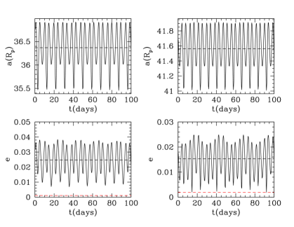
Figure 1: Evolution of the osculating semimajor axis $a_{\rm osc}$ in units of Pluto radius $R_{P}$ (upper panels) and eccentricity $e_{\rm osc}$ (lower panels) of the Pluto-Charon satellites Styx (left panels) and Nix (right panels). The black dashed lines indicate the mean values of $a_{\rm osc}$ and $e_{\rm osc}$, and the red dashed lines indicate the values of the free eccentricity $e_{\rm free}$.

Four small satellites – Styx, Nix, Kerberos and Hydra – are orbiting around Pluto-Charon, which is a binary system with Charon about $1/8$ of the mass of Pluto. Due to the non-spherical potential of the binary and the proximity of the satellites to the binary (with the orbital periods of the small satellites $\approx 3.16$–$5.98$ times that of Pluto-Charon), the orbits of the small satellites are significantly different from Keplerian orbits (Lee & Peale, 2006). To precisely describe a circumbinary orbit is not an easy task. Using the osculating Keplerian orbital elements may not be accurate enough, because they are calculated from the angular momentum and energy assuming a Keplerian orbit. Figure 1 shows the variations of the osculating semimajor axis $a_{\rm osc}$ and eccentricity $e_{\rm osc}$ for the two satellites closest to Pluto-Charon, Styx and Nix, using the best fit of Showalter & Hamilton (2015). We observe that both $a_{\rm osc}$ and $e_{\rm osc}$ have non-trivial variations on orbital timescales. The variation of $a_{\rm osc}$ is $\sim 4\%$ and $2\%$ for Styx and Nix, respectively. The percentage variation is calculated by $({\rm maximum}-{\rm minimum})/{\rm mean}\times 100\%$, and the mean value is indicated by the black dashed lines in the upper panels of Figure 1. For $e_{\rm osc}$, its lowest value can be more than 10 times smaller than the largest value within an orbital period. Also, the mean values of $e_{\rm osc}$, $\langle e_{\rm osc}\rangle$, and the free eccentricities $e_{\rm free}$ (which are indicated by the black and red dashed lines, respectively, in the lower panels of Figure 1) are significantly different from each other, where $e_{\rm free}$ is the appropriate generalization of eccentricity for circumbinary orbits (see below). The values of $e_{\rm free}$ shown in Figure 1 are those determined in Section 3.2 and listed in Table 2 below. Because of the variations in the osculating orbital elements and the significant difference between $\langle e_{\rm osc}\rangle$ and $e_{\rm free}$, the osculating elements do not provide clear information about the orbital evolution history of the system, and it is not suitable to use the instantaneous or mean value of the osculating elements to describe a circumbinary orbit. The orbital parameters reported by Brozović et al. (2015) and Showalter & Hamilton (2015) were obtained by an alternative method: fitting a precessing ellipse to the numerical integration of the best-fit orbit or the observational data, but it has not been demonstrated that the eccentricity obtained in this way should agree with $e_{\rm free}$.

Besides Pluto-Charon in the solar system, binary stars are frequently observed in the Milky Way. A number of exoplanets orbiting around binary stars have been discovered. Currently, there are about 20 of them, including Kepler-16 b, Kepler-34 b, and Kepler-35 b. Kepler-16 b was the first circumbinary exoplanet discovered by the Kepler spacecraft and it is a Saturn-mass planet orbiting around a binary with a total mass of $0.89M_{\odot}$, where $M_{\odot}$ is the solar mass (Doyle et al. 2011). This was quickly followed by the discovery of Kepler-34 b and Kepler-35 b (Welsh et al. 2012). Kepler-34 b is $0.22M_{\rm J}$ and orbits a pair of stars with masses similar to the Sun, while Kepler-35 b is about half the mass of Kepler-34 b ($0.13M_{\rm J}$) and orbits a binary with masses $0.89M_{\odot}$ and $0.81M_{\odot}$. One of the more recent discovery is Kepler-1647 b, which is the largest circumbinary Kepler planet known and has the longest period for any confirmed transiting circumbinary exoplanets (Kostov et al. 2016). A major difference between Pluto-Charon and the binary stars with circumbinary planets is that the orbit of the present-day Pluto-Charon is circular, while the orbits of the binary stars are eccentric.

Since circumbinary orbits can be significantly non-Keplerian, an analytic theory has to be developed to describe them. Lee & Peale (2006) showed that the motion of a test particle orbiting around a circular binary can be represented by the superposition of the circular motion of the guiding center, the epicyclic motion, the forced oscillations due to the non-axisymmetric components of the binary’s potential, and the vertical motion. This theory is first order in terms of deviations from the uniform circular motion of the guiding center. Leung & Lee (2013) extended this theory to describe the orbit of a test particle around an eccentric binary, to first order in the eccentricity of the binary, and found additional forced oscillation terms.

In this paper, we investigate how the amplitudes and frequencies of the various terms describing the motion of a circumbinary object can be extracted from numerical orbit integrations and whether the first-order epicyclic theory is adequate in describing the orbits of the known circumbinary objects. In Section 2, we present the idea of using fast Fourier transformation (FFT) to determine the amplitudes and frequencies of the various terms describing the motion of a circumbinary object. Then we present in Section 3 the results of FFT on three Kepler circumbinary planets (Kepler-16 b, Kepler-34 b, and Kepler-35 b) and the satellites of Pluto-Charon. For Styx, the FFT results for the epicyclic frequency (and hence the periapse precession frequency) and $e_{\rm free}$ differ significantly from the analytic value from the first-order epicyclic theory and the value reported by Showalter & Hamilton (2015), respectively. In Section 4, we develop an alternative analytic theory using the disturbing function approach and show that the deviation in the epicyclic frequency is due to the modification of the secular precession frequency by the 3:1 mean-motion resonance. In Section 5, our findings are summarized and the implications for the origin and evolution of the satellites of Pluto-Charon are discussed.

2 EPICYCLIC THEORY AND ORBITAL ANALYSIS USING FFT

In the first-order epicyclic theory of Lee & Peale (2006) and Leung & Lee (2013), the circumbinary object is assumed to have negligible mass and is treated as a test particle. The orbit of the test particle about the center of mass of the binary is modelled as small deviations from the circular motion of a guiding center at $R_{0}$:

$$R=R_{0}+R_{1}(t),\ \phi=\phi_{0}(t)+\phi_{1}(t),\ z=z_{1}(t),$$ (1)

where $\phi_{0}(t)=n_{0}t+\varphi_{0}$, $n_{0}$ is the mean motion, and $\varphi_{0}$ is a constant. Lee & Peale (2006) showed that the orbit around a circular binary can be represented by the superposition of the circular motion of the guiding center, the epicyclic motion (with amplitude $e_{\rm free}$ and epicyclic frequency $\kappa_{0}$), the forced oscillations due to the non-axisymmetric components of the binary’s potential (with amplitudes $C_{k}^{0}$ and frequencies equal to $|k(n_{0}-n_{AB})|$, where $n_{AB}$ is the mean motion of the binary and $k=1$, 2, 3, $\ldots$), and the vertical motion (with amplitude $i_{\rm free}$ and vertical frequency $\nu_{0}$). The free eccentricity $e_{\rm free}$ and inclination $i_{\rm free}$ are free parameters representing the amplitudes of the epicyclic and vertical motion. Leung & Lee (2013) extended this theory to describe the orbit of a test particle around an eccentric binary, to first order in the eccentricity $e_{AB}$ of the binary. They found additional forced oscillation terms with frequencies equal to $n_{AB}$ and $|kn_{0}-(k\pm 1)n_{AB}|$. The solution for the cylindrical distance $R$ as a function of time is

$$R(t) = R_{0}\Bigg{\{}1-e_{\rm free}\cos(\kappa_{0}t+\psi)-C_{0}\cos M_{B}-\sum_{k=1}^{\infty}\Big{[}C_{k}^{0}\cos k(\phi_{0}-M_{B}-\varpi_{B})$$ (2)

$$+C_{k}^{+}\cos(k(\phi_{0}-\varpi_{B})-(k+1)M_{B})+C_{k}^{-}\cos(k(\phi_{0}-\varpi_{B})-(k-1)M_{B})\Big{]}\Bigg{\}},$$

where $M_{B}=n_{AB}t+\varphi_{AB}$ and $\varpi_{B}$ are the mean anomaly and longitude of periapse of the secondary of the binary, $C_{0}$, $C_{k}^{0}$, and $C_{k}^{\pm}$ are amplitudes of the forced oscillation terms, and $\varphi_{AB}$ is a constant. The largest forced oscillation term is the forced eccentricity, $e_{\rm forced}=C_{1}^{-}$, at frequency $n_{0}$.

The analytic expressions for the mean motion $n_{0}$, the epicyclic frequency $\kappa_{0}$, the amplitudes $C_{0}$, $C_{k}^{0}$, and $C_{k}^{\pm}$ of the forced oscillation terms, and the vertical frequency $\nu_{0}$ in Equations (21), (26), (28), (29), (30), and (36) of Leung & Lee (2013), respectively, are first order in $e_{AB}$ and in deviation from circular motion. In particular,

$$n_{0}^{2} = {1\over 2}\Bigg{\{}{m_{A}\over(m_{A}+m_{B})}b_{1/2}^{0}(\alpha_{A})+{m_{B}\over(m_{A}+m_{B})}b_{1/2}^{0}(\alpha_{B})$$ (3)

$$\qquad+{m_{A}m_{B}\over(m_{A}+m_{B})^{2}}\left(a_{AB}\over R_{0}\right)\left[Db_{1/2}^{0}(\alpha_{A})+Db_{1/2}^{0}(\alpha_{B})\right]\Bigg{\}}n_{K}^{2},$$

and

$$\kappa_{0}^{2} = {1\over 2}\Bigg{\{}{m_{A}\over(m_{A}+m_{B})}b_{1/2}^{0}(\alpha_{A})+{m_{B}\over(m_{A}+m_{B})}b_{1/2}^{0}(\alpha_{B})$$ (4)

$$\qquad-{m_{A}m_{B}\over(m_{A}+m_{B})^{2}}\left(a_{AB}\over R_{0}\right)\left[Db_{1/2}^{0}(\alpha_{A})+Db_{1/2}^{0}(\alpha_{B})\right]$$

$$\qquad-{m_{A}m_{B}\over(m_{A}+m_{B})^{2}}\left(a_{AB}\over R_{0}\right)^{2}\Bigg{[}{m_{B}\over(m_{A}+m_{B})}D^{2}b_{1/2}^{0}(\alpha_{A})$$

$$\qquad+{m_{A}\over(m_{A}+m_{B})}D^{2}b_{1/2}^{0}(\alpha_{B})\Bigg{]}\Bigg{\}}n_{K}^{2},$$

where $a_{AB}$ is the semimajor axis of the orbit of the secondary of mass $m_{B}$ relative to the primary of mass $m_{A}$, $\alpha_{A}=a_{A}/R_{0}$, $\alpha_{B}=a_{B}/R_{0}$, $a_{A}=a_{AB}m_{B}/(m_{A}+m_{B})$, $a_{B}=a_{AB}m_{A}/(m_{A}+m_{B})$, $b_{s}^{k}(\alpha)$ are the Laplace coefficients, $D=d/d\alpha$, and $n_{K}=[G(m_{A}+m_{B})/R_{0}^{3}]^{1/2}$ is the Keplerian mean motion at $R_{0}$.

How can we determine accurate values for these parameters, without the approximations of the analytic expressions, and the free parameters $e_{\rm free}$ and $i_{\rm free}$? According to Equation (2), if we apply FFT to $R(t)/R_{0}$ obtained from numerical orbit integration, we expect that a peak with amplitude $e_{\rm free}$ and power equal to the value of $e_{\rm free}^{2}/2$ would appear at the epicyclic frequency $\kappa_{0}$ in the power spectrum. In addition, we expect peaks at other frequencies, e.g., peaks with amplitudes $e_{\rm forced}=C_{1}^{-}$ at $n_{0}$, $C_{1}^{0}$ at $|n_{0}-n_{AB}|$, $C_{1}^{+}$ at $|n_{0}-2n_{AB}|$, etc. Among all the other peaks, $e_{\rm forced}$ is closest to $e_{\rm free}$ because of the small difference between $n_{0}$ and $\kappa_{0}$. To separate these two peaks, we need a spectrum with frequency resolution finer than $|n_{0}-\kappa_{0}|$. FFT of $z(t)$ can also be used to determine $i_{\rm free}$ and $\nu_{0}$, but we do not discuss the vertical motion below.

In order to test the feasibility of this method for different binary systems, we apply FFT to three Kepler circumbinary planets and the satellites of Pluto-Charon. To obtain $R(t)$, we perform $N$-body simulations using the Wisdom-Holman (Wisdom & Holman, 1991) integrator in the SWIFT package (Levison & Duncan, 1994), modified for integrations of systems with comparable masses (Lee & Peale, 2003). The output time interval and the integration time of the simulations are chosen in order to generate a high resolution power spectrum. The FFT code we used is taken from Section 13.4 of Press et al. (1992). The frequency resolution of the power spectrum equals to $\pi/(M\zeta)$, where $M$ is a power of 2 and depends on the length of the data, and $\zeta$ is the output time interval of the data. To obtain a high resolution spectrum, $M\zeta$ should be set to a relatively large number. However, $\zeta$ should not be larger than the orbital period of the circumbinary object. Otherwise, the output data may lose some information of the orbit. The amplitude that corresponds to a peak can be calculated by $\sqrt{2\sum_{k}P_{k}}$, where $P_{k}$ are the powers at the points ($k=1$, 2, or 3) that constitute a peak.

3 RESULTS FROM FFT ANALYSIS

3.1 Kepler Circumbinary Planets

We apply FFT to three different circumbinary exoplanets: Kepler-16 b, Kepler-34 b and Kepler-35 b. These are the same systems studied by Leung & Lee (2013), and their orbital parameters are listed in Table 1 of Leung & Lee (2013). The systems are integrated for about 5000 years with an integration time step $\delta t=0.36525$ days and an output time step $\zeta=40\delta t$. Our aim is to separate the peaks at $n_{0}$ and $\kappa_{0}$. Therefore, we need more than $10^{5}$ lines of output in order to obtain a high enough resolution power spectrum.

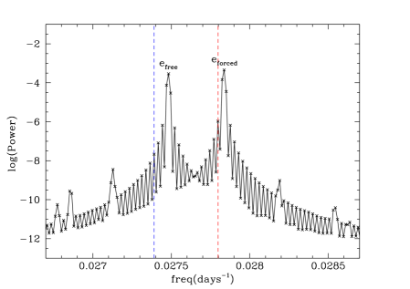
Figure 2: Power spectrum obtained from FFT of $R(t)/R_{0}$ for Kepler-16 b. See Table 1 for the parameter values. The vertical blue and red dashed lines indicate the analytic values of $\kappa_{0}$ and $n_{0}$, respectively, from the first-order epicyclic theory.

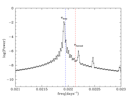
Figure 3: Same as Figure 2, but for Kepler-34 b.

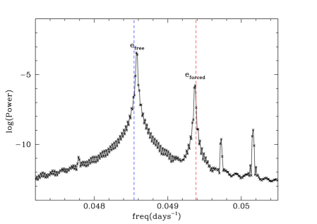
Figure 4: Same as Figure 2, but for Kepler-35 b.

Figures 2, 3, and 4 show the power spectra of the three exoplanets. We observe that two peaks corresponding to $e_{\rm free}$ and $e_{\rm forced}$ appear in the spectra at frequencies $\kappa_{0}$ and $n_{0}$ close to the analytic frequencies. Since the eccentricities of all three binary stars are non-zero, we expect $e_{\rm forced}$ to exist in all three spectra. For Kepler-16 b, its $e_{\rm free}$ and $e_{\rm forced}$ are comparable with each other. However, $e_{\rm forced}$ is $\sim 100$ times smaller than $e_{\rm free}$ in Kepler-34 b and $\sim 10$ times smaller than $e_{\rm free}$ in Kepler-35 b. According to Equation (38) of Leung & Lee (2013), which is the lowest order term in the expansion of the analytic expression for $e_{\rm forced}=C_{1}^{-}$ in powers of $a_{AB}/R_{0}$,

$$e_{\rm forced}\approx\frac{5}{4}e_{AB}\frac{m_{A}-m_{B}}{m_{A}+m_{B}}\frac{a_{AB}}{R_{0}}.$$ (5)

The reason for $e_{\rm forced}$ being small in the latter two systems is that the stars within each system are comparable to each other in mass, and $(m_{A}-m_{B})/(m_{A}+m_{B})$ is a small value. Even though $e_{AB}$ of Kepler-34 and Kepler-35 are 0.52068 and 0.14224, respectively, $e_{\rm forced}$ of Kepler-34 b and Kepler-35 b are significantly smaller than that of Kepler-16 b (see Table 1).

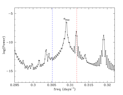
Figure 5: Power spectrum obtained from FFT of $R(t)/R_{0}$ for Styx. See Table 2 for the parameter values. The vertical blue and red dashed lines indicate the analytic values of $\kappa_{0}$ and $n_{0}$, respectively, from the first-order epicyclic theory.

Table 1 shows a comparison between the values obtained from the power spectra and those predicted by the first-order epicyclic theory of Leung & Lee (2013) for the three Kepler systems. The frequencies $n_{0}$ and $\kappa_{0}$ are shown in units of the Keplerian mean motion $n_{K}=[G(m_{A}+m_{B})/R_{0}^{3}]^{1/2}$ at $R_{0}$. The difference between the values of $e_{\rm forced}$ from the power spectra and the values from the epicyclic theory are $\sim 0.08\%$, $\sim 12\%$ and $\sim 3\%$ for Kepler-16 b, Kepler-34 b and Kepler-35 b, respectively. The large difference for Kepler-34 b is caused by the nature of the epicyclic theory, which is only accurate to first order in the binary eccentricity $e_{AB}$. If $e_{AB}$ is large, as in Kepler-34, where $e_{AB}=0.52068$, the analytic expressions of the epicyclic theory may not be accurate. For Kepler-16 and Kepler-35, $e_{AB}$ are only 0.16048 and 0.14224, respectively, which are more than 3 times smaller than $e_{AB}$ of Kepler-34. We should emphasize that the parameter values from the power spectra are more accurate than those from the analytic theory. This can be illustrated by the periapse precession period of Kepler-34 b, which is equal to $2\pi/|n_{0}-\kappa_{0}|$. The analytic periapse precession period is about 91 years, whereas the period calculated from the spectrum is 62.4 years, which agrees with the numerical result shown in the lower left panel of Figure 5 of Leung & Lee (2013).

Leung & Lee (2013) estimated the free parameter $e_{\rm free}$ from the variation of a transformed radius $R^{\prime}$, where the forced oscillation terms (including the forced eccentricity term) have been evaluated using the analytic expressions of the first-order epicyclic theory and subtracted from $R_{0}$. These are the values shown in parenthesis in Table 1. The more accurate values determined from the power spectra are smaller by $\sim 4$–$6$%.

In Figures 2 to 4, other than $e_{\rm free}$ and $e_{\rm forced}$ at $\kappa_{0}$ and $n_{0}$, we also observe peaks at frequencies which cannot be explained by the first-order epicyclic theory. We tested and confirmed the reality of these peaks by changing the output time steps and hence the resolution of the spectra, which does not change the peaks. The identity of these peaks is still unknown. We suspect that they may be due to higher order terms of $e_{AB}$ and forced oscillations, possibly with frequencies equal to some combinations of $n_{0}$ and $\kappa_{0}$. Further investigation is needed. There are also background fluctuations of the spectrum outside the peaks. We find that increasing the resolution of the spectrum decreases the amplitude of the background fluctuations and allows the peaks to look sharper. Hence, the background fluctuations are likely to be artifacts of FFT.

3.2 Satellites of Pluto-Charon

We also apply FFT to the satellites of Pluto-Charon. We perform simulations with the initial state vectors of the best fit of Showalter & Hamilton (2015), with a time step $\delta t$ of $3000\,$s. The output time step $\zeta$ is chosen to be 30 times $\delta t$ and the system is integrated for $\sim 1200$ days in order to generate high resolution spectra that can separate $n_{0}$ and $\kappa_{0}$.

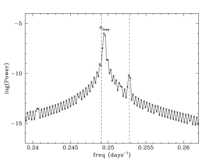
Figure 6: Same as Figure 5, but for Nix.

Figures 5 and 6 show the power spectra of Styx and Nix, respectively. We observe two peaks in the power spectra near the analytic values of $n_{0}$ and $\kappa_{0}$. The peak near $n_{0}$ is not expected, because the orbit of Pluto-Charon is circular ($e_{AB}=0$) and $e_{\rm forced}$ should be zero, according to the first-order epicyclic theory (see Equation (30) of Leung & Lee (2013) and Equation (5) above). This peak is likely due to higher order terms, but since we are not certain of its origin, we do not use the position of this peak to determine $n_{0}$ from the numerical integration. Instead, we use the cumulative increase in $\phi$, as in Lee & Peale (2006). The values of $\kappa_{0}$ and $e_{\rm free}$ are determined from the power spectrum.

Table 2 shows the numerical values of $n_{0}/n_{K}$, $\kappa_{0}/n_{K}$, and $e_{\rm free}$ for all four satellites. They are compared to the analytic values of $n_{0}/n_{K}$ and $\kappa_{0}/n_{K}$ from the first-order epicyclic theory and the best-fit values from Table 1 of Showalter & Hamilton (2015). The latter were obtained from an $8$-parameter fit of a precessing ellipse to the entire set of observational data, and we converted the apsidal precession rate $\dot{\varpi}$ to $\kappa_{0}$ using $\kappa_{0}=n_{0}-{\dot{\varpi}}$. For Nix, Kerberos, and Hydra, the values of $n_{0}/n_{K}$ and $\kappa_{0}/n_{K}$ by all three methods are in good agreement with each other, except that the analytic value of $\kappa_{0}/n_{K}$ is slightly smaller for Nix, and the values of $e_{\rm free}$ from the power spectrum are smaller than the eccentricity from the precessing ellipse fit by $\sim 3$–$9\%$. However, for Styx, the satellite closest to Pluto-Charon, the value of $\kappa_{0}/n_{K}$ from the power spectrum is significantly larger than the analytic and best-fit values (see also Figure 5), and the value of $e_{\rm free}$ is more than five times smaller than the best-fit value.

In addition to the $8$-parameter fit shown in their Table 1, where the nodal precession rate is derived from $n$ and $\dot{\varpi}$, Showalter & Hamilton (2015) also explored fits to the entire data set with $6$–$9$ parameters that make different assumptions about how the parameters are coupled, and the resulting orbiting elements are listed in their Extended Table 1. Interestingly, for Nix, Kerberos, and Hydra, all of the fits give similar results for $e$ and $\dot{\varpi}$ (and hence $\kappa_{0}$), but for Styx, the fits with $6$ and $7$ parameters give results that are different from those with $8$ and $9$ parameters. For $6$ and $7$ parameters, $e\approx 0.0011$, which is close to the value we find for $e_{\rm free}$ from the power spectrum, and ${\dot{\varpi}}=0.37688^{\circ}\,{\rm day}^{-1}$ or $\kappa_{0}/n_{K}\approx 0.9873$, which is larger than $\kappa_{0}/n_{K}\approx 0.9800$ for the $8$- and $9$-parameter fits but still smaller than $\kappa_{0}/n_{K}=0.99969$ from the power spectrum.

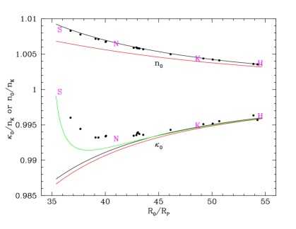
Figure 7: Mean motion $n_{0}$ and epicyclic frequency $\kappa_{0}$ in units of $n_{K}$ as a function of distance $R_{0}$ (in units of $R_{P}$) from the centre of mass of Pluto-Charon. Magenta alphabets and black dots show the numerical values from the power spectrum for the satellites Styx, Nix, Kerberos, and Hydra and the test particles from a simulation by Woo & Lee (2018) (see text for details). Black, red, and green curves are from the first-order epicyclic theory, the Hamiltonian theory with the secular term only, and the Hamiltonian theory with the secular and 3:1 mean-motion resonance terms, respectively.

To get a better understanding of this disagreement in the numerical and analytic values of $\kappa_{0}$ for Styx, we pick some test particles from our study of the early in-situ formation scenario of the small satellites (Woo & Lee, 2018) and apply FFT to their final orbits after the tidal evolution of Pluto-Charon. They are taken from the constant $\Delta t$ simulations shown in Figure 10 of Woo & Lee (2018), with the time lag of the tidal bulge of Pluto $\Delta t=600\,$s, the ratio of the rates of tidal dissipation in Charon and Pluto $A=40$, and the initial $e_{AB}=0$ (hence $e_{AB}=0$ from beginning to end), and they have small $e_{\rm free}$ ($\lesssim 10^{-4}$). Their $\kappa_{0}/n_{K}$ from the power spectrum and $n_{0}/n_{K}$ from the cumulative increase in $\phi$ are shown as black dots in Figure 7. The analytic expression from the first-order epicyclic theory (Equations (3) and (4)) are shown as black lines. As we can see, their $n_{0}$ and $\kappa_{0}$ follow the same trends as the actual satellites (magenta alphabets in Figure 7), with $n_{0}$ in good agreement with the analytic expression and $\kappa_{0}$ showing increasing deviation from the analytic expression as $R_{0}$ decreases. We shall seek an explanation for this deviation for $\kappa_{0}$ in Section 4.

3.3 Forced Oscillation Terms

Beside $e_{\rm free}$ and $e_{\rm forced}$, we also search for the peaks of the forced oscillation terms, which are located in higher frequency regions of the power spectrum, compared to $n_{0}$ and $\kappa_{0}$. Figure 8 shows the forced oscillation terms of Nix, and Figure 9 shows the forced oscillation terms of Kepler-16 b. More identifiable peaks are found in Figure 9 than in Figure 8, which can be explained by the epicyclic theory. From Equations (28) and (30) of Leung & Lee (2013), $C_{0}$ and $C_{k}^{\pm}$ are proportional to $e_{AB}$ and exist only when $e_{AB}$ is non-zero. Hence, we cannot find peaks of $C_{0}$, $C_{2}^{-}$ and $C_{3}^{-}$ in Figure 8 but they exist in Figure 9. We do not search for $C_{k}^{+}$ for Kepler-16 b, because their values are much smaller than the values of $C_{k}^{0}$ and $C_{k}^{-}$, for $k$ = 1 to 3 (see Table 2 of Leung & Lee 2013). There are many smaller peaks in Figures 8 and 9 at frequencies other than those associated with $C_{k}^{0}$, $C_{0}$ and $C_{k}^{\pm}$, whose identities are unknown but again could be due to higher order terms of $e_{AB}$ and forced oscillations.

We compare the amplitudes and frequencies of the forced oscillation terms from the power spectrum to their predicted values from the first-order epicyclic theory. The peaks are found at frequencies close to their analytic predictions. Table 3 shows the comparison between the amplitudes from the power spectrum and the analytic values from Leung & Lee (2013) for some of the forced oscillation terms of Kepler-16 b. We find that the amplitudes from the power spectrum are slightly lower than the analytic values. Similar to $e_{\rm forced}$, the slight difference is expected to be due to the inaccurate prediction from the first-order epicyclic theory of Leung & Lee (2013).

3.4 Uncertainties

The FFT results presented in the above subsections for each circumbinary object are obtained from a numerical orbit integration of the best fit using a specific time step. The uncertainties due to the numerical errors of the orbit integration can be estimated by varying the time step. In particular, we find that the uncertainty in $e_{\rm free}$ is less than $0.4\%$ for Styx and less than $0.05\%$ for the other satellites of Pluto-Charon. The uncertainties due to the uncertainties in the measurements can be determined by applying the FFT method to numerical orbit integrations of the distribution of fits from a Markov chain Monte Carlo or bootstrap analysis. Such an analysis is beyond the scope of the present paper.

4 MODIFICATION OF EPICYCLIC FREQUENCY BY 3:1 MEAN-MOTION RESONANCE

How can we explain the increasing deviation of $\kappa_{0}$ from the lowest order epicyclic theory at decreasing distance from the center of mass of Pluto-Charon seen in Figure 7? For motion around an oblate planet with $J_{2}$ and $J_{4}$, Borderies-Rappaport & Longaretti (1994) have extended the epicyclic theory to third order and found corrections to $n_{0}$, $\kappa_{0}$, and $\nu_{0}$ proportional to $e_{\rm free}^{2}$ and $i_{\rm free}^{2}$. Similar corrections from the axisymmetric components of the potential of a binary are negligible for the satellites and test particles shown in Figure 7, which have small $e_{\rm free}$ and $i_{\rm free}$. Generalizing this approach to account for the time varying non-axisymmetric components of the potential of a binary is difficult, with many forced oscillation terms to keep track of just to go from first order to second order.

Instead, we follow the Hamiltionian approach of Lithwick & Wu (2008). For a particle of mass $m$ orbiting a binary with primary mass $m_{A}$ and secondary mass $m_{B}$, the Hamiltonian in Jacobi coordinates is

$${\cal H}={\cal H}_{K,AB}+{\cal H}_{K}+{\cal H}_{\rm pert},$$ (6)

where

$${\cal H}_{K,AB}=-{Gm_{A}m_{B}\over 2a_{AB}}$$ (7)

represents the Keplerian motion of the binary with osculating semimajor axis $a_{AB}$,

$${\cal H}_{K}=-{G(m_{A}+m_{B})m\over 2a}$$ (8)

represents the Keplerian motion of the particle relative to the center of mass of the binary with osculating semimajor axis $a$, and

$${\cal H}_{\rm pert}=-Gmm_{A}\left({1\over{|\mbox{\boldmath$r$}-\mbox{\boldmath$r$}_{A}|}}-{1\over|\mbox{\boldmath$r$}|}\right)-Gmm_{B}\left({1\over{|\mbox{\boldmath$r$}-\mbox{\boldmath$r$}_{B}|}}-{1\over|\mbox{\boldmath$r$}|}\right)$$ (9)

represents the perturbations to the Keplerian motions (Lee & Peale, 2003). We shall consider the limit $m\ll m_{A}+m_{B}$, where the binary orbit is fixed.

In Equation (9), $r$, $\mbox{\boldmath$r$}_{A}=-m_{B}\mbox{\boldmath$r$}_{AB}/(m_{A}+m_{B})$, and $\mbox{\boldmath$r$}_{B}=m_{A}\mbox{\boldmath$r$}_{AB}/(m_{A}+m_{B})$ are the positions of the particle, primary, and secondary from the center of mass of the binary, respectively, where $\mbox{\boldmath$r$}_{AB}$ is the position of the secondary from the primary. For the terms $1/|\mbox{\boldmath$r$}-\mbox{\boldmath$r$}_{A}|$ and $1/|\mbox{\boldmath$r$}-\mbox{\boldmath$r$}_{B}|$, we can use the usual expansion of the direct part of the disturbing function $R_{D}=a/|\mbox{\boldmath$r$}-\mbox{\boldmath$r$}^{\prime}|$ for an outer body with $r>r^{\prime}$ into various terms given in, e.g., Chapter 6.5 of Murray & Dermott (1999). For the term $1/|\mbox{\boldmath$r$}|$, we can use the same expansion and take the limit $a^{\prime}/a\to 0$. If we assume that $e_{AB}=0$ and that the orbits are coplanar, we then find that

$${\cal H}_{\rm pert}={\cal H}_{\rm sec}+{\cal H}_{\rm 3:1}+\cdots,$$ (10)

where

$${\cal H}_{\rm sec} = -{Gmm_{A}\over a}\left[{1\over 2}b_{1/2}^{0}(\alpha)+{1\over 8}e^{2}(2\alpha D+\alpha^{2}D^{2})b_{1/2}^{0}(\alpha)-1\right]_{\alpha_{A}^{\prime}}$$ (11)

$$-{Gmm_{B}\over a}\left[{1\over 2}b_{1/2}^{0}(\alpha)+{1\over 8}e^{2}(2\alpha D+\alpha^{2}D^{2})b_{1/2}^{0}(\alpha)-1\right]_{\alpha_{B}^{\prime}}$$

is the secular term, and

$${\cal H}_{\rm 3:1} = +{Gmm_{A}\over a}\left[{1\over 8}e^{2}(17+10\alpha D+\alpha^{2}D^{2})b_{1/2}^{1}(\alpha)\right]_{\alpha_{A}^{\prime}}\cos(3\lambda-\lambda_{AB}-2\varpi)$$ (12)

$$-{Gmm_{B}\over a}\left[{1\over 8}e^{2}(17+10\alpha D+\alpha^{2}D^{2})b_{1/2}^{1}(\alpha)\right]_{\alpha_{B}^{\prime}}\cos(3\lambda-\lambda_{AB}-2\varpi)$$

is the 3:1 mean-motion resonance term. The expressions in the square brackets are evaluated at $\alpha=\alpha_{A}^{\prime}=a_{A}/a$ and $\alpha=\alpha_{B}^{\prime}=a_{B}/a$, $\lambda=n_{0}t+\psi_{0}$ and $\lambda_{AB}=n_{AB}t+\varphi_{AB}+\varpi_{B}$. Unlike Lithwick & Wu (2008), we do not expand the above expressions to leading order in $m_{B}/(m_{A}+m_{B})$.

From the equation of motion for $\lambda$,

$$n_{0}={d\lambda\over dt}={2\over m}\sqrt{a\over G(m_{A}+m_{B})}{\partial{\cal H}\over\partial a}$$ (13)

with the Keplerian and secular terms: ${\cal H}={\cal H}_{K}+{\cal H}_{\rm sec}$, we find that

$$n_{0} = \Bigg{\{}-1+{m_{A}\over(m_{A}+m_{B})}b_{1/2}^{0}(\alpha_{A}^{\prime})+{m_{B}\over(m_{A}+m_{B})}b_{1/2}^{0}(\alpha_{B}^{\prime})$$ (14)

$$\quad+{m_{A}m_{B}\over(m_{A}+m_{B})^{2}}\left(a_{AB}\over a\right)\left[Db_{1/2}^{0}(\alpha_{A}^{\prime})+Db_{1/2}^{0}(\alpha_{B}^{\prime})\right]$$

$$\quad+{1\over 8}{m_{A}m_{B}\over(m_{A}+m_{B})^{2}}\left(a_{AB}\over a\right)e^{2}\Big{[}4Db_{1/2}^{0}(\alpha_{A}^{\prime})+5\alpha_{A}^{\prime}D^{2}b_{1/2}^{0}(\alpha_{A}^{\prime})+\alpha_{A}^{\prime 3}D^{2}b_{1/2}^{0}(\alpha_{A}^{\prime})$$

$$\qquad+4Db_{1/2}^{0}(\alpha_{B}^{\prime})+5\alpha_{B}^{\prime}D^{2}b_{1/2}^{0}(\alpha_{B}^{\prime})+\alpha_{B}^{\prime 3}D^{2}b_{1/2}^{0}(\alpha_{B}^{\prime})\Big{]}\Bigg{\}}n_{a},$$

where $n_{a}=[G(m_{A}+m_{B})/a^{3}]^{1/2}$. The last term in Equation (14) is proportional to $e^{2}$, which is similar to the correction found by Borderies-Rappaport & Longaretti (1994) and can be neglected for the satellites of Pluto-Charon with small $e$. As Greenberg (1981) pointed out, if we consider only the axisymmetric components of the potential, a test particle on a circular orbit at $R_{0}$ is always at periapse in the osculating elements, i.e., $R_{0}=a_{\rm osc}(1-e_{\rm osc})$. We can then use the angular momentum of a circular orbit at $R_{0}$, $mR_{0}^{2}n_{0}=m\left[G(m_{A}+m_{B})a_{\rm osc}(1-e_{\rm osc}^{2})\right]^{1/2}$, to derive that $e_{\rm osc}=n_{0}^{2}/n_{K}^{2}-1$ and $a_{\rm osc}=R_{0}/(2-n_{0}^{2}/n_{K}^{2})$, where $n_{K}=[G(m_{A}+m_{B})/R_{0}^{3}]^{1/2}$ as before. Thus the appropriate expression to use for $a$ in Equation (14) is $a=R_{0}/(2-n_{0}^{2}/n_{K}^{2})$. This $n_{0}$ is plotted as the upper red curve in Figure 7, which is in good agreement with the upper black curve showing Equation (3) from the first-order epicyclic theory. It can also be shown analytically that Equations (3) and (14) (without the term proportional to $e^{2}$ in the latter) are equivalent to each other to the lowest order in the deviation of $n_{0}$ from $n_{K}$.

For the complex eccentricity $z=e\exp(i\varpi)$, the equation of motion (to the lowest order in $e$) is

$${dz\over dt}=-{2i\over m\sqrt{G(m_{A}+m_{B})a}}{\partial{\cal H}\over\partial z^{\ast}}$$ (15)

If we consider only the secular term ${\cal H}_{\rm sec}$,

$${dz\over dt}=i\eta z,$$ (16)

where

$$\eta = {1\over 4}{m_{A}m_{B}\over(m_{A}+m_{B})^{2}}\left(a_{AB}\over a\right)\Bigg{\{}2Db_{1/2}^{0}(\alpha_{A}^{\prime})+2Db_{1/2}^{0}(\alpha_{B}^{\prime})$$ (17)

$$\quad+\left(a_{AB}\over a\right)\left[{m_{A}\over(m_{A}+m_{B})}D^{2}b_{1/2}^{0}(\alpha_{B}^{\prime})+{m_{B}\over(m_{A}+m_{B})}D^{2}b_{1/2}^{0}(\alpha_{A}^{\prime})\right]\Bigg{\}}n_{a}.$$

The solution is

$$z=e_{\rm free}\exp(i\eta t).$$ (18)

So the secular periapse precession rate is ${\dot{\varpi}}=\eta$ and the epicyclic frequency is $\kappa_{0}=n_{0}-{\dot{\varpi}}=n_{0}-\eta$. This $\kappa_{0}$ is plotted as the lower red curve in Figure 7, using Equation (14) for $n_{0}$ and $a=R_{0}/(2-n_{0}^{2}/n_{K}^{2})$, and it is in good agreement with the lower black curve showing Equation (4) from the first-order epicyclic theory. Again it can be shown analytically that $\kappa_{0}$ from the first-order epicyclic theory and the secular Hamiltonian are equivalent to each other to the lowest order in the deviation of $\kappa_{0}$ from $n_{K}$.

Lithwick & Wu (2008) showed that the 3:1 mean-motion resonance term ${\cal H}_{\rm 3:1}$ can affect the rate of tidal damping even far from the nominal position of the resonance. Their derivation indicates that the 3:1 term can also affect the periapse precession rate. If we include the 3:1 resonance term ${\cal H}_{\rm 3:1}$ in the equation of motion for $z$,

$${dz\over dt}=i\eta z+i\nu z^{\ast}\exp\{i[(3n_{0}-n_{AB})t+\Delta\varphi]\},$$ (19)

where $\Delta\varphi=3\psi_{0}-\varphi_{AB}-\varpi_{B}$ and

$$\nu = {1\over 4}\Bigg{\{}{m_{B}\over(m_{A}+m_{B})}\left[17b_{1/2}^{1}(\alpha_{B}^{\prime})+10\alpha_{B}^{\prime}Db_{1/2}^{1}(\alpha_{B}^{\prime})+\alpha_{B}^{\prime 2}D^{2}b_{1/2}^{1}(\alpha_{B}^{\prime})\right]$$ (20)

$$\quad-{m_{A}\over(m_{A}+m_{B})}\left[17b_{1/2}^{1}(\alpha_{A}^{\prime})+10\alpha_{A}^{\prime}Db_{1/2}^{1}(\alpha_{A}^{\prime})+\alpha_{A}^{\prime 2}D^{2}b_{1/2}^{1}(\alpha_{A}^{\prime})\right]\Bigg{\}}n_{a}.$$

This equation has the solution $z=k\exp[i(\eta+b)t]+k(b/\nu)\exp[i(3n-n_{AB}-\eta-b)t+\Delta\varphi]$, where $b$ satisfies the quadratic equation

$$b^{2}-(3n-n_{AB}-2\eta)b+\nu^{2}=0,$$ (21)

which has the roots

$$b={(3n-n_{AB}-2\eta)\pm\sqrt{(3n-n_{AB}-2\eta)^{2}-4\nu^{2}}\over 2}.$$ (22)

The relevant root is the one with the positive sign. Hence

$$z=e_{\rm free}\exp[i(\eta+b)t]+e_{\rm free}(b/\nu)\exp\{i[(3n-n_{AB}-b-\eta)t+\Delta\varphi]\},$$ (23)

the periapse precession rate ${\dot{\varpi}}=\eta+b$, and the epicyclic frequency $\kappa_{0}=n_{0}-{\dot{\varpi}}=n_{0}-\eta-b$. This modified epicyclic frequency is plotted as the green curve in Figure 7. The effect of the 3:1 resonance is non-trivial even at the position of Nix near the nominal location of the 4:1 resonance, and it increases with decreasing distance to the nominal location of the 3:1 resonance. It explains a significant fraction of the discrepancy between the epicyclic frequencies from the power spectrum for the satellites and test particles and the epicyclic frequencies from the first-order epicyclic theory and the secular theory. The remaining discrepancy is likely due to other terms in the perturbation Hamiltonian that we have not considered.

5 SUMMARY AND DISCUSSION

In this paper, we have shown that the power spectrum generated by FFT of $R(t)/R_{0}$ from numerical orbit integration is a powerful tool for extracting the orbital parameters (such as $e_{\rm free}$, $e_{\rm forced}$, $\kappa_{0}$, $n_{0}$, etc.) of a circumbinary object. We applied this method to three Kepler circumbinary planets and the satellites of Pluto-Charon. The parameters extracted by the FFT power spectrum method are more accurate than the analytic values from the first-order epicyclic theory. This can be important in applications to circumbinary exoplanets where the binary eccentricity is large, as illustrated by the example of Kepler-34 b. This method is also able to determine accurately $e_{\rm free}$, which is a free parameter in the epicyclic theory.

The FFT method was used by Woo & Lee (2018) to measure $e_{\rm free}$ of test particles at the end of simulations of the early in-situ formation scenario of the small satellites of Pluto-Charon, which were compared to the eccentricities of the small satellites reported by Showalter & Hamilton (2015). In this paper, we have re-determined the orbital parameters of the small satellites by using the FFT method and found significant discrepancies in the values of $\kappa_{0}$ and $e_{\rm free}$ for Styx. The discrepancy in $\kappa_{0}$ means that the numerical value of the periapse precession rate ${\dot{\varpi}}=n_{0}-\kappa_{0}$ is only $41\%$ of the analytic value from the first-order epicyclic theory, while the numerical value of $e_{\rm free}$ is more than five times smaller than the eccentricity reported by Showalter & Hamilton (2015). By applying the FFT method to determine $\kappa_{0}$ for some test particles in the simulations of Woo & Lee (2018), we showed that there is a trend of increasing deviation of $\kappa_{0}$ from the analytic value of the first-order epicyclic theory as the distance from the center of mass of Pluto-Charon decreases. We have developed an analytic theory based on the disturbing function approach, which shows that this deviation in $\kappa_{0}$ is due to the modification of the secular precession frequency by the 3:1 mean-motion resonance.

The lower value of $e_{\rm free}$ for Styx also has implications for the origin and evolution of the satellites of Pluto-Charon. According to Table 1 of Showalter & Hamilton (2015), the eccentricity of Styx is similar to that of Hydra, while the eccentricity increases smoothly from Nix to Kerberos to Hydra (see also Table 2). Woo & Lee (2018) found that these eccentricities are similar to those of test particles that form in situ and survive to the end of the tidal evolution of Pluto-Charon in a model with constant tidal dissipation function $Q$, $Q_{P}=100$ for Pluto, the relative rate of tidal dissipation in Charon and Pluto $A=2.5$, and initial orbital eccentricity of Charon $e_{AB}=0.2$ (although this model does not explain the near resonance locations of the satellites). The revised, much lower $e_{\rm free}$ for Styx is no longer consistent with this model. It is unclear whether changes in $Q_{P}$, $A$ and/or initial $e_{AB}$ could result in eccentricities after tidal evolution that are consistent with the revised $e_{\rm free}$ of the satellites. Alternatively, it is interesting to note that the revised $e_{\rm free}$ increases smoothly from Styx to Hydra (see Table 2), which could be consistent with the cumulative effects of passing Kuiper belt objects on the orbits of the satellites (Collins & Sari, 2008). Further investigations into the viability of these scenarios are needed.

Table 1: Comparison of Parameter Values from Power Spectrum and Epicyclic Theory for Three Kepler Circumbinary Planets

Parameter	Numerical	Analytic
Kepler-16 b
$n_{K}$ (${\rm day}^{-1}$)	0.02760
$n_{0}/n_{K}$	1.00858	1.00702
$\kappa_{0}/n_{K}$	0.99574	0.99224
$e_{\rm free}$	0.0282	(0.030)
$e_{\rm forced}$	0.0358	0.0358
Kepler-34 b
$n_{K}$ (${\rm day}^{-1}$)	0.02204
$n_{0}/n_{K}$	1.00696	1.00423
$\kappa_{0}/n_{K}$	0.99445	0.99567
$e_{\rm free}$	0.193	(0.204)
$e_{\rm forced}$	0.00164	0.00186
Kepler-35 b
$n_{K}$ (${\rm day}^{-1}$)	0.04897
$n_{0}/n_{K}$	1.00825	1.00838
$\kappa_{0}/n_{K}$	0.99190	0.99119
$e_{\rm free}$	0.0364	(0.038)
$e_{\rm forced}$	0.00242	0.00249

Note. — The values of $e_{\rm free}$ in parenthesis were estimated from the variation of a transformed radius $R^{\prime}$ by Leung & Lee (2013) (see text for details).

Table 2: Comparison of Parameter Values from Power Spectrum, Epicyclic Theory, and Fit for Pluto-Charon Satellites

Parameter	Numerical	Analytic	Fit
Styx
$n_{K}$ (${\rm day}^{-1}$)	0.30898
$n_{0}/n_{K}$	1.00849	1.00903	1.00863
$\kappa_{0}/n_{K}$	0.99969	0.98770	0.98004
$e_{\rm free}$	0.00110	$\cdots$	0.00579
Nix
$n_{K}$ (${\rm day}^{-1}$)	0.25117
$n_{0}/n_{K}$	1.00650	1.00658	1.00649
$\kappa_{0}/n_{K}$	0.99306	0.99171	0.99377
$e_{\rm free}$	0.00187	$\cdots$	0.00204
Kerberos
$n_{K}$ (${\rm day}^{-1}$)	0.19445
$n_{0}/n_{K}$	1.00438	1.00452	1.00451
$\kappa_{0}/n_{K}$	0.99494	0.99468	0.99419
$e_{\rm free}$	0.00320	$\cdots$	0.00328
Hydra
$n_{K}$ (${\rm day}^{-1}$)	0.16389
$n_{0}/n_{K}$	1.00373	1.00354	1.00357
$\kappa_{0}/n_{K}$	0.99627	0.99598	0.99612
$e_{\rm free}$	0.00551	$\cdots$	0.00586

Table 3: Comparison of Values of Some Forced Oscillation Terms from Power Spectrum and Epicyclic Theory for Kepler-16 b

Parameter	Numerical	Analytic
$|C_{1}^{0}|$	0.000248	0.000282
$|C_{2}^{0}|$	0.000553	0.000589
$|C_{0}|$	0.000135	0.000159
$|C_{2}^{-}|$	0.002358	0.002438
$|C_{3}^{-}|$	0.000085	0.000110

Figure 8: Same as Figure 6, but with 2 times lower resolution and in a different frequency range showing the forced oscillation terms $|C_{1}^{0}|=0.00126$ at $|n_{0}-n_{AB}|=0.73091\,{\rm day}^{-1}$ and $|C_{2}^{0}|=0.00142$ at $2|n_{0}-n_{AB}|=1.46182\,{\rm day}^{-1}$.

Figure 9: Same as Figure 2, but with 2 times lower resolution and in a different frequency range showing the five forced oscillation terms $C_{1}^{0}$, $C_{2}^{0}$, $C_{0}$, $C_{2}^{-}$ and $C_{3}^{-}$. See Table 3 for the comparison between the values of the forced oscillation terms from the power spectrum and the first-order epicyclic theory.

References

- Borderies-Rappaport & Longaretti (1994) Borderies-Rappaport, N., & Longaretti, P.-Y. 1994, Icarus, 107, 129
- Brozović et al. (2015) Brozović, M., Showalter, M. R., Jacobson, R. A., & Buie, M. W. 2015, Icarus, 246, 317
- Collins & Sari (2008) Collins, B. F. & Sari, R. 2008, AJ, 136, 2552
- Doyle et al. (2011) Doyle, L. R., et al. 2012, Science, 333, 1602
- Greenberg (1981) Greenberg, R. 1981, AJ, 86, 912
- Kostov et al. (2016) Kostov, V. B., et al. 2016, ApJ, 827, 86
- Lee & Peale (2003) Lee, M. H., & Peale, S. J. 2003, ApJ, 592, 1201
- Lee & Peale (2006) Lee, M. H., & Peale, S. J. 2006, Icarus, 184, 573
- Leung & Lee (2013) Leung, G. C. K., & Lee, M. H. 2013, AJ, 763, 107
- Levison & Duncan (1994) Levison, H. F., & Duncan, M. J. 1994, Icarus, 108, 18
- Lithwick & Wu (2008) Lithwick, Y., & Wu, Y. 2008, preprint (arXiv:0802.2939)
- Murray & Dermott (1999) Murray, C. D., & Dermott, S. F. 1999, Solar System Dynamics (Cambridge: Cambridge Univ. Press)
- Press et al. (1992) Press, W. H., Teukolsky, S. A., Vetterling, W. T., & Flannery, B. P. 1992, Numerical Recipes in Fortran 77 (Cambridge: Cambridge Univ. Press)
- Showalter & Hamilton (2015) Showalter, M. R., & Hamilton, D. P. 2015, Nature, 522, 7554
- Welsh et al. (2012) Welsh, W. F., et al. 2012, Nature, 481, 475
- Wisdom & Holman (1991) Wisdom, J., & Holman, M. 1991, AJ, 102, 1528
- Woo & Lee (2018) Woo, M. Y., & Lee, M. H. 2018, AJ, 155, 175