TTP20-020, P3H-20-018

The Kinetic Heavy Quark Mass to Three Loops

Abstract

We compute three-loop corrections to the relation between the heavy quark masses defined in the pole and kinetic schemes. Using known relations between the pole and $\overline{\rm MS}$ quark masses we can establish precise relations between the kinetic and $\overline{\rm MS}$ charm and bottom masses. As compared to two loops, the precision is improved by a factor two to three. Our results constitute important ingredients for the precise determination of the Cabibbo-Kobayashi-Maskawa matrix element $|V_{cb}|$ at Belle II.

Introduction. Among the main aims of the Belle II experiment at the SuperKEKB accelerator at KEK (Tsukuba) is the precise measurement of various matrix elements in the Cabibbo-Kobayashi-Maskawa (CKM) mixing matrix. These are crucial ingredients for our understanding of charge-parity (CP) violation and indispensable input for precision tests of the Standard Model (SM) of particle physics. In this context the determination of $|V_{cb}|$, the CKM matrix element entering in $b\to c$ transitions, at the 1% level is of particular interest; at present its relative error of about 2% Amhis:2019ckw constitutes an important source of uncertainty in the predictions for $K\to\pi\nu\bar{\nu}$ Buras:1997fb ; Brod:2010hi , $B_{s}\to\mu^{+}\mu^{-}$ Bobeth:2013uxa and $\varepsilon_{K}$ Ligeti:2016qpi , the parameter which quantifies CP violation in kaon mixing. All such processes set strong constraints on new physics with a generic flavour and CP structure.

At present, the values of $|V_{cb}|$ from inclusive $b\to c\ell\nu$ decays are obtained from global fits of $|V_{cb}|$, the bottom and charm masses ($m_{b,c}$) and the relevant non-perturbative parameters in the heavy quark expansion. The most recent determination is $|V_{cb}|=(42.19\pm 0.78)\times 10^{-3}$ Gambino:2013rza ; Alberti:2014yda ; Gambino:2016jkc ; Amhis:2019ckw , where the precision is limited by perturbative and power correction uncertainties.

In analyses of $B\to X_{c}\ell\nu$ decays, it is mandatory to use a so-called “threshold” mass, designed such that the perturbative QCD corrections to the decay rate are well-behaved. So far, for the analyses either the kinetic mass ($m^{\rm kin}$) Bigi:1996si or the $1S$ mass Hoang:1999zc ; Hoang:1998hm ; Hoang:1998ng ; Bauer:2004ve have been chosen. Both schemes are well suited for $B\to X_{c}\ell\nu$, since they allow for renormalization scales $\mu\leq m_{b}$. The relation between the $1S$ and $\overline{\rm MS}$ quark mass ($\overline{m}$) has been computed up to next-to-next-to-next-to-leading order in Refs. Marquard:2015qpa ; Marquard:2016dcn . For the $m^{\rm kin}$–$\overline{m}$ relation two-loop corrections and the three-loop terms with two closed massless fermion loops (often referred to as large-$\beta_{0}$ terms) have been computed in Ref. Czarnecki:1997sz .

The rate and the moments of $B\to X_{c}\ell\nu$ strongly depend on the mass definition of the heavy quark, the choice of which is closely intertwined with the size of the QCD corrections. Perturbative calculations using the on-shell mass scheme are affected by the renormalon ambiguity, which manifests itself through bad behaviour of the perturbative series Beneke:1994sw ; Bigi:1994em . However, QCD corrections to the semi-leptonic rates exhibit a bad convergence also in the $\overline{\rm MS}$ scheme Bigi:1996si ; Melnikov:2000qh . In fact, large $(n\alpha_{s})^{k}$ terms, with $n=5$, arise from the $m^{\rm OS}$–$\overline{m}$ conversion of the overall factor $\Gamma\simeq G_{F}^{2}m_{b}^{5}|V_{cb}|^{2}/(192\pi^{3})$.

The kinetic scheme was introduced in Bigi:1996si to resum such $n$-enhanced terms via a suitable short-distance definition. It relies on the Small Velocity QCD sum rules Bigi:1994ga , which hold in the zero-recoil limit, i.e. for hadronic final state velocities $|\vec{v}\,|\ll 1$ in the rest frame of the decaying particle and $m_{b}\sim m_{c}$.

Note, that the semi-leptonic $B$ decays alone precisely determine only a linear combination of the heavy quark masses, approximately given by $m_{b}-0.8m_{c}$ Gambino:2013rza . Thus, in order to break the degeneracy one must include in the fit external constraints for the bottom and the charm masses, which are usually given in the $\overline{\rm MS}$ scheme. Until now the scheme-conversion uncertainty from $\overline{m}_{b}(\overline{m}_{b})$ to $m_{b}^{\rm kin}$(1GeV) dominates the uncertainty of the $\overline{\rm MS}$ bottom quark mass Gambino:2011cq . The global fits in Gambino:2013rza ; Alberti:2014yda employed only $\overline{m}_{c}$ as external input, as the gain in accuracy with the further inclusion of $\overline{m}_{b}$ would have been limited by scheme conversion Gambino:2013rza .

In this Letter we will present the complete three-loop corrections to the $\overline{m}$–$m^{\rm kin}$ relation, which lead to a significant improvement of the uncertainties in the mass conversion. Our results constitute a fundamental ingredient for future inclusion of ${\cal O}(\alpha_{s}^{3})$ corrections in semi-leptonic rates and spectral moments. Thus it is one of the major steps towards the reduction of the theoretical uncertainties affecting the $|V_{cb}|$ determination from inclusive decays at the 1% level or even below.

Kinetic mass definition. In Ref. Bigi:1996si (see also Ref. Czarnecki:1997sz ) the kinetic mass has been defined via its relation to the pole mass $m^{\rm OS}$ through

$$m^{\rm kin}(\mu) = m^{\rm OS}-\overline{\Lambda}(\mu)|_{\rm pert}-\frac{\mu_{\pi}^{2}(\mu)|_{\rm pert}}{2m^{\rm kin}}+\ldots\,,$$ (1)

where the ellipses stand for contributions from higher dimensional operators. The scale $\mu$, the so-called Wilsonian cut-off, is part of the definition of $m^{\rm kin}$ and takes the role of a normalization point for the kinetic mass. In practice it is of the order of 1 GeV.

The quantities $\overline{\Lambda}(\mu)|_{\rm pert}$ and $\mu_{\pi}^{2}(\mu)|_{\rm pert}$ in Eq. (1) correspond to the heavy meson’s binding energy and the residual kinetic energy parameters, respectively. They are defined within perturbation theory and are obtained from the forward scattering amplitude of an external current $J$ and the heavy quark $Q$ [cf. Fig. 1(a)]

$$T(q_{0},\vec{q}\,) = \frac{i}{2m}\int{\rm d}^{4}{x\,}e^{-iqx}\langle Q|TJ(x)J^{\dagger}(0)|Q\rangle\,,$$ (2)

where for later convenience we have separated the energy and three-momentum components of the external momentum $q$. We furthermore denote the external momentum of the heavy quark by $p$ with $p^{2}=m^{2}$, and we introduce $s=(p+q)^{2}$. We assume that the current $J$ does not change the flavour of the heavy quark with mass $m$. For $\overline{\Lambda}(\mu)|_{\rm pert}$ and $\mu_{\pi}^{2}(\mu)|_{\rm pert}$ one has in the rest frame of the heavy quark Bigi:1996si ; Czarnecki:1997sz

$$\overline{\Lambda}(\mu)|_{\rm pert} = \lim_{\vec{v}\to 0}\lim_{m\to\infty}\frac{2}{\vec{v}\,^{2}}\frac{\int_{0}^{\mu}\omega W(\omega,\vec{v}\,){\rm d}\omega}{\int_{0}^{\mu}W(\omega,\vec{v}\,){\rm d}\omega}\,,$$

$$\mu_{\pi}^{2}(\mu)|_{\rm pert} = \lim_{\vec{v}\to 0}\lim_{m\to\infty}\frac{3}{\vec{v}\,^{2}}\frac{\int_{0}^{\mu}\omega^{2}W(\omega,\vec{v}\,){\rm d}\omega}{\int_{0}^{\mu}W(\omega,\vec{v}\,){\rm d}\omega}\,,$$ (3)

where the structure function $W$ is given by the discontinuity of $T$, $W=2\mbox{Im}\left[T(q_{0},\vec{q}\,)\right]$. In Eq. (3) we have $\omega=q_{0}-q_{0}^{\rm min}$, $\vec{v}=\vec{q}/m$ and $q_{0}^{\rm min}=\sqrt{\vec{q}\,^{2}+m^{2}}-m=mv^{2}/2+{\cal O}(v^{4})$. Note that $W$ is zero for $q_{0}<q_{0}^{\rm min}$.

In order to compute corrections of ${\cal O}(\alpha_{s}^{3})$ to Eq. (1) one has to consider three-loop corrections to the imaginary part of $T(q_{0},\vec{q}\,)$ in Eq. (2). This requires the evaluation of real and virtual corrections to the scattering process shown schematically in Fig. 1(a).

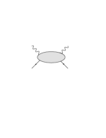
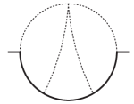
(a)	(b)

Figure 1: (a) Schematic Feynman diagram representing the scattering of an external current, represented by wavy lines and a heavy quark (solid line). The blob represents one-particle irreducible quantum corrections, which we consider up to three-loop order. (b) The most complicated master integral. Dotted lines represent massless relativistic propagators and solid lines stand for eikonal propagators with mass $y$.

More details on the derivation of Eq. (3) are provided in Ref. Fael_etal .

Calculation. From Eqs. (1) and (3) we learn that the relation between the kinetic and pole mass is obtained from the imaginary part of the structure function $W(\omega,\vec{v}\,)$ in the limit $\vec{v}\to 0$. It is thus suggestive to apply the threshold expansion Beneke:1997zp ; Smirnov:2012gma , which in our situation reduces to two momentum regions: the loop momenta can be either hard (h) and scale as the quark mass $m$, or ultra-soft (u) and scale as $y/m$ where $y=m^{2}-s$ measures the distance to the threshold. Note that in our case we have $y<0$. When expanding the denominators one has to assume that both $p$ and $q$ scale as $m$.

We generate the four-point Feynman amplitudes with qgraf Nogueira:1991ex and translate the output to FORM Ruijl:2017dtg notation. We make sure that the external momenta $p$ and $q$ are routed through the heavy quark line. Afterwards we expand all loop momenta according to the rules of asymptotic expansion which leads to a decomposition of each integral into regions in which the individual loop momenta either scale as hard or ultra-soft. At one-loop order there are only two regions. At two loops we have the regions (uu), (uh) and (hh), and at three loops we have (uuu), (uuh), (uhh) and (hhh). For each diagram we have cross-checked the scaling of the loop momenta using the program asy Pak:2010pt . Note that the contributions where all loop momenta are hard can be discarded since there are no imaginary parts. The mixed regions are expected to cancel after renormalization and decoupling of the heavy quark from the running of the strong coupling constant. Nevertheless we perform an explicit calculation of the (uh), (uuh) and (uhh) regions and use the cancellation as cross check. The physical result for the quark mass relation is solely provided by the purely ultra-soft contributions.

The starting point of our calculation are four-point functions. However, after the various expansions we obtain two-point functions with external momentum $p$. As a consequence denominators become linearly dependent and a partial fraction decomposition is needed in order to generate linear independent sets of propagators. They serve as input for FIRE Smirnov:2019qkx and LiteRed Lee:2012cn which are used for the reduction to master integrals.

After partial fraction decomposition we end up with 1, 2 and 14 pure ultra-soft integral families at one-, two- and three-loop order, respectively. The three-loop families have eight propagators and four irreducible numerators, three of which contain scalar products of the loop momenta and the external momentum $q$ and have been introduced to avoid an expensive tensor reduction.

After reduction to master integrals and their subsequent minimization across all families the amplitude can be expressed in terms of 1, 3 and 20 ultra-soft master integrals at one-, two- and three-loop order, respectively. At one and two loops all of them can be expressed in terms of $\Gamma$ functions. This is also the case for 11 of the three-loop master integrals. For 8 of the remaining integrals we obtain analytic results for the $\epsilon$ expansion with the help of Mellin-Barnes Smirnov:2012gma representations. In these cases the residues obtained after closing the integration contour can be summed analytically with the packages Sigma Schneider:2007 , EvaluateMultiSums Ablinger:2010pb together with HarmonicSums HarmonicSums ; additionally we obtain high-precision numerical results and use the PSLQ PSLQ algorithm to reconstruct the analytic expression. We have only encountered one integral where a different strategy was necessary. It is shown in graphical form in Fig. 1(b). For this integral we have introduced a different mass scale, $x$, in the bottom-middle propagator. In case this mass is zero ($x=0$), the integral can be computed analytically. Thus, it is suggestive to establish differential equations Kotikov:1990kg ; Gehrmann:1999as ; Henn:2013pwa , apply boundary conditions at $x=0$, and evaluate the solution for $x=1$, which provides the desired integral. We will provide more details on the computation of the master integrals in Ref. Fael_etal .

Let us mention that we have performed our calculation for a general gauge parameter $\xi$. We expand the amplitude up to linear order in $\xi$ and check that $\xi$ cancels after adding the quark mass counterterms. Furthermore, for the external current $J$ we use both a vector ($J=\bar{Q}\gamma_{\mu}Q$) and a scalar ($J=\bar{Q}Q$) current and check that the final result for the relation between the pole and kinetic mass is the same. However, the intermediate expressions are different. This concerns, e.g., the renormalization of the current itself. Whereas the vector current has a vanishing anomalous dimension an explicit renormalization constant is needed for the scalar current. Furthermore, in the case of the vector current there is no contribution from the virtual corrections contained in the denominator of Eq. (3) since in the static limit the Dirac form factor vanishes and the Pauli form factor is suppressed by $q^{2}$. On the other hand, in the scalar case there is a contribution from the finite static form factor.

Results. The main result of our calculation is the relation between the kinetic and the pole mass, which up to order $\alpha_{s}^{3}$ is given by

$$\frac{m^{\text{kin}}}{m^{\text{OS}}} = 1-\frac{\alpha_{s}^{(n_{l})}}{\pi}C_{F}\biggl{(}\frac{4}{3}\frac{\mu}{m^{\text{OS}}}+\frac{1}{2}\frac{\mu^{2}}{\left({m^{\text{OS}}}\right)^{2}}\biggr{)}+\left(\frac{\alpha_{s}^{(n_{l})}}{\pi}\right)^{2}C_{F}\Biggl{\{}\frac{\mu}{{m^{\text{OS}}}}\Biggl{[}C_{A}\biggl{(}-\frac{215}{27}+\frac{2\pi^{2}}{9}+\frac{22}{9}l_{\mu}\biggr{)}+n_{l}T_{F}\biggl{(}\frac{64}{27}-\frac{8}{9}l_{\mu}\biggr{)}\Biggr{]}$$ (4)

$$\mbox{}+\frac{\mu^{2}}{\left({m^{\text{OS}}}\right)^{2}}\Biggl{[}C_{A}\biggl{(}-\frac{91}{36}+\frac{\pi^{2}}{12}+\frac{11}{12}l_{\mu}\biggr{)}+n_{l}T_{F}\biggl{(}\frac{13}{18}-\frac{1}{3}l_{\mu}\biggr{)}\Biggr{]}\Biggr{\}}+\left(\frac{\alpha_{s}^{(n_{l})}}{\pi}\right)^{3}C_{F}\Biggl{\{}\frac{\mu}{{m^{\text{OS}}}}\Biggl{[}C_{A}^{2}\biggl{(}-\frac{130867}{1944}$$

$$\mbox{}+\frac{511\pi^{2}}{162}+\frac{19\zeta_{3}}{2}-\frac{\pi^{4}}{18}+\biggl{(}\frac{2518}{81}-\frac{22\pi^{2}}{27}\biggr{)}l_{\mu}-\frac{121}{27}l_{\mu}^{2}\biggr{)}+C_{A}n_{l}T_{F}\biggl{(}\frac{19453}{486}-\frac{104\pi^{2}}{81}-2\zeta_{3}$$

$$\mbox{}+\biggl{(}-\frac{1654}{81}+\frac{8\pi^{2}}{27}\biggr{)}l_{\mu}+\frac{88}{27}l_{\mu}^{2}\biggr{)}+C_{F}n_{l}T_{F}\biggl{(}\frac{11}{4}-\frac{4\zeta_{3}}{3}-\frac{2}{3}l_{\mu}\biggr{)}+n_{l}^{2}T_{F}^{2}\biggl{(}-\frac{1292}{243}+\frac{8\pi^{2}}{81}+\frac{256}{81}l_{\mu}-\frac{16}{27}l_{\mu}^{2}\biggr{)}\Biggr{]}$$

$$\mbox{}+\frac{\mu^{2}}{\left({m^{\text{OS}}}\right)^{2}}\Biggl{[}C_{A}^{2}\biggl{(}-\frac{96295}{5184}+\frac{445\pi^{2}}{432}+\frac{57\zeta_{3}}{16}-\frac{\pi^{4}}{48}+\biggl{(}\frac{2155}{216}-\frac{11\pi^{2}}{36}\biggr{)}l_{\mu}-\frac{121}{72}l_{\mu}^{2}\biggr{)}+C_{A}n_{l}T_{F}\biggl{(}\frac{13699}{1296}-\frac{23\pi^{2}}{54}$$

$$\mbox{}-\frac{3\zeta_{3}}{4}+\biggl{(}-\frac{695}{108}+\frac{\pi^{2}}{9}\biggr{)}l_{\mu}+\frac{11}{9}l_{\mu}^{2}\biggr{)}+C_{F}n_{l}T_{F}\biggl{(}\frac{29}{32}-\frac{\zeta_{3}}{2}-\frac{1}{4}l_{\mu}\biggr{)}+n_{l}^{2}T_{F}^{2}\biggl{(}-\frac{209}{162}+\frac{\pi^{2}}{27}+\frac{26}{27}l_{\mu}-\frac{2}{9}l_{\mu}^{2}\biggr{)}\Biggr{]}\Biggr{\}}\,,$$

where $l_{\mu}=\ln\frac{2\mu}{\mu_{s}}$, $\mu$ denotes the Wilsonian cut-off and $\mu_{s}$ is the renormalization scale of the strong coupling constant. The colour factors of the SU$(N_{C})$ gauge group are given by $C_{F}=(N_{C}^{2}-1)/(2N_{C})$, $C_{A}=N_{C}$ and $T_{F}=1/2$ and the strong coupling constant is defined in the $n_{l}$ flavour theory, where $n_{l}$ denotes the number of light quark fields. Note that in our calculation no effects of finite charm quark masses are taken into account. The two-loop result of Eq. (4) and the $n_{l}^{2}$ term at three loops agree with Ref. Czarnecki:1997sz .

Next we replace the pole mass on the r.h.s. of Eq. (4) by the $\overline{\rm MS}$ mass using results up to three loops Chetyrkin:1999ys ; Chetyrkin:1999qi ; Melnikov:2000qh . Also here we use $\alpha_{s}^{(n_{l})}$ as the expansion parameter. In order to obtain compact expressions we identify the renormalization scales of the $\overline{\rm MS}$ parameters $\alpha_{s}$ and $\overline{m}$ and furthermore specify the colour factors to QCD ($N_{C}=3$). This leads to

$$\frac{m^{\text{kin}}}{\overline{m}} = 1+\frac{\alpha_{s}^{(n_{l})}}{\pi}\biggl{(}\frac{4}{3}+l_{m}-\frac{16}{9}\frac{\mu}{\overline{m}}-\frac{2}{3}\frac{\mu^{2}}{\overline{m}^{2}}\biggr{)}+\left(\frac{\alpha_{s}^{(n_{l})}}{\pi}\right)^{2}\Biggl{\{}\frac{307}{32}+\frac{\pi^{2}}{3}-\frac{\zeta_{3}}{6}+\frac{\pi^{2}}{9}l_{2}+\frac{509}{72}l_{m}+\frac{47}{24}l_{m}^{2}-n_{l}\biggl{(}\frac{71}{144}+\frac{\pi^{2}}{18}$$ (5)

$$\mbox{}+\frac{13}{36}l_{m}+\frac{1}{12}l_{m}^{2}\biggr{)}+\frac{\mu}{\overline{m}}\biggl{[}-\frac{860}{27}+\frac{8\pi^{2}}{9}+\frac{88}{9}l_{\mu}+n_{l}\biggl{(}\frac{128}{81}-\frac{16}{27}l_{\mu}\biggr{)}\biggr{]}+\frac{\mu^{2}}{\overline{m}^{2}}\biggl{[}-\frac{83}{9}+\frac{\pi^{2}}{3}+\frac{2}{3}l_{m}+\frac{11}{3}l_{\mu}$$

$$\mbox{}+n_{l}\biggl{(}\frac{13}{27}-\frac{2}{9}l_{\mu}\biggr{)}\biggr{]}\Biggr{\}}+\left(\frac{\alpha_{s}^{(n_{l})}}{\pi}\right)^{3}\Biggl{\{}\frac{8462917}{93312}+\frac{652841\pi^{2}}{38880}+\frac{58\zeta_{3}}{27}-\frac{695\pi^{4}}{7776}-\frac{220a_{4}}{27}-\frac{1439\pi^{2}\zeta_{3}}{432}+\frac{1975\zeta_{5}}{216}$$

$$\mbox{}-\frac{575\pi^{2}}{162}l_{2}-\frac{22\pi^{2}}{81}l_{2}^{2}-\frac{55}{162}l_{2}^{4}+l_{m}\biggl{(}\frac{93391}{1296}+\frac{13\pi^{2}}{6}-\frac{23\zeta_{3}}{12}+\frac{13\pi^{2}}{18}l_{2}\biggr{)}+\frac{21715}{864}l_{m}^{2}+\frac{1861}{432}l_{m}^{3}+n_{l}\biggl{[}-\frac{231847}{23328}$$

$$\mbox{}-\frac{991\pi^{2}}{648}-\frac{241\zeta_{3}}{72}+\frac{61\pi^{4}}{1944}+\frac{8a_{4}}{27}-\frac{11\pi^{2}}{81}l_{2}+\frac{2\pi^{2}}{81}l_{2}^{2}+\frac{1}{81}l_{2}^{4}-l_{m}\biggl{(}\frac{5171}{648}+\frac{17\pi^{2}}{36}+\frac{7\zeta_{3}}{9}+\frac{\pi^{2}}{27}l_{2}\biggr{)}-\frac{385}{144}l_{m}^{2}$$

$$\mbox{}-\frac{43}{108}l_{m}^{3}\biggr{]}+n_{l}^{2}\biggl{[}\frac{2353}{23328}+\frac{13\pi^{2}}{324}+\frac{7\zeta_{3}}{54}+l_{m}\biggl{(}\frac{89}{648}+\frac{\pi^{2}}{54}\biggr{)}+\frac{13}{216}l_{m}^{2}+\frac{1}{108}l_{m}^{3}\biggr{]}+\frac{\mu}{\overline{m}}\biggl{[}-\frac{130867}{162}+\frac{1022\pi^{2}}{27}$$

$$\mbox{}+114\zeta_{3}-\frac{2\pi^{4}}{3}+l_{\mu}\biggl{(}\frac{10072}{27}-\frac{88\pi^{2}}{9}\biggr{)}-\frac{484}{9}l_{\mu}^{2}+n_{l}\biggl{(}\frac{20047}{243}-\frac{208\pi^{2}}{81}-\frac{140\zeta_{3}}{27}+l_{\mu}\biggl{(}-\frac{3356}{81}+\frac{16\pi^{2}}{27}\biggr{)}$$

$$\mbox{}+\frac{176}{27}l_{\mu}^{2}\biggr{)}+n_{l}^{2}\biggl{(}-\frac{1292}{729}+\frac{8\pi^{2}}{243}+\frac{256}{243}l_{\mu}-\frac{16}{81}l_{\mu}^{2}\biggr{)}\biggr{]}+\frac{\mu^{2}}{\overline{m}^{2}}\biggl{[}-\frac{22055}{108}+\frac{437\pi^{2}}{36}+\frac{1535\zeta_{3}}{36}-\frac{\pi^{4}}{4}+\frac{2\pi^{2}}{27}l_{2}$$

$$\mbox{}+l_{m}\biggl{(}\frac{1409}{108}-\frac{\pi^{2}}{3}\biggr{)}+l_{\mu}\biggl{(}\frac{689}{6}-\frac{11\pi^{2}}{3}\biggr{)}-\frac{11}{3}l_{m}l_{\mu}+\frac{23}{36}l_{m}^{2}-\frac{121}{6}l_{\mu}^{2}+n_{l}\biggl{(}\frac{1699}{81}-\frac{8\pi^{2}}{9}-\frac{35\zeta_{3}}{18}-\frac{13}{18}l_{m}$$

$$\mbox{}+l_{\mu}\biggl{(}-\frac{691}{54}+\frac{2\pi^{2}}{9}\biggr{)}+\frac{2}{9}l_{m}l_{\mu}-\frac{1}{18}l_{m}^{2}+\frac{22}{9}l_{\mu}^{2}\biggr{)}+n_{l}^{2}\biggl{(}-\frac{209}{486}+\frac{\pi^{2}}{81}+\frac{26}{81}l_{\mu}-\frac{2}{27}l_{\mu}^{2}\biggr{)}\biggr{]}\Biggr{\}}\,,$$

with $\overline{m}=\overline{m}(\mu_{s})$ and

$$l_{m}=\ln\frac{\mu_{s}^{2}}{\overline{m}^{2}},\,l_{2}=\ln 2,\,a_{4}=\text{Li}_{4}\left(\frac{1}{2}\right)\,.$$ (6)

We are now in the position to specify our results to the charm and bottom quark systems and check the perturbative stability of the quark mass relations.

The input values for our numerical analysis are $\alpha_{s}^{(5)}(M_{Z})=0.1179$ Tanabashi:2018oca , $\overline{m}_{c}(3~{}\mbox{GeV})=0.993$ GeV Chetyrkin:2017lif and $\overline{m}_{b}(\overline{m}_{b})=4.163$ GeV Chetyrkin:2009fv . We use RunDec Herren:2017osy for the running of the $\overline{\rm MS}$ parameters and the decoupling of heavy particles. For the Wilsonian cut-off we choose $\mu=1$ GeV for bottom Gambino:2013rza and $\mu=0.5$ GeV for charm Gambino:2010jz .

Let us start with the charm quark where we have $n_{l}=3$. We aim for a relation between $m_{c}^{\rm kin}$ and $\overline{m}_{c}(\mu_{s})$ for different choices of $\mu_{s}$. Often numerical values for $\overline{m}_{c}(\overline{m}_{c})$ are provided. However, this choice suffers from small renormalization scales of the order 1 GeV. A more appropriate choice is thus $\overline{m}_{c}(2~{}\mbox{GeV})$ or $\overline{m}_{c}(3~{}\mbox{GeV})$. For the three choices we obtain the following perturbative expansions

$$m_{c}^{\rm kin} = \hphantom{0}993+191+100+52~{}\mbox{MeV}=1336~{}\mbox{MeV}\,,$$

$$m_{c}^{\rm kin} = 1099+163+\hphantom{0}76+34~{}\mbox{MeV}=1372~{}\mbox{MeV}\,,$$

$$m_{c}^{\rm kin} = 1279+\hphantom{0}{84}+\hphantom{0}{30}+11~{}\mbox{MeV}=1404~{}\mbox{MeV}\,,$$ (7)

where from top to bottom $\mu_{s}=3~{}\mbox{GeV},2~{}\mbox{GeV}$ and $\overline{m}_{c}$ have been chosen. Within each equation the four numbers after the first equality sign refer to the tree-level results and the one-, two- and three-loop corrections. One observes that for each choice of $\mu_{s}$ the perturbative expansion behaves reasonably. The three-loop terms range from $11$ MeV to $52$ MeV and roughly cover the splitting of the final numbers for $m_{c}^{\rm kin}(0.5~{}\mbox{GeV})$.

In the case of the bottom quark we follow Ref. Gambino:2011cq and adapt two different schemes for the charm quark: we either consider the charm quark as decoupled and set $n_{l}=3$, or we set $n_{l}=4$ which corresponds to $m_{c}=0$. (In the latter case one could include $m_{c}/m_{b}$ corrections which we postpone to a future analysis Fael_etal .)

Using $\overline{m}_{b}(\overline{m}_{b})$ as input we obtain the following results for the kinetic mass

$$m_{b}^{\rm kin} = 4163+248+81+30~{}\mbox{MeV}=4521~{}\mbox{MeV}\,,$$

$$m_{b}^{\rm kin} = 4163+259+77+25~{}\mbox{MeV}=4523~{}\mbox{MeV}\,,$$ (8)

where the top and bottom line correspond to $n_{l}=3$ and $n_{l}=4$, respectively. In both cases we observe a good convergence of the perturbative series: the coefficients reduce by factors between $\approx 2.5$ and $\approx 3.5$ when including higher orders. We suggest to estimate the unknown four-loop corrections and contributions from higher dimensional operators, which scale as $\alpha_{s}\mu^{3}/m_{b}^{3}\sim\alpha_{s}^{4}$, by 50% of the three-loop corrections and assign an uncertainty of $15$ MeV and $12$ MeV for $n_{l}=3$ and $n_{l}=4$, respectively. Note, that our $\overline{m}_{b}$–$m_{b}^{\rm kin}$ scheme-conversion uncertainties are now smaller than the error of $m_{b}^{\rm kin}$ as determined by global fits: $m_{b}^{\rm kin}(1~{}\mbox{GeV})=4554\pm 18$ MeV Amhis:2019ckw .

For the computation of $\overline{m}_{b}(\overline{m}_{b})$ from the kinetic mass we proceed as follows: we first use the inverted version of Eq. (5) to compute the $\overline{\rm MS}$ bottom quark mass at the scale $\mu_{s}=m_{b}^{\rm kin}$. Afterwards, we use the QCD renormalization group equations at five-loop accuracy Baikov:2014qja ; Luthe:2016xec ; Baikov:2017ujl ; Baikov:2016tgj ; Herzog:2017ohr ; Luthe:2017ttg ; Chetyrkin:2017bjc as implemented in RunDec Herren:2017osy to run to $\mu_{s}=\overline{m}_{b}$. In order to demonstrate the perturbative series we choose $m_{b}^{\rm kin}$ from Eq. (8) and obtain for $n_{l}=3$ and $n_{l}=4$

$$\overline{m}_{b}(m_{b}^{\rm kin}) = 4521-273-101-39~{}\mbox{MeV}\,,$$

$$\overline{m}_{b}(m_{b}^{\rm kin}) = 4523-286-\hphantom{0}98-34~{}\mbox{MeV}\,,$$ (9)

with similar convergence properties as in Eq. (8). Thus we estimate the uncertainty from unknown higher order corrections as $\pm 18$ MeV and $\pm 17$ MeV, respectively. In an alternative approach one can estimate the uncertainty from the variation of the intermediate scale $\mu_{s}$ which leads to similar uncertainty estimates.

Finally, we present simple formulae which can be used to convert the scale-invariant bottom quark mass to the kinetic scheme or vice versa using the preferred input values for the mass and strong coupling constant. We have

$$\frac{\overline{m}_{b}(\overline{m}_{b})}{\mbox{MeV}} = 4163+\Delta^{(n_{l})}_{\rm kin}\{13,13\}-\Delta_{\alpha_{s}}\{7,7\}\pm\{18,17\}\,,$$

$$\frac{m_{b}^{\rm kin}}{\mbox{MeV}} = 4522+\Delta_{\overline{\rm MS}}\{18,18\}+\Delta_{\alpha_{s}}\{8,8\}\pm\{15,12\}\,,$$

where the first (second) number in the curly brackets corresponds to $n_{l}=3$ ($n_{l}=4$). Furthermore, we have defined $\Delta^{(3)}_{\rm kin}=(m_{b}^{\rm kin}/\mbox{MeV}-4518)/15$, $\Delta^{(4)}_{\rm kin}=(m_{b}^{\rm kin}/\mbox{MeV}-4520)/15$, $\Delta_{\overline{\rm MS}}=(\overline{m}_{b}(\overline{m}_{b})/\mbox{MeV}-4163)/16$ and $\Delta_{\alpha_{s}}=(\alpha_{s}-0.1179)/0.001$.

Conclusions. The main purpose of this Letter is the improvement of the precision in the conversion relation between the heavy quark kinetic and $\overline{\rm MS}$ masses. This goal is reached by computing the relation between the kinetic and pole mass to three-loop order; previously only two-loop corrections, supplemented by large-$\beta_{0}$ terms, were available. The main results of this paper can be found in Eqs. (4) and (5). Using a conservative uncertainty estimate the new corrections reduces the uncertainty in transformation formulas by about a factor two. Our findings constitute important ingredients in the extraction of $|V_{cb}|$ at the percent level or even below.

Acknowledgements. We thank Andrzej Czarnecki and Mikołaj Misiak for useful discussions and communications and Alexander Smirnov for help in the use of asy Pak:2010pt . We also thank Joshua Davies and Thomas Mannel for carefully reading the manuscript. We are grateful to Florian Herren for providing us his program which automates the partial fraction decomposition in case of linearly dependent denominators. This research was supported by the Deutsche Forschungsgemeinschaft (DFG, German Research Foundation) under grant 396021762 — TRR 257 “Particle Physics Phenomenology after the Higgs Discovery”.

References

- (1) Y. S. Amhis et al. [HFLAV], [arXiv:1909.12524 [hep-ex]].
- (2) A. J. Buras and R. Fleischer, Adv. Ser. Direct. High Energy Phys. 15 (1998), 65-238 [arXiv:hep-ph/9704376 [hep-ph]].
- (3) J. Brod, M. Gorbahn and E. Stamou, Phys. Rev. D 83 (2011), 034030 [arXiv:1009.0947 [hep-ph]].
- (4) C. Bobeth, M. Gorbahn, T. Hermann, M. Misiak, E. Stamou and M. Steinhauser, Phys. Rev. Lett. 112 (2014), 101801 [arXiv:1311.0903 [hep-ph]].
- (5) Z. Ligeti and F. Sala, JHEP 09 (2016), 083 [arXiv:1602.08494 [hep-ph]].
- (6) P. Gambino and C. Schwanda, Phys. Rev. D 89 (2014) no.1, 014022 [arXiv:1307.4551 [hep-ph]].
- (7) A. Alberti, P. Gambino, K. J. Healey and S. Nandi, Phys. Rev. Lett. 114 (2015) no.6, 061802 [arXiv:1411.6560 [hep-ph]].
- (8) P. Gambino, K. J. Healey and S. Turczyk, Phys. Lett. B 763 (2016), 60-65 [arXiv:1606.06174 [hep-ph]].
- (9) I. I. Bigi, M. A. Shifman, N. Uraltsev and A. I. Vainshtein, Phys. Rev. D 56 (1997), 4017-4030 [arXiv:hep-ph/9704245 [hep-ph]].
- (10) A. Hoang and T. Teubner, Phys. Rev. D 60 (1999), 114027 [arXiv:hep-ph/9904468 [hep-ph]].
- (11) A. H. Hoang, Z. Ligeti and A. V. Manohar, Phys. Rev. D 59 (1999), 074017 [arXiv:hep-ph/9811239 [hep-ph]].
- (12) A. H. Hoang, Z. Ligeti and A. V. Manohar, Phys. Rev. Lett. 82 (1999), 277-280 [arXiv:hep-ph/9809423 [hep-ph]].
- (13) C. W. Bauer, Z. Ligeti, M. Luke, A. V. Manohar and M. Trott, Phys. Rev. D 70 (2004), 094017 [arXiv:hep-ph/0408002 [hep-ph]].
- (14) P. Marquard, A. V. Smirnov, V. A. Smirnov and M. Steinhauser, Phys. Rev. Lett. 114 (2015) no.14, 142002 [arXiv:1502.01030 [hep-ph]].
- (15) P. Marquard, A. V. Smirnov, V. A. Smirnov, M. Steinhauser and D. Wellmann, Phys. Rev. D 94 (2016) no.7, 074025 [arXiv:1606.06754 [hep-ph]].
- (16) A. Czarnecki, K. Melnikov and N. Uraltsev, Phys. Rev. Lett. 80 (1998) 3189 [hep-ph/9708372].
- (17) M. Beneke and V. M. Braun, Nucl. Phys. B 426 (1994) 301 [hep-ph/9402364].
- (18) I. I. Y. Bigi, M. A. Shifman, N. G. Uraltsev and A. I. Vainshtein, Phys. Rev. D 50 (1994) 2234 [hep-ph/9402360].
- (19) K. Melnikov and T. v. Ritbergen, Phys. Lett. B 482 (2000) 99 [hep-ph/9912391].
- (20) I. I. Y. Bigi, M. A. Shifman, N. G. Uraltsev and A. I. Vainshtein, Phys. Rev. D 52 (1995) 196 [hep-ph/9405410].
- (21) P. Gambino, JHEP 09 (2011), 055 [arXiv:1107.3100 [hep-ph]].
- (22) M. Fael, K. Schönwald and M. Steinhauser, [arXiv:2011.11655 [hep-ph]].
- (23) M. Beneke and V. A. Smirnov, Nucl. Phys. B 522 (1998) 321 [hep-ph/9711391].
- (24) V. A. Smirnov, Springer Tracts Mod. Phys. 250 (2012) 1.
- (25) P. Nogueira, J. Comput. Phys. 105 (1993) 279.
- (26) B. Ruijl, T. Ueda and J. Vermaseren, [arXiv:1707.06453 [hep-ph]].
- (27) A. Pak and A. Smirnov, Eur. Phys. J. C 71 (2011), 1626 [arXiv:1011.4863 [hep-ph]].
- (28) A. V. Smirnov and F. S. Chuharev, arXiv:1901.07808 [hep-ph].
- (29) R. N. Lee, arXiv:1212.2685 [hep-ph]; R. N. Lee, J. Phys. Conf. Ser. 523 (2014) 012059 [arXiv:1310.1145 [hep-ph]].
- (30) C. Schneider, Sém. Lothar. Combin. 56 (2007) 1, article B56b; C. Schneider, in: Computer Algebra in Quantum Field Theory: Integration, Summation and Special Functions Texts and Monographs in Symbolic Computation eds. C. Schneider and J. Blümlein (Springer, Wien, 2013) 325 arXiv:1304.4134 [cs.SC].
- (31) J. Ablinger, J. Blümlein, S. Klein and C. Schneider, Nucl. Phys. Proc. Suppl. 205-206 (2010) 110 [arXiv:1006.4797 [math-ph]]; J. Blümlein, A. Hasselhuhn and C. Schneider, PoS (RADCOR 2011) 032 [arXiv:1202.4303 [math-ph]]; C. Schneider, J. Phys. Conf. Ser. 523 (2014) 012037 [arXiv:1310.0160 [cs.SC]].
- (32) J. Vermaseren, Int. J. Mod. Phys. A 14 (1999), 2037-2076 [arXiv:hep-ph/9806280 [hep-ph]]; E. Remiddi and J. Vermaseren, Int. J. Mod. Phys. A 15 (2000), 725-754 [arXiv:hep-ph/9905237 [hep-ph]]; J. Blümlein, Comput. Phys. Commun. 180 (2009), 2218-2249 [arXiv:0901.3106 [hep-ph]]; J. Ablinger, Diploma Thesis, J. Kepler University Linz, 2009, arXiv:1011.1176 [math-ph]; J. Ablinger, J. Blümlein and C. Schneider, J. Math. Phys. 52 (2011) 102301 [arXiv:1105.6063 [math-ph]]; J. Ablinger, J. Blümlein and C. Schneider, J. Math. Phys. 54 (2013), 082301 [arXiv:1302.0378 [math-ph]]; J. Ablinger, Ph.D. Thesis, J. Kepler University Linz, 2012, arXiv:1305.0687 [math-ph]; J. Ablinger, J. Blümlein and C. Schneider, J. Phys. Conf. Ser. 523 (2014), 012060 [arXiv:1310.5645 [math-ph]]; J. Ablinger, J. Blümlein, C. Raab and C. Schneider, J. Math. Phys. 55 (2014), 112301 [arXiv:1407.1822 [hep-th]]; J. Ablinger, PoS LL2014 (2014), 019 [arXiv:1407.6180 [cs.SC]]; J. Ablinger, [arXiv:1606.02845 [cs.SC]]; J. Ablinger, PoS RADCOR2017 (2017), 069 [arXiv:1801.01039 [cs.SC]]; J. Ablinger, PoS LL2018 (2018), 063; J. Ablinger, [arXiv:1902.11001 [math.CO]].
- (33) H.R.P. Ferguson and D.H. Bailey, RNR Technical Report, RNR-91-032; H.R.P. Ferguson, D.H. Bailey and S. Arno, NASA Technical Report, NAS-96-005.
- (34) A. Kotikov, Phys. Lett. B 254 (1991), 158-164
- (35) T. Gehrmann and E. Remiddi, Nucl. Phys. B 580 (2000), 485-518 [arXiv:hep-ph/9912329 [hep-ph]].
- (36) J. M. Henn, Phys. Rev. Lett. 110 (2013), 251601 [arXiv:1304.1806 [hep-th]].
- (37) K. G. Chetyrkin and M. Steinhauser, Phys. Rev. Lett. 83 (1999) 4001 [hep-ph/9907509].
- (38) K. G. Chetyrkin and M. Steinhauser, Nucl. Phys. B 573 (2000) 617 [hep-ph/9911434].
- (39) M. Tanabashi et al. [Particle Data Group], Phys. Rev. D 98 (2018) no.3, 030001
- (40) K. G. Chetyrkin, J. H. Kühn, A. Maier, P. Maierhofer, P. Marquard, M. Steinhauser and C. Sturm, [arXiv:1710.04249 [hep-ph]].
- (41) K. Chetyrkin, J. Kühn, A. Maier, P. Maierhofer, P. Marquard, M. Steinhauser and C. Sturm, Phys. Rev. D 80 (2009), 074010 [arXiv:0907.2110 [hep-ph]].
- (42) F. Herren and M. Steinhauser, Comput. Phys. Commun. 224 (2018), 333-345 [arXiv:1703.03751 [hep-ph]].
- (43) P. Gambino and J. F. Kamenik, Nucl. Phys. B 840 (2010), 424-437 [arXiv:1004.0114 [hep-ph]].
- (44) P. Baikov, K. Chetyrkin and J. Kühn, JHEP 10 (2014), 076 [arXiv:1402.6611 [hep-ph]].
- (45) T. Luthe, A. Maier, P. Marquard and Y. Schroder, JHEP 01 (2017), 081 [arXiv:1612.05512 [hep-ph]].
- (46) P. Baikov, K. Chetyrkin and J. Kühn, JHEP 04 (2017), 119 [arXiv:1702.01458 [hep-ph]].
- (47) P. A. Baikov, K. G. Chetyrkin and J. H. Kühn, Phys. Rev. Lett. 118 (2017) no.8, 082002 [arXiv:1606.08659 [hep-ph]].
- (48) F. Herzog, B. Ruijl, T. Ueda, J. A. M. Vermaseren and A. Vogt, JHEP 1702 (2017) 090 [arXiv:1701.01404 [hep-ph]].
- (49) T. Luthe, A. Maier, P. Marquard and Y. Schroder, JHEP 1710 (2017) 166 [arXiv:1709.07718 [hep-ph]].
- (50) K. Chetyrkin, G. Falcioni, F. Herzog and J. Vermaseren, JHEP 10 (2017), 179 [arXiv:1709.08541 [hep-ph]].