A CNN-LSTM Quantifier for Single Access Point CSI Indoor Localization

Abstract

This paper proposes a combined network structure between convolutional neural network (CNN) and long-short term memory (LSTM) quantifier for WiFi fingerprinting indoor localization. In contrast to conventional methods that utilize only spatial data with classification models, our CNN-LSTM network extracts both space and time features of the received channel state information (CSI) from a single router. Furthermore, the proposed network builds a quantification model rather than a limited classification model as in most of the literature work, which enables the estimation of testing points that are not identical to the reference points. We analyze the instability of CSI and demonstrate a mitigation solution using a comprehensive filter and normalization scheme. The localization accuracy is investigated through extensive on-site experiments with several mobile devices including mobile phone (Nexus 5) and laptop (Intel 5300 NIC) on hundreds of testing locations. Using only a single WiFi router, our structure achieves an average localization error of 2.5 m with $\mathrm{80\%}$ of the errors under 4 m, which outperforms the other reported algorithms by approximately $\mathrm{50\%}$ under the same test environment.

Index Terms- Channel state information (CSI), WiFi indoor localization, convolutional neural network, long short-term memory, fingerprint-based localization.

I Introduction

Indoor localization is essential in a wide range of applications such as self-guided tour, rescue operation, virtual reality game, etc. [1]. Among all the available solutions to indoor positioning, WiFi fingerprinting is one of the most popular methods due to the fact that the wide availability of WiFi devices eliminates the requirement for additional infrastructure and hardware. Many WiFi fingerprinting localization systems rely on received signal strength indicator (RSSI), which can be obtained from most WiFi receivers such as mobile phones, tablets, laptops, etc., [2]. However, RSSI has two drawbacks: instability from fading and multipath effects [3] and insufficient information available for localization. For example, one single router provides only one RSSI reading in a frequency channel at one time. Therefore, in order to locate the accurate positions of users, a large number of access points (APs) are required. For this reason, 6 APs were used in SRL-KNN [4] and 15 APs in DANN [5]. Because of the rapid changes in indoor environments, such as shop renovations or mall upgrades, a large number of APs for indoor localization purpose are not always feasible [6]. Furthermore, in practical scenario, many small areas have only a single available AP such as in a small store, local pharmacy or classroom, which is impossible to use only RSSI for accurate localization. In order to address that problem, channel state information (CSI) is adopted in this paper. As opposed to RSSI, CSI is a fine-grained value from the physical layer (PHY) which contains both the amplitude and phase components of multiple subcarriers in the frequency domain [7]. In contrast to having only one RSSI per packet, multiple CSI values co-responding to different subcarriers can be obtained at one packet. The rich information in CSI enables localization with a single AP. This paper explores the algorithm to locate a mobile device using a single WiFi AP in an indoor environment.

CSIs are complex numbers. Therefore several features such as amplitude, phase and time of arrival (ToA) can be utilized. Using CSI amplitude, FILA [7] estimates the signal strength distribution for each AP at each location based on the total power of all CSI subcarriers. After the database is constructed, a probabilistic method with Bayes’ rule will estimate the user’s location in the testing phase. The experiment shows that FILA achieves a 40$\%$ improvement in accuracy compared with RSS based Horus [8]. Because the summation of the subcarriers’ power in FILA [7] has the drawback of losing the diversity information, DeepFi [9] proposed a novel deep learning system directly utilizing the CSI amplitudes. In the training phase, the deep learning approach exploits the CSI amplitudes from multiple subcarriers to train the network weights and uses them as fingerprints. In the testing phase, a probabilistic method based on the radial basis function (RBF) is used to obtain the user’s location. With only one AP being utilized, DeepFi has the best accuracy of $\mathrm{0.94{\pm}0.56~{}m}$ which outperforms several existing RSS and CSI based schemes. Different from DeepFi, ConFi [3] organizes the CSI amplitudes into a time-frequency matrix that resembles CSI images. These images are the fingerprint features for each location. ConFi models localization as a classification problem and addresses it with a five-layer CNN that consists of three convolutional layers and two fully connected (FC) layers. In [10], the enhanced models of FILA and ConFi with an additional semi-sequential step are proposed to boost up their performance by around 25$\%$.

Beside the amplitude, CSI phase is also widely utilized for localization. For example, PhaseFi [11] first extracts the raw phase value from the complex CSI and removes the offset through linear transformation to get the calibrated phase. A deep network with three hidden layers is adopted to train the calibrated phase data, and probabilistic Bayes is used for location estimation. Instead of using the coarse phase value directly as in PhaseFi, CIFI [12] extracts the phase of CSI to estimate the phase differences between two adjacent antennae or the angle of arrival (AoA). AoAs are constructed in a form of image to feed to deep convolutional neural networks (DCNN) for indoor localization. The best accuracy of these methods is around $\mathrm{1.0{\pm}0.4~{}m}$ [11]. In BiLoc [13], Wang et al. combine both average CSI amplitudes over pairs of antennae and estimated AoAs to form a bi-modal data. A complicated network that incorporates deep autoencoder, restricted Boltzmann machine along with radial basis function is utilized to estimate the user’s position. The method is implemented in a total of 25 testing points in two different environments including a computer lab and a corridor, with a best accuracy of $\mathrm{1.5{\pm}0.8~{}m}$.

Based on CSI, some research works can exploit ToA to locate the user’s position by trilateration method [14, 15]. In [14], a set of algorithms named Chronos is proposed to estimate the ToA relying on the phase values after inverse fast Fourier transform (IFFT) of the original CSI. A hopping method between multiple frequency bands is utilized to increase the accuracy of estimated ToA. Based on the experimental results, Chronos achieves 0.47 ns median time-of-flight error, corresponding to a physical localization accuracy of 14.1 cm. Ref. [15] estimates ToA with the super-resolution algorithm [16] by transforming the CSI to time domain pseudospectrum, and TOA being obtained by detecting the first peak of the pseudospectrum in the delay axis. The minimum resolution [15] is 10 ns, corresponding to a physical distance of 3 m.

TABLE I: Comparisons of indoor localization experiments using CSI

Method	Feature	Access point (AP)	Reference point (RP)	Testing Point	Testing Selection	Accuracy
FILA [7]	Amplitude	1-3	28	-	Fixed	0.4 m to 1 m
DeepFi [9]	Amplitude	1	50	30	Fixed	0.94 $\pm$ 0.56 m
ConFi [3]	Amplitude	1	64	10	Fixed	1.3 $\pm$ 0.9 m
PhaseFi [11]	Phase	1	38	12	Fixed	1.0 $\pm$ 0.4 m
CIFI [12]	Phase	1	15	15	Fixed	1.7 $\pm$ 1.2 m
BiLoc [13]	Amplitude $\&$ Phase	1	25	25	Fixed	1.5 $\pm$ 0.8 m
Proposed CNN-LSTM	Amplitude	1	1,185	195	Random	See Table. V

Up to date, only a few specific wireless network interface cards (NIC) are able to provide CSI readings. These include Intel WiFi Link 5300 MIMO NIC, and devices built on Atheros AR9390 or AR9580 chipset [17]. Recently, Schulz [18] have developed Nexmon, a firmware patching framework for Nexus 5 smartphone. Nexmon can extract the CSI data from the PHY and send them to the user’s interface through UDP frames.

Despite of extensive investigation, some of the following issues still exist in all of the above methods.

• Previous CSI experiments were limited by the insufficient number of reference points (RPs) and testing points per unit testing area as the measurements on the RPs are conducted manually. Table I compares the experimental areas and results between different algorithms. The largest number of RPs is 64 in ConFi [3], and that of testing points is 30 in DeepFi [9]. As the localization accuracy is determined by the density of the RPs in the target area, the performances of the reported algorithms are limited. Further, due to the limited number of measurements conducted manually, the previous works select fixed testing points or even on the same spots of the RPs and treat the localization as a classification model, which further departs the model generalization from practical cases although its accuracy appears to be high compared to practical scenarios. A detailed comparison with closer-to-real dataset will be presented in Table V.

• The influence of CSI fluctuations are essential to localization accuracy but rarely investigated in past research. With the presence of a human, CSI readings from a subchannel can decrease (or increase) significantly [19]. As a result, CSI fingerprints in the database may not match the instant CSI readings in the testing phase.

• The information of the previous time steps in user’s trajectory has not been exploited to enhance localization. Since the moving speed of the user in an indoor environment is bounded, the historical data from previous steps can provide useful information to predict the current user’s location.

To address the first issue, we use an autonomous robot to conduct extensive measurements in different time slots. Since the automated procedure enables us to acquire a lager number of data, there is no need for us to limit the testing point position to be the same as the reference point or at fixed poistions that are a priori known. In our experiments, the testing points are selected anywhere in the target area and estimated through a quantification model. This approximates well to the random walk of a user in a real scenario compared to the previous research. With the sufficient amount of data, not only the changes of CSI through time can be fully analyzed, but also the more comprehensive solutions can be constructed to handle the fluctuation of the CSI. Regarding the last 2 issues, this paper combines convolutional neural network (CNN) and long-short term memory network (LSTM). CNN extracts the spatial features from several CSI readings, and then LSTM will exploit them in sequential time steps to determine the user’s location. These CSI images can be either amplitude, phase or ToA. However, CSI phase is prone to noise and random fading [9]. Therefore, complicated preprocessing is needed before using it as a feature [3]. Besides, it is difficult to get accurate ToA which is only meaningful when the line of sight (LOS) exists. In order to avoid heavy preprocessing, CSI amplitude is a more suitable fingerprint for our proposed method. The proposed algorithm will be tested with the collected CSI from 2 independent devices, i.e, Intel WiFi 5300 NIC card installed in a laptop and Nexus 5 smartphone.

II Proposed Method

II-A Localization Scene Overview

The fingerprinting localization system is generally divided into two phases: a training phase (offline phase) and a testing phase (online phase). In the training phase, CSI at each predefined reference point (RP) are collected and stored to a database as fingerprints. Only 1 single AP is used along with $M$ collected RPs in the area of interest. Each RP $i$ at its physical location $\bm{l}_{i}(x_{i},y_{i})$ has a corresponding CSI from multiple antennae and multiple subcarriers. A single CSI is a complex number with amplitude and phase. However, the phase of CSI is noisy due to fading effects and frequency offset [3, 9]. Therefore, only CSI amplitude is utilized in this paper. In each measurement at RP $i$, we group $H$ number of CSI amplitude measurements with $W$ subcarriers to construct an $H\times W$ matrix

$$\centering{\tilde{A}}(\bm{l}_{i})=\begin{bmatrix}{A}^{11}_{i}&{A}^{12}_{i}&\ldots&{A}^{1W}_{i}\\ {A}^{21}_{i}&{A}^{22}_{i}&\ldots&{A}^{2W}_{i}\\ \vdots&\vdots&\ddots&\vdots\\ {A}^{H1}_{i}&{A}^{H2}_{i}&\ldots&{A}^{HW}_{i}\\ \end{bmatrix}.\@add@centering$$ (1)

Here, ${A}^{hw}_{i}$ is the CSI amplitude value of the subcarrier $w$ in the measurement $h$ at RP $i$. Matrix ${\tilde{A}}(\bm{l}_{i})$ has the form of an $H\times W$ image, which contains the WiFi channel information of location $i$. Therefore, in the rest of the paper, ${\tilde{A}}(\bm{l}_{i})$ is called a CSI image of location $i$. During the training phase, a large number of CSI images ($W_{1}$) are collected at a single RP while in the testing phase, only a small number of CSI images ($W_{2}$), are available as the user is expected to frequently moving in practical scenario. In the testing phase, each unknown location of the user, denoted as a testing point, is determined by the localization algorithm.

II-B CNN-LSTM Overview

CNN is a deep learning architecture. It has been successfully used in computer vision and activity recognition [20]. By using convolutional kernels, CNN has been proved to be an effective technique in image classification [21]. There are 3 main types of layers in a typical CNN, including convolutional, max pooling, and fully connected layers. The convolutional layer can obtain useful spatial features from an image, while the max pooling layer shrinks the size of the image to reduce the computational complexity. Finally, the fully connected layer can convert the image to a one-dimension vector to train the data.

The recurrent neural network (RNN) is a class of artificial neural network where the output results depend not only on the current input value but also on the historical data [22]. RNN is often used in situations where data has a sequential correlation. In the case of indoor localization, the current location of the user is correlated to its previous locations as the user can only move along a continuous trajectory. Therefore, RNN is appropriate to exploit the sequential CSI and RSSI measurements and the trajectory information to enhance the accuracy of the localization. Up to date, there are several RNN variants. Among them, vanilla RNN [23] has limited applications due to the vanishing gradient problem [24]. To mitigate that effect, long short term memory (LSTM) [25] creates an internal memory state by adding the forget gate to control the time dependence and effects of the previous inputs. Gated recurrent unit (GRU) [26] shares a similar idea to that of LSTM but reduces from 3 gates of LSTM, i.e., forget, update and output gate, to only 2 gates, i.e., update and reset gate. Bidirectional RNN (BiRNN) [23], bidirectional LSTM (BiLSTM) [27] and bidirectional GRU (BiGRU) [28] are extensions of the traditional RNN, LSTM and GRU respectively, which not only utilizes all available input information from the past but also from the future of a specific time frame. In [29], Hoang et al. implemented various types of RNN, including vanilla RNN, LSTM and all their related bi-directional models for indoor localization. Based on their extensive experiments using WiFi RSSI, they conclude that LSTM provides the best accuracy among all. Therefore, in this paper, we use LSTM as our sequential model. In the following section we will describe details about our proposed WiFi CSI indoor localization system using the combination of CNN-LSTM model.

II-C Proposed Localization System

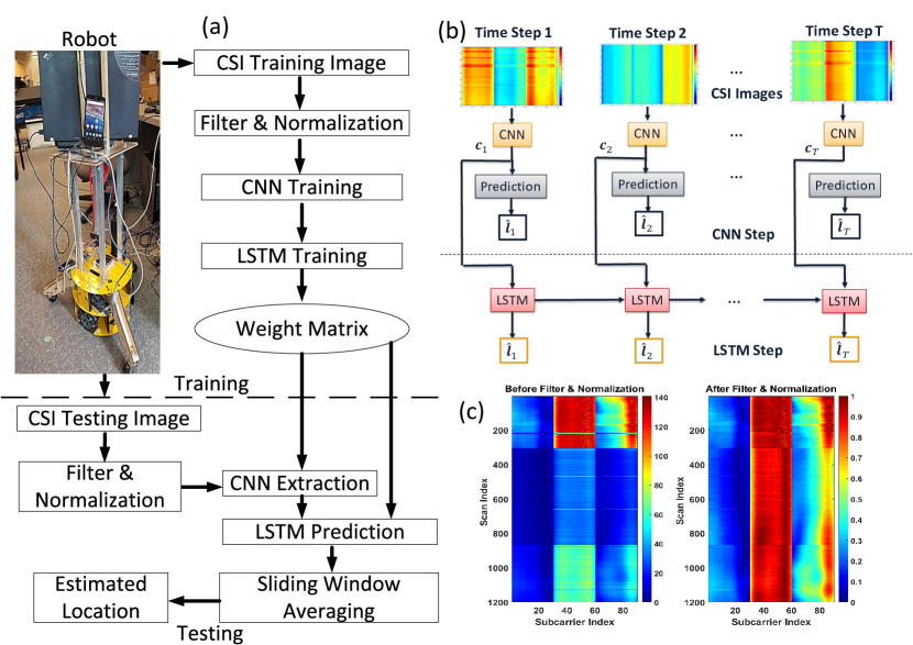
Figure 1: (a) Localization process of the proposed CNN-LSTM system. (b) Proposed CNN-LSTM model. (c) CSI images before and after applying filter and normalization.

The architecture of the proposed CNN-LSTM system is presented in Fig. 1(a). The detailed CNN-LSTM model is shown in Fig. 1(b). The CSI data for both training and testing will be collected with the support of an autonomous robot. Details of the process will be described as follows.

II-C1 CSI Filter And Normalization

By using the modified firmware released for Intel WiFi 5300 NIC card [30] and for Nexus 5 smartphone [18], the mobile devices can get one CSI reading per beacon frame or data frame. Although this CSI provides rich information from multiple subcarriers, it is sensitive to the change of environments such as human blocking and movements, interference from other equipment and devices, receiver antenna orientation, etc., [19]. In order to filter out the outliers caused by the interference and make the measurement more stable, we adopt the median filter [31] for every subcarrier (every column of an CSI image). Then an important normalization process is applied to get cleaner data from the original image. Firstly, the original average amplitude of each image at each location $\bm{l}_{i}$ is calculated as

$${A}_{i}=\frac{\sum_{h=1}^{h=H}\sum_{w=1}^{w=W}{A}^{hw}_{i}}{H{\cdot}W}.$$ (2)

The set of average amplitude of every location in a training database is saved in an array $\{{{A}}_{1},{{A}}_{2},\ldots,{{A}}_{M}\}$. The maximum value in the set is denoted as $A_{max}$ at location $\bm{l}_{max}$. Secondly, every CSI measurement at every location (row of the CSI image) is normalized by the min-max normalization method. In each row $h$ of the image, among $W$ subcarriers, the minimum amplitude is denoted as $Min(A^{hw}_{i})=min([{A}^{h1}_{i},{A}^{h2}_{i},\ldots,A^{hW}_{i}])$ and maximum amplitude is denoted as $Max(A^{hw}_{i})=max([{A}^{h1}_{i},{A}^{h2}_{i},\ldots,A^{hW}_{i}])$. The normalized amplitude of a single pixel at row $h$, column $w$ of the CSI image at location $\bm{l}_{i}$ is given by

$${\hat{A}}^{hw}_{i}=\frac{A^{hw}_{i}-Min(A^{hw}_{i})}{Max(A^{hw}_{i})-Min(A^{hw}_{i})}.$$ (3)

The normalized CSI image at a location will become

$$\centering{\tilde{\hat{A}}}(\bm{l}_{i})=\begin{bmatrix}{\hat{A}}^{11}_{i}&{\hat{A}}^{12}_{i}&\ldots&{\hat{A}}^{1W}_{i}\\ {\hat{A}}^{21}_{i}&{\hat{A}}^{22}_{i}&\ldots&{\hat{A}}^{2W}_{i}\\ \vdots&\vdots&\ddots&\vdots\\ {\hat{A}}^{H1}_{i}&{\hat{A}}^{H2}_{i}&\ldots&{\hat{A}}^{HW}_{i}\\ \end{bmatrix}.\@add@centering$$ (4)

Finally, in order to preserve the original power of the image, the CSI image at each location $\bm{l}_{i}$ is normalized again with the pre-calculated average amplitude set given by

$${\tilde{\hat{A}}}(\bm{l}_{i})={\tilde{\hat{A}}}(\bm{l}_{i})\frac{{A}_{i}}{A_{max}}.$$ (5)

Fig. 1(c) illustrates an example of CSI images collected by Intel WiFi 5300 NIC card before and after applying the filter and normalization process. There are noisy readings (scattered rows), caused by the fluctuation of the CSI amplitude, inside the original CSI image. However, after the median filter and normalization process, the quality of CSI image is improved with more consistent amplitude. The more detailed performance analysis will be discussed more in Subsection IV.

II-C2 Proposed CNN-LSTM Model

The proposed CNN-LSTM architecture is trained by the CSI images from consecutive locations in a trajectory to exploit the time correlation between them. Each location in a trajectory appears in one different time step. The length of a trajectory, or equivalently, the number of time steps, defines the memory length $T$ as illustrated in Fig. 1(b). Because all weights and hidden state values will be saved in every time step in a training trajectory [23], the number of time steps $T$ impacts the performance of LSTM and CNN-LSTM model. Larger $T$ reveals more information from the past but accumulates more errors on prediction [29]. Under the constraints that the distance between consecutive locations is bounded by the maximum distance a user can travel within the sample interval in practical scenarios, the CNN-LSTM training trajectories are randomly generated based on the method proposed in [29].

There are two main layers in our CNN-LSTM model (Fig. 1(b)) including CNN and LSTM layers. While the input of CNN layer is the CSI image from locations in a trajectory, the input of LSTM layer is the output of the previous CNN layer. In other words, CNN will extract the CSI information from spatial domain, whereas LSTM will further exploit that information in the temporal domain. With the information from both domains, the ambiguity of CSI data is significantly mitigated. Subsection IV will show experimental results to demonstrate this mitigation.

The objective of CNN-LSTM training is to minimize the loss function $\mathcal{L}(\bm{\hat{l}},\tilde{\bm{l}})$ which penalizes the Euclidean distance between the output $\bm{\hat{l}}$ and the target $\tilde{\bm{l}}$. Then the backpropagation algorithm uses the chain rule to calculate the derivative of the loss function $\mathcal{L}$ and adjusts the network weights by gradient descent [23]. In [32], Valente et al. show that CNN-LSTM model should be trained separately, instead of using only one common output and one loss function. Therefore, the training of our proposed network is divided into two phases. In phase 1, the CNN layer is trained as a quantification model with CSI images in the database and the loss function mean square error (MSE) described as

$$\mathcal{L}(\bm{l},\tilde{\bm{l}})=||\bm{l}-\tilde{\bm{l}}||_{2}.$$ (6)

The output of the final FC layers in CNN ($\bm{c}_{T}$) is extracted and fed to the input of LSTM (Fig. 1(b)). In phase 2, the trajectory of CNN output spatial features, $\{\bm{c}_{1},\bm{c}_{2},\ldots,\bm{c}_{T}\}$, from $T$ time steps is used for LSTM training. The loss function of this phase is still MSE but for $T$ time steps following MIMO-LSTM model [29] as

$$\mathcal{L}(\bm{\hat{l}},\tilde{\bm{l}})=\frac{\sum_{i=1}^{T}||\bm{\hat{l}}_{i}-\tilde{\bm{l}}_{i}||_{2}}{T}.$$ (7)

III Database And Experiments

Figure 2: (a) Floor map of the CSI test site. The solid blue line is the testing trajectory with blue arrows pointing toward walking direction. (b) Heat map of AP RSSI signal collected from Intel 5300 NIC and Nexus 5 phone. (c) Collected CSI image from Intel 5300 NIC at location (0,0) in 2 different time. (d) Collected CSI image from Nexus 5 phone at location (0,0) in 2 different time. (e) Correlation coefficient of the collected CSI images at location (0,0) along 7 hours.

All experiments have been carried out on the third floor of Engineering Office Wing (EOW), University of Victoria, BC, Canada. The dimension of the area is 21 m by 16 m. It has three long corridors as shown in Fig. 2(a). The CSI fingerprints for both training and testing are collected using an autonomous driving robot. The 3-wheel robot (Fig. 1(a)) has multiple sensors including a wheel odometer, an inertial measurement unit (IMU), a LIDAR, 3 sonar sensors and a color and depth (RGB-D) camera. It can navigate to a target location within an accuracy of $\mathrm{0.21{\pm}0.02~{}m}$.

During the experiments, the robot carried the mobile devices (a Google Nexus 5 smartphone and a Thinkpad T520 laptop equipped with an Intel 5300 NIC) to collect CSI. There is only 1 AP (TPlink AC1750) in the experimental area, operating in channel 36 with a 5 GHz frequency band. Fig. 2(b) illustrates the heat map of the RSSI collected from the Intel 5300 NIC and Nexus 5 smartphone, where the signal strength is represented by color. Clearly, the signals are stronger in the area near the AP. The targeted AP can cover the area including one room (EOW 348) and two corridors with 1185 RPs (pink stars) and 195 testing points (solid blue line). There are 3 receiving antennae on the Intel 5300 NIC, while the smartphone has only one receiving antenna. Therefore, as shown in Fig. 2(b), the RSSI signals from the Intel card are stronger and more consistent than the ones from the smartphone.

In the training phase, the robot stays at every RP to collect data for 2 minutes. The CSI data is repeatedly collected in different days and at different time to build the database. In the testing phase, the robot navigates along a pre-defined route (Fig. 2(a)) at a speed randomly varying within 0.6-4.0 m/s to simulate the indoor walking pattern of a normal person [33, 34]. There are 195 testing points in each testing trajectory. The test experiment is conducted several rounds per day and repeated in 3 different days. Day 1 test mainly targets the quiet time when the area has fewer people (before 9 am and after 5pm). In contrast, during day 2 and 3 we test the localization accuracy at steady time (working hours) and busy time when more people moving around. Note that the validation data is collected at different time from the training data but at the same RP locations, while testing point locations are randomly selected to be different from all RPs in order to approximate our model closer to practical situations. The user location is updated every $\Delta{t}=$1-2 s.

IV Results And Discussions

IV-A CSI Sensitivity

The collected CSI data of each antenna of the Intel 5300 NIC include the IEEE 802.11n channel matrices for 30 subcarrier groups, which is about one group for every two subcarriers at 20 MHz bandwidth [30]. Fig. 2(c) shows some examples of CSI image in RP location (0,0) from this NIC with 1200 scans and 30 subcarriers for each antenna (total 90 subcarriers). Using Nexmon modified firmware [18], we obtain 64 IEEE 802.11ac-subcarriers at bandwidth 20 MHz with 47 of them providing non-zero CSI data from the only one receiving antenna on the Nexus 5 phone. Fig. 2(d) illustrates the CSI images from the phone in the same location (0,0) with 200 scans and 47 non-zero subcarriers.

As mentioned in Subsection II-C1, although CSI provides rich information from multiple subcarriers, it is sensitive to the change of environments especially the interference of human blocking and movements. With the presence of a human, CSI measurement from a subchannel can decrease (or increases) widely [19]. Fig. 2(e) illustrates the fluctuation of CSI data collected from both Intel 5300 NIC and Nexus 5 phone in RP location (0,0) over 7 hours. The experiment was conducted in working hours when many students (up to 10) used WiFi and moved around the area from time to time. CSI images of both devices were sampled every half an hour and were compared with the original CSI images collected at the start time ($t=0$ h) using Pearson coefficient [4]. Fig. 2(e) shows that CSI data of both devices are stable during the long period of time from $t=1.5$ h to $t=4.5$ h, with high correlation coefficients (around $80\%$). It is the period when students in the testing area mostly sat down and studied. However, during the break time, when people started moving around, CSI data changed significantly with the drop to $40\%$ after 5 hours. Fig. 2(c), (d) illustrate the visualization of CSI images at $t=0$ h and $t=5.5$ h. We observe significant change in the pattern of the images (the order of strong and weak subcarriers) in both Intel 5300 NIC and Nexus 5. Therefore, CSI fingerprints in the database might not match with the instant CSI readings in the testing phase because they were collected at different time.

According to our knowledge, this important problem has been neglected in most of the WiFi CSI localization research. This paper is the first one that proposes a feasible solution using an autonomous robot to do the extensive experiments in different time slots. With the sufficient amount of collected training data, the mismatch between database and testing data is significantly reduced.

IV-B CNN Layer Analysis

TABLE II: CNN Layer Parameters

Category	Intel NIC	Nexus 5
Training Data	47,400 CSI images	35,000 CSI images
Validation Data	23,700 CSI images	14,000 CSI images
Conv Layer 1	Input($30\times 30\times 3$)	Input($10\times 47$)
	$5\times 5$ kernels, 10 filters	$5\times 5$ kernels, 10 filters
Conv Layer 2	Input($30\times 30\times 10$)	Input($10\times 47\times 10$)
	$5\times 5$ kernels, 10 filters	$5\times 5$ kernels, 10 filters
Conv Layer 2	Input($30\times 30\times 10$)	Input($10\times 47\times 10$)
	$5\times 5$ kernels, 10 filters	$5\times 5$ kernels, 10 filters
FC Layer 1	9000 neurons	4700 neurons
FC Layer 2	900 neurons	470 neurons
Training Output	Location $\tilde{\bm{l}}$(x,y)	Location $\tilde{\bm{l}}$(x,y)
Loss Function	MSE	MSE

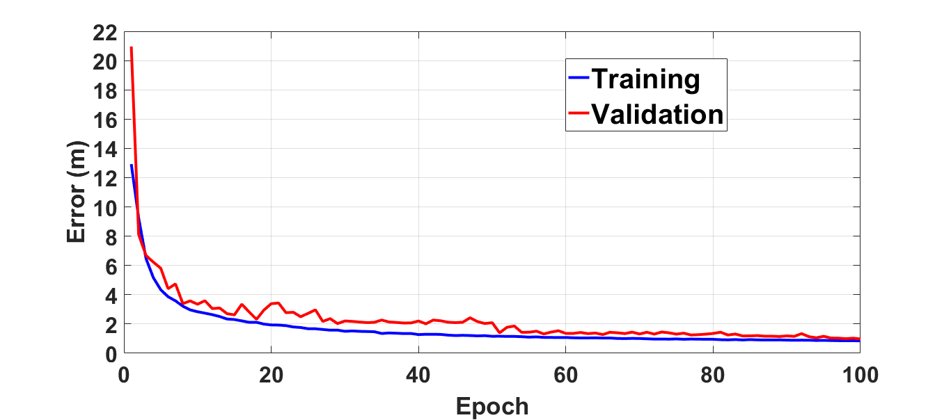
(a)

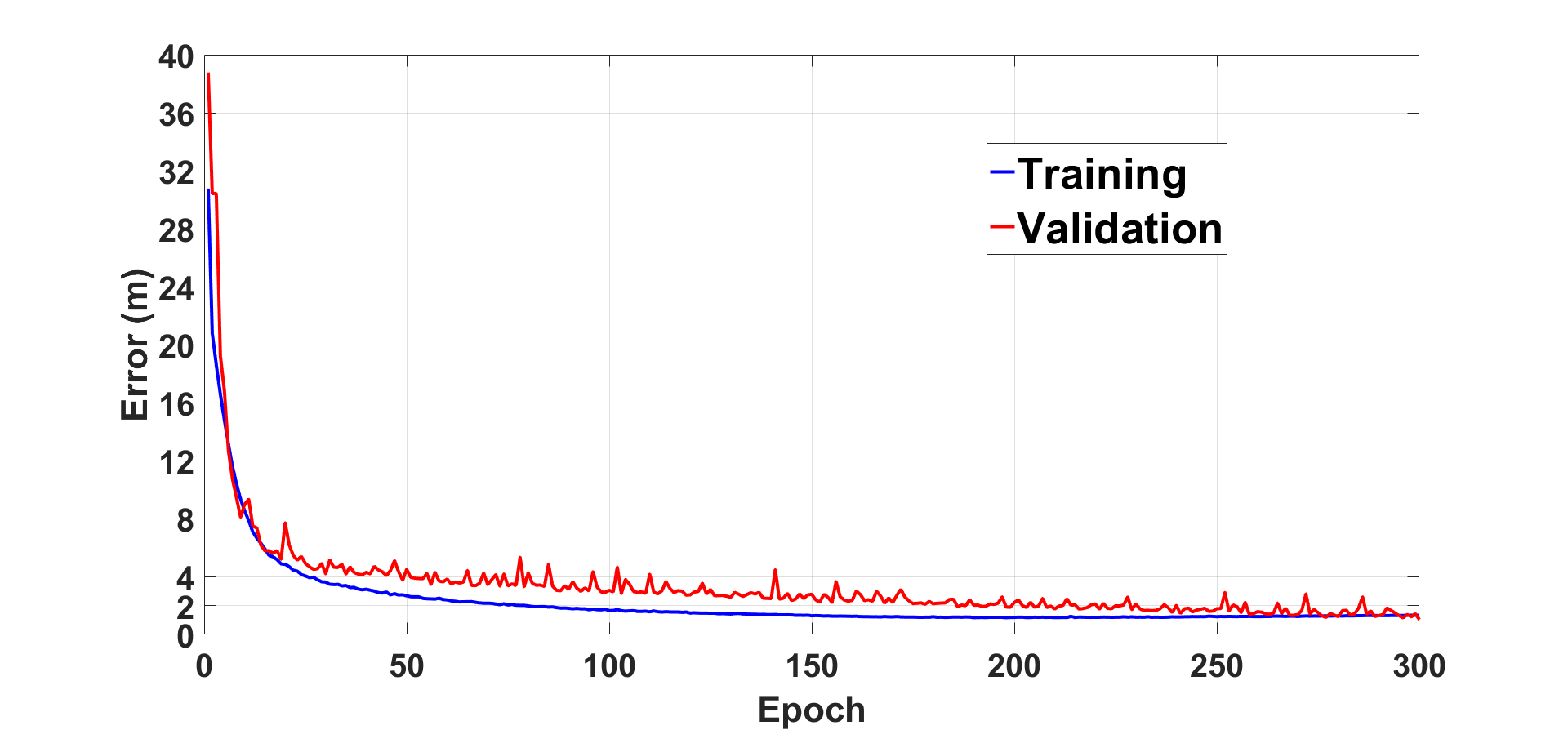
(b)

Figure 3: CNN Layer Learning Curve (a) Intel 5300 NIC. (b) Nexus 5 Phone.

As explained in Section III, the user’s location will be updated every $\Delta{t}=$1-2 s. Therefore, the CSI data collected in the window time $\Delta{t}=$1-2 s is utilized for CNN layer training and validation. During $\Delta{t}$, the NIC receives an average of $30$ packets, and each CSI packet has total 90 subcarriers from 3 receiving antennae. We consider the data from each individual antenna as a channel of the CSI image, which creates the testing CSI image size for the NIC as ($30\times 30\times 3$). On the other hand, the smartphone only receives $10$ scans during $\Delta{t}$ with only one single receiving antenna and $47$ subcarriers. Therefore, the CNN training CSI image size for Nexus 5 is ($10\times 47$).

The CNN model is constructed based on ConFi [3] with 3 convolutional layers (Conv) and 2 FC layers. Table II shows the detailed parameters of the proposed CNN structure for both NIC and smartphone. The differences between them are the inputs of each layer and the number of neurons for the FC layers. There are 9,000 and 900 neurons respectively in the two FC layers for the Intel NIC, while 4,700 and 470 neurons in the case of using the Nexus 5 smartphone.

The number of training data for CNN layers are 47,400 images for the NIC and 35,000 images for the smartphone. There are 23,700 and 14,000 images respectively for the validation. Fig. 3(a) and 3(b) illustrate the learning curves of CNN training for the NIC and smartphone data. Both training processes converge at the localization error around 1.7 m. For Intel 5300 NIC data, the proposed CNN model takes 100 epochs, while there are 300 epochs for the smartphone.

After training, CNN outputs spatial features, $\{\bm{c}_{1},\bm{c}_{2},\ldots,\bm{c}_{T}\}$, of $T$ CSI images from $T$ time steps, which are extracted from the output of the last FC layers (FC layer 2). From every CSI image, there are 900 output spatial features for the NIC and 470 features for the smartphone.

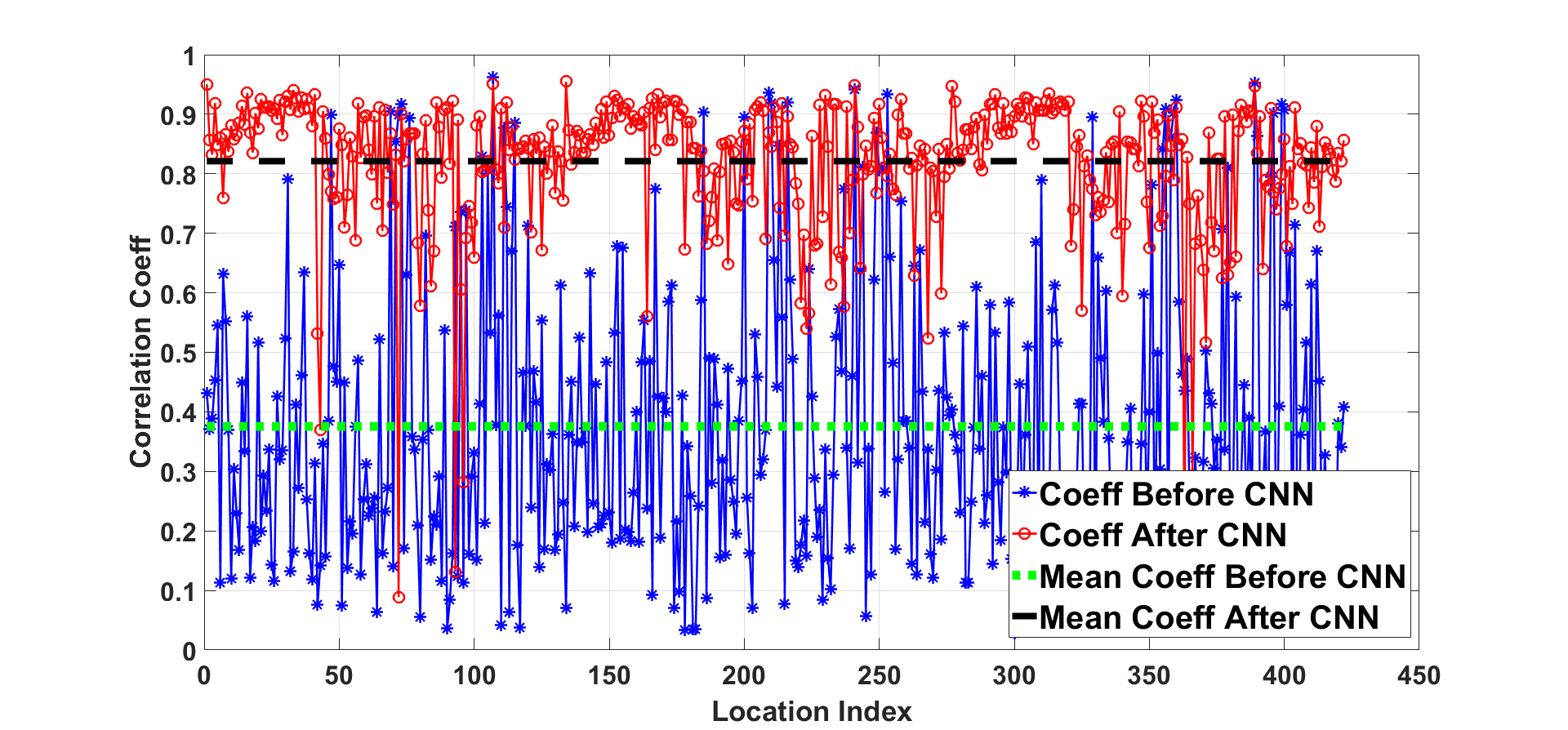
Figure 4: Correlation coefficient of original CSI images before CNN and output spatial features after CNN with Intel 5300 NIC dataset.

Fig. 4 shows the significant increase of the CSI data correlation in 422 random RP locations after CNN layer. Each RP includes 120 CSI images collected at different time. The average correlation coefficient $\rho({\bm{l}_{i}})$ at each location ${\bm{l}_{i}}$ is defined as

$$\rho({\bm{l}_{i}})=\frac{\sum_{j=1}^{N}\sum_{k=1}^{N}\rho_{jk}({\bm{l}_{i}})}{N^{2}}.$$ (8)

where $N=120$ is the number of CSI images at location ${\bm{l}_{i}}$, $\rho_{jk}({\bm{l}_{i}})$ is the Pearson coefficient between the $j^{th}$ image and $k^{th}$ image of that location. Before CNN, due to the CSI sensitivity explained in Subsection IV-A, the correlation between the original CSI images at different time but the same location is as low as around $40\%$. However, after CNN, the important spatial features are extracted from the original images with the irrelevant information being removed. Therefore, the correlation between output spatial features increases to around $80\%$. Similar results are obtained from the smartphone database. The CNN output spatial features, $\{\bm{c}_{1},\bm{c}_{2},\ldots,\bm{c}_{T}\}$, of $T$ will be fed to the next LSTM layer for further processing in time domain.

IV-C LSTM Layer Analysis

TABLE III: Initial setup parameters for RNN system

Category	Intel NIC	Nexus 5
Memory length ($T$)	5	5
Model	MIMO-LSTM	MIMO-LSTM
Loss function	MSE	MSE
Hidden layer	900 neurons	470 neurons
Dropout	0.2	0.2
Optimizer	Adam	Adam
Learning rate	0.001	0.001
Training Data	30,000 trajectories	30,000 trajectories
Validation Data	15,000 trajectories	15,000 trajectories
$\sigma$	2m	2m
$\Delta_{t}$	1s	1s

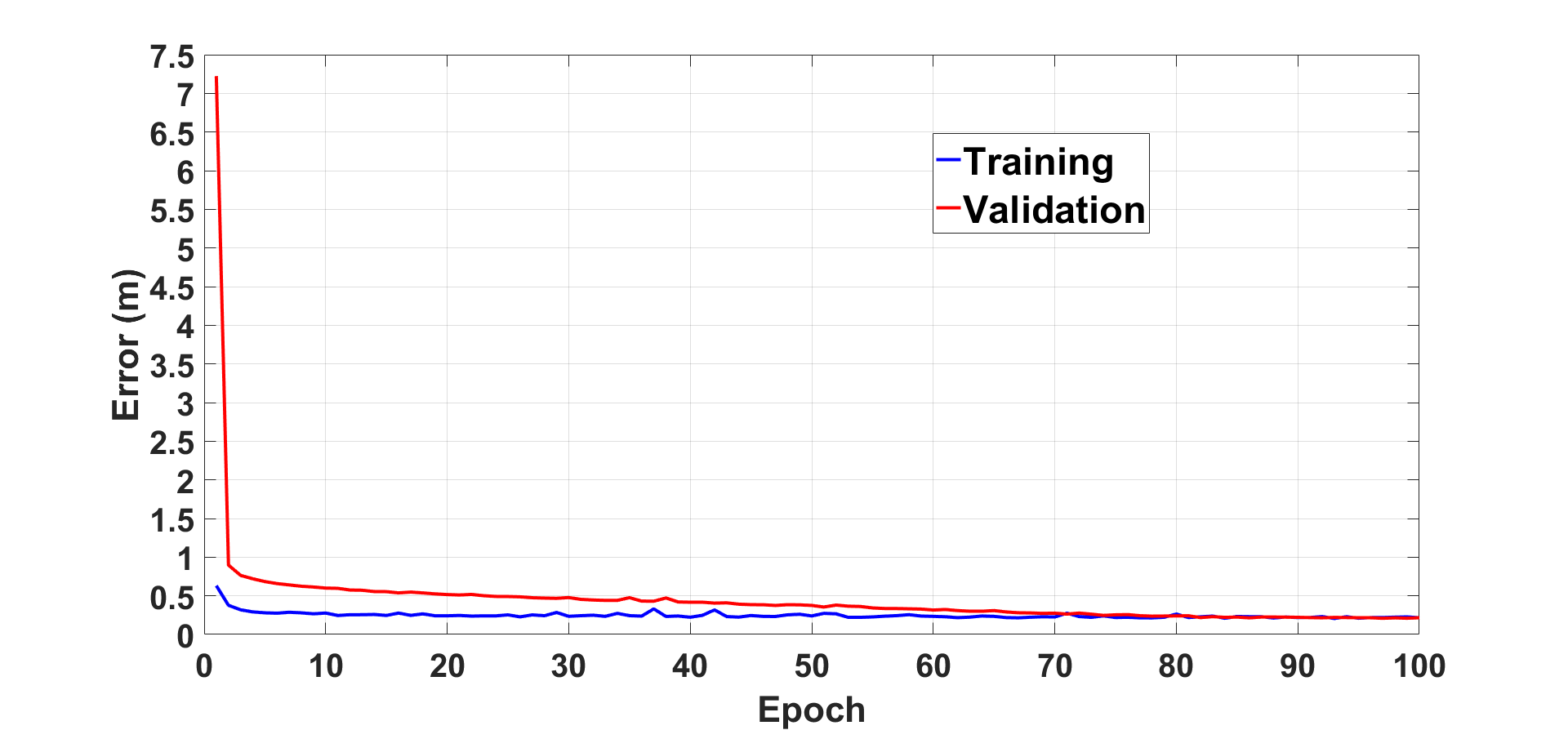
(a)

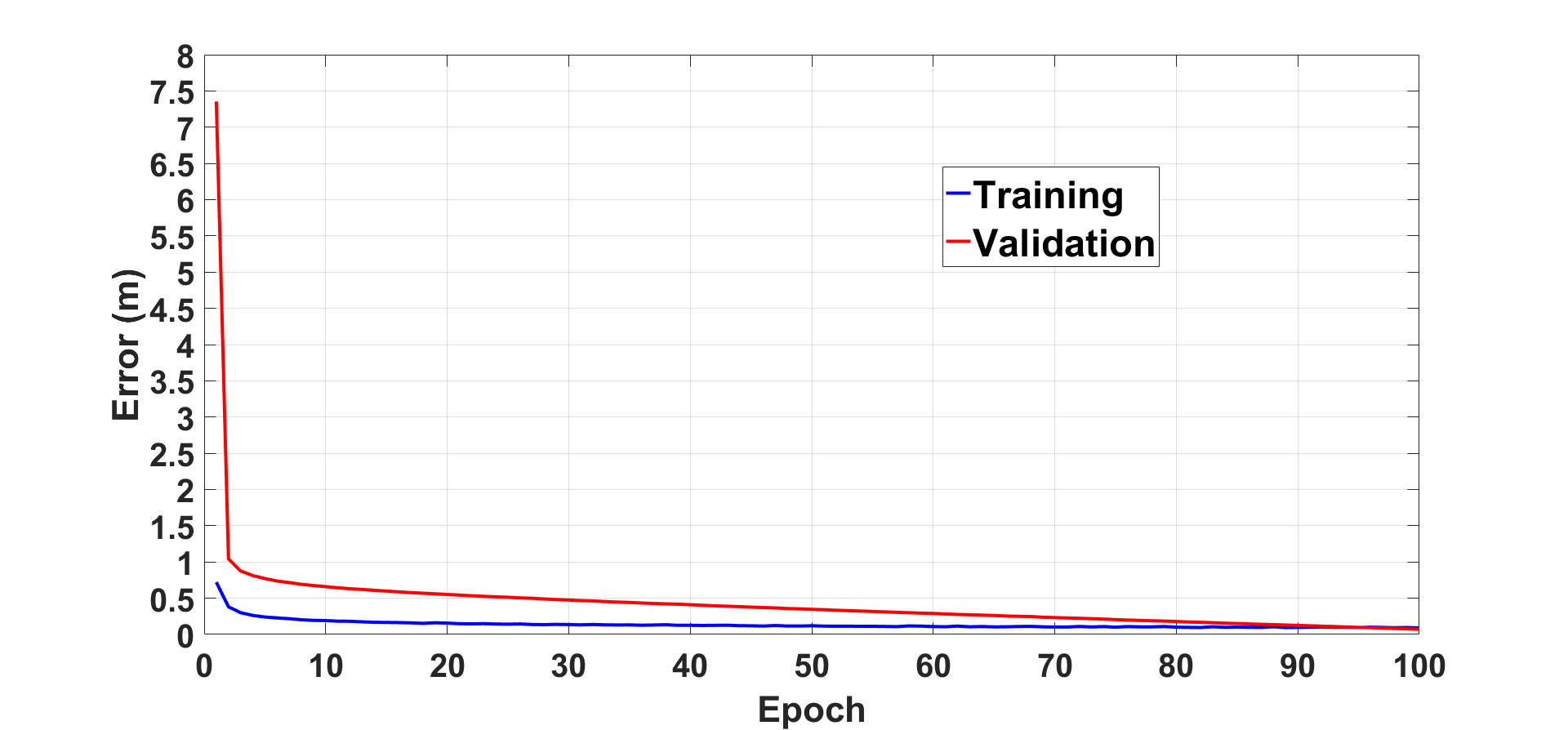
(b)

Figure 5: LSTM Layer Learning Curve (a) Intel 5300 NIC. (b) Nexus 5 Phone.

The detailed parameters for our LSTM network is shown in Table III. The LSTM model follows MIMO-LSTM proposed in [29]. The inputs are multiple generated trajectories containing CNN spatial features from $T$ time steps. Based on the trajectory generation method [29], 30,000 training and 15,000 validation trajectories are generated randomly under the constraints that the distance between consecutive locations is bounded by the maximum distance ($\sigma$) a user can travel within the sample interval $\Delta_{t}=1$ s. In the conducted experiments in [29], the authors show that the memory length $T=5$ and the other longer memory cases including $T=10$ and $T=40$ provide comparable results. Therefore, the memory length here is chosen as $T=5$. The outputs include $T$ time steps locations $\{\bm{\hat{l}}_{1},\bm{\hat{l}}_{2},\ldots,\bm{\hat{l}}_{T}\}$.

Fig. 5(a) and 5(b) show the learning curves of LSTM training for Intel 5300 NIC and Nexus 5 smartphone data. Both training processes converge at a localization error around 0.3 m when the number of epochs reaches 100. It is also the localization accuracy of the proposed method in the case when all of the testing points are the same as reference points. However, in the real scenario, due to the random walk behavior of users, that ideal case rarely happens. Therefore, in order to approximate our method closer to practical situations, all of the reported results below are based on the case when testing points are randomly selected whose positions are considered to be a priori unknown.

IV-D Performance Analysis

TABLE IV: Average Localization Errors of CNN-LSTM

	Intel NIC	Nexus 5
Day 1 - Quiet Time (m)	2.3 $\pm$ 1.7	2.8 $\pm$ 2.1
Day 2 - Steady Time (m)	2.7 $\pm$ 1.7	3.1 $\pm$ 1.7
Day 3 - Busy Time (m)	2.6 $\pm$ 1.6	3.1 $\pm$ 2.2
Average (m)	2.5 $\pm$ 1.6	3.0 $\pm$ 2.0

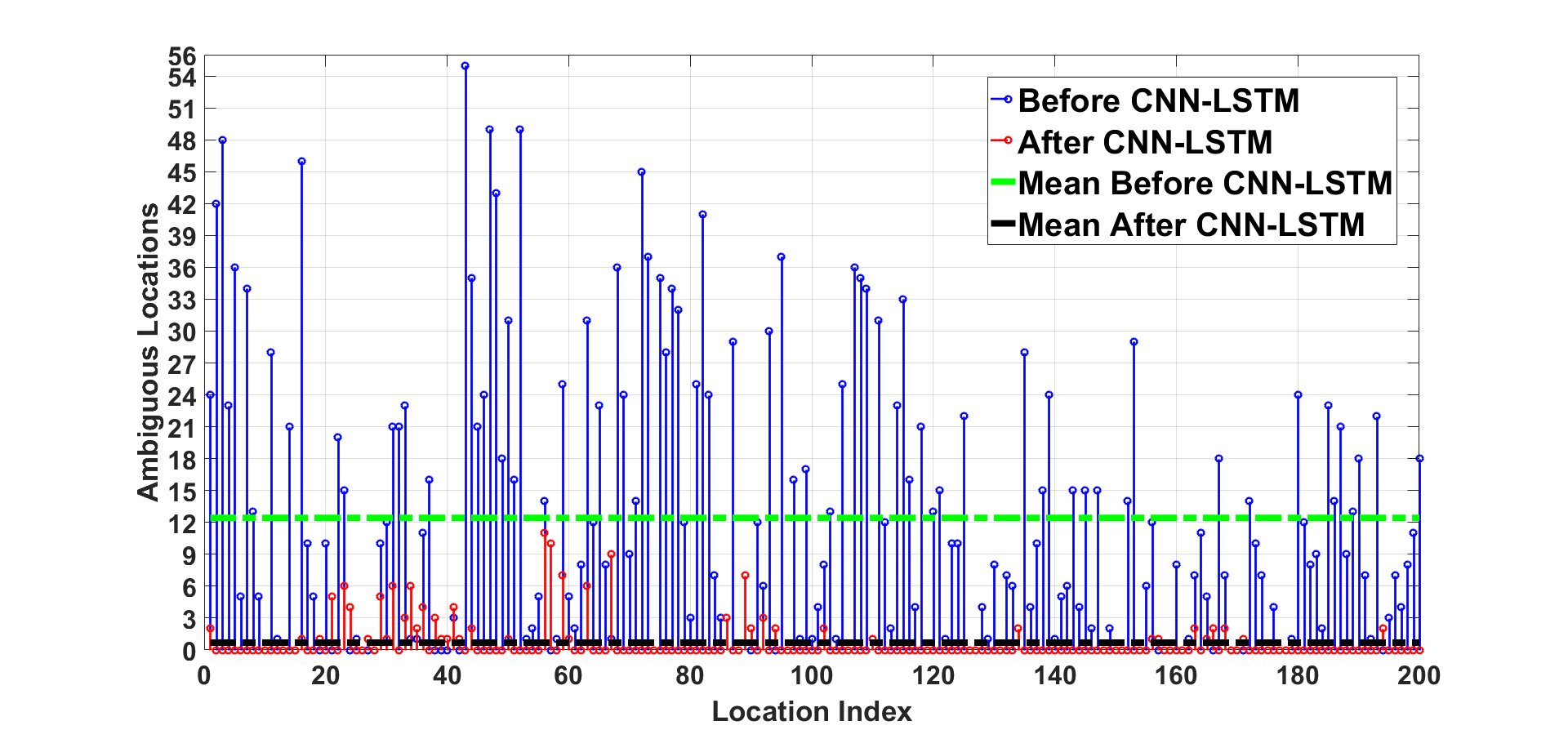
Figure 6: Ambiguous locations in the database before and after CNN-LSTM process with Intel 5300 NIC dataset.

The efficiency of CNN-LSTM layer with both space and time information is evident from the reduction of the ambiguous locations in the database before and after CNN-LSTM training presented in Fig. 6. A location $\bm{l}_{j}$ is defined as an ambiguous point of $\bm{l}_{i}$ if their physical distance is larger than the experimental grid size but their fingerprints have high Pearson correlation coefficient above the correlation threshold. In our experiment, the grid size is 0.5 m. Furthermore, the correlation threshold is chosen based on the average correlation coefficients between $\bm{l}_{i}$ and all of its physical nearest neighbours, which is approximately 0.8 in our database. Then all non-nearest-neighbour locations whose correlation coefficient above this threshold are considered as ambiguous points. The fingerprints before CNN-LSTM process is the original CSI image, while the fingerprints after CNN-LSTM is the spatial output feature in $T=5$ time steps. Pearson correlation coefficient for different fingerprints is explained in details in [29]. Fig. 6 shows the number of ambiguous locations among random 200 RPs of Intel 5300 NIC database. Before CNN-LSTM process, there are many locations sharing similar fingerprints (CSI images) with the average of ambiguous locations around 12. The maximum number of ambiguous locations can be up to more than 55. On the other hand, after extracting spatial and temporal information from the original CSI images, the ambiguity reduces significantly. After CNN-LSTM process, more than $80\%$ of the locations do not have any ambiguous point, which proves that their fingerprints become more distinguishable and unique. There are still few locations having ambiguity but the maximum number of ambiguous locations are only 10 points, which is 5 times smaller than the case before the CNN-LSTM process.

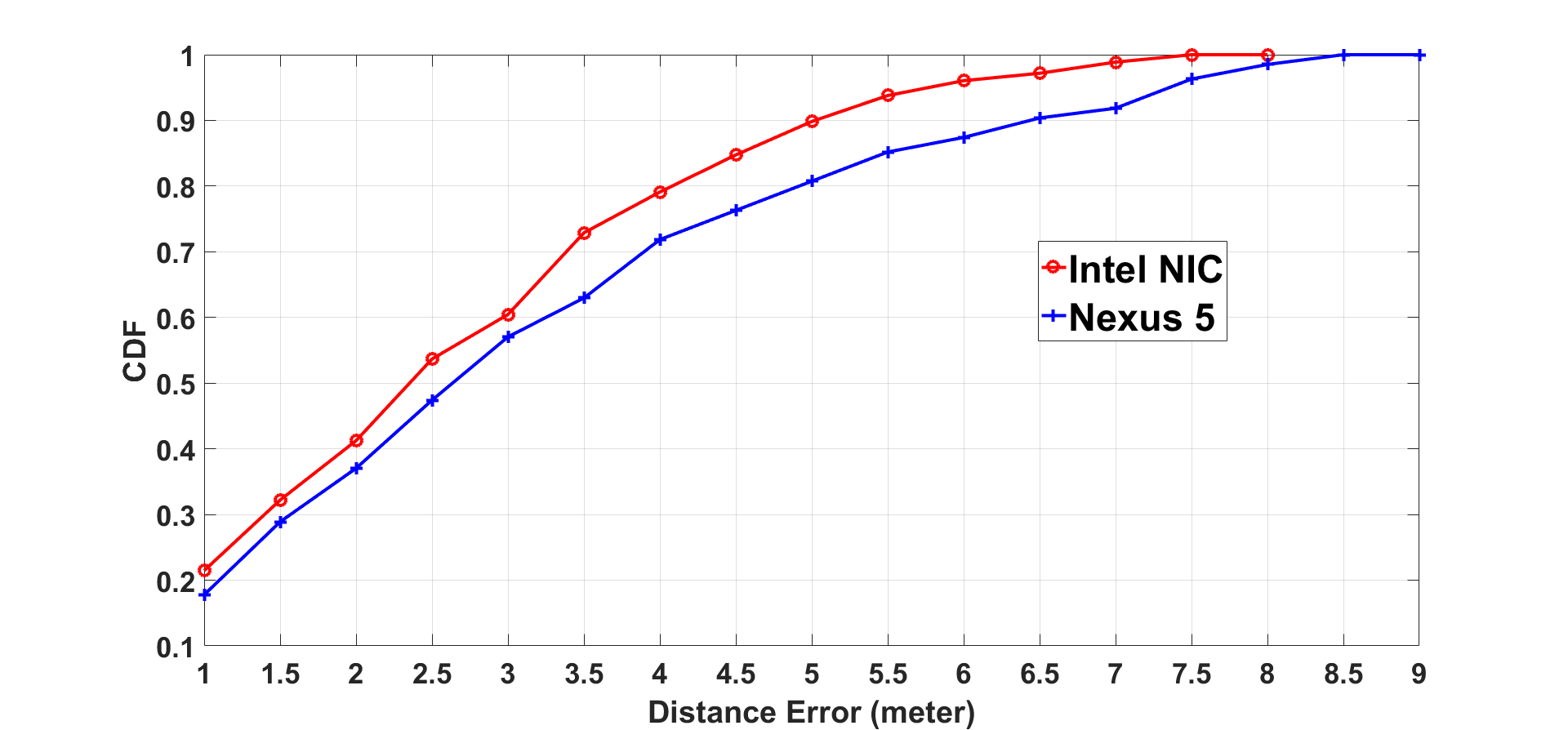
Figure 7: The CDF of the localization error of the proposed CNN-LSTM with Intel NIC and Nexus 5 phone

After the training, CNN-LSTM will be utilized for realtime localization tests. Both the laptop with Intel 5300 NIC and Nexus 5 phone are mounted on the robot which moves at the speed 0.6-4.0 m/s following the testing trajectory in Fig. 2(a). Every $\Delta{t}=$1-2 s, the server will receive CSI packets sending from both Intel NIC and Nexus phone, to predict the current location. Fig. 7 shows the CDF errors of the real testing results. Note again that all of the testing locations are placed randomly and different from all RPs. There are in total 195 collected testing points in each testing trajectory from continuously 3 different days in different time as explained in Section III. The CDF curves in Fig. 7 are the combination errors of all those tests. The Intel 5300 NIC has better performance than the Nexus 5 phone with $80\%$ of the localization error below 4 m compared with 5 m of the smartphone. The maximum localization error of the smartphone can be up to 9 m, while the Intel NIC’s maximum localization error is only around 8 m. Table IV shows the average localization errors of both devices in 3 days of tests. The accuracy of the Intel NIC consistently outperforms the Nexus 5 phone with the average error being around $\mathrm{2.5{\pm}1.6~{}m}$ and $\mathrm{3.0{\pm}2.0~{}m}$ respectively. The main reason that makes the difference in the performance is the number of antennae. The Intel NIC has 3 antennae, while the Nexus 5 smartphone only has a single antenna. Therefore, the CSI information containing in Intel NIC is more than in Nexus 5 phone, which leads to the more accurate localization results.

IV-E Results Comparison

TABLE V: Average Localization Errors - Intel 5300 NIC

	CNN-LSTM	BiLoc [13]	ConFi [3]	FILA [7]
Day 1 - Quiet Time (m)	2.3 $\pm$ 1.7	3.7 $\pm$ 2.6	6.0 $\pm$ 3.8	5.2 $\pm$ 2.7
Day 2 - Steady Time (m)	2.7 $\pm$ 1.7	4.3 $\pm$ 3.0	6.2 $\pm$ 3.5	5.9 $\pm$ 3.2
Day 3 - Busy Time (m)	2.6 $\pm$ 1.6	3.7 $\pm$ 2.9	5.7 $\pm$ 3.2	5.4 $\pm$ 2.8
Average (m)	2.5 $\pm$ 1.6	3.9 $\pm$ 2.8	5.9 $\pm$ 3.5	5.5 $\pm$ 2.9

In order to confirm the effectiveness of our CNN-LSTM model, the proposed method is compared with 3 other popular methods using CSI fingerprint including FILA [7], ConFi [3] and BiLoc [13]. All of those models are implemented under the same test environment as explained in Section III. Both FILA and ConFi leverage CSI amplitude. FILA uses the probabilistic method with Bayes’ rule to estimate the user’s location, while ConFi adopts a CNN model with 5 layers to classify the targeted location. In contrast, BiLoc [13] uses both estimated AoAs and average amplitudes as input data. The mixed network, including deep autoencoder, restricted Boltzmann machine along with radial basis function, is used to get the bi-modal fingerprints. Finally, the user’s location is determined by the probabilistic model with Bayes’ rule. In their research, the CSI data are obtained from Intel 5300 NIC. Therefore, as a fair comparison, all of the latter figures and tables are presented with Intel 5300 NIC database results.

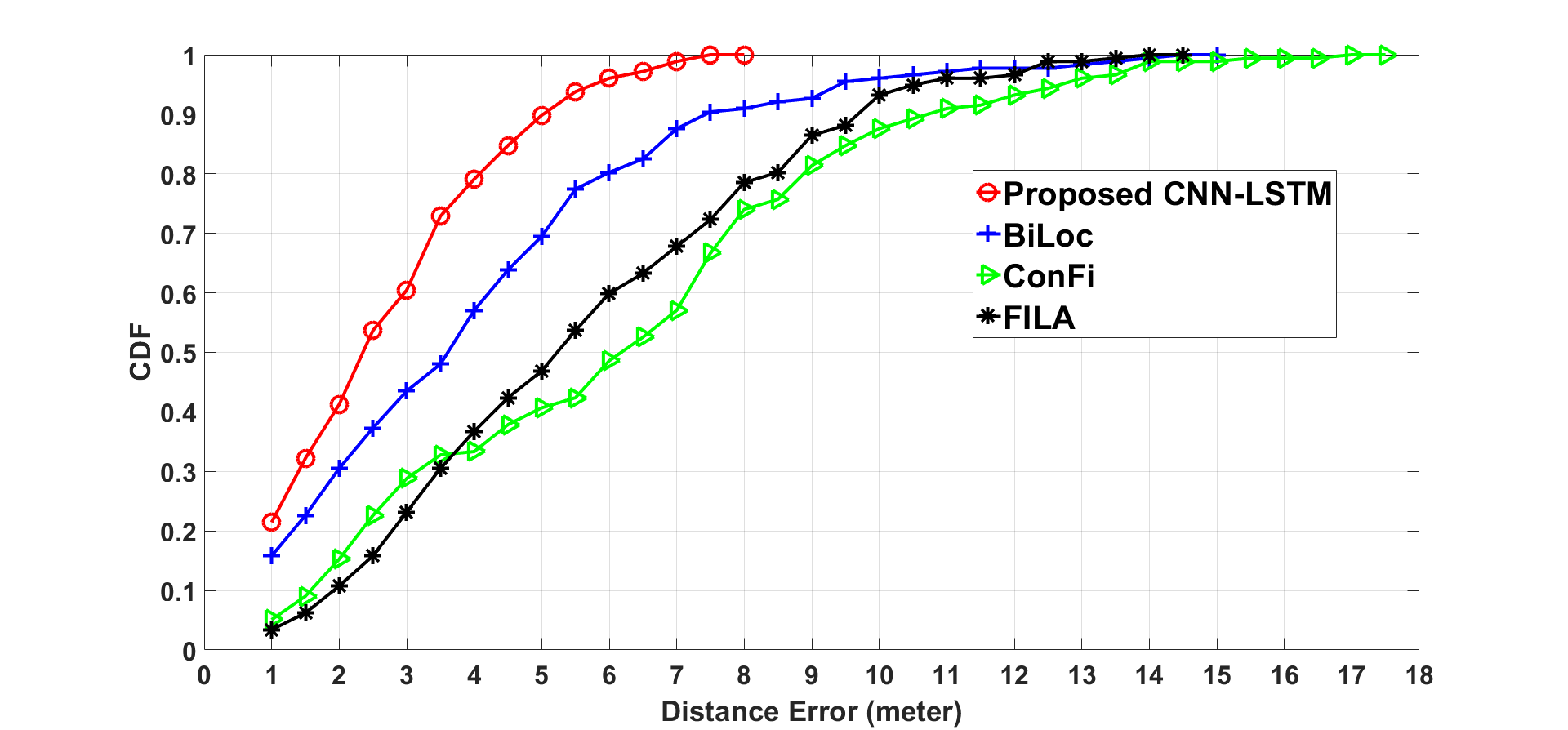
Figure 8: The CDF of the localization error of the proposed CNN-LSTM and the other methods in literature.

Table V shows the average error comparison between the proposed method and the three others. All experiments are conducted in 3 days with 195 testing locations, and the proposed model consistently has dominant performance compared with all other 3 approaches. CNN-LSTM has an average error around $\mathrm{2.5{\pm}1.6~{}m}$, nearly 2.5 times lower than ConFi and FILA whose errors are $\mathrm{5.9{\pm}3.5~{}m}$ and $\mathrm{5.5{\pm}2.9~{}m}$, respectively. Furthermore, the accuracy of our proposed CNN-LSTM is also $50\%$ better than BiLoc which has an average error of $\mathrm{3.9{\pm}2.8~{}m}$. Besides, Fig. 8 illustrates the CDF error comparison of all four methods. CNN-LSTM with the information of both space and time reduces the maximum error significantly, from more than 17 m of ConFi and 15 m of BiLoc to only 8 m of the proposed approach. Further, $80\%$ of the localization error of CNN-LSTM is below 4 m, which is much lower than that of BiLoc with 6 m and around 8 m of both ConFi and FILA.

V Conclusions

In conclusion, we have proposed a combined CNN-LSTM quantification model for accurate single router WiFi fingerprinting indoor localization. Our CNN-LSTM network extracts both spatial and temporal information of received CSI signals to determine a user’s moving path. The extensive on-site experiments, with several mobile devices including mobile phone (Nexus 5) and laptop (Intel 5300 NIC) in hundreds of testing locations, have been presented. The experimental results have consistently demonstrated that our CNN-LSTM structure achieves an average localization error of 2.5 m with $\mathrm{80\%}$ of the errors under 4 m, which outperforms the other algorithms by at least $\mathrm{50\%}$ under the same test environment. In the future research, we will utilize the proposed CNN-LSTM model in more test scenarios with different kinds of fingerprints including both RSSI and CSI to improve the performance.

References

- [1] Y. Xu, Autonomous Indoor Localization Using Unsupervised Wi-Fi Fingerprinting. Kassel University Press, 2016.
- [2] C. Liu, D. Fang, Z. Yang, H. Jiang, X. Chen, W. Wang, T. Xing, and L. Cai, “RSS distribution-based passive localization and its application in sensor networks,” IEEE Transactions on Wireless Communications, vol. 15, pp. 2883 – 2895, Apr. 2016.
- [3] H. Chen, Y. Zhang, W. Li, X. Tao, and P. Zhang, “ConFi: Convolutional neural networks based indoor Wi-Fi localization using channel state information,” IEEE Access, vol. 5, pp. 18 066 – 18 074, Sep. 2017.
- [4] M. T. Hoang, Y. Zhu, B. Yuen, T. Reese, X. Dong, T. Lu, R. Westendorp, and M. Xie, “A soft range limited K-nearest neighbours algorithm for indoor localization enhancement,” IEEE Sensors Journal, vol. 18, pp. 10 208–10 216, Dec. 2018.
- [5] S.-H. Fang and T.-N. Lin, “Indoor location system based on discriminant-adaptive neural network in IEEE 802.11 environments,” IEEE Transactions on Neural Networks, pp. 1973–1978, Nov 2008.
- [6] S. Han, Y. Li, W. Meng, C. Li, T. Liu, and Y. Zhang, “Indoor localization with a single Wi-Fi Access Point based on OFDM-MIMO,” IEEE Systems Journal, vol. 13, pp. 964 – 972, Mar. 2019.
- [7] K. Wu, J. Xiao, Y. Yi, D. Chen, X. Luo, and L. M. Ni, “CSI - based indoor localization,” IEEE Transactions on Parallel and Distributed Systems, vol. 24, pp. 1300 – 1309, Jul. 2013.
- [8] M. Youssef and A. Agrawala, “The Horus WLAN location determination system,” Proc. 3rd international conference on Mobile systems, applications, and services, pp. 205–218, 2005.
- [9] X. Wang, L. Gao, S. Mao, and S. Pandey, “CSI-based fingerprinting for indoor localization: A deep learning approach,” IEEE Transactions on Vehicular Technology, vol. 66, pp. 763 – 776, Jan. 2017.
- [10] M. T. Hoang, B. Yuen, X. Dong, T. Lu, R. Westendorp, and K. Reddy, “Semi-sequential probabilistic model for indoor localization enhancement,” IEEE Sensors Journal, Early Access, pp. 1–1, Mar 2020.
- [11] X. Wang, L. Gao, and S. Mao, “CSI phase fingerprinting for indoor localization with a deep learning approach,” IEEE Internet of Things Journal, vol. 3, pp. 1113 – 1123, Dec. 2016.
- [12] X. Wang, X. Wang, and S. Mao, “Deep convolutional neural networks for indoor localization with CSI images,” IEEE Transactions on Network Science and Engineering, vol. 7, no. 1, pp. 316–327, Jan 2020.
- [13] X. Wang, L. Gao, and S. Mao, “BiLoc: Bi-modal deep learning for indoor localization with commodity 5GHz WiFi,” IEEE Access, vol. 5, pp. 4209–4220, 2017.
- [14] D. Vasisht, S. Kumar, and D. Katabi, “Sub-nanosecond Time of Flight on commercial Wi-Fi cards,” Proceedings of the 2015 ACM Conference on Special Interest Group on Data Communication, pp. 121–122, Aug. 2015.
- [15] F. Ricciato, S. Sciancalepore, F. Gringoli, N. Facchi, and G. Boggia, “Position and velocity estimation of a non-cooperative source from asynchronous packet arrival time measurements,” IEEE Transactions on Mobile Computing, vol. 17, pp. 2166 – 2179, Jan. 2018.
- [16] X. Li and K. Pahlavan, “Super-resolution TOA estimation with diversity for indoor geolocation,” IEEE Transactions on Wireless Communications, vol. 3, pp. 224 – 234, Jan. 2004.
- [17] X. Wang, L. Gao, and S. Mao, “BiLoc: Bi-modal deep learning for indoor localization with commodity 5 GHz WiFi,” IEEE Access, vol. 5, pp. 4209 – 4220, Mar. 2017.
- [18] M. Schulz, D. Wegemer, and M. Hollick, “The Nexmon firmware analysis and modification framework: Empowering researchers to enhance Wi-Fi devices,” Computer Communications ScienceDirect, vol. 129, pp. 269 – 285, Sep. 2018.
- [19] S. Shi, S. Sigg, L. Chen, and Y. Ji, “Accurate location tracking from CSI-based passive device-free probabilistic fingerprinting,” IEEE Transactions on Vehicular Technology, vol. 67, pp. 5217 – 5230, Jun. 2018.
- [20] L. Yan, L. Bottou, Y. Bengio, and et al, “Gradient-based learning applied to document recognition,” Proceedings of the IEEE, vol. 86, pp. 2278 – 2324, Nov. 1998.
- [21] P. Y. Simard, D. Steinkraus, and J. C. Platt, “Best practices for convolutional neural networks applied to visual document analysis,” Proc. 7th Int. Conf. Document Anal. Recognit., pp. 958 – 963, 2003.
- [22] H. J. Jang, J. M. Shin, and L. Choi, “Geomagnetic field based indoor localization using recurrent neural networks,” GLOBECOM 2017, pp. 1–6, Dec. 2017.
- [23] Z. C. Lipton, J. Berkowitz, and C. Elkan, “A critical review of recurrent neural networks for sequence learning,” arXiv:1506.00019, Oct. 2015.
- [24] J. Chung, C. Gulcehre, K. Cho, and Y. Bengio, “Empirical evaluation of gated recurrent neural networks on sequence modeling,” arXiv:1412.3555v1, Dec. 2014.
- [25] S. Hochreiter and J. Schmidhuber, “Long short-term memory,” Neural Comput., vol. 9, pp. 1735–1780, Nov. 1997.
- [26] K. Cho, B. van Merrienboer, D. Bahdanau, and Y. Bengio, “On the properties of neural machine translation: Encoder–decoder approaches,” Proceedings of SSST-8, Eighth Workshop on Syntax, Semantics and Structure in Statistical Translation, p. 103–111, Oct. 2014.
- [27] M. Schuster and K. Paliwal, “Bidirectional recurrent neural networks,” IEEE Transactions on Signal Processing, vol. 45, pp. 2673 – 2681, Nov. 1997.
- [28] W. Zhao, S. Han, R. Q. Hu, W. Meng, and Z. Jia, “Crowdsourcing and multi-source fusion based fingerprint sensing in smartphone localization,” IEEE Sensors Journal, vol. 18, pp. 3236 – 3247, Feb. 2018.
- [29] M. T. Hoang, B. Yuen, X. Dong, T. Lu, R. Westendorp, and K. Reddy, “Recurrent neural networks for accurate RSSI indoor localization,” IEEE Internet of Things Journal, vol. 6, no. 6, pp. 10 639–10 651, Dec 2019.
- [30] D. Halperin, W. Hu, A. Sheth, and D. Wetherall, “Tool release: Gathering 802.11n traces with channel state information,” ACM SIGCOMM Comput. Commun. Rev., vol. 41, no. 1, p. 53, Jan. 2011.
- [31] J. D. Broesch, Applications of DSP. ScienceDirect, 2008.
- [32] M. Valente, C. Joly, and A. de La Fortelle, “An LSTM network for real-time odometry estimation,” 2019 IEEE Intelligent Vehicles Symposium (IV), pp. 1434–1440, June 2019.
- [33] R. C. Browning, E. A. Baker, J. A. Herron, and R. Kram, “Effects of obesity and sex on the energetic cost and preferred speed of walking,” Journal of Applied Physiology, vol. 100, pp. 390–398, Feb. 2006.
- [34] B. J. Mohler, W. B. Thompson, S. H. Creem-Regehr, H. L. PickJr, and W. H. Warren, “Visual flow influences gait transition speed and preferred walking speed,” Experimental Brain Research, vol. 181, pp. 221–228, Aug. 2007.