Classification of particle trajectories in living cells: machine learning versus statistical testing hypothesis for fractional anomalous diffusion

Abstract

Single-particle tracking (SPT) has become a popular tool to study the intracellular transport of molecules in living cells. Inferring the character of their dynamics is important, because it determines the organization and functions of the cells. For this reason, one of the first steps in the analysis of SPT data is the identification of the diffusion type of the observed particles. The most popular method to identify the class of a trajectory is based on the mean square displacement (MSD). However, due to its known limitations, several other approaches have been already proposed. With the recent advances in algorithms and the developments of modern hardware, the classification attempts rooted in machine learning (ML) are of particular interest. In this work, we adopt two ML ensemble algorithms, i.e. random forest and gradient boosting, to the problem of trajectory classification. We present a new set of features used to transform the raw trajectories data into input vectors required by the classifiers. The resulting models are then applied to real data for G protein-coupled receptors and G proteins. The classification results are compared to recent statistical methods going beyond MSD.

I Introduction

Single-particle tracking (SPT) has become an important tool in the biophysical community in recent years. It was first carried out on proteins diffusing in the cell membrane Barak and Webb (1982); Kusumi et al. (1993). Since then it was successfully used to study different transport processes in intracellular environment, providing valuable information about mechano-structural characteristics of living cells. For instance, it helped already to unveil the details of the movement of molecular motors inside cells Yildiz et al. (2003); Kural et al. (2005) or of target search mechanisms of nuclear proteins Izeddin et al. (2014).

Living cells belong to the class of active systems Gal et al. (2013), in which the particles undergo simultaneous active and thermally driven transport. It has been shown already that the dynamics of proteins in cells determines their organization and functions Bressloff (2014). This is the reason why it is crucial to identify the type of motion of the observed particles in order to deduct their driving forces Saxton (1994); Saxton and Jacobson (1997); Feder et al. (1996); Metzler and Klafter (2000).

Over the last decades, a number of stochastic models has been already proposed to describe the intracellular transport of molecules Michalet (2010); Metzler and Klafter (2000). Within those models, the dynamics of molecules usually alternates between distinct types of diffusion, each of which may be associated with a different physical scenario. The Brownian motion Alves et al. (2016) models a particle that diffuses freely, i.e. it does not meet any obstacles in its path nor it interacts with other molecules in its surrounding. The subdiffusion is appropriate to represent trapped particles Hoze et al. (2012); Metzler and Klafter (2000), particles which encounter fixed or moving obstacles Saxton (1994); Berry and Chaté (2014) or particles slowed down due to the viscoelastic properties of the cytoplasm Weiss et al. (2004). Finally, the superdiffusion models the motion driven by molecular motors: the particles move faster than in a free diffusion case and in a specific direction Arcizet et al. (2008). The sub- and superdiffusion together are often referred to as the anomalous diffusion.

The standard method of classification of individual trajectories into those three types of diffusion is based on the mean square displacement (MSD) Michalet (2010). Within this approach one fits the theoretical MSD curves for various models to the data and then selects the best fit with statistical analysis Monnier et al. (2012). A linear MSD curve indicates the free diffusion, a sublinear (superlinear) one - the subdiffusion (the superdiffusion). However, there are some issues related with this method. In many cases, the experimental trajectories are too short to extract a meaningful information from MSD. Moreover, the finite precision adds a term to the MSD, which is known to limit the interpretation of the data Michalet (2010); Saxton and Jacobson (1997); Kepten et al. (2015); Briane et al. (2018). As a result, several methods improving or going beyond the MSD have been introduced to overcome these problems. For instance, Michalet Michalet (2010) used an iterative method called the optimal least-squares fit to determine the optimal number of points to obtain the best fit to MSD in the presence of localization errors. Weiss Weiss (2019) used a resampling approach that eliminates localization errors in the time-averaged MSD of subdiffusive fractional Brownian motion processes. The trajectory spread in space calculated through the radius of gyration Saxton (1993), the Van Hove displacements distributions and deviations from Gaussian statistics Valentine et al. (2001), self-similarity of trajectory using different powers of the displacement Gal and Weihs (2010), velocity autocorrelation function Grebenkov et al. (2013); Fuliński (2017) or the time-dependent directional persistence of trajectories Raupach et al. (2007) methods can be combined with the output of MSD to improve the classification results. The distribution of directional changes Burov et al. (2013), the mean maximum excursion method Tejedor et al. (2010) and the fractionally integrated moving average (FIMA) framework Burnecki et al. (2015) may efficiently replace the MSD estimator for classification purposes. Hidden Markov Models (HMM) has been proposed to check the heterogeneity within single trajectories Das et al. (2009); Slator et al. (2015). They have proven to be quite useful in the detection of confinement Slator and Burroughs (2018). Last but not least, classification based on hypothesis testing, both relying on MSD and going beyond this statistics, has been shown to be quite successful as well Briane et al. (2018); Weron et al. (2019).

An alternative, very promising approach to SPT data analysis is rooted in computer science. Namely, classification of trajectories may be seen as a subject of machine learning (ML) Raschka (2015). In the ML context, classification relies on available data, because its goal is to identify to which category a new observation belongs on the basis of a training data set containing observations with a known category membership.

There is already a number of attempts to analyze particle trajectories with machine learning methods. Among them, Bayesian approach Monnier et al. (2012); Thapa et al. (2018); Cherstvy et al. (2019), random forests Wagner et al. (2017); Kowalek et al. (2019); Muñoz-Gil et al. (2020), neural networks Dosset et al. (2016) and deep neural networks Kowalek et al. (2019); Granik et al. (2019); Bo et al. (2019); Han et al. (2020) have gained a lot of attention and popularity. While some of the works have focused just on the identification of the diffusion modes Dosset et al. (2016); Wagner et al. (2017); Kowalek et al. (2019), the others went beyond just the classification of diffusion and tried to extract quantitative information about the trajectories (e.g. the anomalous exponent Muñoz-Gil et al. (2020); Granik et al. (2019)).

Recently, we presented a comparison of performance of two different classes of methods: traditional feature-based algorithms (random forest and gradient boosting) and a modern deep learning approach based on convolutional neural networks Kowalek et al. (2019). The latter constitutes nowadays the state-of-the-art technology for automatic data classification and is much simpler to use from the perspective of the end-user, because it operates on raw data and does not require any preprocessing effort from human experts Hatami et al. (2018). In contrast, the traditional methods require a representation of trajectories by a set of human-engineered features or attributes Mitchel (1997). In most of the applications the deep learning approach outperforms the traditional methods. However, in some situations it is still worth to use them, because they usually work better on small data sets, are computationally cheaper and easier to interpret. From our results it follows that both approaches achieve excellent (and very similar) accuracies on synthetic data. But they turned out to be really bad in terms of transfer learning. This concept refers to a situation, in which a classifier is trained in one setting and then applied to a different one. The classifiers from Ref. Kowalek et al. (2019) were not able to successfully classify trajectories generated with methods different from the ones used for the training set.

In this paper, we are going to present an improved version of the traditional classifiers presented in Ref. Kowalek et al. (2019). We will propose a new set of training data as well as a new collection of features describing a trajectory. Both are inspired by a recent statistical analysis of anomalous diffusion Weron et al. (2019). To illustrate the transfer learning abilities of the new classifiers, we will apply them to the data from a single-particle tracking experiment on G protein-coupled receptors and G proteins Sungkaworn et al. (2017). Results of classification from Ref. Weron et al. (2019) will be used as a benchmark.

The paper is organized as follows. In Sec. II, we briefly introduce the different modes of diffusion and methods of their analysis. Sec. III contains a short description of the machine learning methods used in this work. Stochastic models of diffusion for generation of synthetic data are presented in Sec. IV. The data itself is characterized in Sec. V. The set of features used as input to the classifiers is introduced in Sec. VI. Our results are presented in Sec. VII, followed by some concluding remarks.

II Diffusion modes and their analysis

As already mentioned in the introduction, identification of the diffusion modes of particles within living cells is important, because they reflect the interactions of those particles with their surrounding. For instance, if a particle is driven by a free diffusion (Brownian motion) Alves et al. (2016), we expect that it does not meet any obstacles in its path and does not undergo any relevant interactions with other particles. Deviations from Brownian motion are called anomalous diffusion and can be divided into two distinct classes. Subdiffusion is slower than the normal one. It usually occurs in crowded or constrained domains and can be brought together with different physical mechanisms including immobile obstacles, cytoplasm viscosity, crowding, trapping and heterogeneities Höfling and Franosch (2013); Szymanski and Weiss (2009); Jeon and Metzler (2010). Superdiffusion represents active transport along the cytoskeleton, assisted by molecular motors Arcizet et al. (2008). Particles undergoing that type of motion move faster than those freely diffusing and usually do not come back to previous positions.

Although different scenarios for both classes of anomalous diffusion are possible Metzler and Klafter (2000); Weigel et al. (2011, 2012); Hellmann et al. (2011); Szymanski and Weiss (2009); Sadegh et al. (2017), for the purpose of this work we will limit ourselves to those three basic types mentioned above: free, sub- and superdiffusion.

The most popular method of deducing a particles’ type of motion from their trajectories is based on the analysis of the mean square displacement (MSD) Qian et al. (1991),

$$MSD(t)=\mathrm{E}\left(\|X_{t+t_{0}}-X_{t_{0}}\|^{2}\right),$$ (1)

where $(X_{t})_{t>0}$ is a particle trajectory, $\|\cdot\|$ is the Euclidean norm and $\mathrm{E}$ is the expectation of the probability space. Since in many experiments only a limited number of trajectories is observed, the time averaged MSD (TAMSD) calculated from a single trajectory is usually used as the estimator of MSD,

$$\widehat{MSD}(n\Delta t)=\frac{1}{N-n+1}\sum_{i=0}^{N-n}\|X_{t_{i+n}}-X_{t_{i}}\|^{2}.$$ (2)

The trajectory is assumed to be given in form of $N$ consecutive two dimensional positions $X_{i}=(x_{i},y_{i})$ ($i=0,\dots,N$) recorded with a constant time interval $\Delta t$ and $n$ is the time lag between the initial and the final positions of the particle. If the underlying process is ergodic and has stationary increments, TAMSD converges to the theoretical MSD Weigel et al. (2011).

TAMSD as a function of the time lag for the normal diffusion converges asymptotically to a linear function Saxton and Jacobson (1997), i.e. for large $N$:

$$\widehat{MSD}(n\Delta t)\sim 4D(n\Delta t),$$ (3)

with $D$ being the diffusion coefficient. For subdiffusion, being slower than diffusion, the behaviour of TAMSD is sublinear, while for superdiffusion, being faster than diffusion, the behaviour is superlinear. Thus, for pure trajectories with no localization errors one could easily determine their diffusion type by fitting a function $\alpha\log(n\Delta t)+\beta$ to the estimated $\log[\widehat{MSD}(n\Delta t)]$ curve. If $\alpha<1$ then the trajectory can be identified as subdiffusive, while if $\alpha>1$, as superdiffusive. Although theoretically this approach allows for the uncomplicated distinction of the diffusion types, there are several issues related with it as a method for classification. First, real trajectories are usually noisy, which makes the fitting of a mathematical model a challenging task, even in the simplest case of the normal diffusion Michalet (2010); Weiss (2019). Secondly, according to Eq. (2), only the values of $\widehat{MSD}$ corresponding to small time lags are well averaged. The larger the lag, the smaller is the number of displacements contributing to the averages, resulting in fluctuations increasing with the lag. Selecting a suitable lag is by the way a well known problem in biophysics Briane et al. (2018); Vega et al. (2018); Lanoiselée et al. (2018). Since many real trajectories are short, we are forced to concentrated on short times (small lags). This induces another problem in a classification method based only on MSD curves, as in this case the different power laws look alike even in the absence of noise.

III Machine learning approach

Several different procedures have been already proposed to circumvent the limitations of the MSD Michalet (2010); Saxton (1993); Valentine et al. (2001); Gal and Weihs (2010); Raupach et al. (2007); Burov et al. (2013); Tejedor et al. (2010); Das et al. (2009); Slator et al. (2015); Slator and Burroughs (2018); Briane et al. (2018); Weron et al. (2019), including the use of machine learning methods Monnier et al. (2012); Thapa et al. (2018); Cherstvy et al. (2019); Wagner et al. (2017); Kowalek et al. (2019); Muñoz-Gil et al. (2020); Granik et al. (2019); Bo et al. (2019). Recently, we discussed the applicability of three different machine learning algorithms to classification, including two feature-based methods and a deep learning one Kowalek et al. (2019). The results of that study were ambiguous. On one hand all of the methods performed excellent on the test data, on the other - they failed to transfer their knowledge to data coming from unseen physical models. The latter finding practically disqualified them as candidates for a reliable classification tool.

In this paper, we are going to continue the analysis started in Ref. Kowalek et al. (2019) and present improved versions of the classifiers, which performs much better in terms of transfer learning. We will focus on the traditional machine learning methods: the random forest (RF) Ho (1995, 1998) and the gradient boosting (GB) Schapire et al. (1998); Friedman (2002). Both methods are feature-based, meaning that each instance in the data set is described by a set of human-engineered attributes Mitchel (1997). And both belong to the class of ensemble methods, which combine multiple base classifiers to form a better one. In each case, decision trees Song and LU (2015) are used as the base classifiers.

A decision tree is built by splitting the original dataset (trajectories with known classes), constituting the root node of the tree, into subsets, which represent the successor children. The splitting is based on a set of rules utilizing the values of features. This process is repeated on each derived subset in a recursive manner. The recursion is completed when the subset at a node has all samples belonging to the same class (i.e. the node is pure) or when splitting no longer adds value to the classification. At each step, a feature that best splits the data is chosen. Two metrics are typically used to measure the quality of the split: Gini impurity and information gain Raschka (2015).

Gini impurity tells us how often a randomly chosen element from the set would be incorrectly labeled if it was randomly labeled according to the distribution of labels in that set. It is given by

$$I_{G}=\sum_{i=1}^{J}p_{i}(1-p_{i}),$$ (4)

where $J$ is the number of classes ($J=3$ in our case) and $p_{i}$ is the fraction of items labeled with class $i$ in the set.

Information gain related to a split is simply the reduction of information entropy Shannon (1948), calculated as the difference between the entropy of a parent node in the tree and a weighted sum of entropies of its children nodes. The entropy itself is given as

$$H=-\sum_{i=1}^{J}p_{i}\log_{2}p_{i},$$ (5)

where $p_{1},~{}p_{2},\dots$ are fractions of each class present in the node.

Decision trees are often used for classification purposes, because they are easy to understand and interpret. However, single trees are unstable in the sense that a small variation in the data may lead to a completely different tree James et al. (2013). They also have a tendency to overfit, i.e. they model the training data too well and learn noise or random fluctuations as meaningful concepts, which limits their accuracy in case of unseen data Bramer (2013). That is why they are rather used as building blocks of the ensembles and not as stand alone classifiers.

In a random forest, multiple decision trees are constructed independently from the same training data. The predictions of individual trees are aggregated and then their mode is taken as the final output. In gradient boosting, the trees are not independent. Instead, they are built sequentially by learning from mistakes commited by the ensemble. In many applications, gradient boosting is expected to have a better performance than random forest. However, it is usually not the better choice in case of very noisy data.

A workflow of our classification method is shown in Fig. 1. The training set consists of a large number of synthetic trajectories and their labels (diffusion modes). The trajectories were generated with various kinds of theoretical models of diffusion (see Sections IV and V.2 for further details).

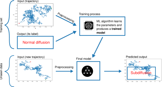
Figure 1: Workflow of our classification method. The training set is composed of a large number of synthetic trajectories (Sec. V.2). The preprocessing phase consists in extraction of features introduced in Sec. VI.

In the preprocessing phase, the raw data is cleaned and transformed into a form required as input by the classifier. Many traditional classifiers including random forest and gradient boosting work much better with vectors of features characterizing each trajectory instead of raw data. The features used in this work are introduced in Sec. VI. Some authors normalize the trajectories before further processing Muñoz-Gil et al. (2020). However, we omitted this step as our preliminary analysis indicated a significant decrease in the performance of the classifiers induced by normalization. The ensembles of trees were inferred from the feature vectors and their labels. Once trained, they may be used to classify new trajectories, including the experimental ones.

IV Stochastic models of diffusion

The most popular theoretical models of diffusion commonly employed are: continuous-time random walk (CTRW) Metzler and Klafter (2000), obstructed diffusion (OD) Havlin and Ben-Avraham (1987); Saxton (1994), random walk on random walks (RWRW) Blondel et al. (2019), random walks on percolating clusters (RWPC) Straley (1980); Metzler et al. (2014) fractional Brownian motion (FBM) Mandelbrot and Ness (1968); Guigas et al. (2007); Burnecki et al. (2012), fractional Levy $\alpha$-stable motion (FLSM) Burnecki and Weron (2010), fractional Langevin equation (FLE) Kou and Xie (2004) and autoregressive fractionally integrated moving average (ARFIMA) Burnecki and Weron (2014). They are applicable to different physical environments: trapping and crowded environments (CTRW, FFPE); labyrinthine environments (OD, RWPC, RWRW); viscoelastic systems (FBM, FLSM, FLE, ARFIMA); systems with time-dependent diffusion (scaled FBM, ARFIMA). Following Refs. Briane et al. (2018); Weron et al. (2019), we will focus on three stochastic processes known to generate different kinds of fractional diffusion: fractional Brownian motion, directed Brownian motion (DBM) Elston (2000) and Ornstein-Uhlenbeck process (OU) MacLeod et al. (2010).

FBM is the solution of the stochastic differential equation

$$dX_{t}^{i}=\sigma dB_{t}^{H,i},~{}~{}i=1,2,$$ (6)

where the parameter $\sigma>0$ relates to the diffusion coefficient via $\sigma=\sqrt{2D}$, $H$ is the Hurst parameter ($H=\alpha/2$) and $B_{t}^{H}$ - a continuous-time Gaussian process that starts at zero, has expectation zero and has the following covariance function:

$$\mathrm{E}\left(B^{H}_{t}B^{H}_{s}\right)=\frac{1}{2}\left(|t|^{2H}+|s|^{2H}-|t-s|^{2H}\right).$$ (7)

For $H<\frac{1}{2}$ (i.e. $\alpha<1$), FBM produces subdiffusive trajectories. It corresponds to a scenario, in which a particle is hindered by mobile or immobile obstacles Jeon et al. (2011). It reduces to the free diffusion at $H=\frac{1}{2}$. And for $H>\frac{1}{2}$, FBM generates superdiffusive motion (Fig. 2a).

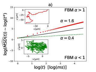
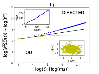
Figure 2: Time-averaged mean-squared displacement calculated for: (a) FBM with different values of $\alpha$, (b) DBM and OU processes. The trajectories used to calculate the MSD curves are shown in the corresponding insets and are consistent with real data time and distance scales: $ms$ and $\mu m$ accordingly. The solid line in both plots indicates TAMSD of normal diffusion.

The directed Brownian motion, also known as the diffusion with drift, is the solution to

$$dX_{t}^{i}=v_{i}dt+\sigma dB_{t}^{1/2,i},~{}~{}i=1,2,$$ (8)

where $v=(v_{1},v_{2})\in\mathbf{R}^{2}$ is the drift parameter. This process generates superdiffusion related to an active transport of particles driven by molecular motors. The velocity of the motors is modeled by the parameter $v$ (Fig. 2b). For $v=0$, the process reduces to normal diffusion.

The Ornstein-Uhlenbeck process is known to model confined diffusion, which is a subclass of subdiffusion (Fig. 2b). It corresponds to a particle inside a potential well and is a solution to the following stochastic differential equation:

$$dX_{t}^{i}=-\lambda_{i}(X_{t}^{i}-\theta_{i})dt+\sigma dB_{t}^{1/2,i},~{}~{}i=1,2,~{}~{}\theta_{i}\in\mathbf{R}.$$ (9)

Here, $\theta=(\theta_{1},\theta_{2})$ is the equilibrium position of the particle and $\lambda_{i}$ measures the strength of interaction. For $\lambda_{i}=0$, OU reduces to normal diffusion as well.

V Our dataset

V.1 Real SPT data

The classifiers built in this study will be applied to the data from single-particle tracking experiment on G protein-coupled receptors and G proteins, already analyzed in Refs. Sungkaworn et al. (2017); Weron et al. (2019). The receptors are of great interest, because they mediate the biological effects of many hormones and neourotransmitters and are also important as pharmacological targets Pierce et al. (2002). Their signals are transmitted to the cell interior via interactions with G proteins. The analysis of the dynamics of these two types of molecules will shed more light on how the receptors and G proteins meet, interact and couple.

A subset of that data has been already studied by means of statistical methods in Ref. Weron et al. (2019). Since we are interested in using those results as a benchmark for our classifiers, we will focus on the very same subset of data in our analysis. Hence, only trajectories with at least 50 steps will be taken into account, resulting in 1037 G proteins and 1218 receptors. The trajectories under consideration for both types of molecules are visualized in Fig. 3.

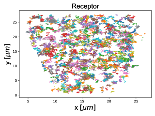
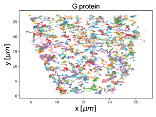
Figure 3: (Color online) Trajectories of the receptors (left) and G proteins (right) used as input for the classifiers. Different colors are introduced to indicate different trajectories. The set of the receptors contains $1218$ trajectories and the one of G proteins – $1037$ trajectories. The lengths of the trajectories are from range $[50,401]$, the time step is equal to $28.4$ ms, and recorded positions are given in $\mu\text{m}$.

V.2 Synthetic data

Building a classifier requires training data, which consists of a set of training examples Raschka (2015). Each of these examples is a pair of an input (trajectory) and its output label (diffusion type). In an optimal scenario the training set would contain real trajectories with their true labels from e.g. previous experiments on the same type of cells. However, collecting a training set consisting of real trajectories is practically impossible. First of all, independently of the method used for analysis, the labels of such trajectories are affected by some uncertainties Weron et al. (2019). Moreover, typical machine learning algorithms require thousands of training examples to provide a reasonable function that maps an input to an output and can be used for classification of new input data. That is why one usually resorts to synthetic, computer generated trajectories to prepare the training set. In this case the true label of each trajectory is known in advance and it is rather cheap to generate many of them.

The stochastic processes described in Sec. IV will be used to generate the training set. Just to recall, a discrete trajectory of a particle is given by

$$X_{n}=\left(X_{t_{0}},X_{t_{1}},\dots,X_{t_{N}}\right),$$ (10)

where $X_{t_{i}}=\left(X^{1}_{t_{i}},X^{2}_{t_{i}}\right)\in\mathbf{R}^{2}$ is the position of the particle at time $t_{i}=t_{0}+i\Delta t$, $i=0,1,\dots,N$. The lag $\Delta t$ between two consecutive observations is assumed to be constant. In tracking experiments, it is determined by the temporal resolution of the imaging method. However, we will assume the lag being equal to $1\,s$ in the simulations. Similarly, we will use $\sigma=1\,\mu m\,s^{-1/2}$ most of the time (see Sec. V.4 for an exception to this choice). In total, $120000$ trajectories have been generated for the main training set. Their length was randomly chosen from the range between 50 and 500 steps. No additional noise was added to the raw data in this set (see Sec. V.3 for a set with noise).

A summary of the training set is presented in Table 1. The case of the free diffusion requires probably a short explanation. From the description in Sec. IV we know that all of the models reduce to the normal Brownian motion for some specific values of the parametres ($H=0.5$ for FBM, $v=0$ for DBM and $\lambda=0$ for OU). However, it is very difficult to distinguish anomalous diffusion processes from the normal one already if their parameters are in the vicinity of those values. That is why we extended the ranges of parameter values corresponding to the free diffusion. Although introduced here at a different level, this approach resembles the cutoff $c$ used in Ref. Weron et al. (2019) to classify the results. As for the value, we take the smallest one considered therein.

Type of diffusion	Model	Parameter ranges	# of trajectories
Normal diffusion	FBM	$H\in[0.5-c,0.5+c]$	20000
	DBM	$v\in[0,c]$	10000
	OU	$\theta=0,\lambda=[0,c]$	10000
Subdiffusion	FBM	$H\in[0.1,0.5-c)$	20000
	OU	$\theta=0,\lambda=(c,1]$	20000
Superdiffusion	FBM	$H\in(0.5+c,0.9]$	20000
	DBM	$v\in(c,1]$	20000

Table 1: Summary of the synthetic trajectories used as the training set. The parameter $c$ was set to 0.1 in all simulations. If not specified otherwise, $\sigma=1\,\mu m\,s^{-1/2}$ and $\Delta t=1\,s$ were used.

The Python package fbm Flynn (17 ) was used to simulate the FBM trajectories as well as the Brownian motion part of the diffusion with drift. By default, the fbm() function from that package utilizes the Davies-Harte method Davies and Harte (1987) for fastest performance. However, the method is known to fail for the Hurst parameter close to 1. If this occurs, the function fallbacks to the Hosking’s algorithm Hosking (1984). The OU process was generated with the OrnsteinUhlenbeckProcess object from the stochastic package Flynn (18 ). This object uses the Euler-Maruyama method Kloeden and Platen (1992) to produce realizations of the process.

V.3 Adding noise

The synthetic dataset introduced in the previous section constitutes our main training set for building the classifiers. For the sake of comparison with statistical methods presented in Ref. Weron et al. (2019), it consists of pure trajectories, that do not suffer from any localization errors.

However, real data is usually affected by different kinds of noise. For instance, slow drift currents in the cytoplasm may induce low frequency noise. Typically, it may be reduced by various detrending methods Michalet (2010); Mellnik et al. (2016). In contrast, high frequency noise can be due to a variety of reasons: mechanical vibrations of the instrumental setup; particle displacement while the camera shutter is open; noisy estimation of true position from the pixelated microscopy image; error-prone tracking of particle positions when they are out of the camera focal plane Deschout et al. (2014); Weiss (2013); Burnecki et al. (2015); Calderon (2016); Weiss (2019).

To account for different localization errors and to check their impact on the performance of the classifiers, we prepared a second training set by simply adding a normal Gaussian noise with zero mean and standard deviation $\sigma_{gn}$ to each simulated trajectory. We followed the procedure already used in Refs. Wagner et al. (2017); Kowalek et al. (2019). That means, instead of setting $\sigma_{gn}$ directly, we first introduced the signal to noise ratio,

$$Q=\left\{\begin{array}[]{cc}\frac{\sqrt{D\Delta t+v^{2}\Delta t^{2}}}{\sigma_{gn}}&{\rm for~{}DBM},\\ \frac{\sqrt{D\Delta t}}{\sigma_{gn}}&{\rm otherwise},\end{array}\right.$$ (11)

where $v=\sqrt{v_{1}^{2}+v_{2}^{2}}$. For each trajectory, $Q$ was randomly set in the range from 1 (high noise) to 9 (low one). Then, Eq. (11) was used to determine $\sigma_{gn}$ for given $D$ and $\Delta t$.

V.4 Auxiliary training set

During our first attempt to apply the classifiers to experimental data it turned out that the parameter $\sigma=1$, taken from Ref. Weron et al. (2019), may not be the best choice for real trajectories under investigation. Thus, we also prepared an auxiliary training set of synthetic trajectories, which were simulated with no noise and $\sigma=0.38$. This particular value of $\sigma$ corresponds to the diffusion coefficient $D=0.0715\,\mu m^{2}\,s^{-1}$ and will be explained in Sec. VII.5.3. All other parameters of the set are exactly the same as in the main training set introduced in Sec. V.2.

VI Classification features

The random forest and gradient boosting algorithms require human-engineered features representing the trajectories for both the model training and the classification of new data. Choosing the right features constitutes a challenge and is crucial for the classification results. For instance, in Ref. Kowalek et al. (2019) we considered a set of features proposed for the first time by Wagner et al Wagner et al. (2017). Although we did not apply them to real data, we showed that classifiers using those features do not generalize well to data generated with models different from the ones used for training.

A more detailed discussion on the role of the features will be addressed in a forthcoming paper. In this work we use a new set of features motivated by the statistical analysis carried out in Ref. Weron et al. (2019). The main conclusion of that paper was that, even though statistical methods going beyond the standard MSD classification may provide good results even for short trajectories, no method was found to be superior in all examples and one should actually combine different approaches to get reliable results.

Following this recommendation, we decided to extract features from all methods considered in Ref. Weron et al. (2019) and to use them simultaneously as the input for our classifiers. Thus, our feature set will consist of:

• anomalous $\alpha$ exponent (fitted to TAMSD),

• the diffusion coefficient $D$ (fitted to TAMSD),

• the standarized value

  $$T_{N}=\frac{D_{N}}{\sqrt{\hat{\sigma}_{N}^{2}(t_{N}-t_{0})}}$$ (12)

  of the maximum distance $D_{N}$ traveled by a particle,

  $$D_{N}=\max_{i=1,2,\dots,N}\|X_{t_{i}}-X_{t_{0}}\|,$$ (13)

  where $\hat{\sigma}_{N}$ is a consistent estimator of the standard deviation of $D_{N}$,

  $$\hat{\sigma}_{N}^{2}=\frac{1}{2N\Delta t}\sum^{N}_{j=1}\|X_{t_{j}}-X_{t_{j-1}}\|^{2}_{2},$$ (14)

• the power $\gamma^{p}$ (in the function $kn^{\gamma^{p}}$) fitted to $p$-variation Magdziarz et al. (2009); Burnecki and Weron (2010)

  $$\hat{V}_{n}^{(p)}=\sum_{k=0}^{N/n-1}\|X_{(k+1)n}-X_{kn}\|^{p}$$ (15)

  for values of $p$ from 1 to 5.

Note that the first two of the above features were included in the feature set used in Refs. Kowalek et al. (2019). To determine their values, the maximum lag equal to 10% of each trajectory’s length was used to calculate the corresponding TAMSD curve.

VII Results

We used the scikit-learn Pedregosa et al. (2011) implementations of the random forest and gradient boosting algorithms. As already stated in Ref. Kowalek et al. (2019), a cluster of 24 CPUs with 25 GB total memory was used to perform the computation. The processing time (feature extraction, hyperparameter tuning, training and validation of a model) was of the order of two hours in each case. If not stated otherwise, the dataset without noise (see Sec. V.2) was used to train the classifiers.

VII.1 Details of the classifiers

In order to find optimal models, we used the RandomisedSearchCV method from scikit-learn library. It allows to perform a search over a grid of hyperparameter ranges. Here, a hyperparameter of the model is understood as a parameter, whose value is set before the learning process begins (it cannot be derived simply by training of the model).

In Table. 2, the optimal values of the hyperparameters for our training set are listed. The “with $D$” column in the table refers to the full set of features defined in Sec. VI. The “no $D$” columns corresponds to a reduced feature set with the diffusion coefficient $D$ removed from consideration. The reason for introducing the latter set will be explained in Sec. VII.5.

	Random forest		Gradient boosting
	with $D$	no $D$	with $D$	no $D$
bootstrap	$True$	$True$	NA	NA
criterion	$entropy$	$entropy$	NA	NA
max_depth	60	10	10	10
max_features	$log_{2}$	$sqrt$	$log_{2}$	$log_{2}$
min_samples_leaf	4	2	2	2
min_samples_split	2	10	2	2
n_estimators	900	600	100	100

Table 2: Hyperparameters of the optimal classifiers found with both methods. Their meaning is explained in Sec. VII.1. The “with $D$” column refers to the full feature set, “no $D$” one - to the feature set after removal of the diffusion coefficient $D$. $NA$ stands for “Not Applicable” (the first two parameters are random forest specific).

The bootstrap hyperparameter is a boolean value. It decides whether bootstrap samples ($True$) or the whole data set ($False$) are used to build each single tree. Criterion specifies, which function should be used to measure the quality of a split of data into subsamples at a new node of the tree. Gini impurity and information entropy are available for that purpose Raschka (2015). The max_depth is the maximum depth (the number of levels) of each decision tree. The number of features to consider when looking for the best split is given by max_features. If equal to log2 (sqrt), then the number is calculated as the logarithm (square root) of the number of features. Min_samples_split specifies the minimum number of samples required to split a subset of data at an internal node of the tree. Min_samples_leaf is the minimum number of samples required to be at a leaf node (a node representing a class label). Finally, n_estimators gives the number of trees in the ensemble.

As it follows from Table 2, the ensemble found with gradient boosting is significantly smaller than the one generated with the random forest method.

VII.2 Performance of the classifiers

Since our synthetic data set is perfectly balanced (same number of trajectories in each class), we may start the analysis of the classifiers simply by looking at their accuracy. It is one of the basic measures to assess the classification performance, defined as the number of correct predictions divided by the total number of preditions.

From the results listed in Table 3 it follows that in the case of the training set, the gradient boosting method is the more accurate one, even though the differences are small. Moreover, its decline in accuracy after the removal of $D$ from the feature set is smaller than for random forest. However, the latter one performs a little bit better on the test set, indicating a small tendency of GB to overfit. Despite these differences, both classifiers perform very well.

	Random forest		Gradient boosting
Data set	with $D$	no $D$	with $D$	no $D$
Training	0.977	0.953	0.992	0.989
Test	0.948	0.946	0.947	0.944

Table 3: Accuracies of the optimal classifiers for both the training and the test data.

The normalized confusion matrices of the classifiers are presented in Fig. 4. By definition, an element $C_{ij}$ of the confusion matrix is equal to the number of observations known to be in class $i$ (true labels) and predicted to be in class $j$ (predicted labels) Raschka (2015). In all cases, the worst performance (93% of correctly predicted labels) is observed for the normal diffusion. This relates probably to the fact that in our synthetic training set we also tagged anomalous trajectories with parameters slightly deviating from the normal ones as free diffusion.

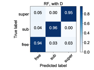
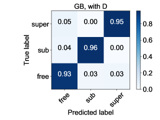
Figure 4: Normalized confusion matrices for random forest and gradient boosting classifiers. The “with $D$” label refers to the full feature set, “no $D$” one - to the feature set after removal of the diffusion coefficient $D$. All results are rounded to two decimal digits.

The data collected in Fig. 4 may be used to calculate some other popular measures giving more insight into the performance of the classifiers: precision, recall and F1 score Perry et al. (1955). Precision is the fraction of correct predictions of a class among all predictions of that class. It tells us how often a classifier is correct if it predicts a given class. Recall is the fraction of correct predictions of a given class over the total number of members of that class. It measures the number of relevant results within a predicted class. A harmonic mean of precision and recall gives the F1 score - another measure of classifier’s accuracy.

As we see from Table 4, both models return much more relevant results than the irrelevant ones (high precision). Moreover, they yield most of the relevant results (high recall). The F1 scores resemble the accuracies given in Table 3.

Method	Features	Measure	Normal diffusion	Subdiffusion	Superdiffusion	Total/Average
		Support	12000	12000	12000	36000
		Precision	0.912	0.969	0.966	0.949
	with $D$	Recall	0.935	0.958	0.951	0.948
RF		F1	0.923	0.963	0.959	0.948
		Support	12000	12000	12000	36000
	no $D$	Precision	0.908	0.967	0.967	0.947
		Recall	0.935	0.955	0.950	0.947
		F1	0.921	0.961	0.958	0.947
		Support	12000	12000	12000	36000
		Precision	0.911	0.967	0.965	0.948
	with $D$	Recall	0.933	0.958	0.951	0.947
GB		F1	0.922	0.962	0.958	0.947
		Support	12000	12000	12000	36000
	no $D$	Precision	0.907	0.963	0.964	0.945
		Recall	0.928	0.954	0.951	0.944
		F1	0.917	0.958	0.957	0.944

Table 4: Detailed performance analysis of both classification methods on the test data. Support is the number of trajectories known to belong to a given class. All results are rounded to two decimal digits.

VII.3 Feature importances

While working with the human-engineered features, it may happen that some of them are more informative than the others. Therefore, knowing the relative importances of the features is useful, because it can provide further insight into the data and the classification model. The features with high importances are the drivers of the outcome. The least important ones might often be omitted from the model, making it faster to fit and predict. The latter is of particular significance in case of models with very large feature sets, as it may additionally help to reduce the dimensionality of the problem.

There are several ways to determine the feature importances. The one implemented in the scikit-learn library is defined as the total decrease in node impurity caused by a given feature, averaged over all trees in the ensemble Breiman et al. (1984). In other words, the Gini impurities (4) are calculated before and after each split on a given feature to determine the total decrease in the impurity related to that feature. The outcome is then averaged over all trees in the ensemble.

Relative feature importances for both classifiers are shown in Table 5. The features are ordered according to the descending scores in case of the random forest with $D$.

	Random forest		Gradient boosting
Feature	with $D$	no $D$	with $D$	no $D$
$2$-var	0.296	0.239	0.238	0.160
$\alpha$	0.201	0.197	0.274	0.125
$3$-var	0.178	0.183	0.108	0.245
$1$-var	0.171	0.200	0.204	0.210
$4$-var	0.078	0.110	0.095	0.145
$T_{N}$	0.038	0.032	0.030	0.037
$5$-var	0.022	0.038	0.034	0.077
$D$	0.017	–	0.016	–

Table 5: Feature importances for both methods, sorted in the descending order of the scores in case of random forest with $D$. The bold face indicates the most important features in each case. The least important ones are underlined. The “with $D$” label refers to the full feature set, “no $D$” one - to the feature set after removal of the diffusion coefficient $D$.

We see that the $p$-variation for $p=2$ ($2$-var) is the most informative feature, followed by the anomalous exponent $\alpha$. The diffusion coefficient is the least important feature. After its removal the relative importances of the remaining features changed. The differences between them are smaller now. Moreover, the $1$-var became the second most important attribute and $T_{N}$ - the least important one.

Gradient boosting differs slightly from the random forest. In case with $D$, the order of the top two features is reversed. After removal of $D$, $3$-var and $1$-var became the most informative ones. The exponent $\alpha$ lost much of its importance. And again, $T_{N}$ is the least informative attribute.

VII.4 Note on auxiliary classifiers

Apart from the main collection of synthetic trajectories described in Sec. V.2, we generated two additional training sets. The first one was built from the main set by simply adding noise (Sec. V.3) and the second one – with a smaller value (0.38 vs 1) of the parameter $\sigma$ (Sec. V.4).

Those sets were then used to train new classifiers. Their accuracies are listed in Table 6.

	Random forest		Gradient boosting
Data set	with $D$	no $D$	with $D$	no $D$
with noise	0.946	0.932	0.946	0.930
with $\sigma=0.38$	0.953	0.950	0.952	0.950

Table 6: Accuracies of the classifiers trained on auxiliary data sets: the first with noise (see Sec. V.3) and the second with $\sigma=0.38$ (Sec. V.4) ).

Note that those values are very similar to the ones presented in Table 3. Thus, all classifiers perform very well on their corresponding synthetic test sets. Interestingly, the machine learning algorithms seem to deal excellent with noisy data, as there is no significant drop in the accuracy of the classifiers trained on that data.

The basic characteristics of the additional classifiers turned out to be practically indistinguishable from the ones presented in the previous sections. Thus, we will skip their detailed description for the sake of readability.

VII.5 Application to real data

VII.5.1 Summary of statistical methods

In Table 7, classification results from Ref. Weron et al. (2019) for the G protein-coupled receptors and G proteins (see Sec. V.1 for details) are summarized.

	MSD		MSD test		MAX		1-var		2-var
	R	G	R	G	R	G	R	G	R	G
Normal diffusion	19%	22%	79%	76%	79%	76%	53%	52%	47%	51%
Subdiffusion	80%	72%	21%	24%	21%	24%	47%	46%	53%	48%
Superdiffusion	1%	6%	0 %	1%	0%	1%	0%	1%	0%	2%

Table 7: Summary of the classification results from Ref. Weron et al. (2019). Columns labeled with R and G correspond to the G protein-coupled receptors and G proteins, respectively. The MSD data was calculated for $c=0.1$ (see Sec. V.2 for explanation) and the maximum lag equal to 10% of the trajectories’ lengths. Due to rounding, the numbers may not add up precisely to 100%.

Except the standard MSD method, the authors used statistical testing procedures based on: (a) MSD (referred as “MSD test” in Table 7), (b) maximum distance traveled by a particle (“MAX”) and (c) $p$-variations at different values of $p$ (“1-var” and “2-var”). As wee see, the methods do not yield coherent results. MSD classifies most of the trajectories as subdiffusion. The MAX and MSD test procedures indicate a prevalence of freely diffusing particles in the same data set. The $p$-var tests give similar proportions of normal and subdiffusive trajectories. Moreover, only the standard MSD method is able to recognize a noticeable subset of trajectories as superdiffusion. Further analysis with synthetic data revealed that the $p$-var method is the most accurate one for FBM, while the MSD/MAX tests are the best choice (in terms of errors) for OU and DBM processes.

VII.5.2 Classification with full feature set

Our first attempt to classify the data with the whole feature set defined in Sec. VI is presented in Table 8.

	Random forest		Gradient boosting
	Receptor	G protein	Receptor	G protein
Normal diffusion	38%	44%	38%	38%
Subdiffusion	61%	54%	60%	55%
Superdiffusion	0%	1%	0%	5%

Table 8: Diffusion modes of real trajectories found with classifiers trained on the main synthetic dataset ($\sigma=1$, no noise; see Sec. V.2) with the full set of features (referred to as “with D” in the previous sections). Due to rounding, the numbers may not add up precisely to 100%.

As we see, both methods work similarly, with gradient boosting recognizing more G protein trajectories as a superdiffusive motion. Most of the trajectories are classified as normal or subdiffusion, with the prevalence of the latter. Note that the numbers given in Table 8 do not match any of the results generated with the statistical methods. Thus, it is really hard to judge which method should be chosen to work with real data.

VII.5.3 Role of $D$ and classification with reduced feature set

To pin down a possible cause for the deviation from the statistical methods, let us have a look at the distribution of values of the generalized diffusion coefficient $D$ among the trajectories in the real data set. The corresponding histograms for the G protein-coupled receptors and G proteins are shown in Fig. 5.

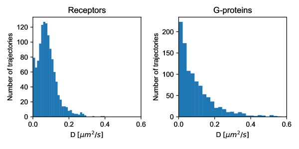
Figure 5: Distribution of $D$ among trajectories in the real data set.

To calculate the histograms, $D$ was simply extracted from the MSD curves under the assumption of the anomalous diffusion model Weron et al. (2019). Its values in the data set turned out to be much smaller than in the synthetic data set, with $D=0.0715$ being the most frequent one. However, the synthetic training set was generated with $\sigma=1$ (i.e. $D=0.5$) for all types of diffusion. Thus, the discrepancy in the classification results from any of the methods presented in Weron et al. (2019) may simple be caused by the fact, that the classifiers were trained for a different regime of diffusion.

To check this hypothesis let us classify the trajectories with the models trained on the data set generated with $\sigma=0.38$, which corresponds to $D=0.0715$. Classification results with the full set of features are presented in Table 9.

	Random forest		Gradient boosting
	Receptor	G protein	Receptor	G protein
Normal diffusion	54%	51%	54%	51%
Subdiffusion	45%	47%	45%	46%
Superdiffusion	0%	1%	0%	1%

Table 9: Diffusion types found in real data with the classifiers trained on the auxiliary dataset ($\sigma=0.38$, no noise; see Sec. V.4) with the full set of features (referred to as “with D” in the previous sections). Due to rounding, the numbers may not add up precisely to 100%.

The results differ from the previous classification. Now, the shares of the trajectories are very similar to the ones obtained with $1$-var and $2$-var methods from Ref. Weron et al. (2019). Most of the trajectories belong either to the normal diffusion or the subdiffusion class, with the first having a slightly larger count. There is only a bunch of data samples recognized as superdiffusion in case of G proteins.

Treating the statistical results as a reference point, we can indeed say that adjusting $\sigma$ to the real data set improved the results. However, this procedure is not really convenient, as it requires generation of a new synthetic data set, extracting of features and training of a new classifier practically every time new experimental samples are arriving.

In search of a more universal procedure we decided to train new classifiers on the reduced set of features not containing the diffusion coefficient $D$, but we used the main synthetic set with $\sigma=1$ as in Ref. Weron et al. (2019). Since $D$ turned out to be the least informative feature (Table 5), it was the natural candidate for the removal anyway. We know already, that the accuracy of the classifiers without $D$ is a little bit smaller (Table 3). Nevertheless, we expect them to work better on unseen data. Indeed, even though the choice of $\sigma$ was not optimal, the classification results shown in Table 10 resemble the ones obtained above (Table 9) and the $1$-var and $2$-var methods from Ref. Weron et al. (2019).

	Random forest		Gradient boosting
	Receptor	G protein	Receptor	G protein
Normal diffusion	52%	53%	56%	54%
Subdiffusion	46%	45%	43%	43%
Superdiffusion	0%	1%	0%	1%

Table 10: Results of classifiers trained on the main synthetic dataset ($\sigma=1$, no noise) with the reduced set of features, after removal of $D$ (referred to as “no D” in the previous sections). Due to rounding, the numbers may not add up precisely to 100%.

Again, most of the trajectories belong either to the normal diffusion or the subdiffusion class, with the first having a larger count. Just few data samples are recognized as superdiffusion in case of G proteins.

The advantage of the classification with the reduced data set over the one with the adjustment of $\sigma$ lies in that the classifier is trained only once and then may be simply applied to any unseen samples. It does not require a recurring and time consuming procedure of adjustment of $\sigma$, generation of tailor-made training data, extraction of features and training of the classifier every time a new set of experimental trajectories is arriving for analysis.

The agreement with the $p$-variation procedure for small values of $p$ makes perfect sense, if we recall that $2$-var and $1$-var belong to be the most informative among the features used by the classifiers to distinguish between the data samples.

VII.5.4 Impact of noise

Although it goes beyond a comparison of machine learning algorithms with the statistical methods from Ref. Weron et al. (2019), as its authors used only pure trajectories, we would like to conclude this section by applying the classifier trained on noisy data (Sec. V.3) to the real trajectories. Results of classification with the reduced feature set are shown in Table 11.

	Random forest		Gradient boosting
	Receptor	G protein	Receptor	G protein
Normal diffusion	62%	58%	63%	58%
Subdiffusion	38%	40%	36%	40%
Superdiffusion	0%	2%	0%	3%

Table 11: Results of classifiers trained on noisy data ($\sigma=1$) with the reduced set of features (referred to as “no D” in the previous sections). Due to rounding, the numbers may not add up precisely to 100%.

The introduction of noise has changed the results. Although still most of the trajectories belong either to the normal diffusion or to the subdiffusion class, the first has now larger count compared with the case without noise in the synthetic data. As we already pointed out in Sec. V.2, the boundary between the normal and anomalous modes in the vicinity of $\alpha=1$ is not particularly well defined even in the absence of noise. This boundary is further blurred in the presence of noise, resulting in the observed rearrangement of class memberships. However, if we still would like to relate the “noisy” results with the ones from Ref. Weron et al. (2019), they are close to an average of $1$-var and $MAX$ methods.

VIII Discussion

Machine learning methods used for classification of SPT data are known to sometimes fail to generalize to unseen data Kowalek et al. (2019). In this paper, we revisited our ML approach to trajectory classification and presented a new set of features, which are required by the classifiers to process the input data. This new set allows the random forest and gradient boosting classifiers to transfer the knowledge from a synthetic training set to real data. The classifiers were tested on a subset of experimental data describing G proteins and G protein-coupled receptors Sungkaworn et al. (2017). The results were then compared to four statistical testing procedures introduced in Ref. Weron et al. (2019).

We have shown that the choice of the feature set is crucial, as even a small change in its content may significantly impact the behavior of the classifiers. We decided to use a set consisting of the anomalous $\alpha$ exponent, the diffusion coefficient $D$, the maximum distance traveled by a particle, the power $\gamma^{p}$ fitted to $p$-variation for values of $p$ from 1 to 5. These features were extracted from several statistical methods presented in Ref. Weron et al. (2019). Since none of the methods turned out to be superior to the others, the authors of the work proposed to take a mean of the results of all methods in order to minimize the risk of large errors. Due to the fact that our classifiers use all features simultaneously as input, in some sense we followed their advice. From our findings it follows that with the full feature set, the machine learning methods applied to the real data yield results completely different from the ones produced with the statistical methods. However, adjusting the diffusion coefficient in the synthetic trajectories to the most frequent value among the real samples or removing this coefficient from the feature set and re-training the classifiers starts to produce results very similar to the $p$-variation method from Ref. Weron et al. (2019).

From the above methods, the one with the reduced set of features is more convenient, because the classifier is trained only once and then may be simply applied to any unseen data. It does not require a recurring and time consuming procedure consisting of: (1) adjustment of $\sigma$, (2) generation of tailor-made training data, (3) extraction of features and (4) training of the classifier every time a new set of experimental trajectories is arriving for analysis.

The agreement between the ML approach and the statistical testing based on $p$ variations is, on one hand, a confirmation that our ML methods are able to classify unseen data in a reasonable way. On the other hand, it may support the choice of the $p$-variation testing procedure among the statistical methods.

Introduction of noise mimicking different kinds of localization errors changed the classification results – the count of normal diffusion (subdiffusion) trajectories increased (decreased) by a couple of percentage points. A slight increase of superdiffusion samples was also observed in case of G proteins. If we would like to relate the “noisy” results with the ones from Ref. Weron et al. (2019), they are close to an average of $1$-var and $MAX$ methods.

Although still a lot needs to be done in terms of selection of robust features and the generation of appropriate synthetic training data, we believe that our methodology may be successfully applied to experimental data in order to provide a further insight into the dynamics of complex biological processes.

*

Appendix A Codes

Python codes for every stage of the classification procedure shown in Fig. 1, together with a short documentation, are publicly available at Zenodo (see Ref. Janczura et al. (2020)).

References

- Barak and Webb (1982) L. Barak and W. Webb, Journal of Cell Biology 95, 846 (1982), https://rupress.org/jcb/article-pdf/95/3/846/459484/846.pdf .
- Kusumi et al. (1993) A. Kusumi, Y. Sako, and M. Yamamoto, Biophysical Journal 65, 2021 (1993).
- Yildiz et al. (2003) A. Yildiz, J. N. Forkey, S. A. McKinney, T. Ha, Y. E. Goldman, and P. R. Selvin, Science 300, 2061 (2003).
- Kural et al. (2005) C. Kural, H. Kim, S. Syed, G. Goshima, V. I. Gelfand, and P. R. Selvin, Science 308, 1469 (2005).
- Izeddin et al. (2014) I. Izeddin, V. Récamier, L. Bosanac, I. I. Cissé, L. Boudarene, C. Dugast-Darzacq, F. Proux, O. Bénichou, R. Voituriez, O. Bensaude, M. Dahan, and X. Darzacq, eLife 3, e02230 (2014).
- Gal et al. (2013) N. Gal, D. Lechtman-Goldstein, and D. Weihs, Rheologica Acta 52, 425 (2013).
- Bressloff (2014) P. C. Bressloff, Stochastic processes in cell biology, Interdisciplinary applied mathematics (Springer, Cham [u.a.], 2014) literaturverz. S. 645 - 672.
- Saxton (1994) M. J. Saxton, Biophysical Journal 67, 2110 (1994).
- Saxton and Jacobson (1997) M. J. Saxton and K. Jacobson, Annu. Rev. Biophys. Biomol. Struct. 26, 373 (1997).
- Feder et al. (1996) T. J. Feder, I. Brust-Mascher, J. P. Slattery, B. Baird, and W. W. Webb, Biophysical Journal 70, 2767 (1996).
- Metzler and Klafter (2000) R. Metzler and J. Klafter, Physics Reports 339, 1 (2000).
- Michalet (2010) X. Michalet, Physical Review E 82, 041914 (2010).
- Alves et al. (2016) S. B. Alves, G. F. O. Jr., L. C. Oliveira, T. P. de Silansa, M. Chevrollier, M. Oriá, and H. L. S. Cavalcante, Physica A 447, 392 (2016).
- Hoze et al. (2012) N. Hoze, D. Nair, E. Hosy, C. Sieben, S. Manley, A. Herrmann, J.-B. Sibarita, D. Choquet, and D. Holcman, Proceedings of the National Academy of Sciences 109, 17052 (2012), https://www.pnas.org/content/109/42/17052.full.pdf .
- Berry and Chaté (2014) H. Berry and H. Chaté, Phys. Rev. E 89, 022708 (2014).
- Weiss et al. (2004) M. Weiss, M. Elsner, F. Kartberg, and T. Nilsson, Biophysical Journal 87, 3518 (2004).
- Arcizet et al. (2008) D. Arcizet, B. Meier, E. Sackmann, J. O. Rädler, and D. Heinrich, Phys. Rev. Lett. 101, 248103 (2008).
- Monnier et al. (2012) N. Monnier, S.-M. Guo, M. Mori, J. He, P. Lénárt, and M. Bathe, Biophysical Journal 103, 616 (2012).
- Kepten et al. (2015) E. Kepten, A. Weron, G. Sikora, K. Burnecki, and Y. Garini, PLoS ONE 10(2), e0117722 (2015).
- Briane et al. (2018) V. Briane, C. Kervrann, and M. Vimond, Phys. Rev. E 97, 062121 (2018).
- Weiss (2019) M. Weiss, Phys. Rev. E 100, 042125 (2019).
- Saxton (1993) M. J. Saxton, Biophysical Journal 64, 1766 (1993).
- Valentine et al. (2001) M. T. Valentine, P. D. Kaplan, D. Thota, J. C. Crocker, T. Gisler, R. K. Prud’homme, M. Beck, and D. A. Weitz, Phys. Rev. E 64, 061506 (2001).
- Gal and Weihs (2010) N. Gal and D. Weihs, Phys. Rev. E 81, 020903 (2010).
- Grebenkov et al. (2013) D. S. Grebenkov, M. Vahabi, E. Bertseva, L. Forró, and S. Jeney, Phys. Rev. E 88, 040701 (2013).
- Fuliński (2017) A. Fuliński, Journal of Physics A: Mathematical and Theoretical 50, 054002 (2017).
- Raupach et al. (2007) C. Raupach, D. P. Zitterbart, C. T. Mierke, C. Metzner, F. A. Müller, and B. Fabry, Phys. Rev. E 76, 011918 (2007).
- Burov et al. (2013) S. Burov, S. M. A. Tabei, T. Huynh, M. P. Murrell, L. H. Philipson, S. A. Rice, M. L. Gardel, N. F. Scherer, and A. R. Dinner, Proceedings of the National Academy of Sciences 110, 19689 (2013).
- Tejedor et al. (2010) V. Tejedor, O. Bénichou, R. Voituriez, R. Jungmann, F. Simmel, C. Selhuber-Unkel, L. B. Oddershede, and R. Metzler, Biophysical Journal 98, 1364 (2010).
- Burnecki et al. (2015) K. Burnecki, E. Kepten, Y. Garini, G. Sikora, and A. Weron, Scientific Reports 5, 11306 (2015).
- Das et al. (2009) R. Das, C. W. Cairo, and D. Coombs, PLOS Computational Biology 5, 1 (2009).
- Slator et al. (2015) P. J. Slator, C. W. Cairo, and N. J. Burroughs, PLOS ONE 10, 1 (2015).
- Slator and Burroughs (2018) P. J. Slator and N. J. Burroughs, Biophysical Journal 115, 1741 (2018).
- Weron et al. (2019) A. Weron, J. Janczura, E. Boryczka, T. Sungkaworn, and D. Calebiro, Phys. Rev. E 99, 042149 (2019).
- Raschka (2015) S. Raschka, Python Machine Learning (Packt Publishing, 2015).
- Thapa et al. (2018) S. Thapa, M. A. Lomholt, J. Krog, A. G. Cherstvy, and R. Metzler, Phys. Chem. Chem. Phys. 20, 29018 (2018).
- Cherstvy et al. (2019) A. G. Cherstvy, S. Thapa, C. E. Wagner, and R. Metzler, Soft Matter 15, 2526 (2019).
- Wagner et al. (2017) T. Wagner, A. Kroll, C. R. Haramagatti, H.-G. Lipinski, and M. Wiemann, PLoS ONE 12(1), e0170165 (2017).
- Kowalek et al. (2019) P. Kowalek, H. Loch-Olszewska, and J. Szwabiński, Phys. Rev. E 100, 032410 (2019).
- Muñoz-Gil et al. (2020) G. Muñoz-Gil, M. A. Garcia-March, C. Manzo, J. D. Martín-Guerrero, and M. Lewenstein, New Journal of Physics 22, 013010 (2020).
- Dosset et al. (2016) P. Dosset, P. Rassam, L. Fernandez, C. Espenel, E. Rubinstein, E. Margeat, and P.-E. Milhiet, BMC Bioinformatics 17, 197 (2016).
- Granik et al. (2019) N. Granik, L. E. Weiss, E. Nehme, M. Levin, M. Chein, E. Perlson, Y. Roichman, and Y. Shechtman, Biophysical Journal 117, 185 (2019).
- Bo et al. (2019) S. Bo, F. Schmidt, R. Eichhorn, and G. Volpe, Phys. Rev. E 100, 010102 (2019).
- Han et al. (2020) D. Han, N. Korabel, R. Chen, M. Johnston, A. Gavrilova, V. J. Allan, S. Fedotov, and T. A. Waigh, eLife 9, e52224 (2020).
- Hatami et al. (2018) N. Hatami, Y. Gavet, and J. Debayle, in Proceedings of SPIE, Tenth International Conference on Machine Vision (ICMV 2017), edited by A. Verikas, P. Radeva, D. Nikolaev, and J. Zhou (2018) p. 10696.
- Mitchel (1997) T. Mitchel, Machine Learning (McGraw-Hill Professional, 1997).
- Sungkaworn et al. (2017) T. Sungkaworn, M.-L. Jobin, K. Burnecki, A. Weron, M. J. Lohse, and D. Calebiro, Nature 550, 543 (2017).
- Höfling and Franosch (2013) F. Höfling and T. Franosch, Reports on Progress in Physics 76, 046602 (2013).
- Szymanski and Weiss (2009) J. Szymanski and M. Weiss, Phys. Rev. Lett. 103, 038102 (2009).
- Jeon and Metzler (2010) J.-H. Jeon and R. Metzler, Phys. Rev. E 81, 021103 (2010).
- Weigel et al. (2011) A. V. Weigel, B. Simon, M. M. Tamkun, and D. Krapf, Proceedings of the National Academy of Sciences 108, 6438 (2011).
- Weigel et al. (2012) A. V. Weigel, S. Ragi, M. L. Reid, E. K. P. Chong, M. M. Tamkun, and D. Krapf, Phys. Rev. E 85, 041924 (2012).
- Hellmann et al. (2011) M. Hellmann, J. Klafter, D. W. Heermann, and M. Weiss, Journal of Physics: Condensed Matter 23, 234113 (2011).
- Sadegh et al. (2017) S. Sadegh, J. L. Higgins, P. C. Mannion, M. M. Tamkun, and D. Krapf, Phys. Rev. X 7, 011031 (2017).
- Qian et al. (1991) H. Qian, M. P. Sheetz, and E. L. Elson, Biophysical Journal 60, 910 (1991).
- Vega et al. (2018) A. R. Vega, S. A. Freeman, S. Grinstein, and K. Jaqaman, Biophysical Journal 114, 1018 (2018).
- Lanoiselée et al. (2018) Y. Lanoiselée, G. Sikora, A. Grzesiek, D. S. Grebenkov, and A. Wyłomańska, Phys. Rev. E 98, 062139 (2018).
- Ho (1995) T. K. Ho, in Proceedings of the Third International Conference on Document Analysis and Recognition - Volume 1 (IEEE Computer Society, 1995).
- Ho (1998) T. K. Ho, IEEE Transactions on Pattern Analysis and Machine Intelligence 20(8), 832 (1998).
- Schapire et al. (1998) R. E. Schapire, Y. Freund, P. Bartlett, and W. S. Lee, Annals of Statistics 26, 1651 (1998).
- Friedman (2002) J. H. Friedman, Comput. Stat. Data Anal. 38, 367 (2002).
- Song and LU (2015) Y.-Y. Song and Y. LU, Shanghai Archives of Psychiatry 27, 130 (2015).
- Shannon (1948) C. E. Shannon, Bell Syst. Tech. J. 27, 379 (1948).
- James et al. (2013) G. James, D. Witten, T. Hastie, and R. Tibshirani, An Introduction to Statistical Learning with Applications in R (Springer, New York, NY, 2013).
- Bramer (2013) M. Bramer, Principles of Data Mining, 2nd ed. (Springer Publishing Company, Incorporated, 2013).
- Havlin and Ben-Avraham (1987) S. Havlin and D. Ben-Avraham, Advances in Physics 36, 695 (1987).
- Blondel et al. (2019) O. Blondel, M. R. Hilário, R. S. dos Santos, V. Sidoravicius, and A. Teixeira, Electron. J. Probab. 24, 33 pp. (2019).
- Straley (1980) J. P. Straley, Journal of Physics C: Solid State Physics 13, 2991 (1980).
- Metzler et al. (2014) R. Metzler, J.-H. Jeon, A. G. Cherstvy, and E. Barkai, Phys. Chem. Chem. Phys. 16, 24128 (2014).
- Mandelbrot and Ness (1968) B. B. Mandelbrot and J. W. V. Ness, SIAM Review 10, 422 (1968).
- Guigas et al. (2007) G. Guigas, C. Kalla, and M. Weiss, Biophysical Journal 93, 316 (2007).
- Burnecki et al. (2012) K. Burnecki, E. Kepten, J. Janczura, I. Bronshtein, Y. Garini, and A. Weron, Biophysical Journal 103, 1839 (2012).
- Burnecki and Weron (2010) K. Burnecki and A. Weron, Physical Review E 82, 021130 (2010).
- Kou and Xie (2004) S. C. Kou and X. S. Xie, Phys. Rev. Lett. 93, 180603 (2004).
- Burnecki and Weron (2014) K. Burnecki and A. Weron, Journal of Statistical Mechanics: Theory and Experiment 2014, P10036 (2014).
- Elston (2000) T. C. Elston, Journal of Mathematical Biology 41, 189 (2000).
- MacLeod et al. (2010) C. L. MacLeod, Z. Ivezi, C. S. Kochanek, S. Kozłowski, B. Kelly, E. Bullock, A. Kimball, B. Sesar, D. Westman, K. Brooks, R. Gibson, A. C. Becker, and W. H. de Vries, Astrophysical Journal 721, 1014 (2010).
- Jeon et al. (2011) J.-H. Jeon, V. Tejedor, S. Burov, E. Barkai, C. Selhuber-Unkel, K. Berg-Sørensen, L. Oddershede, and R. Metzler, Phys. Rev. Lett. 106, 048103 (2011).
- Pierce et al. (2002) K. L. Pierce, R. T. Premont, and R. J. Lefkowitz, Nature Reviews Molecular Cell Biology 3, 639 (2002).
- Flynn (17 ) C. Flynn, “FBM: Exact methods for simulating fractional brownian motion (fbm) or fractional gaussian noise (fgn) in Python.” (2017–), [Online; accessed 21-02-2019], https://github.com/crflynn/fbm .
- Davies and Harte (1987) R. B. Davies and D. S. Harte, Biometrika 74, 95 (1987).
- Hosking (1984) J. Hosking, Water Resources Research 20, 1898 (1984).
- Flynn (18 ) C. Flynn, “Stochastic: a python package for generating realizations of stochastic processes.” (2018–), [Online; accessed 20-04-2020], https://github.com/crflynn/stochastic/ .
- Kloeden and Platen (1992) P. E. Kloeden and E. Platen, Numerical Solution of Stochastic Differential Equations (Springer-Verlag, Berlin, Heidelberg, 1992).
- Mellnik et al. (2016) J. W. R. Mellnik, M. Lysy, P. A. Vasquez, N. S. Pillai, D. B. Hill, J. Cribb, S. A. McKinley, and M. G. Forest, Journal of Rheology 60, 379 (2016).
- Deschout et al. (2014) H. Deschout, F. C. Zanacchi, M. Mlodzianoski, A. Diaspro, J. Bewersdorf, S. T. Hess, and K. Braeckmans, Nature Methods 11, 253 (2014).
- Weiss (2013) M. Weiss, Phys. Rev. E 88, 010101 (2013).
- Calderon (2016) C. P. Calderon, Phys. Rev. E 93, 053303 (2016).
- Magdziarz et al. (2009) M. Magdziarz, A. Weron, K. Burnecki, and J. Klafter, Phys. Rev. Lett. 103, 180602 (2009).
- Pedregosa et al. (2011) F. Pedregosa, G. Varoquaux, A. Gramfort, V. Michel, B. Thirion, O. Grisel, M. Blondel, P. Prettenhofer, R. Weiss, V. Dubourg, J. Vanderplas, A. Passos, D. Cournapeau, M. Brucher, M. Perrot, and E. Duchesnay, Journal of Machine Learning Research 12, 2825 (2011).
- Perry et al. (1955) J. W. Perry, A. Kent, and M. M. Berry, American Documentation 6, 242 (1955).
- Breiman et al. (1984) L. Breiman, J. H. Friedman, R. A. Olshen, and C. J. Stone, Classification and Regression Trees (Wadsworth and Brooks, Monterey, CA, 1984).
- Janczura et al. (2020) J. Janczura, P. Kowalek, H. Loch-Olszewska, J. Szwabiński, and A. Weron, “Trajectory generators and classificators for fractional anomalous diffusion classification,” (2020), https://doi.org/10.5281/zenodo.3933357 .