Dynamics in Varying vacuum Finsler-Randers Cosmology

Abstract

In the context of Finsler-Randers theory we consider, for the first time, the cosmological scenario of the varying vacuum. In particular, we assume the existence of a cosmological fluid source described by an ideal fluid and the varying vacuum terms. We determine the cosmological history of this model by performing a detailed study on the dynamics of the field equations. We determine the limit of General Relativity, while we find new eras in the cosmological history provided by the geometrodynamical terms provided by the Finsler-Randers theory.

I Introduction

Since the pioneering discovery of the accelerating expansion of our Universe Riess:1998cb ; Perlmutter:1998np ; Aghanim:2018eyx cosmology is now in the limelight of modern science. The physical mechanism able to explain this accelerating universe is one of the greatest challenges of modern physics. Within the realm of General Relativity (GR) this acceleration is easily accommodated by introducing a dark energy sector(DE) Copeland:2006wr characterized by negative pressure. The simplest DE model arises with the inclusion of a positive and time-independent cosmological constant, namely $\Lambda$, in the gravitational equations of GR Peebles:2002gy ; Padmanabhan:2002ji . The resulting cosmological scenario is widely known as the $\Lambda$-cosmology and this cosmological model is in agreement with a series of observational data, however it suffers from two mayor problems, for details see Weinberg:1988cp .

This naturally leads to think of several alternative $\Lambda$-cosmological models Copeland:2006wr to investigate the same issue. One of the simplest and natural generalizations of the $\Lambda$-cosmology is to introduce time dependence in the $\Lambda$ term, which leads to varying vacuum cosmologies. On the other hand, apart from the concept of DE physics, an alternative route to mimic this accelerating phase appears either due to the direct modifications of GR leading directly to modified gravitational theories Sotiriou:2008rp ; DeFelice:2010aj ; Clifton:2011jh ; Capozziello:2011et ; Nojiri:2017ncd or by introducing new gravitational theories completely different from GR, such as the teleparallel equivalent of GR (TEGR) Cai:2015emx .

The models arising from this latter approach are usually known as the geometric dark energy (GDE) models. Although both DE and GDE models have been widely studied and acknowledged in the literature, research over the last several years has indicated that despite a large number of models, none of them can be considered to be a completely healthy and viable model able to portray the dynamical evolution of the universe. Most notably though, the physical nature and evolution of both DE and GDE are still unknown even after substantial cosmological research. Thus, the debates in search of a perfect cosmological theory have been the central theme of modern cosmology at present times. The studies so far clearly justify that there are definitely no reasons to favor any particular cosmological theory or model, at least in light of the recent cosmological observations.

An interesting gravitational theory in the context of the present accelerating expansion is based on the introduction of Finsler geometry, which gives rise to a wider geometrical picture of the universe extending the traditional Riemannian geometry. In other words, one can recover the Riemannian geometry as a special case of the Finslerian geometry. Thus Finslerian geometry is expected to provide more insights on the dynamics and evolution of the observed universe, and as a consequence, the cosmology in Finslerian geometry gained significant attention in the scientific community (eg Perelman ; Minas ; Ikeda ; Kouretsis ; Hohman ; hohman2 ; Edwards ; Vacaru ; Caponio ; Gibbons ). In particular, the Finsler-Randers (FR) metric Randers and the induced cosmological model Stav07 ; StavFluids is of special interest since the field equations include an extra geometrical term that acts as a DE fluid. As we pointed out the (FR) cosmological model contains in each point two metric structures, one Riemannian and one Finslerian so it can be considered as a direction-dependent $(-y)$ motion of the Riemannian /FRW model with osculating structure.

In the present article we consider a very general dynamical picture of the universe in which a time-dependent cosmological term is present within the context of Finslerian geometry. The presence of a time dependent cosmological term, $\Lambda(t)$ actually inherits an interaction in the cosmic sector. These kind of models are widely accepted in the literature for their ability to describe various cosmological eras. The plan of the paper is as follows.

In Section II we briefly discuss the FR cosmology. The varying vacuum model is described in Section III where we present the field equations and the models of our analysis. Section IV includes the main material of this work. In particular we present the dynamical analysis and we determine the cosmological evolution for the models of our consideration. Finally, in Section V we discuss our results.

II Finsler-Randers theory: An overview

The origin of the FR model is based on the Finslerian geometry Stav07 ; StavFluids which is a natural generalization of the traditional Riemannian geometry and it has gained considerable attention in the cosmological community, see for instance 15 ; Bekenstein ; Mir ; Bao ; 13 ; Gibbons  for more details in this direction. In what follows we describe the basics of the Finslerian geometry.

As shown by Asanov Asa41 , the general action for the osculating Riemannian space-time of Einstein field equations is derived by a variational principle of the integral action, $\displaystyle I_{{}_{G}}=\int L\big{(}x,y(x)\big{)}\sqrt{-g\big{(}x,y(x)\big{)}}dx^{4}$ of an osculating Riemannian procedure, where $L\big{(}x,y(x)\big{)}$ is the osculating Ricci scalar, in the context of Finsler Geometry. The derived field equations are more general than the Riemannian ones Asa41 . These equations can also be derived in the case of the Finsler-Randers model by making further assumptions 2 . Indicative works in the Finsler-Randers model are (4 -12 ,Randers ).

Given a differentiable manifold $M$, the Finsler space is generated from a generating differentiable function $F(x,y)$ on the tangent bundle $TM$ with $F:\tilde{T}M\rightarrow R~{},~{}\tilde{T}M=T(M)\backslash\{0\}$. The function $F$ is a one degree homogeneous function with respect to the variable $y$ which is related to $x$, as $y=\frac{dx}{dt}$, here $t$ is the time variable. In the FR space-time, we have

$$F(x,y)=\ \sigma(x,y)+v_{\mu}(x)y^{\mu},\;\;\;\sigma(x,y)=\sqrt{a_{\mu\nu}y^{\mu}y^{\nu}},$$

where $a_{\mu\nu}$ is a Riemannian metric and $v_{\mu}=(v_{0},0,0,0)$ is a weak primordial vector field with $\|v_{\mu}\|\ll 1$. Let us note that the vector field $v_{\mu}$ intrinsically contributes to the geometry of Finslerian space-time and this vector field introduces a preferred direction in the referred space time. The vector field $v_{\mu}$ additionally causes a differentiation of geodesics from a Riemannian spacetime 18 . Although, there is a case where the geodesics of Riemannian and (FR) are identical. This happens when the covector $v_{\mu}$ is a gradient vector.

In this formulation, in general one starts with the Lorentz symmetry breaking, which is a common feature within quantum gravity phenomenology. Such a departure from relativistic symmetries of space-time, leads to the possibility for the underlying physical manifold to have a broader geometric structure than the simple pseudo-Riemann geometry.

One of the most characteristic features of Finsler geometry is the dependence of the metric tensor to the position coordinates of the base-manifold and to the tangent vector of a geodesic congruence, and this velocity dependence reflects the Lorentz-violating character of the kinematics.

The main object in Finsler geometry is the fundamental function $F(x,dx)$ that generalizes the Riemannian notion of distance (Amendola:2003eq ,Cai:2004dk ,Pavon:2005yx ). In Riemann geometry the latter is a quadratic function with respect to the infinitesimal increments $dx^{a}$ between two neighboring points. Keeping all the postulates of Riemann geometry but accepting a non-quadratic distance measure, a metric tensor can be introduced as

$$f_{\mu\nu}=\ \frac{1}{2}\frac{\partial^{2}F^{2}}{\partial y^{\mu}\partial y^{\nu}}.$$ (1)

with tangent $y^{a}=\frac{dx^{a}}{d\tau}$. Note that when the generating function $F(x,y)$ is quadratic, the above definition is still valid and leads to the metric tensor of Riemann geometry. The dependence of the metric tensor to the position coordinates $x^{a}$ and to the fiber coordinates $y^{a}\$suggests that the geometry of Finsler spaces is a geometry on the tangent bundle (TM). In other words, the Finsler manifold is a fiber space where tensor fields depend on the position and on the infinitesimal coordinate increments $y^{a}$. Therefore, the position dependence of Riemann geometry can be replaced by the so called element of support, which is the pair $(x^{a},y^{a})$.

In relativistic applications of Finsler geometry the role of the supporting direction $y^{a}$ must be explicitly given. The locally anisotropic character ($y$ - dependent) of the gravitational field, can be appeared by Lorentz violations, scalar / vector / spinor fields, or internal perturbations in its structure. Energy momentum tensor of a cosmological fluid in our consideration has the form

$$T_{{}_{\mu\nu}}\big{(}x,y(x)\big{)}=(\rho+P)y_{{}_{\mu}}(x)y_{{}_{\nu}}(x)-Pf_{{}_{\mu\nu}}\big{(}x,y(x)\big{)}$$ (2)

It is a fundamental physical concept in the osculating Riemannian (Finslerian) framework of Finsler gravity. By using an extending framework of general relativity with a local anisotropic structure, the gravitational field obtains more degrees of freedom. The geometrical concepts, as Ricci tensors etc. in (Stav07 ), are incorporated in the generalized Friedmann equations, including the additional term $\dot{u}_{{}_{o}}$. This represents the variation of small values of anisotropy. The consideration of such a form of equations gives us the possibility of understanding of possible small anisotropies of the evolution of the universe of the early time up to the late time era. For cosmological applications of the Finsler Randers models see 4 ; 5 ; 6 ; 7 ; 12 .

From eq (1) one can now derive the Cartan tensor $C_{\mu\nu k}=\frac{1}{2}\frac{\partial f_{\mu\nu}}{\partial y^{k}}$ using the Finslerian metric tensor given above. We also note that the component $u_{0}$ can be given as $u_{0}=2C_{000}$ Stav07 . Let us consider the gravitational equations in the FR cosmology in order to explore the dynamics of the universe within this context. The field equations in this context are

$$L_{\mu\nu}=\ 8\pi G\left(T_{\mu\nu}-\frac{1}{2}Tf_{\mu\nu}\right),$$ (3)

where $L_{\mu\nu}$ denotes the Finslerian Ricci Tensor (for more details see Stav07 );$~{}T_{\mu\nu}$ is the energy momentum tensor of the matter sector and $T$ is the trace of $~{}T_{\mu\nu}$.

Now, consider the Finslerian perfect fluid with velocity 4-vector field $u_{\mu}$ for which the energy momentum tensor takes the form $T_{\mu\nu}=diag\left(\rho,-Pf_{ij}\right)$, where $\{\mu,\nu\}\in\{0,1,2,3\}$ and $\{i,j\}\in\{1,2,3\}$; $\rho$ and $P$ respectively denote the total energy density and pressure of the underlying cosmic fluid (Asa41 ).

For the above expression of the energy-momentum tensor, in a spatially flat Friedmann-Lemaître-Robertson-Walker (FLRW) metric,

$$ds^{2}=-dt^{2}+a^{2}\left(t\right)\left(dx^{2}+dy^{2}+dz^{2}\right),$$

the gravitational field equations can be explicitly written as Stav07

$$\dot{H}+H^{2}+\frac{3}{4}HZ_{t}=-\frac{4\pi G}{3}(\rho+3p),$$ (4)

$$\dot{H}+3H^{2}+\frac{11}{4}HZ_{t}=4\pi G(\rho-p),$$ (5)

where and the overdot represents the derivative with respect to the cosmic time and $H\equiv\dot{a}/a$, is the Hubble rate and $Z_{t}=\dot{u}_{0}(t)$. Now, combining Eqs. (4) and (5) one arrives at

$$H^{2}+HZ_{t}=\frac{8\pi G}{3}\rho.$$ (6)

Obviously, the Friedmann equations are modified by the extra term $HZ_{t}$. As expected for $Z_{t}=0$, hence $u_{0}\equiv 0$ we recover the usual Friedmann equations.

Additionally, using the Bianchi identities one can have the conservation equation for the total fluid which goes as

$$\dot{\rho}+3H\left(\rho+p\right)-Z_{t}\left(\rho+\frac{3}{2}p\right)=0.$$ (7)

This clearly shows that the usual conservation equation of the energy-momentum tensor does not hold in the FR geometry. This consequently means that the FR geometry is naturally endowed with the effective matter creation process which is quantified through the extra geometrodynamical term appearing in eqn. (7), namely, $Z_{t}(\rho+\frac{3}{2}p)$.

Observing the form of the above conservation equation for the CDM case $(p=0)$, and comparing to the creation of cold dark matter model mat1 ,mat2 ,mat3 , we deduce that in the scenario at hand we obtain an effective matter creation model of (modified) gravitational origin. In particular, based on the aforementioned articles one can define the dark matter density by the following equation $\dot{\rho}+3H\rho=\Gamma\rho$, while the the creation pressure of CDM component is given by $p_{c}=-\frac{\Gamma\rho}{3H}$. Notice that $\Gamma$ is the creation rate of CDM particles (see prigogine ,calvao ,matrest ). Therefore combining the above equation with (7) the effective matter creation rate is written in terms of $Z_{t}$ which is a geometrical quantity, namely $\Gamma=-Z_{t}$and thus the effective creation pressure reads $p_{c}=\frac{\rho Z_{t}}{3H}$. The particle production is an irreversible process, and, as such, it should be constrained by the second law of thermodynamics. A possible macroscopic solution for this problem was discussed by Prigogine and collaborators prigogine utilizing nonequilibrium thermodynamics for open systems, and by Calvao, Lima & Waga calvao through a covariant relativistic treatment for imperfect fluids (see also limaGermano ). In this framework particle production, at the expense of the gravitational field, is an irreversible process constrained by the usual requirements of nonequilibrium thermodynamics. This irreversible process is described by a negative pressure term in the stress tensor whose form is constrained by the second law of thermodynamics. It is interesting to mention that the proposed macroscopic approach has also microscopically been justified by Zimdahl and collaborators via a relativistic kinetic theoretical formulation (see zim1 ,zim2 ). In comparison to the standard equilibrium equations, the irreversible creation process is described by two new ingredients: a balance equation for the particle number density and a negative pressure term in the stress tensor. These quantities are connected to each other in a very definite way by the second law of thermodynamics.

In general the idea of cosmological particle production or matter creation was discussed extensively indepedently by several authors Parker1968 ; Parker1969 ; Parker1970 ; Parker1977 ,ZS1972 ; ZS1977 ,LimaBasilakos ,Grib1974 ; Grib1976 ; Grib1994 where they proposed that the gravitational field of the expanding universe is constantly acting on the quantum vacuum, and due to this, particles are created. This creation process is a continuous phenomenon and the created acquire their mass, momentum and energy. Over the last decade, cosmological theories with matter creation, have been extensively studied and different models have been constrained in presence of the observational datasets (see Steigman:2008bc ; Lima:2009ic ; Nunes:2015rea ; Pigozzo:2015swa ; Nunes:2016aup and the references therein). In particular, a recent analysis Pigozzo:2015swa has argued that the creation of dark matter particles is favored (within 95% CL) according to the available observational sources, however, it is important to mention that rate of matter creation must be constrained in such a way so that the matter sector does not deviate much from its standard evolution ($\propto a(t)^{-3}$), see Nunes:2015rea for details.

III Varying Vacuum in a Finsler Randers Model

In the framework of General Relativity the Running Vacuum Model (RVM) has been thoroughly studied at the background and perturbation levels respectively (see VV and references therein). Here we want to extend the situation by including in the Finsler Randers geometry the concept of RVM. Notice that the time dependence of the vacuum energy density in the RVM is only through the Hubble rate, hence ${\dot{\rho}}_{\Lambda}\neq 0$.

Let us assume that we have a mixture of two fluids, namely, matter (labeled with the symbol $m$) and the varying vacuum (labeled with $\Lambda$), hence the total energy density and pressure of the total fluid are given by

$$\rho=\rho_{m}+\rho_{\Lambda},\;\;\;\;\;p=p_{m}+p_{\Lambda}.$$ (8)

The complete set of field equations reads

$$1+\frac{Z_{t}}{H}=\frac{8\pi G}{3H^{2}}\rho_{m}+\frac{8\pi G}{3H^{2}}\rho_{\Lambda}$$ (9)

$$\frac{\dot{H}}{H^{2}}+1+\frac{3Z_{t}}{4H}=-\frac{4\pi G}{3H^{2}}(\rho_{m}+3w_{m}\rho_{m}-2\rho_{\Lambda}),$$ (10)

where through the Bianchi equations the continuity equations become,

$$\dot{\rho}_{m}+3H(1+w_{m})\rho_{m}-Z_{t}\left(\rho+\frac{3}{2}p\right) =\hat{Q},$$ (11)

$$\dot{\rho}_{\Lambda} =-\hat{Q},$$ (12)

where $w_{m}=p_{m}/\rho_{m}$, is the equation-of-state parameter of the matter fluid and the term $\hat{Q}$ appearing in (11) and (14) refers to the interaction rate between the matter and vacuum sectors. As one can quickly note that $\hat{Q}=0$ actually recovers the usual non-interacting dynamics. It is easy to realize that the presence of interaction between these sectors certainly generalizes the cosmic dynamics and it is of utmost importance to address many cosmological puzzles. Due to the diverse characteristics, interacting models have gained a massive attention to the cosmological community because. The mechanism of an interaction in the dark sector of the universe is a potential route that may explain the cosmic coincidence problem Amendola:1999er ; Amendola:2003eq ; Cai:2004dk ; Pavon:2005yx ; delCampo:2008sr ; delCampo:2008jx and provide a varying cosmological constant that could explain the tiny value of the cosmological constant leading to a possible solution to the cosmological constant problem Wetterich:1994bg . In the past years, a cluster of interaction models have been studied by many researchers. Some of the interaction models existing in the literature are Barrow:2006hia ; Amendola:2006dg ; Pavon:2007gt ; Chimento:2009hj ; Arevalo:2011hh ; Yang:2018xlt ; an001 ; Tsiapi:2018she ; Yang:2018qec ; Pan:2020mst while some cosmological constraints on interacting models can be found in Salvateli ; QproptorhoL ; Nunes:2016dlj ; Pan:2016ngu ; Sharov:2017iue ; Yang:2017yme ; Yang:2017ccc ; Yang:2017zjs ; Pan:2017ent ; Yang:2018euj ; in1 ; in2 ; in3 ; Pan:2019jqh ; Pan:2019gop ; in4 ; in5 ; DiValentino:2019ffd ; DiValentino:2019jae ; Pan:2020zza . On the other hand, this model can also be seen as the particle creation model which has gained massive attention in the scientific society Prigogine-inf ; Abramo:1996ip ; Gunzig:1997tk ; Zimdahl:1999tn ; RCN16 ; deHaro:2015hdp ; sp1 ; Nunes:2016aup ; sp2 . In this work we aim to study the generic evolution of the solution of the field equations for specific functional forms of the interaction term $\hat{Q}$. In the following we replace the interaction term $\hat{Q}$ with $Q=\hat{Q}+Z_{t}\left(\rho+\frac{3}{2}p\right)$ such that to remove the nonlinear term and rewrite the continuous equation in the friendly form

$$\dot{\rho}_{m}+3H(1+w_{m})\rho_{m} =Q,$$ (13)

$$\dot{\rho}_{\Lambda} =-Q,$$ (14)

Following our previous works VarVacGP ; finslerGP we study how the implementation of the Finsler geometry affects the varying vacuum scenarios studied in GR as well as how the implementation of the varying vacuum responds in a Finsler Randers scenario.

IV Dynamical evolution

In this Section, we study the cosmological evolution of the different cosmological scenarios of varying vacuum in a FR geometrical background by using methods of the dynamical analysis con1 ; con2 . Specifically, we study the critical points of the field equations in order to identify the different cosmological eras that are accommodated by each scenario. The respective stability of these cosmological eras is determined by calculating the eigenvalues of the linearized system at the specific critical points.

In order to perform such an analysis we define proper dimensionless variables such that to rewrite the field equations as a set of algebraic-differential equations. The critical points of the system are considered to be the sets of variables for which all the ODE of the system are zero. These sets of variables correspond to a specific solution of the system and each to a different era of the cosmos that may be able to describe the observed universe. The eigenvalues of the above points are defining the stability of the critical points. Namely a critical point is stable/attractor when the corresponding eigenvalues have negative real parts. Thus, the eigenvalues are valuable tools that characterize the behavior of the dynamical system around the critical point wiggins .

Our approach is as follows. We consider a dynamical system of any dimension

$$\dot{x}^{A}=f^{A}\left(x^{B}\right),$$

and then a critical point of the system $P=P\left(x^{B}\right)$ which has to satisfy  $f^{A}\left(P\right)=0$. The linearized system around $P$ is written as

$$\delta\dot{x}^{A}=J_{B}^{A}\delta x^{B},~{}J_{B}^{A}=\frac{\partial f^{A}\left(P\right)}{\partial x^{B}}.$$

where $J_{B}^{A}$ is the respective Jacobian matrix. We calculate the eigenvalues and eigenvectors and then express the general solution at the respective points as their expression. Since the linearized solutions are expressed in terms of the eigenvalues $\lambda_{i}$ and thus as functions of $e^{\lambda_{i}t}$, apparently when all these terms have their real part negative the respective solution of the critical point is stable and the point is an attractor, otherwise the point is a source.

Such an analysis is very useful in terms of defining viable theories that can describe the observable universe. Thus for a healthy theory to be viable, the critical point analysis should provide points where the universe will be accelerating and also these points to be stable. This analysis has been applied in various cosmological models, for instance see and references therein VarVacGP ; finslerGP ; Quintessence ; aetherGP ; BransDickeGP ; dyn2 ; dyn3 ; dyn4 ; dyn5 ; dyn6 ; dyn7 ; dyn8 ; dyn9 ; pano1 ; Kerachian .

IV.1 Dimensionless variables

We select to work in the $H-$normalization. Therefore, we define the dimensionless variables con1 ; con2

$$\Omega_{m}=\frac{\rho_{{}_{m}}}{3H^{2}},~{}\Omega_{z}=\frac{Z_{t}}{H},~{}\Omega_{\Lambda}=\frac{\rho_{\Lambda}}{3H^{2}}.$$ (15)

Thus, the first Friedmann equation gives the constraint equation

$$1+\Omega_{z}=\Omega_{m}+\Omega_{\Lambda}\$$ (16)

while the rest of the field equations are written as follows

$$\frac{d\Omega_{\Lambda}}{d\ln a}=2\Omega_{\Lambda}\left[1+\frac{3}{4}(\Omega_{m}+\Omega_{\Lambda}\ -1)+\frac{1}{2}\Omega_{m}(1+3w_{m})-\Omega_{\Lambda}\right]-\frac{Q}{3H^{3}},$$ (17)

$$\frac{d\Omega_{m}}{d\ln a}=2\Omega_{m}\Bigg{[}1+\frac{3}{4}(\Omega_{m}+\Omega_{\Lambda}\ -1)+\frac{1}{2}\Omega_{m}(1+3w_{m})-\Omega_{\Lambda}\Bigg{]}+\frac{Q}{3H^{3}}-3\Omega_{m}(1+w_{m}),$$

where $p_{m}=w_{m}\rho_{m}$. In the following we assume that $w_{m}\in\left(-1,1\right)$.

We proceed by determining the critical points of the dynamical system. Every point $P$ has coordinates $P=\mathbf{\{}\Omega_{m},\Omega_{\Lambda},\Omega_{z}\mathbf{\},}$ and describes a specific cosmological solution. For every point we determine the physical cosmological variables as well as the equation of the state parameter $w_{tot}\left(P\right)$. In order to determine the stability of each critical point the eigenvalues of the linearized system around the critical point $P$ are derived.

We remark that the second Friedmann equation with the use of the dimensionless variables reads

$$\frac{\dot{H}}{H^{2}}=-1-\frac{3}{4}\Omega_{z}-\frac{1}{2}\Omega_{m}(1+3w_{m})\ +\Omega_{\Lambda}\ ,$$ (18)

from where we find that at a stationary point $P$, the equation of state parameter for the effective fluid is

$$w_{tot}\left(P\right)=-\frac{1}{3}+\frac{2}{3}\left(\frac{3}{4}\Omega_{z}+\frac{1}{2}\Omega_{m}(1+3w_{m})-\Omega_{\Lambda}\right).$$ (19)

In this work we study various functional forms for the interaction term $Q$. In order to extend the results of VarVacGP , we assume that (A) the interaction term $Q$ is proportional to the density of dark matter Salvateli , that is, $Q_{A}=9nH\rho_{m}$ or equivalent $Q_{A}\simeq 9nH^{3}\Omega_{m},$ where the dimensionless parameter $n$ is an indicator of the interaction strength; (B) $Q$ is proportional to the density of the dark energy term, i.e. $Q_{B}=9nH^{3}\rho_{\Lambda}~{}$Tsiapi:2018she ; QproptorhoL ; (C) $\ Q_{C}$ is proportional to the sum of the energy density of the dark sector of the universe, that gives $Q_{C}=9nH(\rho_{\Lambda}+\rho_{m})$.

Motivated by the above functional forms $Q$, which have given interesting results in General Relativity, VarVacGP , we propose some new interaction terms which are proportional to the energy density $\Omega_{z}$. In particular we select the models (D) $Q_{D}=9nH^{3}\Omega_{z};~{}$(E) $Q_{E}=9nH^{3}\Omega_{z}+9mH\rho_{m}$   and (D) $Q_{F}=9nH^{3}\Omega_{z}+9mH\rho_{m}$. In these models $m$ is a dimensionless parameter, an indicator of the interaction strength. Finally, in order to compare our results with the non-varying vacuum model we investigate the case where $Q_{G}=-3\Omega_{z}\Omega_{m}H^{3}\left(1+\frac{3}{2}w_{m}\right)$.

IV.2 Model A: $Q_{A}=9nH\rho_{m}$

For the first model that we consider $Q_{A}=9nH\rho_{m}$, the field equations are expressed as follows.

$$\frac{d\Omega_{\Lambda}}{d\ln a}=2\Omega_{\Lambda}[1+\frac{3}{4}(\Omega_{m}+\Omega_{\Lambda}\ -1)+\frac{1}{2}\Omega_{m}(1+3w_{m})-\Omega_{\Lambda}]-3n\Omega_{m}$$ (20)

$$\frac{d\Omega_{m}}{d\ln a}=2\Omega_{m}(1+\frac{3}{4}(\Omega_{m}+\Omega_{\Lambda}\ -1)+\frac{1}{2}\Omega_{m}(1+3w_{m})-\Omega_{\Lambda})+3n\Omega_{m}-3\Omega_{m}(1+w_{m})$$ (21)

The dynamical system (20), (21) admits three critical points with coordinates $\{\Omega_{m},\Omega_{\Lambda},\Omega_{z}\}$

$$A_{1}=\{0,0,-1\},~{}A_{2}=\{0,1,0\},~{}A_{3}=\{1-\frac{n}{1+w_{m}},\frac{n}{1+w_{m}},0\},~{}$$

Point $A_{1}$ always exists and describes an empty universe with equation of state parameter $w_{tot}\left(A_{1}\right)=-\frac{5}{6}.$ The universe accelerates with the contribution of the extra term introduced due to the Finsler-Randers Geometry. The eigenvalues of the linearized system near to point $A_{1}$ are $\{\frac{1}{2},-\ \frac{5}{2}-3(w_{m}-n))\}$, from where we can infer that the point is always a source, since one of the eigenvalues is always positive.

Point $A_{2}~{}$describes a de Sitter universe with equation of state parameter $w_{tot}\left(A_{2}\right)=-1$, where only the $\Lambda$ term contributes in the evolution of the universe. The eigenvalues are derived to be $\left\{-\frac{1}{2},-3(w_{m}-n+1)\right\},$ from where we can infer that the point is an attractor when $w_{m}\geq n-1$ or equivalently $n\leq 1+w_{m}$. Because $n$ is the strength of the interaction of the varying vacuum and matter we assume this term to be close to zero (either positive or negative) and thus understand that the aforementioned condition is satisfied (we generally have that $w_{m}>-1$). Thus this point is of great physical interest.

Point $A_{3}$ exists for $n\geq 0~{}$(for $n<0$ then $w_{m}<-1$ and it exists in the phantom region) and describes a universe dominated by the varying vacuum and the matter fluid; in the case where $w_{m}=0$, point $A_{3}$ describes the $\Lambda$-CDM universe in the FR theory. The equation of state parameter is derived $w_{tot}\left(A_{3}\right)=w_{m}-n$, from where we conclude that the exact solution at the point describes an accelerated universe when $w_{m}\leq n+\frac{1}{3}$. The eigenvalues of the linearized system are $\left\{3(w_{m}-n+1),3(w_{m}-n+\frac{5}{6})\right\}$ and thus can be stable for $w_{m}<n-1.$

The above results are summarized in Tables 1 and 2. In addition in the Figs. 13,14 we present the evolution of the trajectories for the dynamical system of our study.

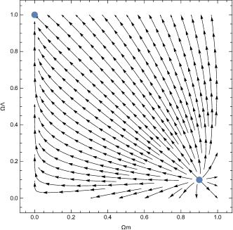
Figure 1: Phase space diagram for the dynamical system (20), (21). We consider $w_{m}=0$, for $n<1$. The unique attractor is the de Sitter point $A_{2}$.

Figure 2: Evolution diagrams with time, for various energy densities of the dynamical system (20), (21). We consider the initial conditions (a) $\Omega_{m}=0.4,$ $\Omega_{\Lambda}=0.1$ (b) $\Omega_{m}=0.7$, $\Omega_{\Lambda}=0.1$ (c) $\Omega_{m}=0.5$, $\Omega_{\Lambda}=0.2$ (d) $\Omega_{m}=0.2$, $\Omega_{\Lambda}=0.3$ (e) $\Omega_{m}=0.1$, $\Omega_{\Lambda}=0.9$ (f) $\Omega_{m}=0.2$, $\Omega_{\Lambda}=0.3$, for $n<1$ and $w_{m}=0$.

Table 1: Stationary points and physical parameters for the interaction model A.

Point	$\left(\mathbf{\Omega}_{m}\mathbf{,\Omega}_{\Lambda}\mathbf{,\Omega}_{z}\right)$	Existence	$\mathbf{w}_{tot}$	Acceleration
$A_{1}$	$\left(0,0,-1\right)$	Always	$-\frac{5}{6}$	Yes
$A_{2}$	$\left(0,1,0\right)$	Always	$-1$	Yes
$A_{3}$	$\left(1-\frac{n}{1+w_{m}},\frac{n}{1+w_{m}},0\right)$	$w_{m}\neq-1,(n=0,w_{m}>-1)\$or$~{}(n>0,w_{m}>-1+n)$	$w_{m}-n$	$w_{m}\leq n-\frac{1}{3}$

Table 2: Stationary points and stability conditions for the interaction model A.

Point	Eigenvalues	Stability
$A_{1}$	$\{\frac{1}{2},-\ \frac{5}{2}-3(w_{m}-n))\}$	Source
$A_{2}$	$\left\{-\frac{1}{2},-3(w_{m}-n+1)\right\}$	$w_{m}\geq n-1$
$A_{3}$	$\left\{3(w_{m}-n+1),3(w_{m}-n+\frac{5}{6})\right\}$	$w_{m}<n-1$

IV.3 Model B: $Q_{B}=9nH\rho_{\Lambda}$

For the second model of our analysis, where $Q_{B}=9nH\rho_{\Lambda}$, the field equations become

$$\frac{d\Omega_{\Lambda}}{d\ln a}=2\Omega_{\Lambda}\left[1+\frac{3}{4}(\Omega_{m}+\Omega_{\Lambda}\ -1)+\frac{1}{2}\Omega_{m}(1+3w_{m})-\Omega_{\Lambda}\right]-3n\Omega_{\Lambda},$$ (22)

$$\frac{d\Omega_{m}}{d\ln a}=2\Omega_{m}\left(1+\frac{3}{4}(\Omega_{m}+\Omega_{\Lambda}\ -1)+\frac{1}{2}\Omega_{m}(1+3w_{m})-\Omega_{\Lambda}\right)+3n\Omega_{\Lambda}-3\Omega_{m}(1+w_{m}),$$ (23)

The dynamical system (22), (23),admits three critical points with coordinates

$$B_{1}=\{0,0,-1\},~{}B_{2}=\{1,0,0\},B_{3}=\left\{\frac{n}{1+w_{m}},1-\frac{n}{1+w_{m}},0\right\}.$$

Point $B_{1}$ exists always and it corresponds to an empty universe with equation of state parameter $w_{tot}\left(B_{1}\right)=-\frac{5}{6}$, that is accelerating due to the contribution of the extra term introduced by the Finsler-Randers geometrical background. The eigenvalues of the linearized system are $\{\frac{(1-6n)}{2},-\ \frac{(5+6w_{m})}{2}\};$ hence the exact solution at the stationary point $B_{1}$ it is stable when $n>\frac{1}{6}~{}$and$~{}w_{m}>-\frac{5}{6}$. Thus this point is of great physical interest since it can describe a past or future acceleration phase.

Point $B_{2}~{}$describes a universe dominated by matter, $w_{tot}\left(B_{2}\right)=w_{m}$, and the exact solution at the point corresponds to an accelerated universe when $w_{m}<-\frac{1}{3}$. The eigenvalues of the linearized system are derived to be $\left\{3(w_{m}-n+1),\frac{(5+6w_{m})}{2}\right\},$ from where we observe that $B_{3}$ is an attractor when $n\leq\frac{1}{6}$& $w_{m}<n-1\$or$\ n>\frac{1}{6}~{}\&~{}w_{m}<-\frac{5}{6}$.

Point $B_{3}$ exists when $~{}w_{m}\neq-1,(1+w_{m})\geq n\geq 0\$and it has the same physical properties with point $A_{3}$. The eigenvalues of the linearized system near the stationary point are derived to be $\left\{\frac{(6n-1)}{2},-3(w_{m}-n+1)\right\}$, from where we infer that the exact solution at $B_{3}$ is stable for $n<\frac{1}{6}~{}\&~{}w_{m}>-1+n$.

The above results are summarized in Tables 3 and 4. In Figs. 3, 4 the evolution of trajectories for the dynamical system our study in phase space are presented.

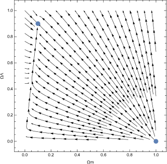
Figure 3: Phase space diagram for the dynamical system (22), (23). We consider $w_{m}=0$, for $n<1$. The unique attractor is the de Sitter point $B_{3}$.

Figure 4: Evolution diagrams with time, for various energy densities of the dynamical system (22), (23). We consider the initial conditions (a) $\Omega_{m}=0.4,$ $\Omega_{\Lambda}=0.1$ (b) $\Omega_{m}=0.7$, $\Omega_{\Lambda}=0.1$ (c) $\Omega_{m}=0.5$, $\Omega_{\Lambda}=0.2$ (d) $\Omega_{m}=0.2$, $\Omega_{\Lambda}=0.3$ (e) $\Omega_{m}=0.1$, $\Omega_{\Lambda}=0.9$ (f) $\Omega_{m}=0.2$, $\Omega_{\Lambda}=0.3$, for $n<1$ and $w_{m}=0$.

Table 3: Stationary points and physical parameters for the interaction model B.

Point	$\left(\mathbf{\Omega}_{m}\mathbf{,\Omega}_{\Lambda}\mathbf{,\Omega}_{z}\right)$	Existence	$\mathbf{w}_{tot}$	Acceleration
$B_{1}$	$\left(0,0,-1\right)$	Always	$-\frac{5}{6}$	Yes
$B_{2}$	$\left(1,0,0\right)$	Always	$w_{m}$	$w_{m}\leq-\frac{1}{3}$
$B_{3}$	$\left(\frac{n}{1+w_{m}},1-\frac{n}{1+w_{m}},0\right)$	$w_{m}\neq-1,(1+w_{m})\geq n\geq 0$	$-1+n$	$n\leq\frac{2}{3}$

Table 4: Stationary points and stability conditions for the interaction model B.

Point	Eigenvalues	Stability
$B_{1}$	$\{\frac{(1-6n)}{2},-\ \frac{(5+6w_{m})}{2}\}$	$n>\frac{1}{6}~{}\&~{}w_{m}>-\frac{5}{6}$
$B_{2}$	$\left\{3(w_{m}-n+1),\frac{(5+6w_{m})}{2}\right\}$	$n\leq\frac{1}{6}$& $w_{m}<n-1\$or$\ n>\frac{1}{6}~{}\&~{}w_{m}<-\frac{5}{6}$
$B_{3}$	$\{\frac{(6n-1)}{2},-3(w_{m}-n+1)\}$	$n<\frac{1}{6}~{}\&~{}w_{m}>-1+n$

IV.4 Model C: $Q_{C}=9nH(\rho_{\Lambda}+\rho_{m})$

For the third model of our analysis, where $Q_{C}=9nH(\rho_{\Lambda}+\rho_{m})$, the field equations read

$$\frac{d\Omega_{\Lambda}}{d\ln a}=2\Omega_{\Lambda}\left[1+\frac{3}{4}(\Omega_{m}+\Omega_{\Lambda}\ -1)+\frac{1}{2}\Omega_{m}(1+3w_{m})-\Omega_{\Lambda}\right]-3n\Omega_{\Lambda}-3n\Omega_{m},$$ (24)

$$\frac{d\Omega_{m}}{d\ln a}=2\Omega_{m}\left(1+\frac{3}{4}(\Omega_{m}+\Omega_{\Lambda}\ -1)+\frac{1}{2}\Omega_{m}(1+3w_{m})-\Omega_{\Lambda}\right)+3n\Omega_{\Lambda}+3n\Omega_{m}-3\Omega_{m}(1+w_{m}),$$ (25)

The latter dynamical system admits the following critical points

$$C_{1}=\{0,0,-1\},~{}C_{2\pm}=\{\frac{1}{2}\left(1\pm\sqrt{\frac{x}{(1+w_{m})}}\right),\frac{1}{2}\left(1\mp\sqrt{\frac{x}{(1+w_{m})}}\right),0\},$$

where we considered $x=1-4n+w_{m}.$

The universe described by the exact solution at the stationary point $C_{1}$ has the same physical quantities with those of points $A_{1}$ and $B_{1}$. The eigenvalues of the linearized system are

$$e_{1}\left(C_{1}\right) =-\frac{1}{2}\left(2+3w_{m}+3\sqrt{(1+w_{m})x}\right)~{}$$

$$e_{2}\left(C_{1}\right) =-\frac{1}{2}\left(2+3w_{m}-3\sqrt{(1+w_{m})x}\right)$$

from where we can infer that the point is an attractor when $\left\{\frac{1}{12}<n<\frac{1}{2},-\frac{2}{3}<w<-1+4n\right\}$, $\left\{n>\frac{1}{2},-\frac{2}{3},w<1\right\},~{}\left\{\frac{1}{12}<n<\frac{11}{72},-1+4n<w<\frac{5-36n}{36n-6}\right\},~{}\left\{\frac{11}{72}<n<\frac{1}{2},-1+4n<w<1\right\}.$

Point $C_{2\pm}~{}$exists for $\left\{n<0~{}\&~{}w_{m}\leq 4n-1\right\}\$or$\ \left\{n>0~{}\&~{}w_{m}\geqslant 4n-1\right\}$ and describes the same physical solutions with points $A_{3}$ and $B_{3}$. The equation of state parameter is $w_{m}\left(C_{2\pm}\right)=\frac{1}{2}\left(-1+w_{m}\pm\sqrt{\left(1+w_{m}\right)x}\right)$. From the linearized system around the critical points we determine the eigenvalues

$$e_{1}\left(C_{2\pm}\right) =\frac{1}{4}\left(2+3w_{m}\pm 9\sqrt{\left(1+w_{m}\right)x}\right)$$

$$+\frac{1}{4}\sqrt{13-36n\left(1+w_{m}\right)\mp 12\sqrt{\left(1+w_{m}\right)x}+6w_{m}\left(5+3w_{m}\mp 3\sqrt{\left(1+w_{m}\right)x}\right)},$$

$$e_{2}\left(C_{2\pm}\right) =\frac{1}{4}\left(2+3w_{m}\pm 9\sqrt{\left(1+w_{m}\right)x}\right)$$

$$-\frac{1}{4}\sqrt{13-36n\left(1+w_{m}\right)\mp 12\sqrt{\left(1+w_{m}\right)x}+6w_{m}\left(5+3w_{m}\mp 3\sqrt{\left(1+w_{m}\right)x}\right)}.$$

Therefore, point $C_{2-}$ is always unstable while point $C_{2+}$ is conditionally stable as shown in 6.

The above results are summarized in Tables 5,6 and 7. Moreover, in Figs. 5, 6 the evolution of trajectories for the dynamical system our study in phase space are presented.

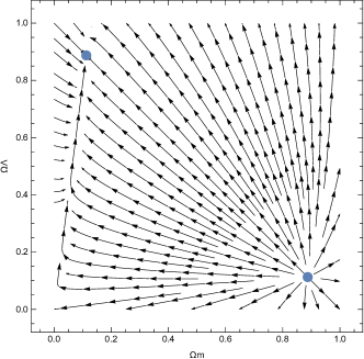
Figure 5: Phase space diagram for the dynamical system (24), (25). We consider $w_{m}=0$, for $n<1$. The unique attractor is point $C_{2}$.

Figure 6: Evolution diagrams with time, for the various densities for the dynamical system (24), (25). We consider the initial conditions (a) $\Omega_{m}=0.4,$ $\Omega_{\Lambda}=0.1$ (b) $\Omega_{m}=0.7$, $\Omega_{\Lambda}=0.1$ (c) $\Omega_{m}=0.5$, $\Omega_{\Lambda}=0.2$ (d) $\Omega_{m}=0.2$, $\Omega_{\Lambda}=0.3$ (e) $\Omega_{m}=0.1$, $\Omega_{\Lambda}=0.9$ (f) $\Omega_{m}=0.2$, $\Omega_{\Lambda}=0.3$, for $n<1$ and $w_{m}=0$.

Table 5: Stationary points and physical parameters for the interaction model C.

Point	$\left(\mathbf{\Omega}_{m}\mathbf{,\Omega}_{\Lambda}\mathbf{,\Omega}_{z}\right)$	Existence	$\mathbf{w}_{tot}$	Acceleration
$C_{1}$	$\left(0,0,-1\right)$	Always	$-\frac{5}{6}$	Yes
$C_{2\pm}$	$\left(\frac{1}{2}\left(1\pm\sqrt{\frac{x}{(1+w_{m})}}\right),\frac{1}{2}\left(1\mp\sqrt{\frac{x}{(1+w_{m})}}\right),0\right)$	$w_{m}\neq 0,n<0\ \&\ w_{m}\leq 4n-1$	$\frac{1}{2}\left(w_{m}-1\pm\sqrt{\left(1+w_{m}\right)x}\right)$	see 7
		$w_{m}\neq 0,n>0\ \&\ w_{m}\geqslant 4n-1$

Table 6: Stationary points and stability conditions for the interaction model C.

Point	Stability
$C_{1}$	$\left\{\frac{1}{12}<n<\frac{1}{2},-\frac{2}{3}<w<-1+4n\right\}$, $\left\{n>\frac{1}{2},-\frac{2}{3},w<1\right\}$
	$~{}\left\{\frac{1}{12}<n<\frac{11}{72},-1+4n<w<\frac{5-36n}{36n-6}\right\}$
	$\left\{\frac{11}{72}<n<\frac{1}{2},-1+4n<w<1\right\}$
$C_{2-}$	Unstable
$C_{2+}$	$n<0:~{}w_{m}<-1+4n,~{}-1<w_{m}<\frac{5-36n}{36n-6},~{}\frac{5-36n}{36n-6}<w_{m}<-\frac{2}{3}~{}$
	$0<n<\frac{1}{12}:w_{m}<-1,-1+4n<w_{m}<\frac{5-36n}{36n-6},\frac{5-36n}{36n-6}<w_{m}<-\frac{2}{3}~{}$
	$\frac{1}{12}<n<\frac{1}{6}:w_{m}<-1$
	$n>\frac{1}{6}:w_{m}<\frac{5-36n}{36n-6},\frac{5-36n}{36n-6}<w_{m}<-1$
	$n<\frac{1}{12}:w_{m}=\frac{5-36n}{36n-6}$
	$-\frac{2}{3}\leq w_{m}<1,~{}$ $n<\frac{6w_{m}+5}{36\left(1+w_{m}\right)}$.

Table 7: Acceleration conditions for the interaction model C for point $C_{2\textpm}$.

Point	Acceleration
$C_{2\pm}$	$n=0$
	$n>0$ & $w_{m}\leq-1$ or $n<\frac{1}{3}$ and $4n-1\leq w_{m}$
	$\frac{2}{3}>n\geqslant\frac{1}{3}$ and $w_{m}>\frac{4}{9n-6}-1$
	$n<0~{}$and $[4n-1\geqslant w_{m}~{}$or $w_{m}\geqslant-1]$

IV.5 Model D: $Q_{D}=$ $9nH^{3}\Omega_{z}$

In this scenario we shall consider an interaction of the form, $Q=Q\left(\Omega_{z}\right)$, that of course due to the constraint equation (16) means that

$$Q=Q\left(\Omega_{m},\Omega_{\Lambda}\right)$$

So, if we consider the interaction term to be $Q=$ $9nH^{3}\Omega_{z}$ then it follows

$$Q=9nH^{3}\left(\Omega_{m}+\Omega_{\Lambda}-1\right).$$

and our system is now

$$\frac{d\Omega_{\Lambda}}{d\ln a}=2\Omega_{\Lambda}\left[1+\frac{3}{4}(\Omega_{m}+\Omega_{\Lambda}\ -1)+\frac{1}{2}\Omega_{m}(1+3w_{m})-\Omega_{\Lambda}\right]-3n(\Omega_{m}+\Omega_{\Lambda}-1),$$ (26)

$$\frac{d\Omega_{m}}{d\ln a}=2\Omega_{m}\left[1+\frac{3}{4}(\Omega_{m}+\Omega_{\Lambda}\ -1)+\frac{1}{2}\Omega_{m}(1+3w_{m})-\Omega_{\Lambda}\right]+3n(\Omega_{m}+\Omega_{\Lambda}-1)-3\Omega_{m}(1+w_{m}),$$ (27)

The dynamical system (26), (27) admits three critical points with coordinates

$$D_{1}=\{0,1,0\},D_{2}=\{1,0,0\},D_{4}=\left\{6n\alpha,6n\alpha(5+6w_{m}),(5+6w_{m})\alpha\right\}$$

where$~{}\alpha=\left(36n(1+w_{m})-(5+6w_{m})\right)^{-1}.$ Point $D_{1}$ describes a de Sitter universe with equation of state parameter $w_{tot}\left(D_{1}\right)=-1$, where only the varying vacuum term contributes in the evolution of the universe. The eigenvalues are derived to be $\{-\frac{1}{2},-\ 3(1+w_{m})\},$ so for $w_{m}\geq-1$ the point is always an attractor and this point is of great physical interest.

Point $D_{2}~{}$describes a universe dominated by matter, $w_{tot}\left(D_{2}\right)=w_{m}$, and the exact solution at the point corresponds to an accelerated universe when $w_{m}\leq-\frac{1}{3}$. The eigenvalues of the linearized system are $\left\{3(1+w_{m}),\frac{(5+6w_{m})}{2}\right\},$ from where we observe that this point is an attractor only when $w_{m}<-1$.

Point $D_{3}$ exists when $~{}n<0,w_{m}>-\frac{5}{6}$ or $n>\frac{1}{6},0<w_{m}+\frac{5}{6}<n$ and it corresponds to a universe of two fluids and the contribution of the geometrical background of Finsler Randers that is always accelerating, that is, $w_{tot}\left(D_{3}\right)=-\frac{5}{6}$. Given that we consider the values of $n$ very small this solution describes a universe where matter decays in vacuum. The eigenvalues of the linearized system near the stationary point are $\left\{\frac{1}{2},-\frac{(5+6w_{m})}{2}\right\}$, so point $D_{3}$ is always a source, since one of the eigenvalues has always positive real part.

The above results are summarized in Tables 8 and 9. In Figs. 7, 8 the evolution of real trajectories for the dynamical system our study in phase space are presented.

Figure 7: Phase space diagram for the dynamical system (26), (27). We consider $\Omega_{m}=0,\;w_{m}=0$, for $n<1$. The unique attractor is the point $D_{1}$.

Figure 8: Evolution diagrams with time, for various energy densities of the dynamical system (26), (27). We consider the initial conditions (a) $\Omega_{m}=0.4,$ $\Omega_{\Lambda}=0.1$ (b) $\Omega_{m}=0.7$, $\Omega_{\Lambda}=0.1$ (c) $\Omega_{m}=0.5$, $\Omega_{\Lambda}=0.2$ (d) $\Omega_{m}=0.2$, $\Omega_{\Lambda}=0.3$ (e) $\Omega_{m}=0.1$, $\Omega_{\Lambda}=0.9$ (f) $\Omega_{m}=0.2$, $\Omega_{\Lambda}=0.3$, for $n<1$ and $w_{m}=0$.

Table 8: Stationary points and physical parameters for the interaction model D.

Point	$\left(\mathbf{\Omega}_{m}\mathbf{,\Omega}_{\Lambda}\mathbf{,\Omega}_{z}\right)$	Existence	$\mathbf{w}_{tot}$	Acceleration
$D_{1}$	$\left(0,1,0\right)$	Always	$-1$	Yes
$D_{2}$	$\left(1,0,0\right)$	Always	$w_{m}$	$w_{m}\leq-\frac{1}{3}$
$D_{3}$	$\left(6n\alpha,6n\alpha(5+6w_{m}),(5+6w_{m})\alpha\right)$	$n<0,w_{m}>-\frac{5}{6}$ or $n>\frac{1}{6},0<w_{m}+\frac{5}{6}<n$	$-\frac{5}{6}$	Yes

Table 9: Stationary points and stability conditions for the interaction model D.

Point	Eigenvalues	Stability
$D_{1}$	$\{-\frac{1}{2},-\ 3(1+w_{m})\}$	$w_{m}>-1$
$D_{2}$	$\left\{3(1+w_{m}),\frac{(5+6w_{m})}{2}\right\}$	$w_{m}<-1$
$D_{3}$	$\left\{\frac{1}{2},-\frac{(5+6w_{m})}{2}\right\}$	Source

IV.6 Model E: $Q_{E}=$ $9nH^{3}\Omega_{z}+9mH\rho_{m}$

Our system is now

$$\frac{d\Omega_{\Lambda}}{d\ln a}=2\Omega_{\Lambda}\left[1+\frac{3}{4}(\Omega_{m}+\Omega_{\Lambda}\ -1)+\frac{1}{2}\Omega_{m}(1+3w_{m})-\Omega_{\Lambda}\right]-3n(\Omega_{m}+\Omega_{\Lambda}-1)-3m\Omega_{m},$$ (28)

$$\frac{d\Omega_{m}}{d\ln a} =2\Omega_{m}\left[1+\frac{3}{4}(\Omega_{m}+\Omega_{\Lambda}\ -1)+\frac{1}{2}\Omega_{m}(1+3w_{m})-\Omega_{\Lambda}\right]$$ (29)

$$+3n(\Omega_{m}+\Omega_{\Lambda}-1)+3m\Omega_{m}-3\Omega_{m}(1+w_{m}),$$

The dynamical system (28), (29), admits three critical points with coordinates

$$E_{1}=\{0,1,0\},~{}E_{2}=\{1,0,0\},E_{3}=\{6nb,6nb(5+6w_{m}),(5+6w_{m}-6b)b\}.$$

where $b=\left(36n(1+w_{m})-(5+6w_{m})+6m\right)^{-1}.$ Point $E_{1}$ describes a de Sitter universe with equation of state parameter $w_{tot}\left(E_{1}\right)=-1$, where only the varying vacuum term contributes in the evolution of the universe. The eigenvalues are derived to be $\{-\frac{1}{2},-\ 3(1+w_{m}-m)\},$ so for $w_{m}>m-1$ the point is always an attractor and thus this solution is of great physical interest.

Point $E_{2}~{}$describes a universe dominated by the varying vacuum and matter; when $w_{m}=0$, point $E_{2}$ describes the $\Lambda$-CDM universe in the FR theory. The equation of state parameter is derived $w_{tot}\left(E_{2}\right)=w_{m}-m$, so this point describes an accelerated universe when $w_{m}\leq m-\frac{1}{3}$. The eigenvalues of the linearized system are $\left\{3(1+w_{m}-m),\frac{(5+6w_{m})-6m}{2}\right\}$ from where we can infer that the point is stable for $w_{m}<m-1.$Given though the existence condition $m-1\leq$ $w_{m}$ we consider the point to be unstable.

Point $E_{3}$ exists when $n,$ $m$ and $w_{m}$ are constrained as presented in Table 12. Similarly with point $D_{\mathbf{3}}$ this point corresponds to a universe of two fluids and the contribution of the geometrical background of Finsler Randers that is always accelerating$(w_{tot}\left(E_{3}\right)=-\frac{5}{6})$. The eigenvalues of the linearized system near the stationary point are $\left\{\frac{1}{2},-\frac{(5+6w_{m})}{2}+3m\right\}$, so point $E_{3}$ is always a source.

The above results are summarized in Tables 10 and 11. The trajectories of the dynamical system in the phase space are presented in Figs. 9, 10.

Figure 9: Phase space diagram for the dynamical system (28), (29). We consider $w_{m}=0$, for $n<1$. The unique attractor is point $E_{1}$.

Figure 10: Evolution diagrams with time, for various energy densities of the dynamical system (28), (29). We consider the initial conditions (a) $\Omega_{m}=0.4,$ $\Omega_{\Lambda}=0.1$ (b) $\Omega_{m}=0.7$, $\Omega_{\Lambda}=0.1$ (c) $\Omega_{m}=0.5$, $\Omega_{\Lambda}=0.2$ (d) $\Omega_{m}=0.2$, $\Omega_{\Lambda}=0.3$ (e) $\Omega_{m}=0.1$, $\Omega_{\Lambda}=0.9$ (f) $\Omega_{m}=0.2$, $\Omega_{\Lambda}=0.3$, for $n<1$ and $w_{m}=0$.

Table 10: Stationary points and physical parameters for the interaction model E.

Point	$\left(\mathbf{\Omega}_{m}\mathbf{,\Omega}_{\Lambda}\mathbf{,\Omega}_{z}\right)$	Existence	$\mathbf{w}_{tot}$	Acceleration
$E_{1}$	$\left(0,1,0\right)$	Always	$-1$	Yes
$E_{2}$	$\left(1-\frac{m}{1+w_{m}},\frac{m}{1+w_{m}},0\right)$	$w_{m}>-1,0\leq m\leq$ $1+w_{m}$	$w_{m}-m$	$w_{m}\leq m-\frac{1}{3}$
$E_{3}$	$\left(6nb,6nb(5+6w_{m}),(5+6w_{m}-6m)b\right)$	See Table 12	$-\frac{5}{6}$	Yes

Table 11: Stationary points and stability conditions for the interaction model E.

Point	Eigenvalues	Stability
$E_{1}$	$\{-\frac{1}{2},-\ 3(1+w_{m}-m)\}$	$w_{m}>m-1$
$E_{2}$	$\left\{3(1+w_{m}-m),\frac{(5+6w_{m})-6m}{2}\right\}$	$w_{m}<-1+m$
$E_{3}$	$\left\{\frac{1}{2},-\frac{(5+6w_{m})}{2}+3m\right\}$	Source

Table 12: Existence conditions for the stationary point $E_{4}$

Point	Existence	Existence
$E_{3}$	$m<0$	$n<0$ and $w_{m}\geq-\frac{5}{6}$
		$m+n=\frac{1}{6}$ and $5+6w_{m}=\frac{6m}{6n-1}$
		$n=0$ and $(w_{m}<m-\frac{5}{6}$  or $w_{m}>m-\frac{5}{6})$
		$m+n>\frac{1}{6}$and $6m+6n\geq 5+6w_{m}\geq\frac{6m}{6n-1}$
	$0<m\leq\frac{1}{6}$	$5+6w_{m}>0$ and [($n>0,m+n\leq\frac{1}{6},5+6w_{m}\leq\frac{6m}{6n-1}$) or ($m+n>\frac{1}{6},6m+6n\leq 5+6w_{m}$)]
	$m>\frac{1}{6}$	$m+n\leq\frac{1}{6}\$and $5+6w_{m}\geq\frac{6m}{6n-1}$
		$m+n\leq\frac{1}{6}$and $n<0,6m+6n\leq 5+6w_{m}$
		$n>0$ and $0<5+6w_{m}\leq 6m+6n$
	$m=0$, $5+6w_{m}>0$	$n<0~{}$or $[n\geq\frac{1}{6}~{}$and $n\geq\frac{5}{6}+w_{m}]$

IV.7 Model F: $Q_{F}=$ $9nH^{3}\Omega_{z}+9mH\rho_{\Lambda}$

Our system is now

$$\frac{d\Omega_{\Lambda}}{d\ln a}=2\Omega_{\Lambda}\left[1+\frac{3}{4}(\Omega_{m}+\Omega_{\Lambda}\ -1)+\frac{1}{2}\Omega_{m}(1+3w_{m})-\Omega_{\Lambda}\right]-3n(\Omega_{m}+\Omega_{\Lambda}-1)-3m\Omega_{\Lambda},$$ (30)

$$\frac{d\Omega_{m}}{d\ln a} =2\Omega_{m}\left[1+\frac{3}{4}(\Omega_{m}+\Omega_{\Lambda}\ -1)+\frac{1}{2}\Omega_{m}(1+3w_{m})-\Omega_{\Lambda}\right]$$ (31)

$$+3n(\Omega_{m}+\Omega_{\Lambda}-1)+3m\Omega_{\Lambda}-3\Omega_{m}(1+w_{m}),$$

The dynamical system (30), (31) admits three critical points with coordinates

$$F_{1}=\{0,1,0\},F_{2}=\{1,0,0\},F_{3}=\left\{6nc,6nc(5+6w_{m}),(5+6w_{m})(1-6m)c\right\},$$

where $c=\left(36n(1+w_{m})+(5+6w_{m})(6m-1)\right)^{-1}.$ Point $F_{1}~{}$describes a universe dominated by matter, $w_{tot}\left(F_{1}\right)=w_{m}$, and the exact solution at the point corresponds to an accelerated universe for $w_{m}\leq-\frac{1}{3}$. The eigenvalues of the linearized system are $\{\frac{(5+6w_{m})}{2},\ 3(1+w_{m}-m)\},$ from where we observe that this point is an attractor only when $w_{m}<-\frac{5}{6}\$and $1+w_{m}<m$. Thus this point provides a viable scenario of a matter dominated universe.

Point $F_{2}~{}$describes a universe dominated by the varying vacuum and matter; when $w_{m}=0$, point $F_{3}$ describes the $\Lambda$-CDM universe in the FR theory. The equation of state parameter is derived $w_{tot}\left(F_{2}\right)=m-1$, so this point describes an accelerated universe when $m\leq\frac{2}{3}$. The eigenvalues of the linearized system are $\left\{-3(1+w_{m}-m),3m-\frac{1}{2}\right\}$ from where we can infer that the point is stable for $m<\frac{1}{6}$ and $1+w_{m}>m.$We observe that for the theoretical values of m (very small) this is a stable point that describes an accelerated universe and thus it is extremely interesting from a physical point of view.

The existence conditions of point $F_{3}$ are given in Table 15. Similar with point $E_{\mathbf{3}},$ it corresponds to a universe of two fluids and the contribution of the geometrical background of Finsler Randers that is always accelerating$,~{}$that is, $w_{tot}\left(F_{3}\right)=-\frac{5}{6}$. The eigenvalues of the linearized system near the stationary point are $\left\{\frac{1}{2}-3m,-\frac{(5+6w_{m})}{2}\right\}$, so point $F_{3}$ is an attractor for $m>\frac{1}{6}~{}$and $w_{m}>-\frac{5}{6}$. The above results are summarized in Tables 13 and 14. In Figs. 11, 12 the evolution of trajectories for the dynamical system our study in phase space are presented.

Figure 11: Phase space diagram for the dynamical system (30), (31). We consider $w_{m}=0$, for $n<1$. The unique attractor is point $F_{3}$.

Figure 12: Evolution diagrams with time, for various energy densities of the dynamical system (30), (31). We consider the initial conditions (a) $\Omega_{m}=0.4,$ $\Omega_{\Lambda}=0.1$ (b) $\Omega_{m}=0.7$, $\Omega_{\Lambda}=0.1$ (c) $\Omega_{m}=0.5$, $\Omega_{\Lambda}=0.2$ (d) $\Omega_{m}=0.2$, $\Omega_{\Lambda}=0.3$ (e) $\Omega_{m}=0.1$, $\Omega_{\Lambda}=0.9$ (f) $\Omega_{m}=0.2$, $\Omega_{\Lambda}=0.3$, for $n<1$ and $w_{m}=0$.

Table 13: Stationary points and physical parameters for the interaction model F.

Point	$\left(\mathbf{\Omega}_{m}\mathbf{,\Omega}_{\Lambda}\mathbf{,\Omega}_{z}\right)$	Existence	$\mathbf{w}_{tot}$	Acceleration
$F_{1}$	$\left(1,0,0\right)$	Always	$w_{m}$	$w_{m}\leq-\frac{1}{3}$
$F_{2}$	$\left(\frac{m}{1+w_{m}},1-\frac{m}{1+w_{m}},0\right)$	$w_{m}>-1,0\leq m\leq$ $1+w_{m}$	$-1+m$	$m\leq\frac{2}{3}$
$F_{3}$	$\left(6nc,6nc(5+6w_{m}),(5+6w_{m})(6m-1)c\right)$	See Table 15	$-\frac{5}{6}$	Yes

Table 14: Stationary points and stability conditions for the interaction model F.

Point	Eigenvalues	Stability
$F_{1}$	$\{\frac{(5+6w_{m})}{2},\ 3(1+w_{m}-m)\}$	$w_{m}<-\frac{5}{6}\$and $1+w_{m}<m$
$F_{2}$	$\left\{-3(1+w_{m}-m),3m-\frac{1}{2}\right\}$	Attractor for$~{}m<\frac{1}{6}$ and $1+w_{m}>m$
$F_{3}$	$\left\{\frac{1}{2}-3m,-\frac{(5+6w_{m})}{2}\right\}$	Attractor for$~{}m>\frac{1}{6}~{}$and $w_{m}>-\frac{5}{6}$

Table 15: Existence conditions for the stationary point $F_{4}$

Point	Existence	Existence
$F_{3}$	$5+6w_{m}\geq 0$	$m=\frac{1}{6},n\neq 0$
		for $m<\frac{1}{6},~{}n<0$ or $m+n>\frac{1}{6}$
		for $m>\frac{1}{6},~{}n>0$ or $m+n<\frac{1}{6}$
	$5+6w_{m}\leq 0$	$n>0$ or $m+n<\frac{1}{6}$
		$n<0$ or $m+n>\frac{1}{6}$
	$m\neq\frac{1}{6}$	$m+n=\frac{1}{6}$ or $n=0$, $5+6w_{m}\neq 0$

IV.8 Model G: $Q_{G}=-3\left(1+\frac{3}{2}w_{m}\right)\Omega_{z}\Omega_{m}H^{3}$.

For the last model that we consider the term that is intrinsically by the FR model, namely $Q_{G}=-3\left(1+\frac{3}{2}w_{m}\right)\Omega_{z}\Omega_{m}H^{3}$, and the field equations are expressed as follows.

$$\frac{d\Omega_{\Lambda}}{d\ln a}=\ \frac{1}{2}[\Omega_{\Lambda}-\Omega_{\Lambda}^{2}+\Omega_{m}\ (2+3w_{m})(\Omega_{m}-1)+\Omega_{\Lambda}\Omega_{m}(7+9w_{m})]$$ (32)

$$\frac{d\Omega_{m}}{d\ln a}=-\frac{3}{2}\Omega_{m}(1+3w_{m})(1+\Omega_{\Lambda}-\Omega_{m})$$ (33)

The dynamical system (32),(33) admits four critical points with coordinates $\{\Omega_{m},\Omega_{\Lambda},\Omega_{z}\}$

$$G_{1}=\{0,0,-1\},~{}G_{2}=\{0,1,0\},~{}G_{3}=\{1,0,0\},~{}G_{4}=\{-\frac{1}{4+6w_{m}},-\frac{5+6w_{m}}{4+6w_{m}},-2-\frac{2}{4+6w_{m}}\}$$

Point $G_{1}$ always exists and describes an empty universe with equation of state parameter $w_{tot}\left(G_{1}\right)=-\frac{5}{6}.$ The universe accelerates with the contribution of the extra term introduced due to the Finsler-Randers Geometry. The eigenvalues of the linearized system near to point $G_{1}$ are $\{\frac{1}{2},-\frac{3}{2}(1+w_{m})\}$, and thus the point is always a source.

Point $G_{2}~{}$describes a de Sitter universe with equation of state parameter $w_{tot}\left(G_{2}\right)=-1$, where only the $\Lambda$ term contributes in the evolution of the universe. The eigenvalues are derived to be $\{-\frac{1}{2},-\frac{3}{2}(1+w_{m})\},$ from where we can infer that the point is an attractor when $w_{m}>-1$. Thus this point is of great physical interest.

Point $G_{3}$ always exists and describes a matter dominated universe that is accelerating for $w_{m}\leq-\frac{1}{3}.$The eigenvalues of the linearized system are $\{3(1+w_{m}),\frac{(5+6w_{m})}{2}\}$ and thus can be stable only for $w_{m}<-1.$

Point $G_{4}$ exists only for $w_{m}=-\frac{5}{6}$ in which case it again describes a matter dominated universe, but in this case it is always accelerating. By studying its eigenvalues for $w_{m}=-\frac{5}{6}$ though we deduce that the point is always unstable.

The above results are summarized in Tables 17 and 17. In addition in the Figs. 13,14 the evolution of trajectories for the dynamical system our study in phase space are presented.

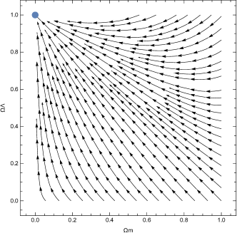
Figure 13: Phase space diagram for the dynamical system (32), (33). We consider $w_{m}=0$, for $n<1$. The unique attractor is the de Sitter point $G_{2}$.

Figure 14: Evolution diagrams with time, for various energy densities of the dynamical system (32), (33). We consider the initial conditions (a) $\Omega_{m}=0.4,$ $\Omega_{\Lambda}=0.1$ (b) $\Omega_{m}=0.7$, $\Omega_{\Lambda}=0.1$ (c) $\Omega_{m}=0.5$, $\Omega_{\Lambda}=0.2$ (d) $\Omega_{m}=0.2$, $\Omega_{\Lambda}=0.3$ (e) $\Omega_{m}=0.1$, $\Omega_{\Lambda}=0.9$ (f) $\Omega_{m}=0.2$, $\Omega_{\Lambda}=0.3$, for $n<1$ and $w_{m}=0$.

Table 16: Stationary points and physical parameters for the interaction model G.

Point	$\left(\mathbf{\Omega}_{m}\mathbf{,\Omega}_{\Lambda}\mathbf{,\Omega}_{z}\right)$	Existence	$\mathbf{w}_{tot}$	Acceleration
$G_{1}$	$\left(0,0,-1\right)$	Always	$-\frac{5}{6}$	Yes
$G_{2}$	$\left(0,1,0\right)$	Always	$-1$	Yes
$G_{3}$	$\left(1,0,0\right)$	Always	$w_{m}$	$w_{m}\leq-\frac{1}{3}$
$G_{4}$	$(-\frac{1}{4+6w_{m}},-\frac{5+6w_{m}}{4+6w_{m}},-2-\frac{2}{4+6w_{m}})$	$w_{m}=-\frac{5}{6}$	$-\frac{5}{6}$	Yes

Table 17: Stationary points and stability conditions for the interaction model G.

Point	Eigenvalues	Stability
$G_{1}$	$\{\frac{1}{2},-\frac{3}{2}(1+w_{m})\}$	Source
$G_{2}$	$\{-\frac{1}{2},-\frac{3}{2}(1+w_{m})\}$	$w_{m}>-1$
$G_{3}$	$\{3(1+w_{m}),\frac{(5+6w_{m})}{2}\}$	$w_{m}<-1$
$G_{4}$	$\{0,\frac{1}{2}\}$	Unstable

V Discussion

We performed, for the first time, a detailed study on the dynamics of the varying vacuum model in a Finsler-Randers geometrical background. Specifically in the homogeneous and isotropic spatially flat FLRW spacetime we assumed the existence of an ideal gas fluid source which couples with the varying vacuum terms. That scenario follows from the interacting models where interaction in the dark sector has been proposed as a possible scenario to explain the cosmological observations. For the gravitational theory, we consider that of Finsler Randers from where a new geometrodynamical term is introduced and affects the dynamical evolution.

The functional form of varying vacuum model is in generally unknown but a dominating quadratic term in the Hubble function has been found to be good a candidate. In this work we consider six different functional forms for the interaction between the components of the dark sector of the universe.

Models $Q_{A}$, $Q_{B}$ and $Q_{C}$ have been studied in a previous work in the case of GR VarVacGP . In this work we recover the results of the previous study, that is, the limit of GR relativity is recovered, while there exists one possible era in the cosmological history which corresponds to the epoch where only the geometrodynamical term of the FR geometry contributes.

In addition, we considered three new interaction models, namely $Q_{D}$, $Q_{E}$ and $Q_{F}$ which depend also on the geometrodynamical term of FR. For these three models the limit of GR is recovered while now there is a new cosmological solution where the geometrodynamical term contributes along the terms of the dark sector. These new epochs describe accelerated universe. As far as the stability of these exact solutions are concerned, they can be stable or unstable, depending on the coupling constants of the models.

Finally $Q_{G}$ is the case without varying vacuum term. In this scenario we found four critical points which describe the matter dominated era, the de Sitter universe, the vacuum space and an exact solution which correspond to a point where all the fluid source contributes in the cosmological evolution.

For model $Q_{A}$ there are three stationary points, point $A_{1}$ describes a universe dominated by the Finsler geometrodynamical terms and it is always a source, points $A_{2}$, $A_{3}$ describe the limit of GR, where $A_{2}$ describes the de Sitter universe and $A_{3}$ corresponds to the solution of GR where the matter source and the cosmological constant term contribute in the cosmological evolution. Notice that$A_{2}$ is an attractor when $w_{m}\geq n-1$ and $w_{m}$ is an attractor when $w_{m}<n-1$. In the case of a dust fluid, i.e. $w_{m}\,,$ the de Sitter universe is an attractor when $n\leq 1$. For model $Q_{B}$ we determined three stationary points: $B_{1}$ describes the Finsler epoch, while $B_{2}$ corresponds to the matter dominated era. Point $B_{3}$ has similar physical properties with point $A_{3}$, while de Sitter solutions are not provided by the model. In addition, the Finsler dominated epoch can be an attractor for specific values of the free parameters, as are the GR solutions of points $B_{2},$ $B_{3}$. Model $Q_{C}$ admits three stationary points, where $C_{1}$ describes the Finsler epoch and the two points $C_{\pm}$ describe the limit of GR which physical properties similar with that of point $A_{3}$.

Interaction models, $Q_{D}$, $Q_{E}$ and $Q_{F}$ provide three stationary points. Points $D_{1},~{}D_{2}$ are the limits of GR, which correspond to the matter dominated era and the de Sitter universe respectively. Point $D_{3}$ describes a universe where all the fluid components and the Finsler term contribute in the cosmological evolution.  Points $E_{1},$ $E_{2}$ have physical properties similar to those of points $A_{2},~{}A_{3}$ while the exact solution at point $E_{3}$ has similarities with the solutions at $D_{3}$. Furthermore, the dynamics close to points$F_{1},~{}F_{2}$is similar with that of $B_{2},~{}B_{3}$ and $F_{3}$ describes the same epoch with that of $D_{3}$.

As far as$Q_{G}$ model is concerned, the field equations admit four stationary points. Point $G_{1}$ describes an unstable exact solution where the cosmological fluid is described only by the Finsler terms. Point $G_{4}$ is always unstable and is has the same physical properties similar to that of $D_{3}$. Finally, points $G_{2},~{}G_{3}$ are the limit of GR, which correspond to the de Sitter and matter dominated eras, while one of two points is a unique attractor. Notice that for $w_{m}>-1$  the attractor is a de Sitter point.

From the results of this analysis we conclude that the varying vacuum cosmological scenario in the context of Finsler-Randers geometry can describe the basic epochs of cosmic history, however there are differences between the same phenomelogical interaction models in GR. In a future work we plan to test the performance of the current class of modified gravity models against the cosmological data.

- (1) A. G. Riess et al., Astron. J. 116, 1009 (1998)
- (2) S. Perlmutter et al., Astrophys. J. 517, 565 (1999)
- (3) N. Aghanim et al., arXiv:1807.06209 [astro-ph.CO]
- (4) E. J. Copeland, M. Sami and S. Tsujikawa, Int. J. Mod. Phys. D 15, 1753 (2006)
- (5) P. J. E. Peebles and B. Ratra, Rev. Mod. Phys. 75, 559 (2003)
- (6) T. Padmanabhan, Phys. Rept. 380, 235 (2003)
- (7) S. Weinberg, Rev. Mod. Phys. 61, 1 (1989)
- (8) T. P. Sotiriou and V. Faraoni, Rev. Mod. Phys. 82, 451 (2010)
- (9) A. De Felice and S. Tsujikawa, Living Rev. Rel. 13, 3 (2010)
- (10) T. Clifton, P. G. Ferreira, A. Padilla and C. Skordis, Phys. Rept. 513, 1 (2012)
- (11) S. Capozziello and M. De Laurentis, Phys. Rept. 509, 167 (2011)
- (12) S. Nojiri, S. D. Odintsov and V. K. Oikonomou, Phys. Rept. 692, 1 (2017)
- (13) Y. F. Cai, S. Capozziello, M. De Laurentis and E. N. Saridakis, Rept. Prog. Phys. 79, no. 10, 106901 (2016)
- (14) C. C. Perelman, Ann. Phys. 416, 168143 (2020)
- (15) E. Minas, E. N. Saridakis, P. Stavrinos and A. Triantafyllopoulos, Universe 5(3), 74 (2019)
- (16) G. W. Gibbons, C. A. R. Herdeiro, C. M. Warnick, M. C. Werner. Stationary Metrics and Optical Zermelo-Randers-Finsler Geometry. arXiv:0811.2877 (gr-qc) (2008)
- (17) S. Ikeda, E. N. Saridakis and P. C. Stavrinos. Phys. Rev. D 100 (2019)
- (18) A. Kouretsis, M. Stathakopoulos and P. C. Stavrinos. Phys. Rev. D, 79 (2009)
- (19) M. Hohmann, C. Pfeifer and N. Voicu. Phys. Rev. D 100 (2019)
- (20) Manuel Hohmann, Christian Pfeifer, Phys. Rev. D 95, 104021 (2017)
- (21) S. Vacaru, Int. J. Mod. Phy. D 21, 1250072 (2012)
- (22) E. Caponio and G. Stancarone, Int. J. Geom. Meth. Mod. Phys. Vol 13, No 4, (2016)
- (23) B. Edwards and A. Kostelecky. Phys. Lett. B, 786 (2018)
- (24) G. Randers, Phys. Rev. 59, 195 (1941)
- (25) P. Stavrinos, A. Kouretsis and M. Stathakopoulos, Gen. Rel. Grav. 40, 1403 (2008)
- (26) P. C. Stavrinos, Int. J. Theo. Phys. 44, 245 (2005)
- (27) H. Rund, The Differential Geometry of Finsler Spaces, Springer (1955)
- (28) J. D. Bekenstein, Phys. Rev. D 48, 3641 (1993)
- (29) R. Miron and M. Anastasiei, ‘The geometry of Lagrange spaces:Theory and Applications’, Kluwer Academic.Dordrecht (1994)
- (30) D. Bao, S. S. Chern and Z. Shen, ‘An Introduction to Riemann-Finsler Geometry’, Springer, New York (2000)
- (31) S. Vacaru, P. Stavrinos, E. Gaburov, D. Gontsa, Clifford and Riemann - Finsler Structures in Geometric Mechanics and Gravity. Balkan Press (2005), arXiv: gr-qc/0508023
- (32) P. Stavrinos, F. Diakogiannis, Grav. Cosmol. 10, 269 (2004)
- (33) G. S. Asanov, Finsler Geometry, Relativity and Gauge Theories, Kluwer Academic Publishers Group, Holland (1985)
- (34) A. Triantafyllopoulos, P.C Stavrinos. Classical and Quantum Gravity. Vol.35, Is.8, (2018)
- (35) P. C. Stavrinos, M. Alexiou, Raychaudhuri equation in the Finsler Randers spacetime and Generalized scalar tensor theories . Int. Jour. Geom. Meth. Mod. Phys. 15 (03), 1850039, (2018)
- (36) S. Basilakos, P.Stavrinos. ”Cosmological equivalence between the Finsler-Randers space-time and DGP gravity model”. Phys. Rev. D, Vol 87, Is. 4 (2013).
- (37) S. Basilakos, A. Kouretsis, E. Saridakis, P. C. Stavrinos. Phys. Rev. D, D 88, Is. 12 (2013). arXiv: 1311.5915 [grqc]. ”Resembling dark energy and modified gravity with Finsler - Randers Cosmology.
- (38) P. Stavrinos. Weak Gravitational field in Finsler-Randers Space and Raychchaudhuri Equation. General Relativity and Gravitation Vol.44, No12, pp.3029. (2012).
- (39) G. Silva, R.V. Maluf, C.A.S. Almeida. A nonlinear dynamics for the scalar field in Randers spacetime. Phys. Let. B V. 766, (2017), P. 263-267
- (40) T. Singh, R. Chaubey and Ashutosh Singh. ”Bounce conditions for FRW models in modified gravity theories”. Eur.Phys. Jour. Plus volume 130, Article number: 31 (2015)
- (41) Rakesh Raushan R. Chaubey ”Finsler Randers cosmology in the framework of a particle creation mechanism: a dynamical systems perspective”. Eur. Phys.Jour.Plus V. 135, 228 (2020)
- (42) R. Chaubey, B. Tiwari, Anjani Kumar Shukla and Manoj Kumar. Finsler Randers Cosmological Models in Modified Gravity Theories Proceedings of the National Academy of Sciences, India Section A: Physical Sciences V. 89, pages757-768 (2019).
- (43) I. L. Shapiro and J. Solá, JHEP 0202 (2002) 006; Phys.Lett. B 475 (2000) 236; J. Solá, J. Phys. A 41 (2008) 164066; I. L. Shapiro and J. Solá, Phys. Lett. B 682, 105 (2009); S. Basilakos, MNRAS 395, 2347 (2009); Astron. Astrphys., 508, 575 (2009); S. Basilakos, M. Plionis and Solá, Phys. Rev. D80 (2009) 083511; J. Grande, J. Solá, S. Basilakos and M. Plionis, JCAP 08, 007 (2011); S. Basilakos, J. A. S. Lima and J. Solá, MNRAS 431, 923 (2013); E. L. D. Perico, J. A. S. Lima, S. Basilakos and J. Solá, Phys. Rev. D 88, 063531 (2013); J. Solá and and A. Gómez-Valent, Int. J. Mod. Phys. D 24, 1541003 (2015); A. Gómez-Valent, J. Solá and S. Basilakos, JCAP 01, 004 (2015); V. K. Oinonomou, S. Pan and R. C. Nunes, Int. J. Mod. Phys. A 32, 1750129 (2017); S. Pan, Mod. Phys. Lett. A 33, 1850003 (2018); J. Solá, J. de Cruz Pérez and A. Gómez-Valent, EPL 121, 39001 (2018); S. Basilakos, N. Mavromatos and J. Solá, JCAP 12, 025 (2019); Phys. Rev. D 101, 045001 (2020); Phys. Lett. B. 803, 135342 (2020)J. A. S.
- (44) Lima, F. E. Silva and R. C. Santos, Class. Quant. Grav.25, 205006 2008
- (45) G. Steigman, R. C. Santos and J. A. S. Lima, JCAP, 06, 033 2009
- (46) Lima, J. A. S.; Basilakos, S.; Costa, F. E. M., Phys. Rev D.,86, 103534 2012
- (47) J. A. S. Lima, M. O. Calvao, I. Waga, “Cosmology, Thermodynamics and Matter Creation, Frontier Physics, Essays in Honor of Jayme Tiomno, World Scientific, Singapore (1990), [arXiv:0708.3397];
- (48) I. Prigogine et al., Gen. Rel. Grav.21, 767 1989
- (49) M. O. Calvao, J. A. S. Lima and I. Waga, Phys. Lett. A162, 223-226 1992
- (50) J. A. S. Lima and A. S. M. Germano, Phys. Lett. A 170, 373 1992
- (51) W. Zimdahl and D. Pavon, Gen. Relativ. Grav.,12, 1259 1994
- (52) W. Zimdahl, J. Triginer and D. Pavon Phys. Rev. D.,54, 6101 1996
- (53) J. A. S. Lima, S. Basilakos, F. E. M. Costa, Phys.Rev. D. 86 103534
- (54) L. Parker, Phys. Rev. Lett. 21, 562 (1968)
- (55) L. Parker, Phys. Rev. 183, 1057 (1969)
- (56) L. Parker, Phys. Rev. D3, 346 (1970)
- (57) L. H. Ford and L. Parker, Phys. Rev. D16, 245 (1977)
- (58) Ya. B. Zeldovich and A. A. Starobinsky, JETP Lett. 34 1159 (1972)
- (59) a. B. Zeldovich and A. A. Starobinsky, JETP Lett. 26, 252 (1977)
- (60) A. A. Grib, B. A. Levitskii and V. M. Mostepanenko, Theor. Math. Phys. 19, 59 (1974)
- (61) A. A. Grib, B. A. Levitskii and V. M. Mostepanenko, Gen. Rel. Grav. 7, 535 (1976)
- (62) A. A. Grib, B. A. Levitskii and V. M. Mostepanenko, Vacuum Quantum Effects in Strong Fields, Friedman Laboratory Publishing, Saint Petersburg, Russia (1994)
- (63) E. Schrödinger, Physica 6, 899 (1939)
- (64) G. Steigman, R. C. Santos and J. A. S. Lima, JCAP 06, 033 (2009)
- (65) J. A. S. Lima, J. F. Jesus and F. A. Oliveira, JCAP 11, 027 (2010)
- (66) J. A. S. Lima, L. L. Graef, D. Pavon and S. Basilakos, JCAP 10, 042 (2014)
- (67) R. C. Nunes and D. PavĂłn, Phys. Rev. D 91, 063526 (2015)
- (68) C. Pigozzo, S. Carneiro, J. S. Alcaniz, H. A. Borges and J. C. Fabris, JCAP 05, 022 (2016)
- (69) L. Amendola, Phys. Rev. D 62, 043511 (2000)
- (70) L. Amendola and C. Quercellini, Phys. Rev. D 68, 023514 (2003)
- (71) R. G. Cai and A. Wang, JCAP 0503, 002 (2005)
- (72) D. Pavón and W. Zimdahl, Phys. Lett. B 628, 206 (2005)
- (73) S. del Campo, R. Herrera and D. Pavón, Phys. Rev. D 78, 021302 (2008)
- (74) S. del Campo, R. Herrera and D. Pavón, JCAP 0901, 020 (2009)
- (75) C. Wetterich, Astron. Astrophys. 301, 321 (1995)
- (76) J. D. Barrow and T. Clifton, Phys. Rev. D 73, 103520 (2006)
- (77) L. Amendola, G. Camargo Campos and R. Rosenfeld, Phys. Rev. D 75, 083506 (2007)
- (78) D. Pavón and B. Wang, Gen. Rel. Grav. 41, 1 (2009)
- (79) L. P. Chimento, Phys. Rev. D 81, 043525 (2010)
- (80) F. Arevalo, A. P. R. Bacalhau and W. Zimdahl, Class. Quant. Grav. 29, 235001 (2012)
- (81) W. Yang, S. Pan, R. Herrera and S. Chakraborty, Phys. Rev. D 98, no.4, 043517 (2018)
- (82) A. Paliathanasis, S. Pan and W. Yang, Int. J. Mod. Phys. D 28, 1950161 (2019)
- (83) P. Tsiapi and S. Basilakos, MNRAS 485 (2019)
- (84) W. Yang, N. Banerjee, A. Paliathanasis and S. Pan, Phys. Dark Univ. 26, 100383 (2019)
- (85) S. Pan, J. de Haro, W. Yang and J. Amorós, [arXiv:2001.09885 [gr-qc]]
- (86) V. Salvatelli, N. Said, M. Bruni, A. Melchiorri and D. Wands, Phys. Rev. Lett. 113, 181301 (2014)
- (87) R. Murgia, S. Gariazzo and N. Fornengo, JCAP 1604 (2016)
- (88) R. C. Nunes, S. Pan and E. N. Saridakis, Phys. Rev. D 94, no.2, 023508 (2016)
- (89) S. Pan and G. Sharov, MNRAS 472, no.4, 4736 (2017)
- (90) G. S. Sharov, S. Bhattacharya, S. Pan, R. C. Nunes and S. Chakraborty, MNRAS 466, no.3, 3497 (2017)
- (91) W. Yang, N. Banerjee and S. Pan, Phys. Rev. D 95, no.12, 123527 (2017)
- (92) W. Yang, S. Pan and D. F. Mota, Phys. Rev. D 96, no.12, 123508 (2017)
- (93) W. Yang, S. Pan and J. D. Barrow, Phys. Rev. D 97, no.4, 043529 (2018)
- (94) S. Pan, A. Mukherjee and N. Banerjee, MNRAS 477, no.1, 1189 (2018)
- (95) W. Yang, S. Pan, E. Di Valentino, R. C. Nunes, S. Vagnozzi and D. F. Mota, JCAP 09, 019 (2018)
- (96) D. Begue, C. Stahl and S.-S. Xue, Nucl. Phys. B 940, 312 (2019)
- (97) M. Szydlowski, T. Stachowiak and R. Wojtak, Phys. Rev. D 73, 063516 (2006)
- (98) W. Yang, S. Pan and A. Paliathanasis, MNRAS 482, 1007 (2019)
- (99) S. Pan, W. Yang, C. Singha and E. N. Saridakis, Phys. Rev. D 100, no.8, 083539 (2019)
- (100) S. Pan, W. Yang, E. Di Valentino, E. N. Saridakis and S. Chakraborty, Phys. Rev. D 100, no.10, 103520 (2019)
- (101) S. Pan, W. Yang and A. Paliathanasis, MNRAS 493, 3114 (2020)
- (102) W. Yang, S. Pan, R. C. Nunes and D. F. Mota, JCAP 04, 008 (2020)
- (103) E. Di Valentino, A. Melchiorri, O. Mena and S. Vagnozzi, [arXiv:1908.04281 [astro-ph.CO]]
- (104) E. Di Valentino, A. Melchiorri, O. Mena and S. Vagnozzi, Phys. Rev. D 101, no.6, 063502 (2020)
- (105) S. Pan, G. S. Sharov and W. Yang, [arXiv:2001.03120 [astro-ph.CO]]
- (106) I. Prigogine, J. Geheniau, E. Gunzig, P. Nardone, Gen. Rel. Grav. 21, 767 (1989)
- (107) L. R. W. Abramo and J. A. S. Lima, Class. Quant. Grav. 13, 2953 (1996)
- (108) E. Gunzig, R. Maartens and A. V. Nesteruk, Class. Quant. Grav. 15, 923 (1998)
- (109) W. Zimdahl, Phys. Rev. D 61, 083511 (2000)
- (110) R. C. Nunes, Int. J. Mod. Phys. D 25, 1650067 (2016)
- (111) J. de Haro and S. Pan, Class. Quant. Grav. 33, no.16, 165007 (2016)
- (112) S. Pan, J. Haro, A. Paliathanasis and R. J. Slagter, MNRAS 460, 1445 (2016)
- (113) R. C. Nunes and S. Pan, MNRAS 459, no.1, 673 (2016)
- (114) A. Paliathanasis, J. D. Barrow and S. Pan, Phys. Rev. D 95, 103516 (2017)
- (115) G. Papagiannopoulos, P. Tsiapi, S. Basilakos and A. Paliathanasis, Eur. Phys. J. C 80, 55 (2020)
- (116) G. Papagiannopoulos, S. Basilakos, A Paliathanasis and P. C. Stavrinos, Class. Quant. Grav. 34, 22 (2017)
- (117) E. J. Copeland, A. R. Liddle and D. Wands, Phys. Rev. D. 57, 4686 (1998)
- (118) C. R. Fadragas and G. Leon, Class. Quant. Grav. 31, 195011 (2014)
- (119) S. Wiggins, Introduction to applied nonlinear dynamical systems and chaos, Springer-Verlag, New York, (1990)
- (120) A. Paliathanasis, G. Papagiannopoulos, S. Basilakos and J. D. Barrow, Eur. Phys. J. C 79, 723 (2019)
- (121) S. Basilakos, G. Leon, G. Papagiannopoulos and E. N. Saridakis, Phys. Rev. D 100, 043524 (2019)
- (122) G. Papagiannopoulos, J. D. Barrow, S. Basilakos, A. Giacomini and A. Paliathanasis, Phys. Rev. D 95, 024021 (2017)
- (123) G. Leon and E. N. Saridakis, JCAP 1504, 031 (2015)
- (124) G. Leon, Int. J. Mod. Phys. E 20, 19 (2011)
- (125) T. Gonzales, G. Leon and I. Quiros, Class. Quant. Grav. 23, 3165 (2006)
- (126) A. Giacomini, S. Jamal, G. Leon, A. Paliathanasis and J. Saveedra, Phys. Rev. D 95, 124060 (2017)
- (127) G. Chee and Y. Guo, Class. Quantum Grav. 29, 235022 (2012) [Corrigendum: Class. Quant. Grav. 33, 209501 (2016)]
- (128) S. Mishra and S. Chakraborty, Eur. Phys. J. C 79, 328 (2019)
- (129) H. Farajollahi and A. Salehi, JCAP 07, 036 (2011)
- (130) A. Paliathanasis, Phys. Rev. D 101, 064008 (2020)
- (131) G. Panotopoulos, A. Rincon, N. Videla and G. Otalora, Eur. Phys. J. C 80, 286 (2020)
- (132) M. Kerachian, G. Acquaviva, G.L. Gerakopoulos, Phys. Rev. D 101, 043535 (2020)