Efficient and Effective Query Auto-Completion

Abstract.

Query Auto-Completion (QAC) is an ubiquitous feature of modern textual search systems, suggesting possible ways of completing the query being typed by the user. Efficiency is crucial to make the system have a real-time responsiveness when operating in the million-scale search space. Prior work has extensively advocated the use of a trie data structure for fast prefix-search operations in compact space. However, searching by prefix has little discovery power in that only completions that are prefixed by the query are returned. This may impact negatively the effectiveness of the QAC system, with a consequent monetary loss for real applications like Web Search Engines and eCommerce.

In this work we describe the implementation that empowers a new QAC system at eBay, and discuss its efficiency/effectiveness in relation to other approaches at the state-of-the-art. The solution is based on the combination of an inverted index with succinct data structures, a much less explored direction in the literature. This system is replacing the previous implementation based on Apache SOLR that was not always able to meet the required service-level-agreement.

1. Introduction

The Query Auto-Completion (QAC) problem we consider can be formulated as follows. Given a collection $\mathcal{S}$ of scored strings and a partially-completed user query $Q$, find the top-$k$ scored completions that match $Q$ in $\mathcal{S}$. For our purposes, a completion is a full (i.e., completed) query for which the search engine, that indexes a large document collection, returns a relevant and non-empty recall set. The collection $\mathcal{S}$ is usually a query log consisting in several million user queries seen in the past, with scores taken as a function of the frequencies of the queries. The straightforward approach of suggesting the “most popular queries” (Bar-Yossef and Kraus, 2011) (i.e., the ones appearing more often) works well for real-world applications like eBay search.

At eBay, the QAC system helps users to formulate queries to explore 1.4 billion live listings better (e.g., with less spell errors) and faster (as we also include relevant category constraints). This is important for desktop users but, in particular, for the growing number of users of mobile devices. In fact, as QAC is expected to happen instantaneously, these systems have a low-millisecond service-level-agreement (SLA). The previous system implemented at eBay, based on Apache SOLR, was not always able to meet the SLA and had a sub-optimal memory footprint. This motivated the development of eBay’s new QAC system.

In this paper, we share the basic building blocks of the retrieval part of the system. In short, it is based on a combination of succinct data structures, an inverted index, and tailored retrieval algorithms. We also provide an open-source implementation in C++ of the presented techniques – available at https://github.com/jermp/autocomplete – with a reproducible experimental setup that includes state-of-the-art baselines.

Lastly, we remark that a production version of this system was implemented in eBay’s Cassini search framework and can serve about 135,000 query per seconds at 50% CPU utilization on a 80-core machine. (The 99-quantile latency is below 2 milliseconds and the average latency is about 190 $\mu$s.)

2. Related work

The QAC problem has been studied rather extensively since its popularization by Google around 2004. The interested reader can refer to the general surveys by Cai et al. (2016) and Krishnan et al. (2017) for an introduction to the problem.

Following the taxonomy given by Krishnan et al. (2017), we have two major auto-completion query modes – prefix-search and multi-term prefix-search – that have been implemented and are in wide-spread use. Our own implementation at eBay is no exception, thus these are the query modes we also focus on.

Informally speaking, searching by prefix means returning strings from $\mathcal{S}$ that are prefixed by the concatenation of the terms of $Q$; a multi-term prefix-search identifies completions where all the terms of $Q$ appear as prefixes of some of the terms of the completions, regardless their order. We will describe and compare these two query modes in details in Section 3. Prefix-search is supported efficiently by representing $\mathcal{S}$ with a trie (Fredkin, 1960) and many papers discuss this approach (Hsu and Ottaviano, 2013; Bar-Yossef and Kraus, 2011; Mitra and Craswell, 2015; Mitra et al., 2014; Shokouhi and Radinsky, 2012; Shokouhi, 2013). Multi-term prefix-search is, instead, accomplished via an inverted index built from the completions in $\mathcal{S}$ (Bast and Weber, 2006; Ji et al., 2009). In particular, if we assign integer identifiers (docids) to the completions, an inverted list is materialized for each term that appears in $\mathcal{S}$ and stores the identifiers of the completions that contain the term. (As we are going to illustrate in the subsequent sections, how docids are assigned to the completions is fundamental for the efficiency of the inverted index and, hence, of the overall QAC system.)

For example, if $Q$ is “shrimp dip rec”, then a plausible completion found by prefix-search could be “shrimp dip recipes”. A multi-term prefix-search could return, instead, “shrimp bienville dip recipe” or “recipe for appetizer shrimp chipolte dip”. Note that all terms of $Q$ are prefixed by some terms of these two example completions but in no specific order.

The focus of this paper is on the query modes, rather than on the ranking of results. As already stated, we consider the popular strategy of ranking the results by their frequency within a query log. There have been some studies comparing different ranking mechanism for a single query mode, e.g., prefix-search (Di Santo et al., 2015). However, little attention was given to the efficiency/effectiveness trade-off between different query modes, with an exception in this regard being the experimentation by Krishnan et al. (2017). They also report significant variations in effectiveness by varying query mode.

We now briefly summarize two results that are closely related to the contents of this paper because both use an inverted index. Bast and Weber (2006) merge the inverted lists into blocks and store their unions to reduce the number of lists. As we will see, this is crucial to sensibly boost the responsiveness of the QAC system in the case of single-term queries. For queries involving several terms, Ji et al. (2009) propose an efficient algorithm to quickly check whether a completion belongs to the union of a set $L$ of inverted lists. Instead of trivially computing the union, the idea is to check whether the terms in the completion overlap with those corresponding to the inverted lists in $L$.

Other Approaches. Although inherently different from the direction we pursue here, other approaches may include sub-string search, where each term of $Q$ can occur as a sub-string of a completion. However, to the best of our knowledge, there are no implementations of this query mode but only a discussion by Chaudhuri and Kaushik (2009). Also, suggesting $n$-grams from the indexed documents was found to be very effective in absence of a query log (Bhatia et al., 2011).

1 Complete(query, $k$) :

2       prefix, suffix $=$ Parse(dictionary, query)

3       if prefix was not found : return [ ]

4       $[\ell,r]$ $=$ dictionary.LocatePrefix(suffix)

5       if $[\ell,r]$ is invalid : return [ ]

6       $[p,q]$ $=$ completions.LocatePrefix(prefix, $[\ell,r]$)

7       if $[p,q]$ is invalid : return [ ]

8       topk_ids $=$ RMQ($[p,q]$, $k$)

9       strings $=$ ExtractStrings(topk_ids)

10       return strings

11      

12

(a)

1 Complete(query, $k$) :

2       prefix, suffix $=$ Parse(dictionary, query)

3       $[\ell,r]$ $=$ dictionary.LocatePrefix(suffix)

4       if $[\ell,r]$ is invalid : return [ ]

5       topk_ids $=$ ConjunctiveSearch(prefix, $[\ell,r]$, $k$)

6       strings $=$ ExtractStrings(topk_ids)

7       return strings

8      

9

(b)

Figure 1. Auto-Completion algorithms based on prefix-search (a) and conjunctive-search (b).

3. Efficient and Effective Query Auto-Completion

Here we describe the QAC algorithm used at eBay – in essence, based on the multi-term prefix-search query mode that we are going to call conjunctive-search from now on.

We begin with an overview of the different steps involved in the identification of the top-$k$ completions for a query in Section 3.1. The aim of such section is to introduce the data structures and algorithms involved in the search. From Section 1, recall that we use $\mathcal{S}$ to denote the set of scored strings from which completions are returned. As we will see next, we have several data structures built from $\mathcal{S}$, such as: (1) a dictionary, storing all its distinct terms; (2) a representation of the completions that allows efficient prefix-search; (3) an inverted-index. Section 3.2 discusses the implementation details of these data structures. Lastly, in Section 3.3 we explain how to implement conjunctive-search efficiently.

3.1. Query Processing Steps

In this section we detail the processing steps that are executed to identify the top-$k$ completions for a query. We are going to illustrate the pseudo code given in Fig. 1 that shows two different solutions to the QAC problem, respectively based on prefix-search (a) and conjunctive-search (b).

A detail of crucial importance for the search efficiency is that we do not manipulate scores directly, rather we assign docids to completions in decreasing-score order. (Ties broken lexicographically.) This implies that if a completion has a smaller docid than another, it has a “better” score as well. As we are going to illustrate next, this docid-assignment strategy substantially simplifies the implementation of both prefix-search and conjunctive-search.

With this initial remark in mind, we now consider an example of $\mathcal{S}$ in Table 1a. Suppose $k=3$. If the query $Q$ is “bm”, then the algorithm in Fig. 1a based on prefix-search would return the completions having docid 1, 2, and 4. (The other implementation in Fig. 1b would return the same results.) Now, if $Q$ is “sport”, the algorithm in Fig. 1b would find 2, 4, and 6, as the top-3 docids. (Note that the algorithm in Fig. 1a is not able to answer this query.)

Parsing. We consider the query as composed by a set of terms, each term being a group of characters separated by white spaces. The query can possibly end without a white space: in this case the last query term is considered to be incomplete. The first processing step involves parsing the query, i.e., dividing it into two separate parts: a prefix and a suffix. The suffix is just the last term (possible, incomplete). The prefix is made up of all the terms preceding the suffix: each of them, say $t$, is looked up in a dictionary data structure by means of the operation called $\textup{{Locate}}(t)$ that returns the lexicographic integer id of $t$. For example, the id of the term “sedan” is 7, in the example in Fig. 1b. (If term $t$ does not belong to the dictionary then an invalid id is returned to signal this event.)

Table 1. An example set of completions seen as strings and integer sets in (a). The integer sets are obtained by replacing the terms with their ids as given by the dictionary in (b).

docids	completions	sets
9	audi	$\langle 2\rangle$
6	audi a3 sport	$\langle 2,1,8\rangle$
3	audi q8 sedan	$\langle 2,6,8\rangle$
8	bmw	$\langle 3\rangle$
5	bmw x1	$\langle 3,10\rangle$
1	bmw i3 sedan	$\langle 3,4,7\rangle$
4	bmw i3 sport	$\langle 3,4,8\rangle$
2	bmw i3 sportback	$\langle 3,4,9\rangle$
7	bmw i8 sport	$\langle 3,5,8\rangle$

(a)

termids	terms	inverted lists
1	a3	$\langle 6\rangle$
2	audi	$\langle 3,6,9\rangle$
3	bmw	$\langle 1,2,4,5,7,8\rangle$
4	i3	$\langle 1,2,4\rangle$
5	i8	$\langle 7\rangle$
6	q8	$\langle 3\rangle$
7	sedan	$\langle 1,3\rangle$
8	sport	$\langle 4,6,7\rangle$
9	sportback	$\langle 2\rangle$
10	x1	$\langle 5\rangle$

(b)

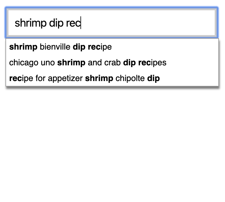
(a) conjunctive-search

(b) prefix-search

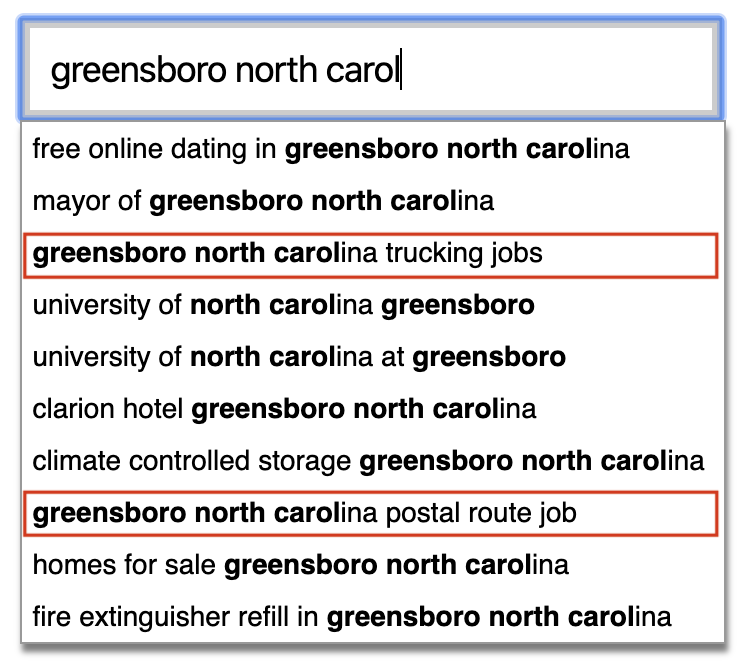
(c) conjunctive-search

Figure 2. Some example of searches on the AOL query log. In (a), a simple prefix-search returns no results at all, whereas conjunctive-search does. In (b) and (c) we see that both search modes return a full set of results (top-10), that are significantly different: only the results enclosed within the boxes are in common. The example shows that the first two results returned by conjunctive-search have a better score than the first result of prefix-search; the 4th, 5th, 6th, and 7th results of conjunctive-search have all better score than the second result of prefix-search.

Prefix-search. Let us assume for the moment that all terms in the prefix are found in the dictionary. Let $PS$ indicate the concatenation of prefix and suffix. The Complete algorithm in Fig. 1a, based on prefix-search, returns the top-$k$ completions from $\mathcal{S}$ that are prefixed by $PS$ and comprises two steps. First, the dictionary is used to obtain the lexicographic range $[\ell,r]$ of all the terms that are prefixed by the suffix, using the operation $\textup{{LocatePrefix}}(\mbox{\emph{suffix}})$. If there is no string in the dictionary that is prefixed by suffix, then the range $[\ell,r]$ is invalid and the algorithm returns no results.

Otherwise, the operation $\textup{{LocatePrefix}}(\mbox{\emph{prefix}},[\ell,r])$ is executed on a data structure representing the completions of $\mathcal{S}$. More precisely, this data structure does not represent the completions as strings of characters, but as (multi-) sets of integers, each integer begin the lexicographic id of a dictionary term. Refer to Table 1a for a pictorial example. In Fig. 1a, we indicate such data structure with the name completions. The operation $\textup{{LocatePrefix}}(\mbox{\emph{prefix}},[\ell,r])$ returns, instead, the lexicographic range $[p,q]$ of the completions in $\mathcal{S}$ that are prefixed by $PS$. Again, if there are no strings in completions that are prefixed by $PS$, then prefix-search fails.

Let us consider a concrete example for the query “bmw i3 s”, with $\mathcal{S}$ as in Table 1a. Then $\mbox{\emph{prefix}}=\langle 3,4\rangle$ and suffix $=$ “s”. The first operation $\textup{{LocatePrefix}}($“s”$)$ on the dictionary of Table 1b returns $[7,9]$. The second operation $\textup{{LocatePrefix}}(\langle 3,4\rangle,[7,9])$, instead, returns the range $[6,8]$.

We then proceed with the identification of the top-$k$ completions. This step retrieves the smallest docids of the completions whose lexicographic id is in $[p,q]$. If we materialize the list of the docids following the lexicographic order of the completions (such as the column “docids” in Table 1a) – say docids – then identifying the top-$k$ docids boils down to support range-minimum queries (RMQ) (Muthukrishnan, 2002) over $\mbox{\emph{docids}}[p,q]$. Note that this is possible because of the used docid-assignment. We recall that $\textsf{{RMQ}}(p,q)$ returns the position of the minimum element in $\mbox{\emph{docids}}[p,q]$. Specifically, we have that $\mbox{\emph{docids}}[i]=x$, where $x$ is the docid of the $i$-th lexicographically smallest completion. In other words, docids is a map from the lexicographic id of a completion to its docid. The column “docids” in Table 1a shows an example of such sequence. Continuing the same example as before for the query “bmw i3 s”, we have got the range $[6,8]$, thus we have to report the $k$ smallest ids in $\mbox{\emph{docids}}[6,8]$. For example, if $k=1$, then $\textsf{{RMQ}}(6,8)=6$ and we return $\mbox{\emph{docids}}[6]=1$.

Conjunctive-search. A conjunctive-search is a multi-term prefix-search that uses an inverted index. At a high-level point of view, what we would like to do is to identify completions containing all the terms specified in the prefix and any term that is prefixed by the suffix. We can do this efficiently by computing the intersection between the inverted lists of the term ids in the prefix and the union of the inverted lists of all the terms in $[\ell,r]$. In Section 3.3 we will describe efficient implementations of this algorithm.

For our example query “bmw i3 s”, the intersection between the inverted lists in Table 1b of the terms “bmw” and “i3” gives the list $X=[1,2,4]$. Since the range $[\ell,r]$ is $[7,9]$ in our example, the union of the inverted lists 7, 8, and 9 is $Y=[1,2,3,4,6,7]$. We then return the docids in $X\cap Y$, i.e., $[1,2,4]$. In fact, it is easy to verify that such completions of id 1, 2, and 4, are the ones having all the two terms of the prefix and any term among the ones prefixed by “s”, that are “sedan”, “sport” and “sportback”.

Again, observe that since the lists are sorted by docids and we assigned docids in decreasing score order, the best results are those appearing before as we process the lists from left to right.

We claim that conjunctive-search is more powerful than prefix-search, for the following reasons.

• It is not restricted to just the completions that are prefixed by $PS$. In fact, what if we have a query like “i3” or “bmw sport i8”? The simple prefix-search is not able to answer. (No completion is prefixed by “i3” or “bmw sport”.)

• There could exist a completion that is not prefixed by $PS$ but has a better score than that of some results identified by prefix-search. Consider the practical examples in Fig. 2. over the AOL dataset, one of the publicly available datasets we use in our experimental analysis.

• It can also be issued when a query term is out of the vocabulary. In that case, prefix-search is not able to answer at all (unless the term is the suffix), whereas conjunctive-search can use the other query terms in the prefix.

However, as we will experimentally show in Section 4, this effectiveness does not come for free in terms of efficiency.

Reporting. After the identification of the set of (at most) $k$ top ids, that we indicate with topk_ids in Fig. 1, the last step reports the final identified completions, i.e., those strings having ids in topk_ids. What we need is a data structure supporting the operation $\textup{{Access}}(x)$ that returns the string in $\mathcal{S}$ having lexicographic id $x$. Once we have a completion, that is a (multi-) set of term ids, we can use the dictionary to Extract each term from its id, hence reconstructing the actual completion’s string.

3.2. Data Structures

In the light of the query processing steps described in Section 3.1 and their operational requirements, we now discuss the implementation details of the data structures they use.

The Dictionary. The string dictionary data structure has to support Locate, LocatePrefix and Extract. An elegant way of representing in compact space a set of strings while supporting all the three operations, is that of using Front Coding compression (FC) (Martínez-Prieto et al., 2016). FC provides good compression ratios when the strings share long common prefixes and remarkably fast decoding speed.

We use a (standard) two-level data structure to represent the dictionary. We chose a block size $B$ and compress with FC the $\lceil|\mbox{\emph{dictionary}}|/(B+1)\rceil$ buckets, with each bucket comprising $B$ compressed strings (except, possibly, the last). The first strings of every bucket are stored uncompressed in a separate header stream. It follows that both operations Locate and LocatePrefix are supported by binary searching the header strings and then scanning: one single bucket for Locate; or at most two buckets for LocatePrefix. The operation Extract is even faster than Locate because only one bucket has to be scanned without any prior binary search. Clearly the bucket size $B$ controls a space/time trade-off (Martínez-Prieto et al., 2016): larger values of $B$ favours space effectiveness (less space overhead for the header), whereas smaller values favours query processing speed. In Section 4 we will fix the value of $B$ yielding a good space/time trade-off.

The Completions. For representing the completions in $\mathcal{S}$, we need a data structure supporting LocatePrefix which returns the lexicographic range of a given input string. (In the following discussion, we assume $\mathcal{S}$ to be sorted lexicographically.)

As already mentioned in Section 2, a classic option is the trie (Fredkin, 1960) data structure, that is a labelled tree with root-to-leaf paths representing the strings of $\mathcal{S}$. In our setting, we need an integer trie and we adopt the data structure described by Pibiri and Venturini (2017, 2019a), augmented to keep track of the lexicographic range of every node. More specifically, a node $n$ stores the lexicographic range spanned by its rooted subtrie: if $\alpha$ is the string spelled-out by the path from the root to $n$ and $[p,q]$ is the range, then all the strings prefixed by $\alpha$ span the contiguous range $\mathcal{S}[p,q]$. It follows that, for a trie level consisting in $m$ nodes, the sequence formed by the juxtaposition of the ranges $[p_{1},q_{1}]\ldots[p_{m},q_{m}]$ is sorted by the ranges’ left extremes, i.e., $p_{i}<p_{i+1}$ for $i=1,\ldots,m-1$. Therefore, to allow effective compression is convenient to represent such sequence as two sorted integer sequences: the sequence $L$ formed by the left extremes, such that $L[i]=p_{i}-i$; and the sequence obtained by considering the range sizes and taking its prefix sums. Each level of the trie is, therefore, represented by 4 sorted integer sequences: nodes, pointers, left extremes, and range sizes. Another option to represent $\mathcal{S}$ is to use FC compression as similarly done for the dictionary data structure. We now discuss advantages and disadvantages of both options, and defer the experimental comparison to Section 4.

• Tries achieve compact storage because common prefixes between the strings are represented once by a shared root-to-node path in the tree. Prefix coding is clearly better than that of FC but the trie needs more redundancy for the encoding of the tree topology and range information.

• Although prefix searches in the trie are supported in time linear in the size of the searched pattern (assuming $O(1)$ time spent per level), the traversal process is cache-inefficient for long patterns. The binary search needed to locate the front-coded buckets is not cache-friendly as well (and includes string comparisons), but is compensated by the fast decoding of FC.

• Another point of comparison is that of supporting the $\textup{{Access}}(i)$ operation that returns the $i$-th smallest completion from $\mathcal{S}$. This is needed to implement the last step of processing, that is to report the identified top-$k$ completions as strings. The trie data structure can not support Access without explicit node-to-parent relationships, whereas FC offers a simple solution taking, again, time proportional to $B$. If we opt to use a trie, a simple way of supporting Access is to explicitly represent the completions in a forward index that is, essentially, a map from the docid to the completion. (The use of a forward index is also crucial for the efficient implementation of conjunctive-search we will describe in Section 3.3.)

In conclusion, we have two different and efficient ways of supporting prefix-search and Reporting: either a trie plus a forward index, or FC compression.

Range-Minimum Queries. The identification of the top-$k$ docids in a given lexicographic range follows a standard approach (Muthukrishnan, 2002; Hsu and Ottaviano, 2013). The algorithm iteratively finds the $k$ smallest elements in $\mbox{\emph{docids}}[p,q]$. To do so, we maintain a min-heap of ranges, each of these keeping track of the position of the minimum element in the range. At each step of the loop: (1) we pop from the heap the interval having the minimum element; (2) add it to the result set; (3) push onto the heap the two sub-ranges respectively to the left and to the right on the minimum element. Correctness is immediate. To answer a range-minimum query we build and store the cartesian tree of the array docids. It is well-known that such tree can be represented in just $2n+o(n)$ bits, with $n$ being the size of the array, using a succinct encoding such as balanced parentheses (BP) (Fischer and Heun, 2011). Since the time complexity of a RMQ is $O(1)$ and the heap contains $O(k)$ elements (at each iteration, we push at most two ranges but always remove one) it follows that this algorithm has a worst-case complexity of $\Theta(k\log k)$.

The Inverted Index. Inverted indexes are subject of deep study and a wealth of different techniques can be used to represent them in compressed space (Pibiri and Venturini, 2019c), while allowing efficient query processing. What we need is an algorithm for supporting list intersections: details on how this can be achieved by means of the Next Greater-than or Equal-to (NextGeq) primitive are discussed by many papers (Moffat and Zobel, 1996; Pibiri and Venturini, 2019c; Ottaviano and Venturini, 2014; Pibiri, 2019). The operation $\textup{{NextGeq}}_{t}(x)$ returns the element $z\geq x$ from the inverted list of the term $t$ if such element exists, otherwise the sentinel $\infty$ (larger than any possible value) is returned.

3.3. Multi-term Prefix-search Query Mode: Conjunctive-search

In this section we discuss efficient implementations of the conjunctive-search algorithm introduced in Section 3.1. We begin our discussion by describing a simple approach that uses just an inverted index; then highlight its main efficiency issues and present solutions to solve them. Remember that the objective of this query mode is to return completions that contain all the terms in the prefix and any term that is prefixed by the suffix.

Using an Inverted Index. A first approach is illustrated in Fig. 3. The idea is to iterate over the elements of the intersection (lines 7-8) between the inverted lists of the prefix and, for each element, check whether it appears in any of the inverted lists of the terms in $[\ell,r]$ (inner loop in lines 9-18). Directly iterating over the elements of the intersection, rather than computing the whole intersection between the inverted lists, saves time when the intersection has many results because we only need the first, i.e., smallest, $k$ results. (Remember that we assign docids in decreasing score order.)

To implement the check for a given docid x, we maintain a heap of list iterators: one iterator for each inverted list. To be clear, an iterator over a list is an object that has the capability of skipping over the list values using the NextGeq primitive, and advancing to the element coming next the one currently “pointed to”. At each step of the inner loop, the heap selects the iterator that currently “points to” the minimum docid. If such docid is smaller than x, then we can advance the iterator to the successor of x by calling NextGeq and re-heapify the heap (line 13). Otherwise we have that such docid is larger-than or equal-to x. If it is equal to x, then a result is found. Then in any case we can break the loop because either a result was found, or the docid is strictly larger then x, thus also every other element in the heap is larger than x. Fig. 4 details a step-by-step example showing the behavior of the algorithm.

1 ConjunctiveSearch(prefix, $[\ell,r]$, $k$) :

2       intersection $=$ index.IntersectionIterator(prefix)

3       results $=$ [ ], heap $=$ [ ]

4       for $i=\ell$; $i\leq r$; $i=i+1$ :  

5             heap.Append(index.Iterator($i$))

6            

7      heap.MakeHeap()

8      

9      while intersection.HasNext() and !heap.Empty() :  

10             x $=$ intersection.Next()

11            

12            while !heap.Empty() :  

13                  

14                  top $=$ heap.Top()

15                  

16                  if top.docid $>$ x : break

17                  

18                  if top.docid $<$ x :  

19                        

20                        if top.NextGeq(x) $<$ $\infty$ : heap.Heapify()

21                         else : heap.Pop()

22                        

23                  else :

24                        

25                        results.Append(x)

26                         if |results| $==$ $k$ : return results

27                         break

28                        

29                  

30            

31      

32      return results

33

Figure 3. Heap-based conjunctive-search algorithm.

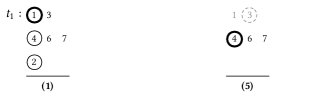
Figure 4. The steps performed by the algorithm in Fig. 3 for the query “bmw i3 s”. We check the elements in the intersection between the inverted lists of “bmw” and “i3”, that are $[1,2,4]$, over the lists for the terms “sedan” ($t_{1}:1,3$), “sport” ($t_{2}:4,6,7$) and “sportback” ($t_{3}:2$). The elements pointed to by the iterators in the heap are the ones circled with solid lines. At the beginning we are checking docid 1 and, since heap’s top element is 1, that is the first result. At the second step we are now checking docid 2. Since the heap still returns 1, we advance the iterator to $\textup{{NextGeq}}_{t_{1}}(2)=3$. At step 3, the heap returns the element 2 that is another found result. At step 4 we are now checking docid 4, thus we advance the iterator by calling $\textup{{NextGeq}}_{t_{3}}(4)$. Since the inverted list of term $t_{3}$ has no element larger-than or equal to $4$, then $\textup{{NextGeq}}_{t_{3}}(4)$ will be equal to the sentinel $\infty$ and the iterator over such list is popped-out from the heap. The same happens for the iterator of the list $t_{1}$ at step 5. The algorithm finally finds the last result 4, at step 6.

Let $m=r-\ell+1$ be the size of the range $[\ell,r]$. The filling and making of the heap (lines 4-6) takes $O(m)$ time. For every element of the intersection, we execute the inner loop (lines 9-18) that has a worst-case complexity of $t_{\emph{\text{check}}}=O(m\log m\times t_{\textup{{NextGeq}}})$. Therefore, the overall complexity is $O(m+t_{\emph{\text{intersection}}}+|\mbox{\emph{intersection}}|\times t_{\emph{\text{check}}})$. We point out that this theoretical complexity is, however, excessively pessimistic because $t_{\emph{\text{check}}}$ may be very distant from its worst-case scenario, and indeed be even $O(1)$ when the body of the else branch at line 15 is executed (lines 16-18). Also, the heap cost of $O(m\log m)$ progressively vanishes as iterators are popped out from the data structure (line 14). In fact, as we will better show in Section 4, the algorithm is pretty fast unless $m$ is very large. Handling large values of $m$ efficiently is indeed the problem we address in the following.

Lastly, we point out that the approach by Bast and Weber (2006) can be implemented on top of this algorithm. The crucial difference is that their algorithm makes use of a blocked inverted index, with inverted lists grouped into blocks and merged. We will compare against their approach in Section 4.

Forward Search. The approach coded in Fig. 3 is clearly more convenient than explicitly computing the union of all the inverted lists in $[\ell,r]$ and then searching it for every single docid belonging to the intersection. However, it is inefficient when the range $[\ell,r]$ is very large. We remark that this case is actually possible and very frequent indeed, because it represents the case where the user has typed just few characters of the suffix and, potentially, a large number of strings are prefixed by such characters. We now discuss how to solve this problem efficiently.

The idea, illustrated in Fig. 5, is to avoid accessing the inverted lists of the terms in the range $[\ell,r]$ (and, thus, avoid using a heap data structure as well) but rather check whether the terms of a completion intersects the ones in $[\ell,r]$. More precisely, for every completion in the intersection we check if there is at least one term $t$ of the completion such that $t\geq\ell$ and $t\leq r$. Given that completions do not contain many terms (see also Table 2), a simple scan of the completion suffices to implement the check as fast as possible. While this is not constant-time from a theoretical point of view, in practice it is. This idea of falling back to a forward search was introduced by Ji, Li, Li, and Feng (2009).

Take again the example query “bmw i3 s”. We check whether the completions of docid 1, 2, and 4, seen as integer sets, intersect the range $[7,9]$. By looking at Table 1a, it is easy to see that the last term id of such completions is always in $[7,9]$.

The complexity of the algorithm is then essentially dependent from the size of the intersection and the time needed to Extract a completion, that is $O(t_{\emph{\text{intersection}}}+|\mbox{\emph{intersection}}|\times t_{\textup{{Extract}}})$. Compared to the heap-based algorithm in Fig. 3, we are improving the time for checking a given docid (and saving a factor of $O(m)$), by relying of the efficiency of the Extract operation. We clearly expect $t_{\textup{{Extract}}}$ to be more efficient than the worst-case complexity of $t_{\emph{\text{check}}}$ that is $O(m\log m\times t_{\textup{{NextGeq}}})$, especially for large values of $m$. Note that although the worst-case theoretical complexity is independent from $m$, in practice the size of $m$ influences the probability that the test in line 6 succeeds: the larger is $m$, the higher the probability and the faster the running time of the algorithm.

However, the behavior of the heap-based algorithm for small values of $m$ is not intuitive and its running time could not necessarily be worse than having to issue many Extract operations (when, for example, the test in line 11 succeeds frequently). Again, the experimental analysis in Section 4 will compare the two different approaches. Instead, it should be intuitive why this algorithm produces the same results as the heap-based one: they are just the “inverted version” of each other, i.e., one is using an inverted index whereas the other is using a “forward” approach. Therefore, correctness is immediate.

To Extract a completion given its id (line 6), we can either use a forward index or FC compression, as we have discussed in Section 3.2. Using the latter method means to actually decode a completion, a process involving scanning and memory-copy operations, whereas the former technique provides immediate access to the completion, that is $t_{\textup{{Extract}}}=O(1)$, at the expense of storing an additional data structure (the forward index). Therefore, we have a potential space/time trade-off here, that we investigate in Section 4.

1 ConjunctiveSearch(prefix, $[\ell,r]$, $k$) :

2       results $=$ [ ]

3       intersection $=$ index.IntersectionIterator(prefix)

4       while intersection.HasNext() :  

5             x $=$ intersection.Next()

6             completion = Extract(x)

7             if completion intersects $[\ell,r]$ :  

8                   results.Append(x)

9                   if |results| $==$ $k$ : break

10            

11      return results

12

Figure 5. Forward conjunctive-search algorithm.

Single-Term Queries. Now we highlight another efficiency issue: the case for single-term queries. We recall and remark that such queries are always executed when users are typing, hence they are the most frequent case. This motivates the need for having a specific algorithm for their resolution.

Single-term queries represent a special case in that the prefix is empty (we only have the suffix). This means that there is no intersection over which to iterate, rather every single docid from 1 to $|\mathcal{S}|$ would have to be considered by both algorithms coded in Fig. 3 and 5. This makes them very inefficient on such queries. In this case, the “classic” approach of finding the $k$ smallest elements from the inverted lists in the range $[\ell,r]$ with a heap is more efficient than checking every docid (using a similar approach to that coded in Fig. 3). However, it is still slow on large ranges because an iterator for every inverted list in the range $[\ell,r]$ has to be instantiated and pushed onto the heap.

We can elegantly solve this problem with another RMQ data structure. Let us consider the list minimal, where $\mbox{\emph{minimal}}[i]$ is the first docid of the $i$-th inverted list. (In other words, minimal is the “first column” of the inverted index.) If we build a RMQ data structure on such list, $\textup{{RMQ}}(\ell,r)$ identifies the inverted list from which the minimum docid is returned. Therefore, we instantiate an iterator on such list and push onto the heap its next docid along with the left and right sub-ranges. We proceed recursively as explained in the previous section. (Now, if the element at the top of the heap comes from an iterator we do not push left and right sub-ranges.) The key difference with respect to the “classic” heap-based algorithm mentioned above, is that an iterator is instantiated over an inverted list if and only if an element has to be returned from it.

For the example in Table 1b, the minimal list will be $[$6, 3, 1, 1, 7, 3, 1, 4, 2, 5$]$ and, if the single-term query is “s”, then we ask for RMQ over $\mbox{\emph{minimal}}[7,9]$. Assume $k=3$. The first returned docid is therefore 1, the first for the inverted list of the term “sedan”. We pushed onto the heap the next id from such list, 3, as well as the right sub-range $[8,9]$. The element at the top of the heap is now 2, the first for the inverted list of the term “sportback”. There are no more docids from such list, thus we remove the sub-range $[8,9]$ and add the sub-range $[8,8]$. We finally return the id 3, again from the list of the term “sedan”. Observe that the iterator on the inverted list of the term id 8 (“sport”, in this case) is never instantiated.

4. Experiments

In this section we report on the experiments we conducted to assess the efficiency and the effectiveness of the described QAC algorithms. The experiments are organized as follows. We first benchmark and tune the data structures used by the algorithms in Section 4.1. With the tuning done, we then compare the efficiency of various options to perform conjunctive-search, also with respect to the efficiency of prefix-search, in Section 4.2. We then discuss effectiveness and memory footprint of the various solutions in Section 4.3 and 4.4 respectively.

Table 2. Dataset statistics.

Statistic	AOL	MSN	EBAY
Queries	$10,142,395$	$7,083,363$	$7,295,104$
Uncompressed size in MiB	299	208	189
Unique query terms	$3,825,848$	$2,590,937$	$323,180$
Avg. num. of chars per term	14.58	14.18	7.32
Avg. num. of queries per term	7.87	8.15	73.02
Avg. num. of terms per query	2.99	2.99	3.24

Datasets. We used three large real-world query logs in English: AOL (Pass et al., 2006) and MSN (Inc., 2006) (both available at https://jeffhuang.com/search_query_logs.html), and EBAY that is a proprietary collection of queries collected during the year 2019 from the US .com site. We do not apply any text processing to the logs, such as capitalization, but index the strings as given in order to ensure accurate reproducibility of our results. For AOL and MSN, the score of a query is the number of times the query appears in the log (i.e., its frequency count) (Hsu and Ottaviano, 2013); for EBAY, the score is assigned by some machine learning facility that is irrelevant for the scope of this paper. As already mentioned, integer ids (docids) have been assigned to queries in decreasing score order. Ties are broken lexicographically. Table 2 summarizes the statistics.

Experimental Setting. Experiments were performed on a server machine equipped with Intel i9-9900K cores (@3.60 GHz), 64 GB of RAM DDR3 (@2.66 GHz) and running Linux 5 (64 bits).

For researchers interested in replicating the results on public datasets, we provide the C++ implementation at https://github.com/jermp/autocomplete. We used that implementation to obtain the results discussed in the paper. The code was compiled with gcc 9.2.1 with all optimizations enabled, that is with flags -O3 and -march=native.

The data structures were flushed to disk after construction and loaded in memory to be queried. The reported timings are average values among 5 runs of the same experiment. All experiments run on a single CPU core. We use $k=10$ for all experiments.

4.1. Tuning the Data Structures

For the experiments in this section, we used the (larger) AOL dataset given that consistent results were also obtained for MSN and EBAY.

The Dictionary. As explained in Section 3.2, we represent the dictionary using a 2-level data structure compressed with Front Coding (FC). We are interested in benchmarking the time for three operations, namely Extract, Locate, and LocatePrefix, by varying the bucket size that directly controls the achievable space/time trade-off. The result of the benchmark is reported in Table 3. The timings, expressed in $\mu$sec per string, are recorded by executing 100,000 queries and computing the average. Such queries are strings belonging to the dictionary and shuffled at random to avoid locality of access. To benchmark the operation LocatePrefix, we retain 0%, 25%, 50% and 75% of the characters of a given input string (the case for 100% would correspond to a Locate operation; in the case of 0%, we always retain 1 single character instead of 0). As we can see from the results reported in the table, the space decreases but the time increases for increasing values of bucket size. The Extract operation is roughly $4\times$ faster than Locate. The timings for LocatePrefix are pretty much the same for all percentages except 0%: in that case strings comparisons are much faster, resulting in a better execution time. For all the following experiments, we choose a bucket size of 16 that yields a good space/time trade-off: Extract takes 0.1 $\mu$sec on average, with Locate and LocatePrefix around half of a microsecond and, compared to the size of the uncompressed file which is 56.85 MiB, FC offers a compression ratio of approximately $1.69\times$. (On MSN and EBAY, the compression ratio are $1.67\times$ and $1.61\times$ respectively.)

Table 3. Front-coded dictionary benchmark on the AOL dataset, by varying bucket size. Timings are in $\mu$sec per string. The size of the uncompressed file is 56.85 MiB, that is an average of 15.58 bytes per string (bps).

Bucket	MiB	bps	Extract	Locate	LocatePrefix
size					0%	25%	50%	75%
4	40.95	11.22	0.12	0.46	0.15	0.67	0.76	0.66
8	36.35	9.96	0.11	0.43	0.17	0.62	0.65	0.58
16	33.64	9.22	0.10	0.41	0.18	0.61	0.62	0.57
32	32.16	8.81	0.12	0.44	0.22	0.69	0.69	0.65
64	31.39	8.60	0.16	0.54	0.57	0.89	0.92	0.89
128	30.99	8.49	0.24	0.74	0.51	1.21	1.31	1.30
256	30.79	8.44	0.42	1.20	0.96	2.07	2.23	2.24

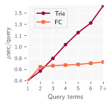
(a) LocatePrefix

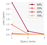
(b) RMQ

Figure 6. Timings for (a) LocatePrefix and (b) RMQ in $\mu$sec per string on AOL. Results for FC are relative to a bucket size of 16 strings.

The Completions. We now compare the two distinct approaches of representing the completions with a trie or Front Coding. Regarding the trie, we recall from Section 3.2 that it is represented by four sorted integer sequences. We follow the design recommended in (Pibiri and Venturini, 2019a, 2017) of using Elias-Fano to represent nodes and pointers for its fast, namely constant-time, random access algorithm and powerful search capabilities. For the same reasons, we also adopt Elias-Fano to compress the left extremes and range sizes. With Elias-Fano compression, the trie takes a total of 88.80 MiB that is 9.18 bytes per completions (bpc). Most of the space is spent, not surprisingly, in the encoding of the nodes: 6.57 bpc (71.6%). Pointers take 0.84 bpc (9.17%), left extremes take 1.08 bpc (11.73%) and range sizes take 0.69 bpc (7.5%). The completions compressed with FC, using a bucket size of 16, take 97.98 MiB, i.e., 10.13 bpc. Thus the trie takes 9.4% less space than FC.

To record the time for the LocatePrefix operation, we partitioned the completions by the number of terms $d$, for $d$ from 1 to 6. All completions having $d\geq 7$ terms (7+) are placed in the same partition. From each partition, we then sample 100,000 queries at random. We firs observed that the time is pretty much independent from the size of the suffix because the average number of characters per term is very low. (Basically, 14 for both AOL and MSN, and 7 for EBAY. See Table 2.) Therefore, the only influence comes from the number of query terms and we show the result in Fig. 6a.

While the Trie query time constantly increases by $\approx$200 nanoseconds per level (basically, 2 cache misses per level), the query time for FC is almost insensitive to the size of the query. Therefore as expected, the Trie is beaten by FC as query length increases due to cache-misses. As a net result, better cache efficiency paired with fast decoding makes FC roughly $2\times$ faster than the Trie for queries having more than 4 terms.

Range-Minimum Queries. The timings for RMQ are reported in Fig. 6b. As it is intuitive, the timing strongly depends on the size of the range. Such size is exponentially decreasing when both the number of terms and the percentage of characters retained from the suffix increases. As a matter of fact, the RMQ time is practically negligible from 3 terms onwards.

Table 4. Inverted index compression benchmark on AOL in average bits per integer (bpi).

Method	BIC	DINT	PEF	EF	OptVB	VB	Simple16
bpi	14.14	15.08	15.10	17.15	17.33	20.95	21.74

Inverted Index Compression. For the QAC problem, the inverted lists are very short on average because the completions themselves comprise only few terms (see Table 2). Therefore, we cannot expect a great deal of compression effectiveness as, for example, the one for Web pages (Pibiri and Venturini, 2019c). Nonetheless, we experimented with several compressors, such as: Binary Interpolative Coding (BIC) (Moffat and Stuiver, 2000), dictionary-based encoding (DINT) (Pibiri et al., 2019), Elias-Fano (EF) (Fano, 1971; Elias, 1974), partitioned Elias-Fano (PEF) (Ottaviano and Venturini, 2014), Variable-Byte paired with SIMD instructions (Plaisance et al., 2015), optimally-partitioned Variable-Byte (OptVB) (Pibiri and Venturini, 2019b), and Simple16 (Zhang et al., 2008). A description of all such compression methods can be found in the recent survey on the topic (Pibiri and Venturini, 2019c). We report the average number of bits spent per represented integer (bpi) by such methods in Table 4. We also collected the timings to compute intersections by varying the number of query terms (using the same queries as used for the LocatePrefix experiment in order to compute intersections among inverted lists relative to terms that co-occur in real completions). Apart from BIC that is roughly $3\times$ slower, all other techniques offer similar efficiency.

In conclusion, we choose Elias-Fano (EF) to compress the inverted lists for its good space effectiveness, efficient query time and compact implementation. We respect to the uncompressed case, EF saves roughly 50% of the space.

Table 5. Top-10 conjunctive-search query timings in $\mu$sec per query, by varying query length and percentage of the last query token.

		Query terms
	%	1	2	3	4	5	6	7+
Fwd	0	4	5	22	30	24	24	16
	25	2	97	70	41	30	25	16
	50	0	149	77	48	30	25	16
	75	0	150	76	48	30	25	16
FC	0	5	15	27	30	24	24	16
	25	3	251	110	45	31	25	16
	50	1	370	121	56	31	25	16
	75	0	375	121	57	32	25	16
Heap	0	55,537	29,189	30,498	22,431	17,713	16,474	13,312
	25	474	623	957	485	376	378	299
	50	1	251	178	251	229	123	178
	75	0	226	162	240	219	116	173
Hyb	0	286	2,718	1,673	965	634	503	413
	25	11	184	223	276	258	221	192
	50	10	126	185	270	250	217	186
	75	6	116	178	268	248	216	184

(a) AOL

Query terms
1	2	3	4	5	6	7+
4	5	14	15	11	10	7
1	39	34	18	13	10	7
0	56	38	19	13	10	8
0	57	37	19	12	10	7
5	15	17	15	11	10	7
2	101	51	19	13	10	8
1	137	58	21	13	10	7
0	137	57	21	13	10	7
7,626	12,459	11,964	8,921	6,164	5,749	5,686
353	252	256	282	170	192	125
10	73	70	109	84	66	54
1	61	62	83	80	63	51
53	1,626	915	477	307	270	237
10	90	109	127	111	111	90
7	53	97	122	107	108	87
4	46	95	121	106	106	85

(b) MSN

Query terms
1	2	3	4	5	6	7+
3	6	53	80	96	146	94
1	125	115	111	112	152	95
1	214	131	113	114	151	95
1	239	132	114	113	150	95
4	16	59	81	96	146	96
3	258	133	115	113	152	96
2	444	153	117	115	151	94
2	494	156	119	114	150	94
120	4,799	6,391	4,618	3,566	1,945	971
43	854	1,392	1,28	904	727	331
41	603	1,213	895	835	687	314
41	594	1,217	909	840	688	312
15	2,909	2,827	1,756	1,371	821	417
9	638	790	580	553	543	303
11	454	694	513	530	537	297
12	454	698	517	529	536	297

(c) EBAY

Table 6. Percentage of better scored results returned by conjunctive-search wrt those returned by prefix-search for top-10 queries.

	Query terms
%	1	2	3	4	5	6	7+
0	17	107	207	327	295	270	270
25	19	178	246	373	298	155	356
50	23	227	302	440	364	213	524
75	41	282	362	504	424	257	882

(a) AOL

Query terms
1	2	3	4	5	6	7+
27	139	252	283	325	206	248
23	231	310	297	333	190	200
27	243	313	320	359	251	208
44	284	364	357	407	319	236

(b) MSN

Query terms
1	2	3	4	5	6	7+
48	85	102	130	136	167	159
55	89	103	133	146	152	129
50	86	104	133	148	152	138
50	87	106	132	149	153	136

(c) EBAY

4.2. Efficiency

With the tuning of the data structures done, we are now ready to discuss the efficiency of the main building blocks that we may use to implement a QAC algorithm, namely prefix-search and conjunctive-search, as well as that of the (minor) steps of parsing the query and reporting the strings.

In all the subsequent experiments, we are going to use the following methodology to measure the query time of the indexes. For both AOL and MSN, we sampled 1,000 queries at random from each set of completions having $d=1,\ldots,6$ and $d\geq 7$ terms (7+), and use these completions as queries. We built the indexes by excluding such queries. For EBAY, we took a log of 2.7 million queries collected in early 2020, again from the US .com site, and sampled 7,000 queries as explained above. The queries are answered in random order (i.e., in no particular order) to avoid locality of access.

Conjunctive-search. We compare the following algorithms for conjunctive-search: the heap-based (Fig. 3) and indicated as Heap, the two implementations of the forward-based (Fig. 5) that respectively use a forward index (Fwd) and Front Coding (FC), and the Hyb index by Bast and Weber (2006). The comparison is reported in Table 5c. The first thing to note is that the impact of the different solutions is very consistent across the datasets (although the timings are different), therefore all considerations expressed in the following apply to all datasets.

• As foreseen in Section 3.3, Heap is several order of magnitude slower than all other approaches whenever the lexicographic range of the suffix is very large as it happens for the 0% row. Although this latency may not be acceptable for real-time performance, observe the sharp drop in the running time as soon as we have longer suffixes ($\geq 25\%$): we pass from milliseconds to a few hundred microseconds. Hyb protects against the worst-case behaviour of Heap, thus confirming the analysis in the original paper (Bast and Weber, 2006). However, since Heap is faster than Hyb at performing list intersection, it is indeed competitive with Hyb for sufficiently long suffixes (e.g., $\geq 50\%$).

• The solutions Fwd and FC significantly outperform Heap and Hyb by a wide margin for the reasons we explained in Section 3.3. There is not a marked difference between Fwd and FC, except for the case with two query terms. This is the case where the prefix comprises only one term, thus every docid in its inverted list must be checked until $k$ results are found or the list is exhausted. Fwd is faster than FC in this case because the many Extract operations performed over the strings compressed with Front Coding impose an overhead, resulting in a slowdown with respect to Fwd (and, sometimes, Heap as well). Interestingly enough, this slowdown progressively vanishes as fewer results need to be checked, such as with 3 or more query terms. (This also suggests that, when using FC, we could switch to Heap for sufficiently long suffixes and two query terms.) The case with two query terms also sheds light on the influence of the suffix size for Fwd and FC. Although the worst-case complexity is independent from it because all docids are checked in the worst-case, in practice the running time increases with the suffix size because the test performed in line 6 of the algorithm in Fig. 5 becomes progressively more selective. In fact, working with a small lexicographic range lowers the probability that a completion has at least one term in the range.

• Lastly, consider the case for 1 query term. The solutions using RMQ on the minimal docids, Fwd and FC, keep the response time orders of magnitude lower compared to Heap and Hyb when the suffix is very short (0% – 25%). Again, observe the drop in the running time as soon longer suffixed are specified ($\geq 50\%$). This is especially true for Heap and Hyb because only few inverted lists are accessed.

Prefix-search. As we discussed in Section 3.1, prefix-search comprises two LocatePrefix operations: one performed on the dictionary data structure that, for a choice of bucket size equal to 16, costs 0.2 – 0.6 $\mu$sec per string (Table 3); the other performed on the set of completions, for a cost of 0.4 – 1.7 $\mu$sec per string if we use a trie, or 0.4 – 0.7 $\mu$sec per string if we use Front Coding (Fig. 6a). Therefore, summing together these contributions, we have that prefix-search is supported in either: 0.6 – 2.4 $\mu$sec per query; or even less if we allow more space, i.e., in 0.6 – 1.4 $\mu$sec per query for 9.4% of space more. Lastly, to this cost we have also to add that of RMQ that, as seen in Fig. 6b, is relevant only for queries having 1 and 2 terms with a few characters typed at the end.

The timings for conjunctive-search, as reported in Table 5c, are far from being competitive from those of prefix-search, being actually orders of magnitude larger especially on shorter queries. This is not surprising given that conjunctive-search involves querying an inverted index and accessing other data structures, like a forward index (for Fwd) or a compressed set of strings (for FC). The use of conjunctive-search is, however, motivated by its increased effectiveness as we are going to discuss next.

Other Costs. Further costs include that of parsing the query (i.e., looking-up each term in the dictionary) and reporting the actual strings given a list of top-$k$ docids. Both operations add a small cost – always below 2 $\mu$sec per query, even in the case of very long queries and many reported results.

4.3. Effectiveness

We now turn our attention to the comparison between prefix-search and conjunctive-search by considering their respective effectiveness. As already pointed out, prefix-search is cheaper from a computational point of view but has limited discovery power, i.e., its matches are restricted to string that are prefixed by the user input. A simple and popular metric to asses the effectiveness of different QAC algorithms, is coverage (Cao et al., 2008; Jones et al., 2006), defined to be the fraction of queries for which the algorithm returns at least one result. However, coverage alone is little informative (Bhatia et al., 2011) because it is not able to capture the quality of the returned results. In the example of Fig. 2b-c, both prefix-search and conjunctive-search return 10 results but 8 of those returned by conjunctive-search have a better score than those returned by prefix-search. Therefore, we use a different metric.

We consider the set of completions’ scores for a query $q$ as given by both conjunctive-search and prefix-search, say $\mathcal{S}_{c}(q)$ and $\mathcal{S}_{p}(q)$ respectively. Clearly, conjunctive-search returns at least the same number of results as prefix-search, that is $|\mathcal{S}_{c}(q)|\geq|\mathcal{S}_{p}(q)|$. Effectiveness is measured in the number of results returned by conjunctive-search that have a better score than those returned by prefix-search. Since for every element in $\mathcal{S}_{p}(q)$ we can always find an element in $\mathcal{S}_{c}(q)$ that has the same or a better score, the effectiveness value for the query $q$ is $|\mathcal{S}_{c}(q)\setminus\mathcal{S}_{p}(q)|$. We say that conjunctive-search returns $|\mathcal{S}_{c}(q)\setminus\mathcal{S}_{p}(q)|/|\mathcal{S}_{p}(q)|\times 100\%$ better results than prefix-search for query $q$. For example, if the sets of scores are $\mathcal{S}_{p}(q)=\{$182, 203, 344, 345$\}$ and $\mathcal{S}_{c}(q)=\{$123, 182, 198, 203, 344, 345$\}$, then conjunctive-search found 2 more matches with better score than those returned by prefix-search, those having score 123 and 198, hence 50% better results.

In Table 6c we report the percentage of better results over the same query logs used to generate Table 5c. The numbers confirm that conjunctive-search is a lot more effective than prefix-search because the percentage of better results is always well above 80% for queries involving more than one term. For example, over the EBAY dataset for queries having 2 terms and by retaining 50% of the last token, conjunctive-search found 4,062 results more than the 4,711 found by prefix-search (for a total of 8,773 results), i.e., 86.2% more results.

For single-term queries the possible completions for prefix-search are many – especially for small suffixes – thus the difference with respect to conjunctive-search is less marked.

Table 7. Space usage in total MiB and bytes per completion (bpc).

	AOL		MSN		EBAY
	MiB	bpc	MiB	bpc	MiB	bpc
Fwd	312	32.28	218	32.32	168	24.14
FC	266	27.51	185	27.42	140	20.13
Heap	254	26.25	177	26.25	139	19.99
Hyb	275	28.48	191	28.26	157	22.50

4.4. Space Usage

We now discuss the space usage of the various solutions, summarized in Table 7 as total MiB and bytes per completion (bpc).

The solution taking less space is Heap and the one taking more is Fwd: the difference between these two is 19% on both AOL and MSN; 17% on EBAY. The space effectiveness of the other two solutions, FC and Hyb, stand in between that of Heap and Fwd.

Now, starting from the space breakdown of Fwd, we discuss some details. The dictionary component takes 10 – 11% of the total space of AOL and MSN, but only 1% for EBAY. This is not surprising given that EBAY has (more than) $10\times$ less unique query terms than AOL (see also Table 2). The completions take a significant fraction of the total space, i.e., 28 – 29%; the RMQ data structure takes just 13 – 14%. The inverted and forward index components are expensive, requiring 20 – 22% and 27 – 34% respectively. The FC solution takes less space than Fwd – 15% less space on average – because it eliminates the forward index (although it uses Front Coding to represent the completions that is slightly less effective than the trie data structure). Then, Heap takes even less space than FC because it does not build an additional RMQ data structure on the minimal docids. Lastly, Hyb introduces some redundancy in the representation of the inverted index component, as term ids are needed to differentiate the elements of unions of inverted lists.

In conclusion, taking a look back at the uncompressed size reported in Table 2, we can say that the presented techniques allow efficient and effective search capabilities with (approximately) the same or even less space as that of the original collections.

5. Conclusions

In this work we explored the efficiency/effectiveness spectrum of a multi-term prefix-search query mode – referred to as the conjunctive-search query mode. The algorithm empowers the new implementation of eBay’s query auto-completion system. From the experimental evaluation presented in this work on publicly available datasets, like AOL and MSN, and from our experience with eBay’s data, we can formulate the following conclusions.

• Conjunctive-search overcomes the limited effectiveness of prefix-search by returning more and better scored results.

• While prefix-search is very fast, requiring less then 3 $\mu$sec per query on average, conjunctive-search is more expensive and costs between 4 and 500 $\mu$sec per query depending on the size of the query. However, we find this convenient at eBay given its (much) increased effectiveness. We adopt several optimization for conjunctive-search, including the use of a forward index (Fwd), Front Coding (FC) compression, and RMQ.

• The solution Fwd takes on average 15% more space than FC but it is faster on shorter queries (2, 3 terms).

• Both Fwd and FC substantially outperform the use of a classical as well as blocked inverted index with small extra or even less space.

• It is lastly advised to build RMQ succinct data structures to lower the query times in case of single-term queries.

- (1)
- Bar-Yossef and Kraus (2011) Ziv Bar-Yossef and Naama Kraus. 2011. Context-sensitive query auto-completion. In Proceedings of the 20th international conference on World wide web. ACM, 107–116.
- Bast and Weber (2006) Holger Bast and Ingmar Weber. 2006. Type less, find more: fast autocompletion search with a succinct index. In Proceedings of the 29th annual international ACM SIGIR conference on Research and development in information retrieval. ACM, 364–371.
- Bhatia et al. (2011) Sumit Bhatia, Debapriyo Majumdar, and Prasenjit Mitra. 2011. Query suggestions in the absence of query logs. In Proceedings of the 34th international ACM SIGIR conference on Research and development in Information Retrieval. 795–804.
- Cai et al. (2016) Fei Cai, Maarten De Rijke, and others. 2016. A survey of query auto completion in information retrieval. Foundations and Trends® in Information Retrieval 10, 4 (2016), 273–363.
- Cao et al. (2008) Huanhuan Cao, Daxin Jiang, Jian Pei, Qi He, Zhen Liao, Enhong Chen, and Hang Li. 2008. Context-aware query suggestion by mining click-through and session data. In Proceedings of the 14th ACM SIGKDD international conference on Knowledge discovery and data mining. 875–883.
- Chaudhuri and Kaushik (2009) Surajit Chaudhuri and Raghav Kaushik. 2009. Extending autocompletion to tolerate errors. In Proceedings of the 2009 ACM SIGMOD International Conference on Management of data. ACM, 707–718.
- Di Santo et al. (2015) Giovanni Di Santo, Richard McCreadie, Craig Macdonald, and Iadh Ounis. 2015. Comparing approaches for query autocompletion. In Proceedings of the 38th International ACM SIGIR Conference on Research and Development in Information Retrieval. ACM, 775–778.
- Elias (1974) Peter Elias. 1974. Efficient Storage and Retrieval by Content and Address of Static Files. J. ACM 21, 2 (1974), 246–260.
- Fano (1971) Robert Mario Fano. 1971. On the number of bits required to implement an associative memory. Memorandum 61, Computer Structures Group, MIT (1971).
- Fischer and Heun (2011) Johannes Fischer and Volker Heun. 2011. Space-efficient preprocessing schemes for range minimum queries on static arrays. SIAM J. Comput. 40, 2 (2011), 465–492.
- Fredkin (1960) Edward Fredkin. 1960. Trie memory. Commun. ACM 3, 9 (1960), 490–499.
- Hsu and Ottaviano (2013) Bo-June Paul Hsu and Giuseppe Ottaviano. 2013. Space-efficient data structures for top-k completion. In Proceedings of the 22nd international conference on World Wide Web. ACM, 583–594.
- Inc. (2006) Microsoft Inc. 2006. MSN Query Log, https://www.microsoft.com/en-us/research/people/nickcr.
- Ji et al. (2009) Shengyue Ji, Guoliang Li, Chen Li, and Jianhua Feng. 2009. Efficient interactive fuzzy keyword search. In Proceedings of the 18th international conference on World wide web. 371–380.
- Jones et al. (2006) Rosie Jones, Benjamin Rey, Omid Madani, and Wiley Greiner. 2006. Generating query substitutions. In Proceedings of the 15th international conference on World Wide Web. 387–396.
- Krishnan et al. (2017) Unni Krishnan, Alistair Moffat, and Justin Zobel. 2017. A taxonomy of query auto completion modes. In Proceedings of the 22nd Australasian Document Computing Symposium. ACM, 6.
- Martínez-Prieto et al. (2016) Miguel A Martínez-Prieto, Nieves Brisaboa, Rodrigo Cánovas, Francisco Claude, and Gonzalo Navarro. 2016. Practical compressed string dictionaries. Information Systems 56 (2016), 73–108.
- Mitra and Craswell (2015) Bhaskar Mitra and Nick Craswell. 2015. Query auto-completion for rare prefixes. In Proceedings of the 24th ACM international on conference on information and knowledge management. ACM, 1755–1758.
- Mitra et al. (2014) Bhaskar Mitra, Milad Shokouhi, Filip Radlinski, and Katja Hofmann. 2014. On user interactions with query auto-completion. In Proceedings of the 37th international ACM SIGIR conference on Research & development in information retrieval. ACM, 1055–1058.
- Moffat and Stuiver (2000) Alistair Moffat and Lang Stuiver. 2000. Binary Interpolative Coding for Effective Index Compression. Information Retrieval Journal 3, 1 (2000), 25–47.
- Moffat and Zobel (1996) Alistair Moffat and Justin Zobel. 1996. Self-indexing inverted files for fast text retrieval. ACM Transactions on Information Systems (TOIS) 14, 4 (1996), 349–379.
- Muthukrishnan (2002) Shanmugavelayutham Muthukrishnan. 2002. Efficient algorithms for document retrieval problems. In Proceedings of the thirteenth annual ACM-SIAM symposium on Discrete algorithms. Society for Industrial and Applied Mathematics, 657–666.
- Ottaviano and Venturini (2014) Giuseppe Ottaviano and Rossano Venturini. 2014. Partitioned elias-fano indexes. In Proceedings of the 37th international ACM SIGIR conference on Research & development in information retrieval. ACM, 273–282.
- Pass et al. (2006) Greg Pass, Abdur Chowdhury, and Cayley Torgeson. 2006. A picture of search. In International Conference on Scalable Information Systems, Vol. 152. 1.
- Pibiri (2019) Giulio Ermanno Pibiri. 2019. On Slicing Sorted Integer Sequences. CoRR abs/1907.01032 (2019). arXiv:1907.01032 http://arxiv.org/abs/1907.01032
- Pibiri et al. (2019) Giulio Ermanno Pibiri, Matthias Petri, and Alistair Moffat. 2019. Fast Dictionary-Based Compression for Inverted Indexes. In Proceedings of the Twelfth ACM International Conference on Web Search and Data Mining. ACM, 6–14.
- Pibiri and Venturini (2017) Giulio Ermanno Pibiri and Rossano Venturini. 2017. Efficient data structures for massive n-gram datasets. In Proceedings of the 40th International ACM SIGIR Conference on Research and Development in Information Retrieval. ACM, 615–624.
- Pibiri and Venturini (2019a) Giulio Ermanno Pibiri and Rossano Venturini. 2019a. Handling Massive N-Gram Datasets Efficiently. ACM Transactions on Information Systems (TOIS) 37, 2 (2019), 25.
- Pibiri and Venturini (2019b) Giulio Ermanno Pibiri and Rossano Venturini. 2019b. On optimally partitioning variable-byte codes. IEEE Transactions on Knowledge and Data Engineering (2019).
- Pibiri and Venturini (2019c) Giulio Ermanno Pibiri and Rossano Venturini. 2019c. Techniques for Inverted Index Compression. CoRR abs/1908.10598 (2019). arXiv:1908.10598 http://arxiv.org/abs/1908.10598
- Plaisance et al. (2015) Jeff Plaisance, Nathan Kurz, and Daniel Lemire. 2015. Vectorized VByte Decoding. In International Symposium on Web Algorithms.
- Shokouhi (2013) Milad Shokouhi. 2013. Learning to personalize query auto-completion. In Proceedings of the 36th international ACM SIGIR conference on Research and development in information retrieval. ACM, 103–112.
- Shokouhi and Radinsky (2012) Milad Shokouhi and Kira Radinsky. 2012. Time-sensitive query auto-completion. In Proceedings of the 35th international ACM SIGIR conference on Research and development in information retrieval. ACM, 601–610.
- Zhang et al. (2008) J. Zhang, X. Long, and T. Suel. 2008. Performance of compressed inverted list caching in search engines. In International World Wide Web Conference (WWW). 387–396.