Residual Clipping Noise in Multi-layer Optical OFDM: Modeling, Analysis, and Application

Abstract

Optical orthogonal frequency division multiplexing (O-OFDM) schemes are variations of OFDM schemes which produce non-negative signals. Asymmetrically-clipped O-OFDM (ACO-OFDM) is a single-layer O-OFDM scheme, whose spectral efficiency can be enhanced by adopting multiple ACO-OFDM layers or a combination of ACO-OFDM and other O-OFDM schemes. However, since symbol detection in such enhanced ACO-OFDM (eACO-OFDM) is done iteratively, erroneous detection leads to residual clipping noise (RCN) which can degrade performance in practice. Thus, it is important to develop an accurate model for RCN which can be used to design RCN-aware eACO-OFDM schemes. To this end, this paper provides a mathematical analysis of RCN leading to an accurate model of RCN power. The obtained model is used to analyze the performance of various eACO-OFDM schemes. It is shown that the model provides an accurate evaluation of symbol error rate (SER), which would be underestimated if RCN is ignored. Moreover, the model is shown to be useful for designing an RCN-aware resource allocation that increases the robustness of the system in terms of meeting a target SER, compared to an RCN-unaware design.

I Introduction

Optical wireless communication (OWC) has received significant research focus in recent years [2, 3], since it is expected to complement radio wireless transmission in providing ultra-fast communication. Intensity modulation and direct detection (IM/DD) is widely used to realize OWC because of its simplicity [4, 5]. Among other schemes, orthogonal frequency division multiplexing (OFDM), a core modulation technique adopted in 4G Long-Term Evolution (LTE) and 5G New Radio (NR), has proved its potential in OWC [6].

IM/DD OWC uses solid-state lighting devices as transmitters, which constrains the modulating current to be non-negative. Therefore, to apply OFDM in IM/DD OWC, the traditional complex-valued OFDM design should be revisited. Several techniques have been designed to address this issue. For instance, DC-biased optical OFDM (DCO-OFDM) uses Hermitian symmetry to construct a real-valued signal, and a direct current (DC) bias to ensure nonnegativity. On the other hand, asymmetrically-clipped optical OFDM (ACO-OFDM) [7] only loads symbols onto odd subcarriers (DC subcarrier is indexed by $0$), uses Hermitian symmetry, and clips (sets to zero) the negative samples of the time-domain signal. This clipping only introduces noise in the unused even subcarriers, which does not affect detection. Compared to DCO-OFDM, this saves energy by avoiding an extra DC bias, at the expense of lower spectral efficiency since fewer subcarriers are used. Pulse-amplitude-modulation discrete multi-tone (PAM-DMT) [8] is another scheme which avoids an extra DC bias, by loading purely imaginary PAM symbols onto all subcarriers while ensuring Hermitian symmetry, and then clipping negative samples of the time-domain signal. This clipping introduces purely real-valued noise in the frequency domain, which does not affect the detection of the purely imaginary symbols [8]. PAM-DMT has the same spectral efficiency as ACO-OFDM, because only the imaginary parts of the subcarriers are modulated.

Improving the spectral efficiecy while maintaining the energy efficiency in a clipping-based O-OFDM scheme is the main motivation behind multi-layer O-OFDM schemes. Consider an extra signal which only uses even subcarriers combined with an ACO-OFDM signal. The extra signal does not interfere with the ACO-OFDM signal, but the ACO-OFDM signal’s clipping noise interferes with the extra signal. Thus, detection can be applied first on the ACO-OFDM signal (odd subcarriers) interference-free. Then, the clipping noise can be reconstructed and subtracted from the received signal, and detection can be applied on the extra signal (even subcarriers). This is the basic idea of enhanced ACO-OFDM (eACO-OFDM) schemes. A similar idea can be used for enhancing PAM-DMT [9] and a digital-Hartley-transform-based scheme [10] which are not the focus of this paper.

The extra signal occupying only even subcarriers can be a DCO-OFDM signal leading to the asymmetrically clipped DC-biased optical OFDM (ADO-OFDM) scheme [11], a PAM-DMT signal leading to the hybrid ACO-OFDM (HACO-OFDM) scheme [12], or another set of ACO-OFDM layers leading to the layered ACO-OFDM (LACO-OFDM) scheme [13] (also known as spectral-and-energy-efficient OFDM (SEE-OFDM) [14]). While this enhances spectral efficiency (all subcarriers are used), some problems arise. The addition of multiple OFDM signals leads to a more severe peak-to-average power ratio (PAPR) resulting in more peak clipping distortion[15, 10, 16, 17]. Moreover, erroneous detection at the receiver leads to erreneous reconstruction of clipping noise, which introduces distortion to the extra layers [18, 1, 16, 19]. This distortion is called inter-layer interference in [16] and residual clipping noise (RCN) in [1].

RCN in eACO-OFDM is dealt with in two different ways in the literature. Some works assume that it can be ignored under a high signal-to-noise ratio (SNR) given a constellation size, such that detection errors are negligible [20, 19]. However, without an explicit relation between RCN, SNR, constellation size, and error rate, this assumption only applies to examined cases. Other studies ignore RCN by arguing that a perfect coding scheme can eliminate detection errors, and hence also RCN [21, 22]. A recent coding scheme for LACO-OFDM suggests using a dedicated codebook for each layer (multi-class coding) [22]. Theoretically, this can eliminate detection errors in each layer and thus eliminate RCN. However, the use of multiple codebooks requires rate-matching and has high complexity at both the transmitter and the receiver. This is especially true for the last few layers of LACO-OFDM, which only have a few subcarriers, making the use of a new codebook for each layer inefficient. Alternatively, if we want to encode all layers of LACO-OFDM together in the presence of RCN, performance can only be maintained if the distortion caused by RCN is quantified. Thus, an RCN power model is needed for quantifying and maintaining the performance of eACO-OFDM schemes in practice.

RCN power models have been studied in [1, 16]. RCN power is modeled as a portion of noise power in [1], which shows using experiments that the model can decrease the error-rate at a given bit-rate, and balance the error-rate across layers of LACO-OFDM. However, this RCN power model in [1] is not accurate . In [16, (13)], RCN power is assumed to be equal to the power of detection error calculated as the product of the error probability and the square of the distance of detection errors. Therefore, deriving an accurate RCN power model for eACO-OFDM is still an open problem.

Optimized bit and power allocation is an aspect in eACO-OFDM and requires to know RCN power. There are two categories bit-loading problems in multicarrier systems [23, 24]: the bit rate maximization problem (BRMP) which aims to maximize the overall bit rate under a total power constraint, and the margin maximization problem (MMP) which aims at minimize the overall power consumption for a target bit rate. Both require an RCN power model. Power allocation and layer assignment for LACO-OFDM was studied in [25], which ignores RCN and assumes the same total noise power in each layer. However, these assumptions lead to an overestimation of the noise power.

In this paper, we provide a careful study of the RCN of eACO-OFDM schemes. We investigate and model the process which generates RCN, and we propose a worst-case RCN power model which proves useful for analyzing and optimizing eACO-OFDM schemes. The contributions of this paper can be summarized as follows:

1. Three asymptotic statistical properties of RCN are demonstrated: RCN is independent and identically distributed in the time domain, RCN is circularly symmetric complex Gaussian with zero mean in all effective subcarriers of the affected layers, and the correlation among RCN signals from different layers are negligible.

2. Based on these properties, a worst-case RCN power model is proposed which is accurate for a wide range of SNR.

3. Accurate SER evaluations for eACO-OFDM schemes are provided using the RCN power model.

4. A globally optimized RCN-aware resource allocation scheme for eACO-OFDM is given, which shifts complexity to the transmitter side and controls SER to be below a target SER. This leads to a reliable eACO-OFDM scheme which is relevant in practice.

The rest of this paper is structured as follows. In Sec. II, we review the ADO-OFDM, HACO-OFDM, and LACO-OFDM schemes and their components. In Sec. III, we explore the statistics of RCN and propose methods for estimating RCN power and total noise power. In Sec. IV, we derive a theoretical expression of the SER of eACO-OFDM with RCN taken into consideration. In Sec. V, an RCN-aware SER-controlled LACO-OFDM is demonstrated. Finally, Sec. VI shows simulation results and Sec. VII concludes the paper.

The following notations are used throughout the paper. Bold letters represent vectors, where a lower case ($\mathbf{x}$) is used to denote a discrete-time signal and an upper case ($\bf{X}$) is used to denote the frequency-domain counterpart of $\mathbf{x}$. FFT/IFFT$(\cdot)$ denote the fast Fourier transform and its inverse, i.e., for $\mathbf{x}=[x(n)]{\color[rgb]{0,0,0}_{n=0}^{N-1}}$, $\mathbf{X}=[X(k)]{\color[rgb]{0,0,0}_{k=0}^{N-1}}=\text{FFT}\{\mathbf{x}\}=\sum_{n=0}^{N-1}x(n)e^{-\mathsf{j}\frac{2\pi}{N}kn}$ and $\mathbf{x}=\text{IFFT}\{\mathbf{X}\}=\frac{1}{N}\sum_{k=0}^{N-1}X(k)e^{\mathsf{j}\frac{2\pi}{N}kn}$, where $\mathsf{j}\triangleq\sqrt{-1}$. The operators $\mathbb{E}[\cdot]$ and $\mathbb{V}[\cdot]$ represent the expectation and variance (element-wise), $|\cdot|$ denotes the absolute value (element-wise) of a real number/vector or the cardinality of a set, $(\cdot)^{*}$ denotes the conjugate, $(\cdot)^{+}$ denotes the nonnegative part of a signal so that $(\mathbf{x})^{+}=\frac{\mathbf{x}+|\mathbf{x}|}{2}$, $\|\cdot\|$ denotes the $l_{2}$-norm, $\lfloor\cdot\rfloor$ denotes the floor operator, and $\otimes$ denotes convolution. The set $\mathbb{R}$ is the set of real numbers. For a random vector ${\mathbf{X}}=[X_{i}]{\color[rgb]{0,0,0}_{i=0}^{N-1}}$, $\mathcal{P}\{{\mathbf{X}}\}=\frac{1}{N}\sum{\color[rgb]{0,0,0}_{i=0}^{N-1}}\mathbb{E}[|X_{i}|^{2}]$ denotes the average power of $\bf{X}$. All logarithms are base 2, and $\mathcal{N}(\mu,\sigma^{2})$ denotes a Gaussian distribution with mean $\mu$ and variance $\sigma^{2}$.

II System Model

Three eACO-OFDM schemes are studied in this paper (ADO-OFDM, HACO-OFDM, LACO-OFDM). In what follows, we first introduce the IM/DD channel model, then we introduce the construction of some single-layer O-OFDM schemes (ACO-OFDM, DCO-OFDM and PAM-DMT), and finally introduce the three eACO-OFDM schemes under a unified framework.

II-A Channel Model

In IM/DD OWC, a real positive signal $x(n)$ is transmitted by an LED, and received by a photodiode (PD) through a channel with impulse response $h(n)$ and real-valued additive white Gaussian noise (AWGN) $v_{0}(n)$. The received signal $y(n)$ is given by

$$y(n) =h(n)\otimes x(n)+v_{0}(n).$$ (1)

Note that this requires $x(n)\geq d_{0}$ where $d_{0}$ is the turn-on current of the LED. Since the value of $d_{0}$ does not affect the analysis (can be absorbed into the DC component of $x(n)$), we set $d_{0}=0$ for convenience. In the frequency domain, we have $Y(k)=H(k)X(k)+V_{0}(k)$, where $Y(k)$, $H(k)$, $X(k)$ and $V_{0}(k)$ are the FFT counterpart of $y(n)$, $h(n)$, $x(n)$ and $v_{0}(n)$, respectively. For a flat channel, $H(k)=1$ for all $k$. For a frequency-selective channel, we adopt channel-inversion equalization in the frequency domain, which gives $Y^{\prime}(k)=H^{-1}(k)Y(k)=X(k)+V(k)$, where $V(k)=H^{-1}(k)V_{0}(k)$ and $H(k)$ can be obtained by channel estimation. Therefore, the equivalent time-domain signal after channel equalization, $y^{\prime}(n)=x(n)+v(n)$, has a zero-mean colored Gaussian noise $v(n)$.

The power of $x(n)$ can be classified into optical power $P_{\text{opt}}\triangleq\eta_{\rm eo}\lim_{T\to\infty}\frac{1}{T}\sum_{n=0}^{T-1}x(n)$ (the electrical-to-optical conversion efficiency of the LED times the DC value of $x(n)$), where we assume a unified electrical-to-optical conversion efficiency, i.e., $\eta_{\rm eo}=1(\rm lumens\;per\;ampere)$, without loss of generality, and electrical power $P_{\text{elec}}\triangleq\lim_{T\to\infty}\frac{1}{T}\sum_{n=0}^{T-1}x^{2}(n)R$, where we assume a unified LED resistance, i.e., $R=1(\rm ohm)$, without loss of generality. Additionally, we define the effective power $P_{\text{eff}}$ as the power of the ‘useful part’ of the signal on which performance depends, which is specified for each O-OFDM scheme in the next subsections. Table I relates $P_{\text{opt}}$, $P_{\text{elec}}$, and the effective power $P_{\text{eff}}$, where the relations are proved in Appendix A.

TABLE I: Quantity relations among $P_{\rm elec}$, $P_{\rm opt}$, and $P_{\rm eff}$. ($\eta_{\rm eo}=1,R=1$.)

	$P_{\text{elec}}$	$P_{\text{opt}}$
ACO-OFDM	$2P_{\text{eff}}$	$\sqrt{\frac{2P_{\text{eff}}}{\pi}}$
DCO-OFDM	$10P_{\text{eff}}$	$3\sqrt{P_{\text{eff}}}$
PAM-DMT	$2P_{\text{eff}}$	$\sqrt{\frac{2P_{\text{eff}}}{\pi}}$
ADO-OFDM	$(6+\frac{6}{\sqrt{2\pi}})P_{\text{eff}}$	$(\frac{1}{\sqrt{\pi}}+\frac{3}{\sqrt{2}})\sqrt{P_{\text{eff}}}$
HACO-OFDM${}^{\textsc{2}}$	$(2+\frac{2}{\pi})P_{\text{eff}}$	$\frac{2}{\sqrt{\pi}}\sqrt{P_{\text{eff}}}$
LACO-OFDM${}^{\textsc{2}}$	$(2-\frac{2}{\pi}+\frac{2}{(3-2\sqrt{2})\pi}\frac{\sqrt{2}^{J}-1}{\sqrt{2}^{J}+1})P_{\text{eff}}$	$\sqrt{\frac{2}{(3-2\sqrt{2})\pi}\frac{\sqrt{2}^{J}-1}{\sqrt{2}^{J}+1}P_{\text{eff}}}$

II-B Single-layer O-OFDM Schemes

A unipolar signal $x(n)\geq 0$ can be constructed using OFDM in different ways, starting from a frequency domain signal ${\bf{S}}=[S(k)]_{k=0}^{N-1}$, where $N$ is the number of subcarriers and $S(k)$ is the symbol (PAM or QAM) loaded onto the $k$th subcarrier. To obtain a real-valued time-domain signal, $\bf{S}$ is constrained to be Hermitian symmetric, i.e., $S(k)=S^{*}(N-k)$ for $k\in\{0,\ldots,\frac{N}{2}$}. To guarantee nonnegativity, several approaches can be used as explained next.

II-B1 ACO-OFDM

ACO-OFDM only loads symbols onto odd subcarriers of the frequency-domain signal denoted by $\mathbf{S}_{\rm aco}$ (Hermitian symmetric). Thus, $S_{\rm aco}(k)=0$ for all $k\notin\mathcal{K}_{\rm aco}=\{k|k=2i-1,i=1,\ldots,\frac{N}{2}\}$, and $S_{\rm aco}(k)\in\mathbb{C}$ for effective subcarriers $k\in\mathcal{K}_{\rm aco}$. Due to this construction, ${\mathbf{s}}_{\text{aco}}=\text{IFFT}\{{\mathbf{S}}_{\text{aco}}\}$ satisfies $s_{\text{aco}}(n)=-s_{\text{aco}}(n+\frac{N}{2})$ $\forall n<\frac{N}{2}$, and clipping at zero will not cause information loss [7]. Using this property, an ACO-OFDM modulator clips at zero and obtains a non-negative signal ${\mathbf{x}}_{\text{aco}}$,

$$\mathbf{x}_{\text{aco}}=({\mathbf{s}}_{\text{aco}})^{+}=\frac{{\mathbf{s}}_{\text{aco}}+|{\mathbf{s}}_{\text{aco}}|}{2}.$$

Note that the clipping operation introduces clipping noise $\frac{|{\mathbf{s}}_{\text{aco}}|}{2}$ which only occupies even subcarriers [7]. Thus, in ACO-OFDM, the receiver simply ignores the even subcarriers of the received signal and recovers information from the useful signal $\frac{{\mathbf{s}}_{\text{aco}}}{2}$ in odd subcarriers.

For ACO-OFDM, we have $P_{\text{eff}}=\mathcal{P}\{\frac{{\mathbf{s}}_{\text{aco}}}{2}\}$. The relations among $P_{\text{elec}}$, $P_{\text{opt}}$, and $P_{\text{eff}}$ are listed in Table I, and are proved in Appendix A.

II-B2 DCO-OFDM

In DCO-OFDM, symbols are loaded onto all subcarriers of the signal ${\mathbf{S}}_{\text{dco}}$ while satisfying Hermitian symmetry, and $S_{\text{dco}}(0)=S_{\rm dco}(\frac{N}{2})=0$. Thus, the effective subcarriers of DCO-OFDM are subcarriers $k\in\mathcal{K}_{\text{dco}}=\{k|k\neq\frac{N}{2},k\in\{1,\ldots,N-1\}\}$. The DCO-OFDM modulator then applies a DC bias $d_{\rm dco}$ to the real-valued ${\mathbf{s}}_{\text{dco}}=\text{IFFT}\{{\mathbf{S}}_{\text{dco}}\}$ and clips at zero, i.e.,

$$\mathbf{x}_{\text{dco}}=(\mathbf{s}_{\text{dco}}+d_{\rm dco}\mathbf{1})^{+},$$ (2)

where $\mathbf{1}$ is an all-one vector with size $N$. We fix $d_{\rm dco}=3\sqrt{\mathbb{V}[s_{\text{dco}}(n)]}$ to avoid clipping distortion, and hence $\mathbf{x}_{\text{dco}}\approx\mathbf{s}_{\text{dco}}+d_{\rm dco}\mathbf{1}$. The receiver uses an FFT operation and then detects the symbols from the effective subcarriers. The relations between $P_{\text{elec}}$, $P_{\text{opt}}$, and $P_{\text{eff}}=\mathcal{P}\{\mathbf{s}_{\rm dco}\}$ are listed in Table I, and are proved in Appendix A.

II-B3 PAM-DMT

A PAM-DMT signal is constructed from ${\mathbf{S}}_{\text{pam}}$, where $S_{\rm pam}(k)$ is a purely imaginary PAM symbol for $k\in\mathcal{K}_{\text{pam}}=\{k|k\neq\frac{N}{2},k\in\{1,\ldots,N-1\}\}$ (effective subcarriers of PAM-DMT) and $S_{\text{pam}}(0)=S_{\rm pam}(\frac{N}{2})=0$. Due to this construction, ${\mathbf{s}}_{\text{pam}}=\text{IFFT}\{{\mathbf{S}}_{\text{pam}}\}$ has $s_{\text{pam}}(n)=-s_{\text{pam}}(N-n-1)$ $\forall n<\frac{N}{2}$, and clipping at zero will not cause information loss [8]. Similar to ACO-OFDM, a PAM-DMT modulator clips at zero and obtains a non-negative signal ${\mathbf{x}}_{\text{pam}}$,

$$\mathbf{x}_{\text{pam}}=({\mathbf{s}}_{\text{pam}})^{+}=\frac{{\mathbf{s}}_{\text{pam}}+|{\mathbf{s}}_{\text{pam}}|}{2}.$$

The clipping noise $\frac{|{\mathbf{s}}_{\text{pam}}|}{2}$ has a frequency-domain counterpart which is nonzero in all effective subcarriers, but is real valued [8], and thus it does not interfere with the useful signal $\frac{{\mathbf{s}}_{\text{pam}}}{2}$ which is imaginary. A PAM-DMT receiver can simply ignore the real part of each subcarrier and recover the information from the imaginary part.

For PAM-DMT, we have $P_{\text{eff}}=\mathcal{P}\{\frac{\mathbf{s}_{\text{pam}}}{2}\}$. The relations among $P_{\text{elec}}$, $P_{\text{opt}}$, and $P_{\text{eff}}$ are listed in Table I, and are proved in Appendix A.

Next, we discuss multi-layer schemes constructed as a superposition of an ACO-OFDM layer and additional ACO-OFDM, DCO-OFDM, or PAM-DMT layers.

II-C Multi-layer O-OFDM schemes (eACO-OFDM)

Fig. 1 describes the transmitter and receiver of multi-layer O-OFDM schemes, which is applicable to ADO-, HACO- and LACO-OFDM. In what follows, we first describe the transmitter in its three variants, and then describe a unified receiver.

II-C1 eACO-OFDM Transmitter

At the transmitter side, the (PAM or QAM) constellation symbols are first divided into $J$ groups, where each group is transmitted over one of the $J$ layers (symbol grouping). We denote the set of effective subcarriers of layer $j$ by $\mathcal{K}_{j}$. Then, symbols in each group are loaded onto the effective subcarriers of each layer, and the remaining subcarriers $k\notin\mathcal{K}_{j}$ are set to zero (layer-$j$ symbol loading). This leads to $\mathbf{S}_{j}$, which depends on the single-layer scheme used in layer $j$. Finally, $\mathbf{S}_{j}$ is modulated to $\mathbf{x}_{j}$ using the O-OFDM modulation scheme of layer $j$ (layer-$j$ modulation), and the sum of all $\mathbf{x}_{j}$ is transmitted.

In ADO-, HACO-, and LACO-OFDM, the first layer is an ACO-OFDM layer, i.e., $\mathcal{K}_{1}=\{k|k=2i-1,i\in\{1,\ldots,\frac{N}{2}\}\}$, $\mathbf{S}_{1}={\mathbf{S}}_{\text{aco}}$, and thus ${\mathbf{x}}_{1}={\mathbf{x}}_{\text{aco}}=\frac{{\mathbf{s}}_{\text{aco}}+|{\mathbf{s}}_{\text{aco}}|}{2}$. The subsequent layers can be DCO-OFDM, PAM-DMT, or ACO-OFDM layers, as described next.

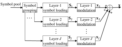
(a) Transmitter.

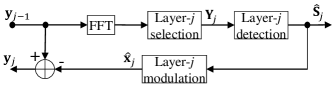
(b) Receiver.

Figure 1: Flowchart of eACO-OFDM transmitter and receiver. Here, $J=2$ in ADO-OFDM and HACO-OFDM, and $J\leq\log\frac{N}{2}$ for LACO-OFDM.

ADO-OFDM

In this scheme, $J=2$ and the second layer employs DCO-OFDM with $\mathcal{K}_{2}=\{k|k\neq\frac{N}{2},k=2(i-1),i\in\{2,\ldots,\frac{N}{2}\}\}$ (even subcarriers). Let ${\mathbf{S}}_{2}={\mathbf{S}}_{\text{dco}}^{(2)}$, where $S_{\text{dco}}^{(2)}(k)$ is a QAM symbol when $k\in\mathcal{K}_{2}$ and $S_{\text{dco}}^{(2)}(k)=0$ otherwise.

Then, ${\mathbf{x}}_{\text{dco}}^{(2)}$ is constructed from ${\mathbf{S}}_{\text{dco}}^{(2)}$ using DCO-OFDM to yield ${\mathbf{x}}_{\text{dco}}^{(2)}=({\mathbf{s}}_{\text{dco}}^{(2)}+d_{\rm dco}^{(2)}\mathbf{1})^{+}$, where ${\mathbf{s}}_{\text{dco}}^{(2)}=\text{IFFT}\{{\mathbf{S}}_{\text{dco}}^{(2)}\}$ and $d_{\rm dco}^{(2)}$ is sufficient large to avoid zero-clipping. Then we have ${\mathbf{x}}_{2}={\mathbf{x}}_{\text{dco}}^{(2)}$ and the ADO-OFDM signal is

$${\color[rgb]{0,0,0}{\mathbf{x}}_{\rm ado}=\sum_{j=1}^{2}{\mathbf{x}}_{j}=\mathbf{x}_{\text{aco}}+\mathbf{x}_{\text{dco}}^{(2)}.}$$

For ADO-OFDM, we have $P_{\text{eff}}=\mathcal{P}\{\frac{\mathbf{s}_{\text{aco}}}{2}+\mathbf{s}_{\text{dco}}^{(2)}\}$. Assuming that $P_{\text{eff}}$ is distributed equally in all effective subcarriers, i.e., $\mathbb{E}[|\frac{S_{\text{aco}}(k_{1})}{2}|^{2}]=\mathbb{E}[|S_{\text{dco}}^{{\color[rgb]{0,0,0}(2)}}(k_{2})|^{2}]$, $\forall k_{1}\in\mathcal{K}_{1},\forall k_{2}\in\mathcal{K}_{2}$, then we have the relations among $P_{\text{elec}}$, $P_{\text{opt}}$, and $P_{\text{eff}}$ as listed in Table I, which are proved in Appendix A.

HACO-OFDM Transmitter

In this scheme, $J=2$ and PAM-DMT is employed in the second layer with $\mathcal{K}_{2}=\{k|k\neq\frac{N}{2},k=2(i-1),i\in\{2,\ldots,\frac{N}{2}\}\}$. Let ${\mathbf{S}}_{2}={\mathbf{S}}_{\text{pam}}^{(2)}$, where $S_{\text{pam}}^{(2)}(k)$ is a PAM symbol when $k\in\mathcal{K}_{2}$ and $S_{\text{pam}}^{(2)}(k)=0$ otherwise. Let ${\mathbf{s}}_{\text{pam}}^{(2)}={\text{IFFT}\{{\mathbf{S}}_{\text{pam}}^{(2)}\}}$ and ${\mathbf{x}}_{\text{pam}}^{(2)}=({{\mathbf{s}}_{\text{pam}}^{(2)}})^{+}$. Then, we have ${\mathbf{x}}_{2}={\mathbf{x}}_{\text{pam}}^{(2)}$ and the HACO-OFDM modulation output is

$${\color[rgb]{0,0,0}{\mathbf{x}}_{\rm haco}=\sum_{j=1}^{2}{\mathbf{x}}_{j}=\mathbf{x}_{\text{aco}}+\mathbf{x}_{\text{pam}}^{(2)}.}$$

For HACO-OFDM, we have $P_{\text{eff}}=\mathcal{P}\{\frac{\mathbf{s}_{\text{aco}}}{2}+\frac{\mathbf{s}_{\text{pam}}^{(2)}}{2}\}$. Assuming that $P_{\text{eff}}$ is distributed equally in all effective subcarriers, i.e., $\mathbb{E}[|\frac{S_{\text{aco}}(k_{1})}{2}|^{2}]=\mathbb{E}[|\frac{S_{\text{pam}}^{(2)}(k_{2})}{2}|^{2}]$, $\forall k_{1}\in\mathcal{K}_{1},\forall k_{2}\in\mathcal{K}_{2}$, then we have the relations between $P_{\text{elec}}$, $P_{\text{opt}}$, and $P_{\text{eff}}$ as listed in Table I, which are proved in Appendix A.

LACO-OFDM Transmitter

In contrast to ADO-OFDM and HACO-OFDM which combine all the muted subcarriers of the first-layer (ACO-OFDM) into a single extra layer (DCO-OFDM layer or PAM-DMT layer, respectivley), LACO-OFDM adopts another ACO-OFDM layer as the second layer, which again leaves some subcarriers unloaded. Then, additional ACO-OFDM layers can be included using the remaining subcarriers [13, 14]. In detail, let $\mathbf{S}_{j}={\mathbf{S}}_{\text{aco}}^{(j)}$, $j=1,\ldots,J$, be the QAM symbols of layer $j$, where ${S}_{\text{aco}}^{(j)}(k)$ is non-zero for $k\in\mathcal{K}_{j}=\{k|k=2^{j-1}(2i-1),i\in\{1,\ldots,\frac{N}{2^{j}}\}\}$ and zero otherwise. This leads to a maximum number of layers $J=\log{\frac{N}{2}}$ for an $N$-subcarrier system. Let ${\mathbf{s}}_{\text{aco}}^{(j)}=\text{IFFT}\{{\mathbf{S}}_{\text{aco}}^{(j)}\}$ and ${\mathbf{x}}_{\text{aco}}^{(j)}=({{\mathbf{s}}_{\text{aco}}^{(j)}})^{+}$. Then, ${\mathbf{x}}_{j}={\mathbf{x}}_{\text{aco}}^{(j)}$ and the overall LACO-OFDM signal is

$${\mathbf{x}}_{\rm laco}=\sum_{j=1}^{J}{{\mathbf{x}}_{j}}=\sum_{j=1}^{J}{{\mathbf{x}}^{(j)}_{\text{aco}}}.$$

For LACO-OFDM, we have $P_{\text{eff}}=\mathcal{P}\{\sum_{j}\frac{\mathbf{s}_{\text{aco}}^{(j)}}{2}\}$. Assuming that $P_{\text{eff}}$ is distributed equally in all effective subcarriers, i.e., $\mathbb{E}[|\frac{S_{\text{aco}}^{(j)}(k)}{2}|^{2}]=\varepsilon$, $\forall j\in\{1,\ldots,J\}$ and $\forall k\in\mathcal{K}_{j}$, for some $\varepsilon$, then we have the relations between $P_{\text{elec}}$, $P_{\text{opt}}$, and $P_{\text{eff}}$ as listed in Table I, which are proved in Appendix A.

II-C2 eACO-OFDM Receiver

A unified receiver for eACO-OFDM is introduced in this part, which applies for ADO-, HACO-, and LACO-OFDM. For the specific receiver of each scheme, the reader is referred to [11, 12, 13]. For convenience, we start the analysis after channel-inversion equalization, and write the received signal as

$${\bf{y}}={\mathbf{x}}+{\mathbf{v}},$$ (3)

where ${\bf{y}}=[y(n)]_{n=1}^{N}$, ${\mathbf{x}}=[x(n)]_{n=1}^{N}$, and ${\mathbf{v}}=[v(n)]_{n=1}^{N}$ is the noise after channel-inversion equalization.

As shown in Fig. 1b, detection is done iteratively, starting with layer $1$ ($j=1$ in Fig. 1b) followed by layers $j=2,3,\ldots$, respectively, until symbols of all layers are detected.

The signal used for detection of symbols in layer $j$ is given by

$${\bf{y}}_{j-1}={\bf{y}}-\sum_{t=1}^{j-1}{\hat{\mathbf{x}}_{t}},$$ (4)

for $j>1$, and by ${\bf{y}}_{0}={\bf{y}}$ for $j=1$. Thus, $\mathbf{y}_{j-1}$ can be understood as the remaining signal after detecting and subtracting layers $1,\ldots,j-1$ and will be used to detect layer $j$.

The signal $\mathbf{y}_{j-1}$ is first transformed to the frequency domain (FFT). Then, the effective subcarriers of layer $j$ are selected (layer-$j$ selection) leading to $\mathbf{Y}_{j}$, and the symbols loaded onto these subcarriers are detected (layer-$j$ detection) leading to $\hat{\mathbf{S}}_{j}$. To remove the contribution of this layer from the subsequent layers, $\hat{\mathbf{S}}_{j}$ is remodulated (layer-$j$ modulation) leading to $\hat{\mathbf{x}}_{j}$, which is then subtracted from $\mathbf{y}_{j-1}$ leading to $\mathbf{y}_{j}$.

This receiver process induces distortion due to residual clipping noise (RCN) as follows. The first ACO-OFDM layer has clipping noise in even subcarriers. This will interfere with the layers $2,\ldots,J$. If $\hat{\mathbf{x}}_{1}$ is not a perfect reconstruction of ${\mathbf{x}}_{1}$ (due to detection errors in layer $1$), then $\mathbf{y}_{1}$ in (4) will contain RCN from the first layer. This will only affect layer 2 in ADO-OFDM and HACO-OFDM. Since LACO-OFDM may have $J>2$ layers of ACO-OFDM, RCN is accumulated layer by layer.

To understand the effects of RCN on the performance of all eACO-OFDM schemes, the next section analyses RCN in detail.

III Analysis on Residual Clipping Noise

In this section, we analyse RCN by deriving its mathematical expression, proving some statistical properties, and then using these to model the power of RCN in each layer, which enables the estimation of RCN power and total noise power in each subcarrier.

III-A Mathematical Expression of RCN and Total Noise

In the eACO-OFDM receiver, the output of the detection process in Fig. 1b can be written as

$$\hat{\mathbf{S}}_{j}={\mathbf{S}}_{j}+{\mathbf{E}}_{j},$$ (5)

where ${\mathbf{E}}_{j}=[E_{j}(k)]_{k=0}^{N-1}$ and $E_{j}(k)$ is the detection-error in subcarrier $k$ of layer $j$. In the time domain, we have $\hat{\mathbf{s}}_{j}={\mathbf{s}}_{j}+{\mathbf{e}}_{j}$, where $\hat{\mathbf{s}}_{j}=\text{IFFT}\{\hat{\mathbf{s}}_{j}\}$ and ${\mathbf{e}}_{j}=\text{IFFT}\{{\mathbf{E}}_{j}\}$. Since the first layer is an ACO-OFDM layer, then $\hat{\mathbf{x}}_{1}$ is given by

$$\hat{\mathbf{x}}_{1}=(\hat{\mathbf{s}}_{1})^{+}=\frac{1}{2}({\mathbf{s}}_{1}+{\mathbf{e}}_{1}+|{\mathbf{s}}_{1}+{\mathbf{e}}_{1}|).$$ (6)

Then, from (4), the second iteration at the receiver starts from

$${\bf{y}}_{1} =\sum_{t=1}^{J}{\mathbf{x}}_{t}+{\mathbf{v}}-\hat{\mathbf{x}}_{1}$$

$$=\sum_{t=2}^{J}{\mathbf{x}}_{t}+{\mathbf{v}}+\frac{1}{2}({\mathbf{s}}_{1}+|{\mathbf{s}}_{1}|)-\frac{1}{2}({\mathbf{s}}_{1}+{\mathbf{e}}_{1}+|{\mathbf{s}}_{1}+{\mathbf{e}}_{1}|)$$

$$=\sum_{t=2}^{J}{\mathbf{x}}_{t}+{\mathbf{v}}-\frac{1}{2}{\mathbf{e}}_{1}+\frac{1}{2}(|{\mathbf{s}}_{1}|-|{\mathbf{s}}_{1}+{\mathbf{e}}_{1}|).$$ (7)

In (III-A), $\bf{v}$ interferes with all layers; $\frac{1}{2}{\bf{e}}_{1}$ has a frequency-domain counterpart $\frac{1}{2}\mathbf{E}_{1}$ which is only nonzero in the effective subcarriers of layer 1 (odd sybcarriers), and thus will not interfere with layers higher than 1. The term $\frac{1}{2}(|{\mathbf{s}}_{1}|-|{\mathbf{s}}_{1}+{\mathbf{e}}_{1}|)$ is the RCN which interferes with layers $j>1$.

To generalize this, consider iteration $j+1$ at the receiver. From (4), this iteration starts from

$${\bf{y}}_{j} =\sum_{t=1}^{J}{{\mathbf{x}}_{t}}+{\mathbf{v}}-\sum_{t=1}^{j}{\hat{\mathbf{x}}_{t}}$$

$$=\sum_{t>j}^{J}{{\mathbf{x}}_{t}}+{\mathbf{v}}-\frac{1}{2}\sum_{t=1}^{j}{{\mathbf{e}}_{t}}+\sum_{t=1}^{j}{\frac{1}{2}(|{\mathbf{s}}_{t}|-|{\mathbf{s}}_{t}+{\mathbf{e}}_{t}|)}.$$ (8)

In (III-A), $\frac{1}{2}\sum_{t=1}^{j}{{\mathbf{e}}_{t}}$ is the time-domain error signal induced by the detection errors in layers $1,\ldots,j$, whose frequency-domain counterpart is nonzero only in the effective subcarriers of layers $1,\ldots,j$, and thus does not interfere with layers $j+1,\ldots,J$. The term $\sum_{t=1}^{j}{\frac{1}{2}(|{\mathbf{s}}_{t}|-|{\mathbf{s}}_{t}+{\mathbf{e}}_{t}|)}$ in (III-A) is the RCN caused by layers $1,\ldots,j$, which interferes with all layers $j+1,\ldots,J$. For convenience, we denote the RCN from layer $t$ as

$${\bm{\delta}}_{t}={\frac{1}{2}(|{\mathbf{s}}_{t}|-|{\mathbf{s}}_{t}+{\mathbf{e}}_{t}|)}.$$ (9)

Note that $|\delta_{t}(n)|\leq\frac{1}{2}|e_{t}(n)|$ which can be shown using the reverse triangle inequality.

Using this, we can write the total noise after removing layer $j$ as

$${\bf{z}}_{j}={\mathbf{v}}+\sum_{t=1}^{j}{{\bm{\delta}}_{t}},$$ (10)

for $j>0$, and ${\bf{z}}_{0}={\mathbf{v}}$ for $j=0$.

Note that the total noise expression (10) applies for the three eACO-OFDM schemes, with $j\in\{0,1\}$ for ADO-OFDM and HACO-OFDM; and $j\in\{0,\ldots,J-1\}$ for LACO-OFDM. Next, we study some statistical properties of RCN, which are useful for modeling the RCN power.

III-B Statistical Properties of RCN

RCN $\bm{\delta}_{t}$ and noise $\mathbf{v}$ result in detection errors. The error rate can be evaluated analytically for a given QAM constellation if the statistics of total noise is known [26]. This necessitates studying the statistics of RCN. In this section, we provide three statistical properties of RCN which will facilitate error rate evaluation of eACO-OFDM (discussed next section).

First, we state two lemmas which are required to prove statistical properties of RCN, and can be proved using the Lyapunov central limit theorem [27, Example 27.4].

Lemma 1.

Consider $N$ complex-valued random variables $X(k)$, $k=0,1,\ldots,N-1$, that satisfy $\mathbb{E}[X(k)]=0$ and $|X(k)|\leq K<\infty$ $\forall k$, where $K$ is a constant, and Hermitian symmetry, i.e., $X(k)=X^{*}(N-k)$ for $0<k<\frac{N}{2}$. Let $\mathbb{V}[X(k)]=\sigma_{X}^{2}(k)$ and $x(n)=\frac{1}{N}\sum_{k=0}^{N-1}X(k)e^{\mathsf{j}\frac{2\pi}{N}kn}$. Then $x(n)\xrightarrow{d}\mathcal{N}\big{(}0,\frac{1}{N^{2}}\sum_{k=0}^{N-1}\sigma_{X}^{2}(k)\big{)}$ as $N\rightarrow\infty$.

Lemma 2.

Consider $N$ i.i.d. real-valued random variables $x(n)$, $n=0,1,\dots,N-1$, that have mean $\mu_{x}$, variance $\sigma_{x}^{2}$, and satisfy $|x(n)|\leq A<\infty$ $\forall n$, where $A$ is a constant. Let $X(k)=\sum_{n=0}^{N-1}x(n)e^{-\mathsf{j}\frac{2\pi}{N}kn}$. Then, $X(k)\xrightarrow{d}\mathcal{CN}(0,N\sigma_{x}^{2})$ when $N\rightarrow\infty$ $\forall k\notin\{0,\frac{N}{2}\}$, and $X(\frac{N}{2})\xrightarrow{d}\mathcal{N}(0,N\sigma_{x}^{2})$.

Now let ${\bm{\Delta}}_{t}=[\Delta_{t}(k)]_{k=0}^{N-1}=\text{FFT}\{\bm{\delta}_{t}\}$ and ${\mathbf{E}}_{t}=[E_{t}(k)]_{k=0}^{N-1}=\text{FFT}\{\mathbf{e}_{t}\}$ be the IFFT of $\bm{\delta}_{t}$ and $\mathbf{e}_{t}$, respectively, and let $\mathcal{B}_{t}\triangleq\{k|k=2^{t-1}2(i-1),i\in\{1,\ldots,\frac{N}{2^{t}}\},k\neq 0,k\neq\frac{N}{2}\}$ denote the set of subcarriers affected by RCN from layer $t$. Then for an eACO-OFDM system with Gaussian noise, channel-inversion equalization, QAM and ML-detection, we have the following three properties of RCN:

1. When $|\mathcal{K}_{t}|$ is large enough, the time-domain RCN $\delta_{t}(n)$ is independent and identical distributed (i.i.d.) with respect to $n$;

2. When $|\mathcal{K}_{t}|$ is large enough, the frequency-domain RCN $\Delta_{t}(k)\xrightarrow{d}\mathcal{CN}(0,N{\color[rgb]{0,0,0}\sigma_{\delta_{t}}^{2}})$, for all $k\in\mathcal{B}_{t}$, where $\sigma_{\delta_{t}}^{2}=\mathbb{V}[\delta_{t}(n)]$ which is independent of $n$ by property 1;

3. The covariance of the frequency-domain RCN from layers $t_{1}$ and $t_{2}$ is negligible for any $k$ and $t_{2}\neq t_{1}$. Since $\mathbb{E}\{\Delta_{t}(k)\}{\color[rgb]{0,0,0}=}0$ by property 2, this implies that $\mathbb{E}\{\Delta_{t_{1}}(k)\Delta_{t_{2}}^{*}(k)\}\approx 0$.

The first two properties can be proved using Lemmas 1 and 2. The third property will not be proved, but is supported by simulations.

Proof of Property 1 and 2: First recall from the definition of the time-domain RCN in (9) that ${\bm{\delta}}_{t}={\frac{1}{2}(|{\mathbf{s}}_{t}|-|{\mathbf{s}}_{t}+{\mathbf{e}}_{t}|)}$. The proof follows five steps which show that (i) $s_{t}(n)$ is i.i.d. Gaussian, (ii) $e_{1}(n)$ is i.i.d. Gaussian, (iii) $\delta_{1}(n)$ is i.i.d., and (iv) $\Delta_{1}(k)$ is zero-mean circularly-symmetric complex Gaussian identically $\forall k\in\mathcal{B}_{1}$. Then, we use these steps to prove properties 1 and 2 by induction.

Step (i): As QAM symbols are transmitted on $S_{t}(k)$ equiprobably for $k\in\mathcal{K}_{t}$ and $S_{t}(k)=0$ $\forall k\notin\mathcal{K}_{t}$, it follows that $S_{t}(k)$ has zero-mean and is bounded. Moreover, $\mathbf{S}_{t}$ has Hermitian-symmetry. Then it follows from Lemma 1 that $s_{t}(n)\xrightarrow{d}\mathcal{N}\big{(}0,\frac{1}{N^{2}}\sum_{k=0}^{N-1}\mathbb{V}[S_{t}(k)]\big{)}$ as $|\mathcal{K}_{t}|\rightarrow\infty$ for all $n$. Moreover, due to the approximate orthogonality of the vectors $[e^{\mathsf{j}\frac{2\pi}{N}kn_{1}}]_{k=0}^{N-1}$ and $[e^{\mathsf{j}\frac{2\pi}{N}kn_{2}}]_{k=0}^{N-1}$ when $N\rightarrow\infty$ (which holds if $|\mathcal{K}_{t}|\to\infty$), it follows that $s_{t}(n_{1})$ and $s_{t}(n_{2})$ are independent, $\forall$ $n_{1}\neq n_{2}$ when $|\mathcal{K}_{t}|$ is large.

Step (ii): From (5), we have that $E_{1}(k)=\hat{S}_{1}(k)-S_{1}(k)$ for $k\in\mathcal{K}_{1}$ and $E_{1}(k)=0$ otherwise, where $\hat{S}_{1}(k)$ is the detection outcome of $S_{1}(k)$. Since $\mathbf{S}_{1}$ is Hermitian-symmetric, and the real-valued time-domain noise has a Hermitian-symmetric frequency-domain counterpart, it follows that $\hat{\mathbf{S}}_{1}$ is Hermitian-symmetric, and hence $\mathbf{E}_{1}$ is also Hermitian-symmetric. Note also that since $\hat{S}_{1}(k)$ and $S_{1}(k)$ are bounded (bounded QAM constellation), then $E_{1}(k)$ is also bounded. Now since $Z_{0}(k)=V(k)$ (cf. (10)) has zero-mean and a symmetric probability density function, then $E_{1}(k)$ has zero-mean. Using Lemma 1, we conclude that $e_{1}(n)\xrightarrow{d}\mathcal{N}\big{(}0,\frac{1}{N^{2}}\sum_{k=0}^{N-1}\mathbb{V}[E_{1}(k)]\big{)}$ as $|\mathcal{K}_{1}|\rightarrow\infty$ for any $n$. The independence between $e_{1}(n_{1})$ and $e_{1}(n_{2})$, $\forall$ $n_{1}\neq n_{2}$ when $N\rightarrow\infty$ can be proved similar to $s_{t}(n)$ in the previous paragraph.

Step (iii): Note that $\delta_{1}(n)=\frac{1}{2}(|s_{1}(n)|-|s_{1}(n)+e_{1}(n)|)$, where $s_{1}(n)$ and $e_{1}(n)$ are respectively i.i.d. (from (i) and (ii)). Moreover, the independence of $s_{1}(n_{1})$ and $e_{1}(n_{2})$ for any $n_{1}\neq n_{2}$ when $N\rightarrow\infty$ can be proved similar to $s_{t}(n)$ in step (i). Thus, $\delta_{1}(n)$ is i.i.d.. Denote its variance by $\sigma_{\delta_{1}}^{2}$.

Step (iv): For $k\in\mathcal{B}_{1}$, $\Delta_{1}(k)=\sum_{n=0}^{N-1}{\delta_{1}(n)e^{-\mathsf{j}\frac{2\pi}{N}kn}}$, where $\delta_{1}(n)$ is i.i.d. (cf. step (iii)). Since $|\delta_{1}(n)|\leq\frac{1}{2}|e_{1}(n)|$ (cf. (9)) and $e_{1}(n)$ is a Gaussian random variable with small variance for large $|\mathcal{K}_{1}|$ (cf. proof of (ii)), then $|\delta_{1}(n)|$ is bounded for large $|\mathcal{K}_{1}|$. Thus, from Lemma 2, we have $\Delta_{1}(k)\xrightarrow{d}\mathcal{CN}(0,N{\color[rgb]{0,0,0}\sigma_{\delta_{1}}^{2}})$ as $|\mathcal{K}_{1}|\to\infty$ for all $k\in\mathcal{B}_{1}$.

Now the above steps can be used to prove properties 1 and 2 by induction. Since $\Delta_{1}(k)$ is zero-mean Gaussian for $k\in\mathcal{B}_{t}$ (iv), then $Z_{t}(k)=V(k)+\sum_{i=1}^{t}\Delta_{i}(k)$ with $t=1$ is zero-mean Gaussian for $k\in\mathcal{B}_{1}$. Following the same lines of steps (ii), (iii), and (iv), it follows that $\delta_{2}(n)$ is i.i.d. and $\Delta_{2}(k)$ is zero-mean Gaussian for $k\in\mathcal{B}_{2}$. Repeating these steps for all $t=2,3,\ldots$ with $|\mathcal{K}_{t}|$ large proves properties 1 and 2.

Evidence of Property 3: We do not provide a formal proof of property 3, but rather an intuitive explanation supported by numerical simulations in Fig. 3. As system noise $\mathbf{v}$ is always the major stimulator of detection errors, then ${\Delta}_{t}(k)$ depends more on system noise than on RCN from lower layers. Since system noise is independent across layers, ${\Delta}_{t}(k)$ will be almost independent across layers. Fig. 4 shows that system noise power is much larger than RCN power for a wide range of SNR. This supports property 3.

Remark 1.

Properties 1-3 do not require equal bit-loading and uniform noise power spectrum.

Remark 2.

Properties 1-3 are only exact asymptotically when $|\mathcal{K}_{t}|\rightarrow\infty$, and become less precise when $|\mathcal{K}_{t}|$ is small. Nevertheless, the approximation is still acceptable for small $|\mathcal{K}_{t}|$ as shown in Fig. 2, 4, and 5.

Remark 3.

Note that we also have $\Delta_{t}(\frac{N}{2})\xrightarrow{d}\mathcal{N}(0,N\sigma_{\delta_{t}}^{2})$ which can be proved by Lemma 2. Moreover, as $\delta_{t}(n)$ is i.i.d., it is straightforward to prove that $\Delta_{t}(0)=\sum_{n=0}^{N-1}\delta_{t}(n)$ satisfies $\mathbb{E}[\Delta_{t}(0)]=N\mathbb{E}[\delta_{t}(n)]$ and $\mathbb{V}[\Delta_{t}(0)]=N{\color[rgb]{0,0,0}\sigma_{\delta_{t}}^{2}}$ which is equal to $\mathbb{V}[\Delta_{t}(k)]$, $\forall k\in\mathcal{B}_{t}\cup\{\frac{N}{2}\}$. This will be needed in Sec. III-C.

III-C Worst-case RCN Power Model

Recall that $|{\delta}_{t}(n)|\leq\frac{1}{2}|e_{t}(n)|$, which implies

$$\mathcal{P}\{\bm{\delta}_{t}\}\leq\frac{1}{4}\mathcal{P}\{\mathbf{e}_{t}\}=\frac{1}{4N}\mathcal{P}\{\mathbf{E}_{t}\}=\frac{1}{4N^{2}}\sum_{k=0}^{N-1}\mathcal{P}\{E_{t}(k)\},$$ (11)

from Parseval’s theorem. This forms a worst-case model for the power of the time-domain RCN $\mathcal{P}\{\bm{\delta}_{t}\}$ in terms of $\mathcal{P}\{E_{t}(k)\}$. A worst-case model of the power of the frequency-domain RCN can be obtained using $\mathcal{P}\{\bm{\Delta}_{t}\}=N\mathcal{P}\{\bm{\delta}_{t}\}$ from Parsevel’s theorem. It remains to derive a worst-case model of the power of the frequency-domain RCN per subcarrier, i.e., $\Delta_{t}(k)$.

Using Remark 3 and property 2, we have $\mathcal{P}\{\Delta_{t}(0)\}=\mathbb{V}[\Delta_{t}(0)]+\mathbb{E}^{2}\{\Delta_{t}(0)\}\geq\mathbb{V}[\Delta_{t}(k)]=\mathcal{P}\{\Delta_{t}(k)\}$ for any $k\in\mathcal{B}_{t}$. Thus, $\mathcal{P}\{\Delta_{t}(0)\}\geq\mathcal{P}\{\Delta_{t}(\frac{N}{2})\}=\mathcal{P}\{\Delta_{t}(k)\}$ for any $k\in\mathcal{B}_{t}$. Moreover, $\mathcal{P}\{\Delta_{t}(k)\}=0$ for $k\notin\mathcal{B}_{t}\cup\{0,\frac{N}{2}\}$. Using these, and since $\Delta_{t}(k)$ is i.i.d. for $k\in\mathcal{B}_{t}$ (property 2), then $\mathcal{P}\{\bm{\Delta}_{t}\}=\frac{1}{N}(\mathcal{P}\{\Delta_{t}(0)\}+(|\mathcal{B}_{t}|+1)\mathcal{P}\{\Delta_{t}(k)\})\geq\frac{|\mathcal{B}_{t}|+2}{N}\mathcal{P}\{\Delta_{t}(k)\}$ for any $k\in\mathcal{B}_{t}$. Then, since $\mathcal{P}\{\bm{\Delta}_{t}\}=N\mathcal{P}\{\bm{\delta}_{t}\}$, we obtain the following for $k\in\mathcal{B}_{t}$

$$\mathcal{P}\{\Delta_{t}(k)\}\leq\frac{N^{2}}{|\mathcal{B}_{t}|+2}\mathcal{P}\{\bm{\delta}_{t}\}\leq\frac{N^{2}}{|\mathcal{B}_{t}|+2}\frac{1}{4N^{2}}\sum_{\tilde{k}=0}^{N-1}\mathcal{P}\{E_{t}(\tilde{k})\}=\frac{1}{4|\mathcal{K}_{t}|}\sum_{\tilde{k}\in\mathcal{K}_{t}}\mathcal{P}\{E_{t}(\tilde{k})\},$$ (12)

where the last equality follows since $\mathcal{P}\{E_{t}(k)\}=0$ for $k\notin\mathcal{K}_{t}$ and since $|\mathcal{K}_{t}|=|\mathcal{B}_{t}|+2$. This provides a worst-case estimation of $\mathcal{P}\{\Delta_{t}(k)\}$ in terms of the detection error power $\mathcal{P}\{E_{t}(k)\}$. Next, we relate $\mathcal{P}\{E_{t}(k)\}$ with the QAM constellation and noise power using the following definition.

Definition 1.

For a complex AWGN channel $Y=X+Z$ with input $X$ uniformly distributed over an $M$-QAM constellation with a minimum Euclidean distance $d_{\text{min}}$, Gaussian noise $Z$ with variance $\sigma^{2}$, and detection outcome $\hat{X}$, let $\mathsf{f}(d_{\text{min}},\sigma^{2},M)$ be a function which maps $(d_{\text{min}},\sigma^{2},M)$ to a real number which equals the power of detection errors over this channel, i.e., $\mathsf{f}(d_{\text{min}},\sigma^{2},M)=\mathbb{E}\{|X-\hat{X}|^{2}\}$.

A method for approximating $\mathsf{f}(d_{\text{min}},\sigma^{2},M)$ is described in Appendix B and will be used in the simulations.

Denote the QAM constellation size used in subcarrier $k$ of layer $t$ by $M_{t}(k)$. Suppose that before detection, ${\bf{Y}}_{j}$ is scaled by 2 to recover the original scale of the constellation before clipping. Then, the power of noise in subcarrier $k$ of layer $t$ becomes $4\mathcal{P}\{Z_{t-1}(k)\}$ (to be derived in the next subsection). The minimum Euclidean distance of the constellation in subcarrier $k$ can be written as [26]

$$d_{t}(k)=\sqrt{\frac{6\mathcal{P}\{S_{t}(k)\}}{M_{t}(k)-1}}.$$ (13)

Note that (13) is only accurate for square QAM constellations or rectangular QAM constellations with a large constellation size [26]. Using Definition 1, we have

$$\mathcal{P}\{E_{t}(k)\}={\color[rgb]{0,0,0}\mathsf{f}}\big{(}d_{t}(k),{\color[rgb]{0,0,0}4}\mathcal{P}\{Z_{t-1}(k)\},M_{t}(k)\big{)}.$$ (14)

Then from (12), we have

$$\mathcal{P}\{{{\Delta}}_{t}(k)\}\leq P_{t}^{\rm w}\triangleq\frac{1}{4{\color[rgb]{0,0,0}|\mathcal{K}_{t}|}}{\color[rgb]{0,0,0}\sum_{{\color[rgb]{0,0,0}\tilde{k}}\in\mathcal{K}_{t}}}{{\color[rgb]{0,0,0}\mathsf{f}}\big{(}d_{t}(\tilde{k}),{\color[rgb]{0,0,0}4}\mathcal{P}\{Z_{t-1}(\tilde{k})\},M_{t}(\tilde{k})\big{)}},$$ (15)

where $P_{t}^{\rm w}$ represents the worst-case RCN power. For each $t$, $P_{t}^{\rm w}$ is the same for $k\in\mathcal{B}_{t}$ and is always 0 for $k\notin\mathcal{B}_{t}$.

III-D Worst-Case Total Noise Power

The frequency-domain counterpart of (10) is

$$Z_{j}(k)={V(k)}+\sum_{t=1}^{j}{{\Delta}_{t}(k)},\;\;j>0,$$ (16)

Thus,

$$\mathcal{P}\{Z_{j}(k)\}=\mathbb{E}[{Z_{j}(k)}{Z_{j}^{*}(k)}]=\mathbb{E}\big{[}[{V(k)}+\sum_{t=1}^{j}{{\Delta}_{t}(k)}][{V(k)}+\sum_{t=1}^{j}{{\Delta}_{t}(k)}]^{*}\big{]}.$$ (17)

Since ${\Delta}_{t}(k)$ is RCN from layer $t-1$ and $V(k)$ is noise in layer $t$, ${\Delta}_{t}(k)$ is independent of $V(k)$ for $k\in\mathcal{B}_{t}$. Also, $\mathbb{E}[\Delta_{t_{1}}(k)\Delta_{t_{2}}^{*}(k)]\approx 0$ for $t_{1}\neq t_{2}$ (Property 3). Then, (17) can be written as

$$\mathcal{P}\{Z_{j}(k)\}=\mathcal{P}\{V(k)\}+\sum_{t=1}^{j}{\mathcal{P}\{{\Delta}_{t}(k)\}{\color[rgb]{0,0,0}\leq\mathcal{P}\{V(k)\}+\sum_{t=1}^{j}{P_{t}^{\rm w}}}},$$ (18)

where the last inequality follows from (15).

Now, using (15) and (18), we can upper bound the RCN power $\mathcal{P}\{{{\Delta}}_{t}(k)\}$ and the total noise power $\mathcal{P}\{Z_{j}(k)\}$. The bounds can be used to obtain worst-case values of RCN and total noise power iteratively, as follows. For $t=0$, we have $P_{0}^{\rm w}=0$ and $\mathcal{P}\{Z_{0}(k)\}=\mathcal{P}\{V(k)\}$. Consequently, for $t=1$, we obtain $P_{1}^{\rm w}=\frac{1}{2N}\sum_{k\in\mathcal{K}_{1}}\mathsf{f}\big{(}d_{1}(k),{\color[rgb]{0,0,0}4}\mathcal{P}\{V(k)\},M_{1}(k)\big{)}$ and $\mathcal{P}\{Z_{1}(k)\}\leq\mathcal{P}\{V(k)\}+P_{1}^{\rm w}$. Using $P_{1}^{\rm w}$ and $\mathcal{P}\{V(k)\}+P_{1}^{\rm w}$ as worst-case RCN and total noise powers, respectively, we obtain $P_{2}^{\rm w}=\frac{1}{N}\sum_{k\in\mathcal{K}_{2}}\mathsf{f}\big{(}d_{2}(k),4(\mathcal{P}\{V(k)\}+P_{1}^{\rm w}),M_{2}(k)\big{)}$ and $\mathcal{P}\{Z_{2}(k)\}\leq\mathcal{P}\{V(k)\}+P_{1}^{\rm w}+P_{2}^{\rm w}$ for $t=2$, and so on.

The quality of this worst-case RCN power model will be evaluated in Sec. VI-C. In the following sections, we use the RCN power model for performance analysis and system optimization of eACO-OFDM.

IV Symbol Error Probability of eACO-OFDM

In this section, we derive the theoretical symbol error probabilities of the three eACO-OFDM schemes assuming an AWGN channel and ML detection, while taking RCN into account.

Given an arbitrary $M$-QAM or $M$-PAM symbol of average power $\varepsilon$ transmitted through an AWGN channel with noise variance $\sigma^{2}$, and given a receiver which adopts ML detection, the symbol error rate is given by [26]

$$\mathsf{p}_{\rm e}^{\rm QAM}(M,\varepsilon,\sigma^{2}) =4\frac{\sqrt{M}-1}{\sqrt{M}}\mathsf{Q}\left(\frac{\sqrt{3\varepsilon}}{\sqrt{M-1}\sigma}\right)\cdot\left[1-\frac{\sqrt{M}-1}{\sqrt{M}}\mathsf{Q}\left(\frac{\sqrt{3\varepsilon}}{\sqrt{M-1}\sigma}\right)\right],$$ (19)

$$\mathsf{p}_{\rm e}^{\rm PAM}(M,\varepsilon,\sigma^{2}) =2\frac{\sqrt{M}-1}{\sqrt{M}}\mathsf{Q}\left(\frac{\sqrt{6\varepsilon}}{\sqrt{M^{2}-1}\sigma}\right),$$ (20)

Using these expressions, and the worst-case RCN power model from last section, we can evaluate the performance of eACO-OFDM schemes as described next.

IV-A ADO-OFDM

Both layers of ADO-OFDM use QAM. Denote the constellation size of subcarrier $k$ of layer $j$ by $M_{j}(k)$. In the first layer, the signal amplitude is halved because of clipping, and hence $\varepsilon$ in (19) is equal to $\frac{\mathcal{P}\{S_{1}(k)\}}{4}$. Also, the total noise power is $\mathcal{P}\{V(k)\}$. Thus the error probability is

$$p_{\rm e,1}^{\rm ado}(k)=\mathsf{p}_{\rm e}^{\rm QAM}\left(M_{1}(k),\frac{\mathcal{P}\{S_{1}(k)\}}{4},\mathcal{P}\{V(k)\}\right).$$ (21)

In the second layer, $\varepsilon$ in (19) is equal to $\mathcal{P}\{S_{2}(k)\}$ since there is no clipping, and the total noise power is $\mathcal{P}\{Z_{1}(k)\}\leq\mathcal{P}\{V(k)\}+P_{1}^{\rm w}$ by (18). Thus the error probability is

$$p_{\rm e,2}^{\rm ado}(k) =\mathsf{p}_{\rm e}^{\rm QAM}\big{(}M_{2}(k),\mathcal{P}\{S_{2}(k)\},\mathcal{P}\{Z_{1}(k)\}\big{)}$$

$$\leq\mathsf{p}_{\rm e}^{\rm QAM}\big{(}M_{2}(k),\mathcal{P}\{S_{2}(k)\},\mathcal{P}\{V(k)\}+P_{1}^{\rm w}\big{)}.$$ (22)

Denote the number of loaded effective subcarriers in all layers by $N^{\prime}\leq N-2$. Then, the overall error probability is the average of the error probabilities of all effective subcarriers, i.e.,

$$p_{\rm e}^{\rm ado}=\frac{\sum_{j=1,2}\sum_{k}{p_{{\rm e},j}^{\rm ado}(k)}}{N^{\prime}}.$$ (23)

IV-B HACO-OFDM

The two layers of HACO-OFDM use QAM and PAM respectively. Both layers have clipping, which halves the signal amplitude leading to $\varepsilon=\frac{\mathcal{P}\{S_{j}(k)\}}{4}$ in (19) and (20). The noise power in layers 1 and 2 is $\mathcal{P}\{V(k)\}$ and $\mathcal{P}\{Z_{1}(k)\}\leq\mathcal{P}\{V(k)\}+P_{1}^{\rm w}$ (using (18)), respectively. Thus the error probabilities of the two layers are

$$p_{\rm e,1}^{\rm haco}(k) =\mathsf{p}_{\rm e}^{\rm QAM}\left(M_{1}(k),\frac{\mathcal{P}\{S_{1}(k)\}}{4},\mathcal{P}\{V(k)\}\right),$$ (24)

$$p_{\rm e,2}^{\rm haco}(k) =\mathsf{p}_{\rm e}^{\rm PAM}\left(M_{2}(k),\frac{\mathcal{P}\{S_{2}(k)\}}{4},\mathcal{P}\{Z_{1}(k)\}\right)$$

$${\color[rgb]{0,0,0}\leq\mathsf{p}_{\rm e}^{\rm PAM}\left(M_{2}(k),\frac{\mathcal{P}\{S_{2}(k)\}}{4},\mathcal{P}\{V(k)\}+P_{1}^{\rm w}\right).}$$ (25)

The overall error probability is

$$p_{\rm e}^{\rm haco}=\frac{\sum_{j=1,2}\sum_{k}{p_{{\rm e},j}^{\rm haco}(k)}}{N^{\prime}},$$ (26)

where $N^{\prime}$ is the number of loaded effective subcarriers in all layers.

IV-C LACO-OFDM

Each layer uses QAM and has clipping, which halves the signal amplitude. This leads to $\varepsilon=\frac{\mathcal{P}\{S_{j}(k)\}}{4}$ in (19). Also, the total noise power is $\mathcal{P}\{V(k)\}$ in layer 1 and $\mathcal{P}\{Z_{j}(k)\}\leq\mathcal{P}\{V(k)\}+\sum_{t=1}^{j-1}P_{j}^{\rm w}$ in layer $j+1$, $j\in\{1,\ldots,J-1\}$ (using (18)). Thus the error probability of layer $j$ is

$$p_{{\rm e},j}^{\rm laco}(k) =\mathsf{p}_{\rm e}^{\rm QAM}\left(M_{j}(k),\frac{\mathcal{P}\{S_{j}(k)\}}{4},\mathcal{P}\{Z_{j-1}(k)\}\right)$$

$$\leq\mathsf{p}_{\rm e}^{\rm QAM}\left(M_{j}(k),\frac{\mathcal{P}\{S_{j}(k)\}}{4},\mathcal{P}\{V(k)\}+\sum_{t=1}^{j-1}P_{t}^{\rm w}\right).$$ (27)

The overall error probability is

$$p_{\rm e}^{\rm laco}=\frac{\sum_{j}\sum_{k}{p_{{\rm e},j}^{\rm laco}(k)}}{N^{\prime}},$$ (28)

where $N^{\prime}$ is the number of loaded effective subcarriers in all layers.

Now we are able to evaluate the SER of the eACO-OFDM schemes with higher accuracy since the RCN is included in the expression. The quality of this evaluation is shown numerically in Sec. VI-D. Next, we show how these results can be used for RCN-aware system optimization.

V RCN-Aware System Optimization

In this section, we discuss an exemplary RCN-aware resource-allocation application, that serves to demonstrate the usefulness of the RCN model for designing a reliable LACO-OFDM scheme in the presence of RCN without using multi-class coding.

Since RCN is accumulated layer by layer in LACO-OFDM, subcarriers from different layers are distorted by different levels of RCN power. This affects the optimization of bit loading and power allocation. If RCN is not taken into account in this optimization, the scheme may fail to deliver the expected performance. Using the proposed RCN power model, we propose an RCN-aware SER-controlled LACO-OFDM design which makes the scheme more reliable.

We consider a bit-rate maximization problem (BRMP) in LACO-OFDM, where the allocated power and bits of each subcarrier are adaptively changed according to the channel condition, to meet power and error rate constraints. Under these assumptions, we propose an RCN-aware iterative algorithm for bit loading and power allocation. Denote the number of bits loaded into subcarrier $k$ by $B(k)$, the effective power allocated to subcarrier $k$ by $P_{s}(k)$, i.e., $\mathcal{P}\{\frac{S_{j}(k)}{2}\}=P_{s}(k)$, and the ‘effective power’ budget by $P_{\rm eff}$, which can be obtained from the electrical power budget $P_{\text{elec}}$ or optical power budget $P_{\text{opt}}$ using Table I. Also, denote the worst-case total noise power of each subcarrier by $P_{z}(k)$, which is initialized to $P_{z}^{(0)}(k)=\mathcal{P}\{Z_{0}(k)\}=\mathcal{P}\{V(k)\}$ at iteration $i=0$. Then, $B(k)$, $P_{s}(k)$ and $P_{z}(k)$ are updated iteratively as follows.

1. Set $i=0$, and $\Phi=\{1,\ldots,N-1\}$.

2. Calculate $P_{s}^{(i)}(k)$, $k\in\Phi$, by solving $\max_{P_{s}^{(i)}(k)}\sum_{k\in\Phi}\log\left(1+\frac{|H(k)|^{2}P_{s}^{(i)}(k)}{P_{z}^{(i)}(k)}\right)$ subject to $\sum_{k\in\Phi}P_{s}^{(i)}(k)\leq N^{2}P_{\text{eff}}$, where $H(k)$ is the channel magnitude in subcarrier $k$.

3. Set $B^{(i)}(k)=\lfloor R_{\Gamma}(k)\rfloor$, $k\in\Phi$, where $R_{\Gamma}(k)=\log\left(1+\frac{|H(k)|^{2}P_{s}^{(i)}(k)}{\mathsf{\Gamma}(p_{\rm e})P_{z}^{{(i)}}(k)}\right)$, $p_{\rm e}$ is a given SER constraint, and $\mathsf{\Gamma}(p_{\rm e})=\frac{1}{3}\left[Q^{-1}\left(\frac{1}{4}p_{\rm e}\right)\right]^{2}$ [28].

4. If $B^{(i)}(k)=0$ for some $k\in\Phi$, update $\Phi$ to $\Phi\setminus\{k|B^{(i)}(k)=0\}$ and repeat from step 2.

5. Calculate $P_{z}^{(i+1)}(k)$ for all $k$ using (18), i.e., $P_{z}^{(i+1)}(k)=\mathcal{P}\{V(k)\}+\sum_{t=1}^{j_{k}-1}P_{t}^{\rm w}$ where $j_{k}$ is the index of the layer which contains effective subcarrier $k$, i.e., $k\in\mathcal{K}_{j_{k}}$. To calculate $P_{t}^{\rm w}$, use (15) with $M_{t}(k)=2^{B^{(i)}(k)}$ and $\mathcal{P}\{S_{t}(k)\}=4P_{s}^{(i)}(k)$.

6. If $\|{\bf{P}}_{z}^{(i+1)}-{\bf{P}}_{z}^{(i)}\|^{2}>\epsilon$ where $\epsilon\ll\frac{\|{\bf{P}}_{z}^{(i)}\|^{2}}{N}$ and ${\bf{P}}_{z}^{(i)}=[P_{z}^{(i)}(k)]_{k=0}^{N-1}$, increment $i$, set $\Phi=\{1,\ldots,N-1\}$, and repeat from step 2, otherwise, end the algorithm.

If RCN power is perfectly estimated, then the bit loading scheme from step 3 will be able to maintain the SER below $p_{\rm e}$. Sec. VI-E shows simulation results of the proposed SER-controlled LACO-OFDM scheme, and it also shows that the number of iterations required in the optimization is small.

VI Simulations and Discussions

In this section, we use simulations to examine the main conclusions of the former sections. In all the following simulations, $N=1024$ and $\mathcal{P}\{{\mathbf{v}}\}=1$. All the available subcarriers are used to transmit information, which means LACO-OFDM has $9$ layers. Monte-Carlo simulation uses $10^{4}$ independent runs, and in each run, information symbols and noise are generated randomly. Define $\gamma=10\log_{10}\frac{P_{\text{elec}}}{\mathcal{P}\{{\mathbf{v}}\}}$(dB) as the signal to noise ratio (SNR), and define $\gamma_{\text{eff}}=10\log_{10}\frac{P_{\text{eff}}}{\mathcal{P}\{{\mathbf{v}}\}}$(dB) as the effective SNR. The relation between $\gamma_{\text{eff}}$ and $\gamma$ follows the relation between $P_{\text{eff}}$ and $P_{\text{elec}}$ in Table I. In all simulations except for the last one (which adopts power allocation), $P_{\text{eff}}$ is equally distributed in all effective subcarriers. To avoid redundancy, some simulations only test LACO-OFDM, as ADO-OFDM and HACO-OFDM show similar results or patterns. Unless otherwise specified, a flat AWGN channel is considered and ACO-OFDM uses $64$QAM in each subcarrier as a default.

VI-A Statistics of RCN and model mismatch

This simulation examines RCN property 2, i.e., the Gaussianity of $\Delta_{t}(k)$ (its variance is examined in Sec. VI-C.) We choose $\gamma_{\text{eff}}=0$ or $20$dB. For each $t$, the real and imaginary parts of $\Delta_{t}(k)$, $k\in\mathcal{B}_{t}$, are collected into two sample sets, each set is normalized by dividing the variance of the combined sample sets of the real and imaginary parts of $\Delta_{t}(k)$, and a cumulative distribution function (CDF) is generated for each, as shown in Fig. 2, where subcarrier $k=256$ is taken as an example and similar results hold for other tested values of $k$. It can be seen that the obtained CDF of the normalized $\Delta_{t}(k)$ samples is close to ${\color[rgb]{0,0,0}\mathcal{CN}}(0,1)$ for most $t$. A mismatch occurs when $t=6,7,8$, which are layers with $16$, $8$, and $4$ effective subcarriers, respectively. The mismatch is mainly caused by the small number of effective subcarriers, which is not enough to obtain reliable statistics. It is worth to note that irrespective of $N$, model mismatch was observed only when the number of effective subcarriers of a layer is less than $32$. Such a mismatch leads to an underestimated RCN power in our tested cases, but is acceptable as shown in the later simulations.

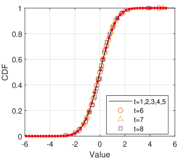
(a) Normalized samples of the real part of $\Delta_{t}(k)$.

(b) Normalized samples of the imaginary part of $\Delta_{t}(k)$.

Figure 2: Simulated CDF of $\Delta_{t}(k)$, $t=1,\dots,8$, ${\color[rgb]{0,0,0}k=256}$, with normalized samples. SNR=$0$ and $20$dB lead to similar results. The dots depict the CDF of $\mathcal{N}(0,1)$ as a reference.

VI-B Covariance of Frequency-Domain RCN

This simulation examines RCN property 3. We evaluate the normalized covariance of $\Delta_{t_{1}}(k)$ and $\Delta_{t_{2}}(k)$ for some sample values of $k$, defined as

$$\rho_{t_{1},t_{2}}{\color[rgb]{0,0,0}(k)}=\frac{\mathbb{E}\Big{\{}\big{(}\Delta_{t_{1}}(k)-\mathbb{E}\{\Delta_{t_{1}}(k)\}\big{)}\big{(}\Delta_{t_{2}}^{*}(k)-\mathbb{E}\{\Delta_{t_{2}}^{*}(k)\}\big{)}\Big{\}}}{\sqrt{\mathbb{V}[\Delta_{t_{1}}(k)]\mathbb{V}[\Delta_{t_{2}}(k)]}}.$$ (29)

Fig. 3 shows the result for $\gamma_{\text{eff}}=0$dB. It can be seen that ${\color[rgb]{0,0,0}|\rho_{t_{1},t_{2}}(k)|}=1$ for $t_{1}=t_{2}$ and ${\color[rgb]{0,0,0}|\rho_{t_{1},t_{2}}(k)|}\approx 0$ otherwise. The same result was observed for $\gamma_{\text{eff}}=10$, $20$, and $30$dB, and for randomly selected values of $k$. Since $\Delta_{t}(k)$ has zero mean (cf. property 2 and Fig. 2), this implies that $\mathbb{E}\{\Delta_{t_{1}}(k)\Delta_{t_{2}}^{*}(k)\}\approx 0$, and supports property 3.

Figure 3: Correlation coefficient between frequency-domain RCN from different layers for $k=256$.

VI-C RCN Power Estimation in an AWGN Channel

We examine the performance of the worst-case RCN power model in (11). Since the accuracy of the model depends on $\mathsf{f}(\cdot,\cdot,\cdot)$ which is approximated by considering a specific number of rims in the QAM constellation as discussed in Appendix B, we evaluate performance under different numbers of rims.

Fig. 4a compares the simulated and the estimated RCN power from layer 1 $\mathcal{P}\{{\bm{\delta}}_{1}\}$ using (11), under a flat AWGN channel, where $\mathcal{P}\{E_{t}(k)\}$ is estimated using (14) with $1$, $2$, or $3$ rims. When only one rim is considered, $p_{b},p_{c}$ in (31) should be set to $0$, and when only two rims are considered, $p_{c}$ in (31) should be set to $0$. The figure shows that the estimated RCN power is more accurate when more rims are considered at low effective SNR, and is accurate at moderate/high effective SNR for any number of rims. Moreover, $3$ rims are shown to be enough to obtain a good estimation in the whole tested range of $\gamma_{\text{eff}}$. It can also be seen that using the power of detection error $\mathcal{P}\{\mathbf{e}_{1}\}$ to approximate RCN power $\mathcal{P}\{{\bm{\delta}}_{1}\}$ (as suggested in [16, (13)]) results in an overestimation of RCN power.

Fig. 4b compares simulated and estimated $\mathcal{P}\{{\bm{\delta}}_{t}\}$, $t=1,\dots,8$ using 3 rims under a flat AWGN channel with $\gamma_{\text{eff}}=0$, $10$dB, and $20$dB, respectively. It can be seen that the estimated $\mathcal{P}\{{\bm{\delta}}_{t}\}$ closely follows the simulation results. The estimation performance is generally better when $\gamma_{\text{eff}}$ is moderate/large. When $\gamma_{\text{eff}}$ is small, accurate estimation of detection-error power $\mathcal{P}\{E_{t}(k)\}$ requires more than 3 rims. Similarly, in high layers such as layers $6,7,8$, RCN is accumulated leading to stronger noise, and thus more rims are also required for accurate estimation of $\mathcal{P}\{E_{t}(k)\}$. This leads to an underestimation of RCN power in some cases. Another reason for the underestimation of RCN power in high layers is the model mismatch when the number of effective subcarriers is small.

(a) RCN power from layer 1 versus $\gamma_{\text{eff}}$.

(b) RCN power from all layers.

Figure 4: Comparison of simulated and estimated RCN power a flat AWGN channel.

We also run a similar simulation in a frequency-selective channel with channel-inversion equalization at the receiver. The channel gain of the tested frequency-selective channel is the one shown in [1, Fig. 4b] converted to our $1024$-subcarrier LACO-OFDM system. Simulation results are given in Fig. 5, which shows similar trends as in Fig. 4, i.e., the estimated RCN power is close to the simulated value for each layer under each $\gamma_{\text{eff}}$.

(a) RCN power from layer 1 versus $\gamma_{\text{eff}}$.

(b) RCN power from all layers.

Figure 5: Comparison of simulated and estimated RCN power in a frequency-selective AWGN channel.

VI-D SER Evaluation

In this simulation, the SER for ADO-OFDM, HACO-OFDM and LACO-OFDM discussed in Sec. IV is examined. For a fair comparison, all schemes are tested under the same electrical power $P_{\text{elec}}$ and a modulation order of $16$, i.e., $M_{t}(k)=16$, $\forall t,k\in\mathcal{B}_{t}$. Each scheme equally distributes its effective power $P_{\text{eff}}$ in all effective subcarriers, where $P_{\text{eff}}$ is obtained from $P_{\text{elec}}$ using Table I.

Fig. 6a compares the simulated SER with evaluated SER using an RCN-aware and an RCN-unaware model, in a flat AWGN channel. In the RCN-aware evaluation, the total noise power is evaluated using (18), otherwise the total noise power is $\mathcal{P}\{V(k)\}$. It can be seen the RCN-aware SER evaluation always matches the simulation results, while the RCN-unaware SER evaluation does not for most of the SNR in LACO-OFDM and ADO-OFDM. The figure shows that HACO-OFDM has the best tolerance to RCN among the three schemes, as the RCN-unaware SER is close to the simulation result. This is because PAM-DMT subcarriers only use imaginary symbols and thus are not affected by the the real part of RCN. Similar results can be seen in Fig. 6b which compares the SER in the frequency-selective AWGN channel in [1, Fig. 4b] with channel-inversion equalization at the receiver. Again, the RCN-aware SER evaluation closely matches the simulation results.

(a) Flat AWGN channel.

(b) Frequency-selective AWGN channel.

Figure 6: Simulated and evaluated SER comparison for ADO-OFDM, HACO-OFDM and LACO-OFDM in an AWGN channel, where $16$-QAM (or $16$-PAM for the PAM-DMT layer of HACO-OFDM) is used in all subcarriers. The filled (empty) circle, triangle, and square markers represent the theoretical RCN-aware (RCN-unaware) SER evaluation of ADO-OFDM, HACO-OFDM and LACO-OFDM, respectively.

Note that a similar trend as in Fig. 6 has been observed for smaller $N$, such as $N=64$ instead of $1024$, which indicates that the model is relevant even at relatively small $N$.

VI-E SER-controlled LACO-OFDM

Here, we examine the SER-controlled LACO-OFDM scheme proposed in Sec. V under the frequency-selective channel in [1, Fig. 4b]. We use (28) to obtain the theoretical SER performance of the proposed resource allocation scheme. The theoretical SER are compared to simulated SER to show the accuracy of the proposed SER calculation. For resource allocation, the SER target is set at $p_{\rm e}=10^{-2}$ (as an example) which leads to a BER in the order of $10^{-3}$. The convergence criterion is set $\epsilon=10^{-3}\frac{\|{\bf{P}}_{z}^{i}\|^{2}}{N}$.

Fig. 7a compares the theoretical and simulation SER performance of the resource allocation scheme. Both RCN-aware and RCN-unaware resource allocation are considered, where RCN-unaware resource allocation is realized by using $P_{z}^{(i+1)}=\mathcal{P}\{V(k)\}$ in the resource allocation algorithm instead of $P_{z}^{(i+1)}=\mathcal{P}\{V(k)\}+\sum_{t=1}^{j_{k}-1}P_{t}^{\rm w}$. It can be seen that most theoretical and simulated SER values match for most $P_{\rm eff}$. Mismatch happens when the average number of bits per subcarrier is 1 or 3, i.e., when 2QAM and 8QAM are used, which makes (19) inaccurate [26]. It can also be seen that RCN-aware resource allocation controls the SER perfectly under the $10^{-2}$ constraint for almost all $\gamma_{\text{eff}}$, which guarantees the SER performance. For gray-coding at high $\gamma_{\text{eff}}$, BER can be evaluated from SER through the relation $\text{BER}\approx\frac{\text{SER}}{\bar{n}_{b}}$, where $\bar{n}_{b}$ is the average number of bits per subcarrier among all the layers. Take the $15-30$dB $\gamma_{\text{eff}}$ region as an example. In this region, the average number of bits per subcarrier is from 3 to 8, thus the BER is in the range from $1.25\times 10^{-3}$ to $3.33\times 10^{-3}$. When the BER range is known, coding schemes can be chosen to provide guaranteed coding gain [28, 29], and leading to a more predictable coding performance (BER after decoding). Therefore, the proposed RCN power model and the proposed SER-controlled LACO-OFDM resource allocation scheme can guarantee reliable system performance. Fig. 7a also shows that 2 iterations of the resource allocation algorithm lead to an SER which is almost the same as the SER after convergence.

Fig. 7b shows the average number of bits per subcarrier allocated under each $\gamma_{\text{eff}}$. The figure shows that the RCN-aware scheme is more conservative in allocating bits than the RCN-unaware scheme, since it takes RCN into account. This is reflected as higher reliability in Fig. 7a since the target SER is more likely to be met than when RCN-unaware allocation is used.

(a) SER versus effective SNR.

(b) Averaged number of allocated bits per subcarrier.

Figure 7: Performance of SER-controlled LACO-OFDM under a $10^{-2}$ target SER constraint. The dotted line and the dashed line are almost overlapping.

VII Conclusion

In this paper, we studied residual clipping noise in several enhanced ACO-OFDM schemes, including ADO-OFDM, HACO-OFDM, and LACO-OFDM. We proposed a worst-case RCN power model, which provides an accurate evaluation of total noise power and symbol error rate, and is the first accurate RCN power model in the literature. Using the proposed RCN power model, we have proposed an RCN-aware resource allocation algorithm for enhanced ACO-OFDM, which is reliable in terms of achieving a target SER performance. The proposed model can be used in general system analysis and optimization research in enhanced ACO-OFDM, such as bit loading, power allocation, data rate maximization, error rate minimization, etc., and is hence of practical significance.

It is worthwhile to note that, as future work, it would be interesting to extend this model to systems with a peak intensity constraint, where peak-clipping distortion should be accounted for. Moreover, it is interesting to study the trade-off between complexity and error-rate performance when the RCN-aware design is combined with channel coding, which will shed light on the design of practical eACO-OFDM systems.

Appendix A Derivation of Power Relations

This section proves the power relations listed in Table I. We first recall Lemma 1 in Sec. III-B which will be used in what follows. Lemma 1 states that if the number of loaded subcarriers in $S(k)$ is large, and $S(k)$ is zero-mean and bounded for all $k$ and Hermitian symmetric, then $s(n)$ converges in distribution for all $n$ to a Gaussian distribution $\mathcal{N}(0,\sigma^{2})$ for some $\sigma^{2}$. Consequently, clipping out negative $s(n)$ generates $x(n)=(s(n))^{+}=\frac{s(n)+|s(n)|}{2}$ whose distribution (for all $n$) is $\mathcal{N}_{c}\big{(}0,\sigma^{2},[0,\infty)\big{)}$ defined by the probability density function

$$p_{X}(x)=\begin{cases}\frac{1}{\sqrt{2\pi}\sigma}{e^{-\frac{x^{2}}{2\sigma^{2}}}}&x>0,\\ \frac{1}{2}\sdelta(x)&x=0,\end{cases}$$ (30)

with mean $\mathbb{E}\{x(n)\}=\frac{\sigma}{\sqrt{2\pi}}$ and second moment $\mathbb{E}\{x^{2}(n)\}=\frac{\sigma^{2}}{2}$, where $\sdelta(x)$ is the Dirac impulse.

An ACO-OFDM signal is given by $x_{\rm aco}(n)=(s_{\rm aco}(n))^{+}$. By Lemma 1, $s_{\rm aco}(n)\sim\mathcal{N}(0,\sigma^{2})$ for some $\sigma^{2}$. Hence, $x_{\rm aco}(n)\sim\mathcal{N}_{c}\big{(}0,\sigma^{2},[0,\infty)\big{)}$ for all $n$. Thus, $P_{\text{elec}}=\frac{1}{N}\sum_{n=0}^{N-1}\mathbb{E}[x_{\rm aco}^{2}(n)]$ by the law of large numbers, leading to $P_{\text{elec}}=\frac{\sigma^{2}}{2}$. Similarly, we can write $P_{\text{opt}}=\frac{1}{N}\sum_{n=0}^{N-1}\mathbb{E}[x_{\rm aco}(n)]=\frac{\sigma}{\sqrt{2\pi}}$. We also have $P_{\text{eff}}=\mathcal{P}\{\frac{\mathbf{s}_{\rm aco}}{2}\}=\frac{1}{N}\sum_{n=0}^{N-1}\mathbb{E}[(\frac{s_{\rm aco}(n)}{2})^{2}]=\frac{\sigma^{2}}{4}$. Therefore, we have that $P_{\text{elec}}=2P_{\rm eff}$ and $P_{\text{opt}}=\sqrt{\frac{2P_{\rm eff}}{\pi}}$ as stated in Table I.

For DCO-OFDM, the signal $x_{\rm dco}(n)$ is given by $x_{\rm dco}(n)=(s_{\rm dco}(n)+d_{\rm dco})^{+}$. Recall that $s_{\rm dco}(n)\sim\mathcal{N}(0,\sigma^{2})$ for some $\sigma^{2}$ by Lemma 1. By choosing $d_{\rm dco}=3\sigma$, we can approximate $x_{\rm dco}(n)\approx s_{\rm dco}(n)+d_{\rm dco}$. Hence, we can approximate $x_{\rm dco}(n)$ to be $\mathcal{N}(d_{\rm dco},\sigma^{2})$. Then, we have $P_{\text{elec}}=\frac{1}{N}\sum_{n=0}^{N-1}\mathbb{E}[x_{\rm dco}^{2}(n)]=10\sigma^{2}$ and $P_{\text{opt}}=\frac{1}{N}\sum_{n=0}^{N-1}\mathbb{E}[x_{\rm dco}(n)]=3\sigma$. We also have $P_{\text{eff}}=\mathcal{P}\{\mathbf{s}_{\rm dco}\}=\sigma^{2}$. We conclude that $P_{\text{elec}}=10P_{\rm eff}$ and $P_{\text{opt}}=3\sqrt{P_{\rm eff}}$ as shown in Table I.

The analysis of PAM-DMT omitted since it is similar to that of ACO-OFDM, leading to the relations $P_{\text{elec}}=2P_{\rm eff}$ and $P_{\text{opt}}=\sqrt{\frac{2P_{\rm eff}}{\pi}}$ as stated in Table I.

For an ADO-OFDM, the transmit signal is $x_{\rm ado}(n)=x_{1}(n)+x_{2}(n)$, where $x_{1}(n)=(s_{\rm aco}(n))^{+}$ is the ACO-OFDM signal in layer 1, $x_{2}(n)=(s_{\rm dco}^{(2)}(n)+d_{\rm dco}^{(2)})^{+}$ is the DCO-OFDM signal in layer 2. Note that $s_{\rm aco}(n)\sim\mathcal{N}(0,\sigma_{1}^{2})$ and $s_{\rm dco}^{(2)}(n)\sim\mathcal{N}(0,\sigma_{2}^{2})$ for some $\sigma_{1}^{2}$ and $\sigma^{2}_{2}$ by Lemma 1. Then $x_{1}(n)\sim\mathcal{N}_{c}\big{(}0,\sigma_{1}^{2},[0,\infty)\big{)}$. Moreover, by choosing $d_{\rm dco}^{(2)}=3\sigma_{2}$, $x_{2}(n)\sim\mathcal{N}(3\sigma_{2},\sigma_{2}^{2})$. Thus, using the law of large numbers, we have $P_{\text{elec}}=\frac{1}{N}\sum_{n=0}^{N-1}\mathbb{E}[x_{\rm ado}^{2}(n)]=\frac{1}{N}\sum_{n=0}^{N-1}\mathbb{E}[(x_{1}(n)+x_{2}(n))^{2}]=\frac{\sigma_{1}^{2}}{2}+10\sigma_{2}^{2}+\frac{6}{\sqrt{2\pi}}\sigma_{1}\sigma_{2}$ and $P_{\text{opt}}=\frac{1}{N}\sum_{n=0}^{N-1}\mathbb{E}[x_{\rm ado}(n)]=\frac{1}{N}\sum_{n=0}^{N-1}\mathbb{E}[x_{1}(n)+x_{2}(n)]=\frac{\sigma_{1}}{\sqrt{2\pi}}+3\sigma_{2}$. We also have $P_{\text{eff}}=\mathcal{P}\{\frac{\mathbf{s}_{\rm aco}}{2}+\mathbf{s}_{\rm dco}^{(2)}\}=\frac{\sigma_{1}^{2}}{4}+\sigma_{2}^{2}$. Letting $\sigma_{2}=\alpha\sigma_{1}$ for some $\alpha$, then $P_{\text{elec}}$, $P_{\text{opt}}$, and $P_{\text{eff}}$ can be related through $\sigma_{1}$ for a general $\alpha$. By setting $\alpha=\frac{1}{2}$ which equally distributes $P_{\text{eff}}$ in all effective subcarriers of ADO-OFDM, we obtain $P_{\rm elec}=(6+\frac{6}{\sqrt{2\pi}})P_{\rm eff}$ and $P_{\rm opt}=(\frac{1}{\sqrt{\pi}}+\frac{3}{\sqrt{2}})\sqrt{P_{\rm eff}}$ as shown in Table I.

In HACO-OFDM, the transmit signal is $x_{\rm haco}(n)=x_{1}(n)+x_{2}(n)$, where $x_{1}(n)=(s_{\rm aco}(n))^{+}$ is the ACO-OFDM signal in layer 1 and $x_{2}(n)=(s_{\rm pam}(n))^{+}$ is the PAM-DMT signal in layer 2. Using Lemma 1, we have that $s_{\rm aco}(n)\sim\mathcal{N}(0,\sigma_{1}^{2})$ and $s_{\rm pam}(n)\sim\mathcal{N}(0,\sigma_{2}^{2})$ for some $\sigma_{1}^{2}$ and $\sigma_{2}^{2}$. Therefore, $x_{i}(n)\sim\mathcal{N}_{c}\big{(}0,\sigma_{i}^{2},[0,\infty)\big{)}$. Then, using the law of large numbers, we have $P_{\text{elec}}=\frac{1}{N}\sum_{n=0}^{N-1}\mathbb{E}[x_{\rm haco}^{2}(n)]=\mathbb{E}[(x_{1}(n)+x_{2}(n))^{2}]=\frac{\sigma_{1}^{2}+\sigma_{2}^{2}}{2}+\frac{\sigma_{1}\sigma_{2}}{\pi}$ and $P_{\text{opt}}=\frac{1}{N}\sum_{n=0}^{N-1}\mathbb{E}[x_{\rm haco}(n)]=\mathbb{E}[x_{1}(n)+x_{2}(n)]=\frac{\sigma_{1}+\sigma_{2}}{\sqrt{2\pi}}$. We also have $P_{\text{eff}}=\mathcal{P}\{\frac{\mathbf{s}_{\rm aco}}{2}+\frac{\mathbf{s}_{\rm pam}}{2}\}=\frac{\sigma_{1}^{2}+\sigma_{2}^{2}}{4}$. In general, letting $\sigma_{2}=\alpha\sigma_{1}$ for some $\alpha$, we can obtain relations among $P_{\rm elec}$, $P_{\rm opt}$ and $P_{\rm eff}$ through $\sigma_{1}$. By setting $\alpha=1$ which equally distributes $P_{\text{eff}}$ in all effective subcarriers of HACO-OFDM, we obtain $P_{\rm elec}=(2+\frac{2}{\pi})P_{\rm eff}$ and $P_{\rm opt}=\frac{2}{\sqrt{\pi}}\sqrt{P_{\rm eff}}$ as shown in Table I.

For LACO-OFDM, the transmit signal is $x_{\rm laco}(n)=\sum_{i=1}^{J}x_{i}(n)$, where $x_{i}(n)=(s_{\rm aco}^{(i)}(n))^{+}$ is the ACO-OFDM signal in layer $i$. Using Lemma 1, we have that $s_{\rm aco}^{(i)}(n)\sim\mathcal{N}(0,\sigma_{i}^{2})$ for some $\sigma_{i}^{2}$. Therefore, $x_{i}(n)\sim\mathcal{N}_{c}\big{(}0,\sigma_{i}^{2},[0,\infty)\big{)}$. Then, using the law of large numbers, we have $P_{\text{elec}}=\frac{1}{N}\sum_{n=0}^{N-1}\mathbb{E}[x_{\rm laco}^{2}(n)]=\frac{1}{N}\sum_{n=0}^{N-1}\mathbb{E}[(\sum_{i=1}^{J}x_{i}(n))^{2}]=\sum_{i=1}^{J}(\frac{1}{2}-\frac{1}{2\pi})\sigma_{i}^{2}+(\sum_{i}\frac{\sigma_{i}}{\sqrt{2\pi}})^{2}$ and $P_{\text{opt}}=\frac{1}{N}\sum_{n=0}^{N-1}\mathbb{E}[x_{\rm laco}(n)]=\frac{1}{N}\sum_{n=0}^{N-1}\mathbb{E}[\sum_{i=1}^{J}x_{i}(n)]=\sum_{i}\frac{\sigma_{i}}{\sqrt{2\pi}}$. We also have $P_{\text{eff}}=\mathcal{P}\{\sum_{i=1}^{J}\frac{\mathbf{s}_{\rm aco}^{(i)}}{2}\}=\frac{\sum_{i=1}^{J}\sigma_{i}^{2}}{4}$. Let $\sigma_{i}^{2}=\alpha_{i}\sigma^{2}$ for some $\alpha_{i}$ and $\sigma^{2}$. Then a relation between $P_{\text{elec}}$, $P_{\text{opt}}$, and $P_{\text{eff}}$ can be readily obtained through $\sigma^{2}$. By choosing $\alpha_{i}=2^{J-i}$ for $i\in\{1,\ldots,J\}$, which means that $P_{\rm eff}$ is equally distributed in all effective subcarriers, then we obtain $P_{\text{elec}}=(2-\frac{2}{\pi}+\frac{2}{(3-2\sqrt{2})\pi}\frac{\sqrt{2}^{J}-1}{\sqrt{2}^{J}+1})P_{\text{eff}}$ and $P_{\text{opt}}=\sqrt{\frac{2}{(3-2\sqrt{2})\pi}\frac{\sqrt{2}^{J}-1}{\sqrt{2}^{J}+1}P_{\text{eff}}}$ as shown in Table I.

Appendix B Approximation of Detection-Error Power for QAM Constellations

Consider an $M$-QAM symbol $x$ that is transmitted over a flat AWGN channel, and received at the receiver as $y=x+n$ where $n$ is $\mathcal{CN}(0,\sigma^{2})$. The receiver adopts an ML detector to detect $\hat{x}$. Let the position of $x$ in the constellation be position $0$ as shown in Fig. 8. Noise will confuse the ML detector between the transmitted symbol and its neighbors, and an error will take place when $y$ falls outside position 0.

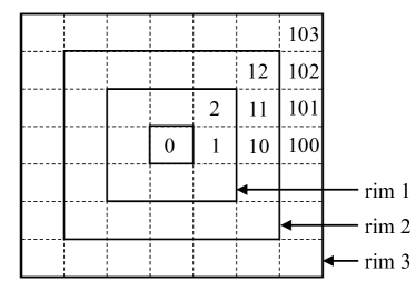
Figure 8: Geometry of 3 rims.

We focus on neighbors of the transmitted symbol within the first three rims of position 0 and assume that the probability of $y$ falling outside the first three rims is negligible. We index the positions in the three rims using one-digit numbers starting from 1, two-digit numbers starting from 10, and three-digit numbers starting from 100, respectively. We also denote the Euclidean distance between position 0 and position $i$ by $d_{i}$, the minimum Euclidean distance of the used $M$-QAM constellation by $d_{\text{min}}$, and the error probability of detecting a symbol $\hat{x}$ at position $i$ by $p_{i}$ (i.e., the probability that $y$ falls in position $i$).

Note that an error event in a QAM constellation can be considered as two independent error events in a PAM constellation where the noise is the real part or the imaginary part of $n$ [26]. Denote the real part of $n$ by $n_{\rm r}$, and let $p_{a}$, $p_{b}$, and $p_{c}$ be the probabilities that $n_{\rm r}$ is larger than $\frac{d_{\rm min}}{2}$, $\frac{3d_{\rm min}}{2}$, and $\frac{5d_{\rm min}}{2}$, respectively, i.e.,

$$p_{a}=\mathsf{Q}\left(\frac{d_{\text{min}}}{\sqrt{2}\sigma}\right),\;\;p_{b}=\mathsf{Q}\left(\frac{3d_{\text{min}}}{\sqrt{2}\sigma}\right),\;\;p_{c}=\mathsf{Q}\left(\frac{5d_{\text{min}}}{\sqrt{2}\sigma}\right).$$ (31)

Then, for the first three rims in a QAM constellation, we have

$$p_{1} =(p_{a}-p_{b})(1-2p_{a}),\;\;\;p_{2}=(p_{a}-p_{b})^{2};$$ (32)

$$p_{10} =(p_{b}-p_{c})(1-2p_{a}),\;\;p_{11}=(p_{b}-p_{c})(p_{a}-p_{b}),\;\;p_{12}=(p_{b}-p_{c})^{2};$$ (33)

$$p_{101} =p_{c}(p_{a}-p_{b}),\;\;\quad\quad\;\;p_{102}=p_{c}(p_{b}-p_{c}),\;\;\quad\quad\;\;p_{103}=p_{c}^{2}.$$ (34)

For the first three rims of position 0, the power of detection error can be expressed as

$$P_{0}={\color[rgb]{0,0,0}\mathbb{E}\{|x-\hat{x}|^{2}\}=}\sum_{i\in\mathcal{A}}{d_{i}^{2}p_{i}n_{i}},$$ (35)

where $\mathcal{A}=\{1,\;2,\;10,\;11,\;12,\;100,\;101,\;102,\;103\}$ and $n_{i}$ is the number of neighboring points at a distance $d_{i}$ from $x$.

The former discussion applies when $x$ is in position $0$. To estimate the power of detection errors when all points of the $M$-QAM constellation are considered, we assume that all points in the constellation are transmitted with the same probability. In this case, $n_{i}$ in (35) should be replaced with the average number of neighbors at a distance $d_{i}$ from $x$, which is denoted by $\bar{n}_{i}^{M-\text{QAM}}$. Then the power of detection errors for a $M$-QAM constellation, $P_{\rm e}^{M-\text{QAM}}$, can be obtained by modifying (35) to

$$P_{\rm e}^{M-\text{QAM}}=\sum_{i\in\mathcal{A}}{d_{i}^{2}p_{i}\bar{n}_{i}^{M-\text{QAM}}}.$$ (36)

The calculation of (36) only requires the minimum Euclidean distance $d_{\text{min}}$, noise power $\sigma^{2}$ and constellation size $M$. Therefore we can write

$$P_{\rm e}^{M-\text{QAM}}={\color[rgb]{0,0,0}\mathsf{f}}(d_{\text{min}},{\color[rgb]{0,0,0}\sigma^{2}},M),$$ (37)

as given in Definition 1.

References

- [1] Z. Zhang, A. Chaaban, C. Shen, H. Elgala, T. K. Ng, B. S. Ooi, and M.-S. Alouini, “Worst-case residual clipping noise power model for bit loading in LACO-OFDM,” in 2018 Global LIFI Congress (GLC). IEEE, 2018, pp. 1–6.
- [2] H. Burchardt, N. Serafimovski, D. Tsonev, S. Videv, and H. Haas, “VLC: Beyond point-to-point communication,” IEEE Communications Magazine, vol. 52, no. 7, pp. 98–105, 2014.
- [3] L. Hanzo, H. Haas, S. Imre, D. O’Brien, M. Rupp, and L. Gyongyosi, “Wireless myths, realities, and futures: from 3G/4G to optical and quantum wireless,” Proceedings of the IEEE, vol. 100, no. Special Centennial Issue, pp. 1853–1888, 2012.
- [4] A. Chaaban, Z. Rezki, and M.-S. Alouini, “On the capacity of the intensity-modulation direct-detection optical broadcast channel,” IEEE Transactions on Wireless Communications, vol. 15, no. 5, pp. 3114–3130, 2016.
- [5] Z. Ghassemlooy, W. Popoola, and S. Rajbhandari, Optical wireless communications: system and channel modelling with Matlab®. CRC press, 2019.
- [6] D. J. Barros, S. K. Wilson, and J. M. Kahn, “Comparison of orthogonal frequency-division multiplexing and pulse-amplitude modulation in indoor optical wireless links,” IEEE Transactions on Communications, vol. 60, no. 1, pp. 153–163, 2011.
- [7] J. Armstrong, B. J. Schmidt, D. Kalra, H. A. Suraweera, and A. J. Lowery, “SPC07-4: Performance of asymmetrically clipped optical OFDM in AWGN for an intensity modulated direct detection system,” in IEEE Globecom 2006. IEEE, 2006, pp. 1–5.
- [8] S. C. J. Lee, S. Randel, F. Breyer, and A. M. Koonen, “PAM-DMT for intensity-modulated and direct-detection optical communication systems,” IEEE Photonics Technology Letters, vol. 21, no. 23, pp. 1749–1751, 2009.
- [9] M. S. Islim, D. Tsonev, and H. Haas, “Spectrally enhanced PAM-DMT for IM/DD optical wireless communications,” in 2015 IEEE 26th annual international symposium on personal, indoor, and mobile radio communications (PIMRC). IEEE, 2015, pp. 877–882.
- [10] J. Zhou, Q. Wang, Q. Cheng, M. Guo, Y. Lu, A. Yang, and Y. Qiao, “Low-papr layered/enhanced ACO-SCFDM for optical-wireless communications,” IEEE Photonics Technology Letters, vol. 30, no. 2, pp. 165–168, 2017.
- [11] S. D. Dissanayake and J. Armstrong, “Comparison of ACO-OFDM, DCO-OFDM and ADO-OFDM in IM/DD systems,” Journal of lightwave technology, vol. 31, no. 7, pp. 1063–1072, 2013.
- [12] B. Ranjha and M. Kavehrad, “Hybrid asymmetrically clipped OFDM-based IM/DD optical wireless system,” Journal of Optical Communications and Networking, vol. 6, no. 4, pp. 387–396, 2014.
- [13] Q. Wang, C. Qian, X. Guo, Z. Wang, D. G. Cunningham, and I. H. White, “Layered ACO-OFDM for intensity-modulated direct-detection optical wireless transmission,” Optics Express, vol. 23, no. 9, pp. 12 382–12 393, 2015.
- [14] E. Lam, S. K. Wilson, H. Elgala, and T. D. Little, “Spectrally and energy efficient OFDM (SEE-OFDM) for intensity modulated optical wireless systems,” arXiv preprint arXiv:1510.08172, 2015.
- [15] B. Li, W. Xu, H. Zhang, C. Zhao, and L. Hanzo, “PAPR reduction for hybrid ACO-OFDM aided IM/DD optical wireless vehicular communications,” IEEE Transactions on Vehicular Technology, vol. 66, no. 10, pp. 9561–9566, 2017.
- [16] X. Zhang, Q. Wang, R. Zhang, S. Chen, and L. Hanzo, “Performance analysis of layered ACO-OFDM,” IEEE Access, vol. 5, pp. 18 366–18 381, 2017.
- [17] T. Q. Wang, H. Li, and X. Huang, “Analysis and mitigation of clipping noise in layered ACO-OFDM based visible light communication systems,” IEEE Transactions on Communications, vol. 67, no. 1, pp. 564–577, 2018.
- [18] A. J. Lowery, “Comparisons of spectrally-enhanced asymmetrically-clipped optical ofdm systems,” Optics express, vol. 24, no. 4, pp. 3950–3966, 2016.
- [19] Y. Sun, F. Yang, and J. Gao, “Comparison of hybrid optical modulation schemes for visible light communication,” IEEE Photonics Journal, vol. 9, no. 3, pp. 1–13, 2017.
- [20] A. J. Lowery, “Comparisons of spectrally-enhanced asymmetrically-clipped optical ofdm systems,” Optics express, vol. 24, no. 4, pp. 3950–3966, 2016.
- [21] J. Zhou and W. Zhang, “A comparative study of unipolar OFDM schemes in gaussian optical intensity channel,” IEEE Transactions on Communications, vol. 66, no. 4, pp. 1549–1564, 2017.
- [22] X. Zhang, Z. Babar, R. Zhang, S. Chen, and L. Hanzo, “Multi-class coded layered asymmetrically clipped optical OFDM,” IEEE Transactions on Communications, vol. 67, no. 1, pp. 578–589, 2018.
- [23] J. Campello, “Practical bit loading for DMT,” in 1999 IEEE International Conference on Communications (Cat. No. 99CH36311), vol. 2. IEEE, 1999, pp. 801–805.
- [24] A. M. Wyglinski, F. Labeau, and P. Kabal, “Bit loading with BER-constraint for multicarrier systems,” IEEE Transactions on wireless communications, vol. 4, no. 4, pp. 1383–1387, 2005.
- [25] Y. Sun, F. Yang, and J. Gao, “Near-optimal power allocation and layer assignment for laco-ofdm in visible light communication,” in GLOBECOM 2017-2017 IEEE Global Communications Conference. IEEE, 2017, pp. 1–6.
- [26] J. G. Proakis and M. Salehi, “Optimum receivers for AWGN channels,” Digital Communications, vol. 5, 2008.
- [27] P. Billingsley, “The central limit theorem,” in Probability and Measure. John Wiley and Sons, 2008.
- [28] J. M. Cioffi, G. P. Dudevoir, M. V. Eyuboglu, and G. D. Forney, “MMSE decision-feedback equalizers and coding. II. coding results,” IEEE Transactions on Communications, vol. 43, no. 10, pp. 2595–2604, 1995.
- [29] ITU-T, “G.975.1: Forward error correction for high bit-rate DWDM submarine systems,” in Transmission Systems and Media, Digital Systems and Networks, Geneva, Switzerland, 2004.