On the uncertainty of self-supervised monocular depth estimation

Abstract

Self-supervised paradigms for monocular depth estimation are very appealing since they do not require ground truth annotations at all. Despite the astonishing results yielded by such methodologies, learning to reason about the uncertainty of the estimated depth maps is of paramount importance for practical applications, yet uncharted in the literature. Purposely, we explore for the first time how to estimate the uncertainty for this task and how this affects depth accuracy, proposing a novel peculiar technique specifically designed for self-supervised approaches. On the standard KITTI dataset, we exhaustively assess the performance of each method with different self-supervised paradigms. Such evaluation highlights that our proposal i) always improves depth accuracy significantly and ii) yields state-of-the-art results concerning uncertainty estimation when training on sequences and competitive results uniquely deploying stereo pairs.

1 Introduction

Depth estimation is often pivotal to a variety of high-level tasks in computer vision, such as autonomous driving, augmented reality, and more. Although active sensors such as LiDAR are deployed for some of the applications mentioned above, estimating depth from standard cameras is generally preferable due to several advantages. Among them: the much lower cost of standard imaging devices, their higher resolution and frame rate allow for more scalable and compelling solutions.

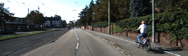
\begin{overpic}[width=198.73946pt]{plots/magma.png} \put(1.0,1.0){$\displaystyle{\color[rgb]{0,1,0}\text{Far}}$} \put(90.0,1.0){$\displaystyle{\color[rgb]{1,0,0}\text{Close}}$} \end{overpic}

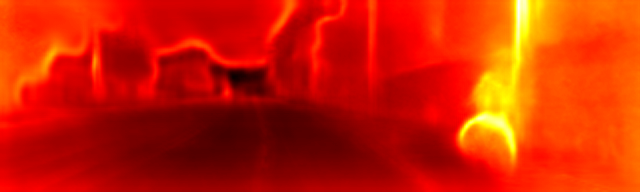
\begin{overpic}[width=198.73946pt]{plots/hot.png} \put(1.0,1.0){$\displaystyle{\color[rgb]{0,1,0}\text{Low}}$} \put(90.0,1.0){$\displaystyle{\color[rgb]{1,0,0}\text{High}}$} \end{overpic}

Figure 1: How much can we trust self-supervised monocular depth estimation? From a single input image (top) we estimate depth (middle) and uncertainty (bottom) maps. Best with colors.

In computer vision, depth perception from two [59] or multiple images [60] has a long history. Nonetheless, only in the last decade depth estimation from a single image [57] became an active research topic. On the one hand, this direction is particularly attractive because it overcomes several limitations of the traditional multi-view solutions (e.g., occlusions, overlapping framed area, and more), enabling depth perception with any device equipped with a camera. Unfortunately, it is an extremely challenging task due to the ill-posed nature of the problem.

Deep learning ignited the spread of depth-from-mono frameworks [13, 38, 15], at the cost of requiring a large number of image samples annotated with ground truth depth labels [47, 68] to achieve satisfying results. However, sourcing annotated depth data is particularly expensive and cumbersome. Indeed, in contrast to many other supervised tasks for which offline handmade annotation is tedious, yet relatively easy, gathering accurate depth labels requires active (and often expensive) sensors and specific calibration, making offline annotation hardly achievable otherwise. Self-supervised [19, 82, 45, 56, 53] or weakly supervised [76, 65, 72] paradigms, leveraging on image reprojection and noisy labels respectively, have removed this issue and yield accuracy close to supervised methods [15], neglecting at all the deployment of additional depth sensors for labeling purposes. Among self-supervised paradigms, those deploying monocular sequences are more challenging since scale and camera poses are unknown, yet preferred for most practical applications since they allow gathering of training data with the same device used to infer depth.

As for other perception strategies, it is essential to find out failure cases, when occurring, in monocular depth estimation networks. For instance, in an autonomous driving scenario, the erroneous perception of the distance to pedestrians or other vehicles might have dramatic consequences. Moreover, the ill-posed nature of depth-from-mono perception task makes this eventuality much more likely to occur compared to techniques leveraging scene geometry [59, 60]. In these latter cases, estimating the uncertainty (or, complementary, the confidence) proved to be effective for depth-from-stereo, by means of both model-based [24] and learning-based [55, 30] methods, optical flow [27], and semantic segmentation [26, 30]. Despite the steady progress in other related fields, uncertainty estimation for self-supervised paradigms remains almost unexplored or, when faced, not quantitatively evaluated [32].

Whereas concurrent works in this field [20, 72, 65] targeted uniquely depth accuracy, we take a breath on this rush and focus for the first time, to the best of our knowledge, on uncertainty estimation for self-supervised monocular depth estimation networks, showing how this practise enables to improve depth accuracy as well.

Our main contributions can be summarized as follows:

• A comprehensive evaluation of uncertainty estimation approaches tailored for the considered task.

• An in-depth investigation of how the self-supervised training paradigm deployed impacts uncertainty and depth estimation.

• A new and peculiar Self-Teaching paradigm to model uncertainty, particularly useful when the pose is unknown during the training process, always enabling to improve depth accuracy.

Deploying standard metrics in this field, we provide exhaustive experimental results on the KITTI dataset [18]. Figure 1 shows the output of a state-of-the-art monocular depth estimator network enriched to model uncertainty. We can notice how our proposal effectively allows to detect wrong predictions (e.g., in the proximity of the person riding the bike).

2 Related work

In this section, we review the literature concerning self-supervised monocular depth estimation and techniques to estimate uncertainty in deep neural networks.

Self-supervision for mono. The advent of deep learning, together with the increasing availability of ground truth depth data, led to the development of frameworks [38, 40, 74, 15] achieving unpaired accuracy compared to previous approaches [58, 37, 14]. Nonetheless, the effort to collect large amounts of labeled images is high. Thus, to overcome the need for ground truth data, self-supervision in the form of image reconstruction represents a prevalent research topic right now. Frameworks leveraging on this paradigm belong to two (not mutually exclusive) categories, respectively supervised through monocular sequences or stereo pairs.

The first family of networks jointly learns to estimate the depth and relative pose between two images acquired by a moving camera. Seminal work in this direction is [82], extended by leveraging on point-cloud alignment [45], differentiable DVO [69], optical flow [78, 83, 11, 3], semantic [66] or scale consistency [5]. One of the shortcomings of these approaches is represented by moving objects appearing in the training images, addressed in [8, 75] employing instance segmentation and subsequent motion estimation of the segmented dynamic objects.

For the second category, pivotal are the works by Garg et al. [17] and Godard et al. [19]. Other methods improved efficiency [53, 50] to enable deployment on embedded devices, or accuracy by simulating a trinocular setup [56], jointly learning for semantic [79], using higher resolution [51], GANs [1], sparse inputs from visual odometry [2] or a teacher-student scheme [52]. Finally, approaches leveraging both kind of supervisions have been proposed in [80, 77, 41, 20].

Weak-supervision for mono. A trade-off between self and full supervision is represented by another family of approaches leveraging weaker annotations. In this case, labels can be sourced from synthetic datasets [46], used to train stereo networks for single view stereo [42] and label distillation [22] or in alternative to learn depth estimation and perform domain transfer when dealing with real images [4].

Another source of weak supervision consists of using noisy annotations obtained employing the raw output of a LiDAR sensor [35] or model-based algorithms. In this latter case, the use of conventional stereo algorithms such as SGM [23] to obtain proxy labels [65, 72], optionally together with confidence measures [64], allowed improving self-supervision from stereo pairs. Other works distilled noisy labels leveraging on structure from motion [32] or direct stereo odometry [76].

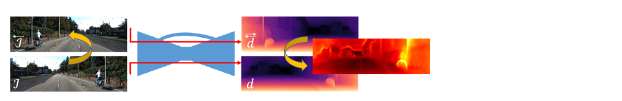
Figure 2: Overview of uncertainty estimation implementations. Respectively a) empirical methods model uncertainty as the variance of predictions from a subset of all the possible instances of the same network, b) predictive are trained to estimate depth and uncertainty as mean and variance of a distribution and c) Bayesian methods are approximated [48] by sampling multiple predictive models and summing single uncertainties with the variance of the depth predictions.

Uncertainty estimation. Estimating the uncertainty (or, complementary, confidence) of cues inferred from images is of paramount importance for their deployment in real computer vision applications. This aspect has been widely explored even before the spread of deep learning, for instance, when dealing with optical flow and stereo matching. Concerning optical flow, uncertainty estimation methods belong to two main categories: model-inherent and post-hoc. The former family [7, 36, 71] estimates uncertainty scores based on the internal flow estimation model, i.e., energy minimization models, while the latter [43, 33, 34] analyzing already estimated flow fields. Regarding stereo vision, confidence estimation has been inferred similarly. At first, from features extracted by the internal disparity estimation model, i.e., the cost volume [24], then by means of deep learning on already estimated disparity maps [55, 61, 54, 67, 31].

Uncertainty estimation has a long history in neural networks as well, starting with Bayesian neural networks [44, 10, 73]. Different models are sampled from the distribution of weights to estimate mean and variance of the target distribution in an empirical manner. In [21, 6], sampling was replaced by variational inference. Additional strategies to sample from the distribution of weights are bootstrapped ensembles [39] and Monte Carlo Dropout [16]. A different strategy consists of estimating uncertainty in a predictive manner. Purposely, a neural network is trained to infer the mean and variance of the distribution rather than a single value [49]. This strategy is both effective and cheaper than empirical strategies, since it does not require multiple forward passes and can be adapted to self-supervised approaches as shown in [32]. Recent works [29, 30] combined both in a joint framework.

Finally, Ilg et al. [27] conducted studies about uncertainty modelling for deep optical flow networks. Nonetheless, in addition to the different nature of our task (i.e., the ill-posed monocular depth estimation problem), our work differs for the supervision paradigm, traditional in their case and self-supervised in ours.

3 Depth-from-mono and uncertainty

In this section, we introduce how to tackle uncertainty modelling with self-supervised depth estimation frameworks. Given a still image $\mathcal{I}$ any depth-from-mono framework produces an output map $d$ encoding the depth of the observed scene. When full supervision is available, to train such a network we aim at minimizing a loss signal $\mathcal{L}_{fs}$ obtained through a generic function $\mathcal{F}$ of inputs estimated $d$ and ground truth $d^{*}$ depth maps.

$$\mathcal{L}_{fs}=\mathcal{F}(d,d^{*})$$ (1)

When traditional supervision is not available, it can be replaced by self-supervision obtained through image reconstruction. In this case, the ground truth map $d^{*}$ is replaced by a second image $\mathcal{I}$^†. Then, by knowing camera intrinsics $K$, $K$^† and the relative camera pose $(R|t)$ between the two images, a reconstructed image $\tilde{\mathcal{I}}$ is obtained as a function $\pi$ of intrinsics, pose, image $\mathcal{I}$^† and depth $d$, enabling to compute a loss signal $\mathcal{L}_{ss}$ as a generic $\mathcal{F}$ of inputs $\tilde{\mathcal{I}}$ and $\mathcal{I}$.

$$\mathcal{L}_{ss}=\mathcal{F}(\tilde{\mathcal{I}},\mathcal{I})=\mathcal{F}(\pi(\mathcal{I}\textsuperscript{\textdagger},K\textsuperscript{\textdagger},R|t,K,d),\mathcal{I})$$ (2)

$\mathcal{I}$ and $\mathcal{I}$^† can be acquired either by means of a single moving camera or with a stereo rig. In this latter case, $(R|t)$ is known beforehand thanks to the stereo calibration parameters, while for images acquired by a single camera it is usually learned jointly to depth, both up to a scale factor. A popular choice for $\mathcal{F}$ is a weighted sum between L1 and Structured Similarity Index Measure (SSIM) [70]

$$\mathcal{F}(\tilde{\mathcal{I}},\mathcal{I})=\alpha\cdot\frac{1-\text{SSIM}(\tilde{\mathcal{I}},\mathcal{I})}{2}+(1-\alpha)\cdot|\tilde{\mathcal{I}}-\mathcal{I}|$$ (3)

with $\alpha$ commonly set to 0.85 [20]. In case of $K$ frames used for supervision, coming for example by joint monocular and stereo supervision, for each pixel $q$ the minimum among computed losses allows for robust reprojection [20]

$$\mathcal{L}_{ss}(q)=\min_{i\in[0..K]}\mathcal{F}(\tilde{\mathcal{I}}_{i}(q),\mathcal{I}(q))$$ (4)

Traditional networks are deterministic, producing a single output typically corresponding to the mean value of the distribution of all possible outputs $p(d^{*}|\mathcal{I},\mathcal{D}$), $\mathcal{D}$ being a dataset of images and corresponding depth maps. Estimating the variance of such distribution allows for modelling uncertainty on the network outputs, as shown in [28, 29] and depicted in Figure 2, a) in empirical way, b) by learning a predictive model or c) combining the two approaches.

First and foremost, we point out that the self-supervision provided to the network is indirect with respect to its main task. This means that the network estimates are not optimized with respect to the desired statistical distribution, i.e. depth $d^{*}$, but they are an input parameter of a function ($\pi$) optimized over a different statistical model, i.e. image $\mathcal{I}$. While this does not represent an issue for empirical methods, predictive methods like negative log-likelihood minimization can be adapted to this paradigm as done by Klodt and Vedaldi [32]. Nevertheless, we will show how this solution is sub-optimal when the pose is unknown, i.e. when $\pi$ is function of two unknown parameters.

Figure 3: Uncertainty by image flipping. The difference between the depth $d$, inferred from image $\mathcal{I}$, and the depth $\overrightarrow{\overleftarrow{d}}$, from the flipped image $\overleftarrow{\mathcal{I}}$, provides a basic form of uncertainty.

3.1 Uncertainty by image flipping

A simple strategy to estimate uncertainty is inspired by the post-processing (Post) step proposed by Godard et al. [19]. Such a refinement consists of estimating two depth maps $d$ and $\overleftarrow{d}$ for image $\mathcal{I}$ and its horizontally flipped counterpart $\overleftarrow{\mathcal{I}}$. The refined depth map $d^{r}$ is obtained by averaging $d$ and $\overrightarrow{\overleftarrow{d}}$, i.e. back-flipped $\overleftarrow{d}$. We encode the uncertainty for $d^{r}$ as the difference between the two

$$u_{\text{{{Post}}}}=|d-\overrightarrow{\overleftarrow{d}}|$$ (5)

i.e., the variance over a small distribution of outputs (i.e., two), as typically done for empirical methods outlined in the next section. Although this method requires $2\times$ forwards at test time compared to the raw depth-from-mono model, as shown in Figure 3, it can be applied seamlessly to any pre-trained framework without any modification.

3.2 Empirical estimation

This class of methods aims at encoding uncertainty empirically, for instance, by measuring the variance between a set of all the possible network configurations. It allows to explain the model uncertainty, namely epistemic [29]. Strategies belonging to this category [27] can be applied to self-supervised frameworks straightforwardly.

Dropout Sampling (Drop). Early works estimated uncertainty in neural networks [44] by sampling multiple networks from the distribution of weights of a single architecture. Monte Carlo Dropout [63] represents a popular method to sample N independent models without requiring multiple and independent trainings. At training time, connections between layers are randomly dropped with a probability $p$ to avoid overfitting. At test time, all connections are kept. By keeping dropout enabled at test time, we can perform multiple forwards sampling a different network every time. Empirical mean $\mu(d)$ and variance $\sigma^{2}(d)$ are computed, as follows, performing multiple (N) inferences:

$$\mu(d)=\frac{1}{N}\sum_{i=1}^{N}d_{i}$$ (6)

$$u_{\text{{Drop}}}=\sigma^{2}(d)=\frac{1}{N}\sum_{i=1}^{N}(d_{i}-\mu(d))^{2}$$ (7)

At test time, using the same number of network parameters, N$\times$ forwards are required.

Bootstrapped Ensemble (Boot). A simple, yet effective alternative to weights sampling is represented by training an ensemble of N neural networks [39] randomly initializing N instances of the same architecture and training them with bootstrapping, i.e. on random subsets of the entire training set. This strategy produces N specialized models. Then, similarly to dropout sampling, we can obtain empirical mean $\mu(d)$ and variance $\sigma^{2}(d)$ in order to approximate the mean and variance of the distribution of depth values. It requires N$\times$ parameters to be stored, results on N$\times$ independent trainings, and a single forward pass for each stored configuration at test time.

Snapshot Ensemble (Snap). Although the previous method is compelling, obtaining ensembles of neural networks is expensive since it requires carrying out N independent training. An alternative solution [25] consists of obtaining N snapshots out of a single training by leveraging on cyclic learning rate schedules to obtain $C$ pre-converged models. Assuming an initial learning rate $\lambda_{0}$, we obtain $\lambda_{t}$ at any training iteration $t$ as a function of the total number of steps $T$ and cycles $C$ as in [25]

$$\lambda_{t}=\frac{\lambda_{0}}{2}\cdot\left(\cos\left(\frac{\pi\cdot\mod(t-1,\lceil\frac{T}{C}\rceil)}{\lceil\frac{T}{C}\rceil}\right)+1\right)$$ (8)

Similarly to Boot and Drop, we obtain empirical mean $\mu(d)$ and variance $\sigma^{2}(d)$ by choosing $N$ out of the $C$ models obtained from a single training procedure.

3.3 Predictive estimation

This category aims at encoding uncertainty by learning a predictive model. This means that at test time these methods produce estimates that are function of network parameters and the input image and thus reason about the current observations, modelling aleatoric heteroscedastic uncertainty [29]. Since often learned from real data distribution, for instance as a function of the distance between the predictions and the ground truth or by maximizing log-likelihood, these approaches need to be rethought to deal with self-supervised paradigms.

Learned Reprojection (Repr). To learn a function over the prediction error employing a classifier is a popular technique used for both stereo [55, 62] and optical flow [43]. However, given the absence of ground truth labels, we cannot apply this approach to self-supervised frameworks seamlessly. Nevertheless, we can drive one output of our network to mimic the behavior of the self-supervised loss function used to train it, thus learning ambiguities affecting the paradigm itself (e.g., occlusions, low texture and more). Indeed, the per-pixel loss signal is supposed to be high when the estimated depth is wrong. Thus, uncertainty $u_{\text{{Repr}}}$ is trained adding the following term to $\mathcal{L}_{ss}$

$$\mathcal{L}_{\text{{Repr}}}=\beta\cdot|u_{\text{{Repr}}}-\mathcal{F}(\tilde{\mathcal{I}},\mathcal{I})|$$ (9)

Since multiple images $\mathcal{I}$^† may be used for supervision, i.e. when combining monocular and stereo, usually for each pixel $q$ the minimum reprojection signal is considered to train the network, thus $u_{\text{{Repr}}}$ is trained accordingly

$$\mathcal{L}_{\text{{Repr}}}(q)=\beta\cdot|u_{\text{{Repr}}}(q)-\min_{i\in[0..K]}\mathcal{F}(\tilde{\mathcal{I}_{i}}(q),\mathcal{I}(q))|$$ (10)

In our experiments, we set $\beta$ to 0.1 and stop $\mathcal{F}$ gradients inside $\mathcal{L}_{\text{{Repr}}}$ for numerical stability. A similar technique appeared in [9], although not evaluated quantitatively.

Log-Likelihood Maximization (Log). Another popular strategy [49] consists of training the network to infer mean and variance of the distribution $p(d^{*}|\mathcal{I},\mathcal{D})$ of parameters $\Theta$. The network is trained by log-likelihood maximization (i.e., negative log-likelihood minimization)

$$\log p(d^{*}|w)=\frac{1}{N}\sum_{q}\log p(d^{*}(q)|\Theta(\mathcal{I},w))$$ (11)

$w$ being the network weights. As shown in [27], the predictive distribution can be modelled as Laplacian or Gaussian respectively in case of L1 or L2 loss computation with respect to $d^{*}$. In the former case, this means minimizing the following loss function

$$\mathcal{L}_{\text{{Log}}}=\frac{|\mu(d)-d^{*}|}{\sigma(d)}+\log\sigma(d)$$ (12)

with $\mu(d)$ and $\sigma(d)$ outputs of the network encoding mean and variance of the distribution. The additional logarithmic term discourages infinite predictions for any pixel. Regarding numerical stability [29], the network is trained to estimate the log-variance in order to avoid zero values of the variance. As shown by Klodt and Vedaldi [32], in absence of ground truth $d^{*}$ one can model the uncertainty $u_{\text{{Log}}}$ according to photometric matching

$$\mathcal{L}_{\text{{Log}}}=\frac{\min_{i\in[0..K]}\mathcal{F}(\tilde{\mathcal{I}}_{i}(q),\mathcal{I}(q))}{u_{\text{{Log}}}}+\log u_{\text{{Log}}}$$ (13)

Recall that $\mathcal{F}$ is computed over $\pi$ according to Equation 2. Although for stereo supervision this formulation is equivalent to traditional supervision, i.e. $\pi$ is function of a single unknown parameter $d$, in case of monocular supervision this formulation jointly explain uncertainty for depth and pose, both unknown variables in $\pi$. We will show how this approach leads to sub-optimal modelling and how to overcome this limitation with the next approach.

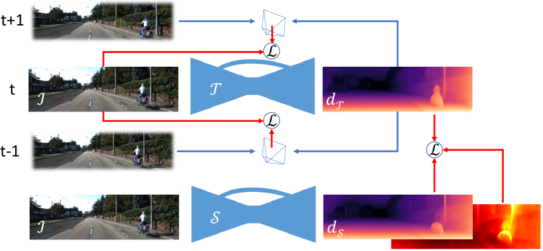
Figure 4: Self-Teaching scheme. A network $\mathcal{T}$ is trained in self-supervised fashion, e.g. on monocular sequences $[t-1,t,t+1]$. A new instance $\mathcal{S}$ of the same is trained on $d_{\mathcal{T}}$ output of $\mathcal{T}$.

Self-Teaching (Self). In order to decouple depth and pose when modelling uncertainty, we propose to source a direct form of supervision from the learned model itself. By training a first network in a self-supervised manner, we obtain a network instance $\mathcal{T}$ producing a noisy distribution $d_{\mathcal{T}}$. Then, we train a second instance of the same model, namely $\mathcal{S}$, to mimic the distribution sourced from $\mathcal{T}$. Typically, teacher-student frameworks [81] applied to monocular depth estimation [52] deploy a complex architecture to supervise a more compact one. In contrast, in our approach the teacher $\mathcal{T}$ and the student $\mathcal{S}$ share the same architecture and for this reason we refer to it as Self-Teaching (Self). By assuming an L1 loss, we can model for instance negative log-likelihood minimization as

$$\mathcal{L}_{\text{{Self}}}=\frac{|\mu(d_{\mathcal{S}})-d_{\mathcal{T}}|}{\sigma(d_{\mathcal{S}})}+\log\sigma(d_{\mathcal{S}})$$ (14)

We will show how with this strategy i) we obtain a network $\mathcal{S}$ more accurate than $\mathcal{T}$ and ii) in case of monocular supervision, we can decouple depth from pose and achieve a much more effective uncertainty estimation. Figure 4 summarizes our proposal.

3.4 Bayesian estimation

Finally, in Bayesian deep learning [29], the model uncertainty can be explained by marginalizing over all possible $w$ rather than choosing a point estimate. According to Neal [48], an approximate solution can be obtained by sampling N models and by modelling mean and variance as

$$p(d^{*}|\mathcal{I},\mathcal{D})\approx\sum_{i=1}^{N}p(d^{*}|\Theta(\mathcal{I},w_{i}))$$ (15)

If mean and variance are modelled for each $w_{i}$ sampling, we can obtain overall mean and variance as reported in [29, 27]

$$\mu(d)=\frac{1}{N}\sum_{i=1}^{N}\mu_{i}(d_{i})$$ (16)

$$\sigma^{2}(d)=\frac{1}{N}\sum_{i=1}^{N}(\mu_{i}(d_{i})-\mu(d))^{2}+\sigma_{i}^{2}(d_{i})$$ (17)

The implementation of this approximation is straightforward by combining empirical and predictive methods [29, 27]. Purposely, in our experiments we will pick the best empirical and predictive methods, e.g. combining Boot and Self (Boot+Self).

4 Experimental results

In this section, we exhaustively evaluate self-supervised strategies for joint depth and uncertainty estimation.

4.1 Evaluation protocol, dataset and metrics

At first, we describe all details concerning training and evaluation to ensure full reproducibility. Source code will be available at https://github.com/mattpoggi/mono-uncertainty.

Architecture and training schedule. We choose as baseline model Monodepth2 [20], thanks to the code made available and to its possibility to be trained seamlessly according to monocular, stereo, or both self-supervision paradigms. In our experiments, we train any variant of this method following the protocol defined in [20], on batches of 12 images resized to $192\times 640$ for 20 epochs starting from pre-trained encoders on ImageNet [12]. Moreover, we always follow the augmentation and training practices described in [20]. Finally, to evaluate Post we use the same weights made publicly available by the authors. Regarding empirical methods, we set $N$ to 8 and the number of cycles $C$ for Snap to 20. We randomly extract 25% of the training set for each independent network in Boot. Dropout is applied after convolutions in the decoder only. About predictive models, a single output channel is added in parallel to depth prediction channel.

Dataset. We compare all the models on the KITTI dataset [18], made of 61 scenes (about 42K stereo frames) acquired in driving scenarios. The dataset contains images at an average resolution of $375\times 1242$ and depth maps from a calibrated LiDAR sensor. Following standards in the field, we deploy the Eigen split [13] and set 80 meters as the maximum depth. For this purpose, we use the improved ground truth introduced in [68], much more accurate than the raw LiDAR data, since our aim is a strict evaluation rather than a comparison with existing monocular methods. Nevertheless, we report results on the raw LiDAR data using Garg’s crop [17] as well in the supplementary material.

Depth metrics. To assess depth accuracy, we report for the sake of page limit three out of seven standard metrics defined in [13]. Specifically, we report the absolute relative error (Abs Rel), root mean square error (RMSE), and the amount of inliers ($\delta<1.25$). We refer the reader to [13] or supplementary material for a complete description of these metrics. They enable a compact evaluation concerning both relative (Abs Rel and $\delta<1.25$) and absolute (RMSE) errors. Moreover, we also report the number of training iterations (#Trn), parameters (#Par), and forwards (#Fwd) required at testing time to estimate depth. In the case of monocular supervision, we scale depth as in [82].

Uncertainty metrics. To evaluate how significant the modelled uncertainties are, we use sparsification plots as in [27]. Given an error metric $\epsilon$, we sort all pixels in each depth map in order of descending uncertainty. Then, we iteratively extract a subset of pixels (i.e., 2% in our experiments) and compute $\epsilon$ on the remaining to plot a curve, that is supposed to shrink if the uncertainty properly encodes the errors in the depth map. An ideal sparsification (oracle) is obtained by sorting pixels in descending order of the $\epsilon$ magnitude. In contrast, a random uncertainty can be modelled as a constant, giving no information about how to remove erroneous measurements and, thus, a flat curve. By plotting the difference between estimated and oracle sparsification, we can measure the Area Under the Sparsification Error (AUSE, the lower the better). Subtracting estimated sparsification from random one enables computing the Area Under the Random Gain (AURG, the higher the better). The former quantifies how close the estimate is to the oracle uncertainty, the latter how better (or worse, as we will see in some cases) it is compared to no modelling at all. We assume Abs Rel, RMSE or $\delta\geq 1.25$ (since $\delta<1.25$ defines an accuracy score) as $\epsilon$.

Method Sup #Trn #Par #Fwd Abs Rel RMSE $\delta<$1.25 Monodepth2 [20] M $1\times$ $1\times$ $1\times$ 0.090 3.942 0.914 Monodepth2-Post [20] M $1\times$ $1\times$ $2\times$ 0.088 3.841 0.917 Monodepth2-Drop M $1\times$ $1\times$ N$\times$ 0.101 4.146 0.892 Monodepth2-Boot M N$\times$ N$\times$ $1\times$ 0.092 3.821 0.911 Monodepth2-Snap M 1$\times$ N$\times$ $1\times$ 0.091 3.921 0.912 Monodepth2-Repr M $1\times$ $1\times$ $1\times$ 0.092 3.936 0.912 Monodepth2-Log M $1\times$ $1\times$ $1\times$ 0.091 4.052 0.910 Monodepth2-Self M (1+1)$\times$ $1\times$ $1\times$ 0.087 3.826 0.920 Monodepth2-Boot+Log M N$\times$ N$\times$ $1\times$ 0.092 3.850 0.910 Monodepth2-Boot+Self M (1+N)$\times$ N$\times$ $1\times$ 0.088 3.799 0.918 Monodepth2-Snap+Log M $1\times$ $1\times$ $1\times$ 0.092 3.961 0.911 Monodepth2-Snap+Self M (1+1)$\times$ 1$\times$ $1\times$ 0.088 3.832 0.919

a) Depth evaluation

Abs Rel RMSE $\delta\geq 1.25$ Method AUSE AURG AUSE AURG AUSE AURG Monodepth2-Post 0.044 0.012 2.864 0.412 0.056 0.022 Monodepth2-Drop 0.065 0.000 2.568 0.944 0.097 0.002 Monodepth2-Boot 0.058 0.001 3.982 -0.743 0.084 -0.001 Monodepth2-Snap 0.059 -0.001 3.979 -0.639 0.083 -0.002 Monodepth2-Repr 0.051 0.008 2.972 0.381 0.069 0.013 Monodepth2-Log 0.039 0.020 2.562 0.916 0.044 0.038 Monodepth2-Self 0.030 0.026 2.009 1.266 0.030 0.045 Monodepth2-Boot+Log 0.038 0.021 2.449 0.820 0.046 0.037 Monodepth2-Boot+Self 0.029 0.028 1.924 1.316 0.028 0.049 Monodepth2-Snap+Log 0.038 0.022 2.385 1.001 0.043 0.039 Monodepth2-Snap+Self 0.031 0.026 2.043 1.230 0.030 0.045

b) Uncertainty evaluation

Table 1: Quantitative results for monocular (M) supervision. Evaluation on Eigen split [13] with improved ground truth [68].

4.2 Monocular (M) supervision

Depth. Table 1a reports depth accuracy for Monodepth2 variants implementing the different uncertainty estimation strategies when trained with monocular supervision. We can notice how, in general, empirical methods fail at improving depth prediction on most metrics, with Drop having a large gap from the baseline. On the other hand, Boot and Snap slightly reduce RMSE. Predictive methods as well produce worse depth estimates, except the proposed Self method, which improves all the metrics compared to the baseline, even when post-processed. Regarding the Bayesian solutions, both Boot and Snap performs worse when combined with Log, while they are always improved by the proposed Self method.

Uncertainty. Table 1b resumes performance of modelled uncertainties at reducing errors on the estimated depth maps. Surprisingly, empirical methods rarely perform better than the Post solution. In particular, empirical methods alone fail at performing better than a random chance, except for Drop that, on the other hand, produces much worse depth maps. Predictive methods perform better, with Log and Self yielding the best results. Among them, our method outperforms Log by a notable margin. Combining empirical and predictive methods is beneficial, often improving over single choices. In particular, Boot+Self achieves the best overall results.

Summary. In general Self, combined with empirical methods, performs better for both depth accuracy and uncertainty modelling when dealing with M supervision, thanks to disentanglement between depth and pose. We believe that empirical methods performance can be ascribed to depth scale, being unknown during training.

Method Sup #Trn #Par #Fwd Abs Rel RMSE $\delta<$1.25 Monodepth2 [20] S $1\times$ $1\times$ $1\times$ 0.085 3.942 0.912 Monodepth2-Post [20] S $1\times$ $1\times$ $2\times$ 0.084 3.777 0.915 Monodepth2-Drop S $1\times$ $1\times$ N$\times$ 0.129 4.908 0.819 Monodepth2-Boot S N$\times$ N$\times$ $1\times$ 0.085 3.772 0.914 Monodepth2-Snap S $1\times$ N$\times$ $1\times$ 0.085 3.849 0.912 Monodepth2-Repr S $1\times$ $1\times$ $1\times$ 0.085 3.873 0.913 Monodepth2-Log S $1\times$ $1\times$ $1\times$ 0.085 3.860 0.915 Monodepth2-Self S (1+1)$\times$ $1\times$ $1\times$ 0.084 3.835 0.915 Monodepth2-Boot+Log S N$\times$ N$\times$ $1\times$ 0.085 3.777 0.913 Monodepth2-Boot+Self S (1+N)$\times$ N$\times$ $1\times$ 0.085 3.793 0.914 Monodepth2-Snap+Log S 1$\times$ 1$\times$ $1\times$ 0.083 3.833 0.914 Monodepth2-Snap+Self S (1+1)$\times$ 1$\times$ $1\times$ 0.086 3.859 0.912

a) Depth evaluation

Abs Rel RMSE $\delta\geq 1.25$ Method AUSE AURG AUSE AURG AUSE AURG Monodepth2-Post 0.036 0.020 2.523 0.736 0.044 0.034 Monodepth2-Drop 0.103 -0.029 6.163 -2.169 0.231 -0.080 Monodepth2-Boot 0.028 0.029 2.291 0.964 0.031 0.048 Monodepth2-Snap 0.028 0.029 2.252 1.077 0.030 0.051 Monodepth2-Repr 0.040 0.017 2.275 1.074 0.050 0.030 Monodepth2-Log 0.022 0.036 0.938 2.402 0.018 0.061 Monodepth2-Self 0.022 0.035 1.679 1.642 0.022 0.056 Monodepth2-Boot+Log 0.020 0.038 0.807 2.455 0.018 0.063 Monodepth2-Boot+Self 0.023 0.035 1.646 1.628 0.021 0.058 Monodepth2-Snap+Log 0.021 0.037 0.891 2.426 0.018 0.061 Monodepth2-Snap+Self 0.023 0.035 1.710 1.623 0.023 0.058

b) Uncertainty evaluation

Table 2: Quantitative results for stereo (S) supervision. Evaluation on Eigen split [13] with improved ground truth [68].

4.3 Stereo (S) supervision

Depth. On Table 2a we show the results of the same approaches when trained with stereo supervision. Again, Drop fails to improve depth accuracy, together with Repr among predictive methods. Boot produces the best improvement, in particular in terms of RMSE. Traditional Log improves this time over the baseline, according to RMSE and $\delta<1.25$ metrics while, Self consistently improves the baseline on all metrics, although it does not outperform Post, which requires two forward passes.

Uncertainty. Table 2b summarizes the effectiveness of modelled uncertainties. This time, only Drop performs worse than Post achieving negative AURG, thus being detrimental at sparsification, while other empirical methods achieve much better results. In these experiments, thanks to the known pose of the stereo setup, Log deals only with depth uncertainty and thus performs extremely well. Self, although allowing for more accurate depth as reported in Table 2a, ranks second this time. Considering Bayesian implementations, again, both Boot and Snap are always improved. Conversely, compared to the M case, Log this time consistently outperforms Self in any Bayesian formulation.

Summary. When the pose is known, the gap between Log and Self concerning depth accuracy is minor, with Self performing better when modelling only predictive uncertainty and Log slightly better with Bayesian formulations. For uncertainty estimation, Log consistently performs better. The behavior of empirical methods alone confirms our findings from the previous experiments: by knowing the scale, Boot and Snap model uncertainty much better. In contrast, Drop fails for this purpose.

Method Sup #Trn #Par #Fwd Abs Rel RMSE $\delta<$1.25 Monodepth2 [20] MS $1\times$ $1\times$ $1\times$ 0.084 3.739 0.918 Monodepth2-Post [20] MS $1\times$ $1\times$ $2\times$ 0.082 3.666 0.919 Monodepth2-Drop MS $1\times$ 1$\times$ N$\times$ 0.172 5.885 0.679 Monodepth2-Boot MS N$\times$ N$\times$ 1$\times$ 0.086 3.787 0.910 Monodepth2-Snap MS $1\times$ N$\times$ $1\times$ 0.085 3.806 0.914 Monodepth2-Repr MS $1\times$ $1\times$ $1\times$ 0.084 3.828 0.913 Monodepth2-Log MS $1\times$ $1\times$ $1\times$ 0.083 3.790 0.916 Monodepth2-Self MS (1+1)$\times$ $1\times$ $1\times$ 0.083 3.682 0.919 Monodepth2-Boot+Log MS N$\times$ N$\times$ 1$\times$ 0.086 3.771 0.911 Monodepth2-Boot+Self MS (1+N)$\times$ N$\times$ 1$\times$ 0.085 3.704 0.915 Monodepth2-Snap+Log MS 1$\times$ 1$\times$ 1$\times$ 0.084 3.828 0.914 Monodepth2-Snap+Self MS (1+1)$\times$ 1$\times$ 1$\times$ 0.085 3.715 0.916

a) Depth evaluation

Abs Rel RMSE $\delta\geq 1.25$ Method AUSE AURG AUSE AURG AUSE AURG Monodepth2-Post 0.036 0.018 2.498 0.655 0.044 0.031 Monodepth2-Drop 0.103 -0.027 7.114 -2.580 0.303 -0.081 Monodepth2-Boot 0.028 0.030 2.269 0.985 0.034 0.049 Monodepth2-Snap 0.029 0.028 2.245 1.029 0.033 0.047 Monodepth2-Repr 0.046 0.010 2.662 0.635 0.062 0.018 Monodepth2-Log 0.028 0.029 1.714 1.562 0.028 0.050 Monodepth2-Self 0.022 0.033 1.654 1.515 0.023 0.052 Monodepth2-Boot+Log 0.030 0.028 1.962 1.282 0.032 0.051 Monodepth2-Boot+Self 0.023 0.033 1.688 1.494 0.023 0.056 Monodepth2-Snap+Log 0.030 0.027 2.032 1.272 0.032 0.048 Monodepth2-Snap+Self 0.023 0.034 1.684 1.510 0.023 0.055

b) Uncertainty evaluation

Table 3: Quantitative results for monocular+stereo (MS) supervision. Evaluation on Eigen split [13] with improved ground truth [68].

4.4 Monocular+Stereo (MS) supervision

Depth. Table 3a reports the behavior of depth accuracy when monocular and stereo supervisions are combined. In this case, only Self consistently outperforms the baseline and is competitive with Post, which still requires two forward passes. Among empirical methods, Boot is the most effective. Regarding Bayesian solutions, those using Self are, in general, more accurate on most metrics, yet surprisingly worse than Self alone.

Uncertainty. Table 3b shows the performance of the considered uncertainties. The behavior of all variants is similar to the one observed with stereo supervision, except for Log and Self. We can notice that Self outperforms Log, similarly to what observed with M supervision. It confirms that pose estimation drives Log to worse uncertainty estimation, while Self models are much better thanks to the training on proxy labels produced by the Teacher network. Concerning Bayesian solutions, in general, Boot and Snap are improved when combined with both Log and Self, with Self combinations typically better than their Log counterparts and equivalent to standalone Self.

Summary. The evaluation with monocular and stereo supervision confirms that when the pose is estimated alongside with depth, Self proves to be a better solution compared to Log and, in general, other approaches to model uncertainty. Finally, empirical methods alone behave as for experiments with stereo supervision, confirming that the knowledge of the scale during training is crucial to the proper behavior of Drop, Boot and Snap.

4.5 Sparsification curves

In order to further outline our findings, we report in Figure 5 the RMSE sparsification error curves, averaged over the test set, when training with M, S or MS supervision. The plots show that methods leveraging on Self (blue) are the best to model uncertainty when dealing with pose estimation, i.e. M and MS, while those using Log (green) are better when training on S. We report curves for Abs Rel and $\delta\geq 1.25$ in the supplementary material.

4.6 Supplementary material

For the sake of the pages limit, we report more details about the experiments shown so far in the supplementary material. Specifically, i) complete depth evaluation with all seven metrics defined in [13], ii) depth and uncertainty evaluation with reduced depth range to 50 meters, iii) evaluation assuming the raw LiDAR data as ground truth, for compliancy with previous works [20] and iv) sparsification curves for all metrics. We also provide additional qualitative results in the form of images and a video sequence, available at www.youtube.com/watch?v=bxVPXqf4zt4.

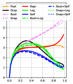
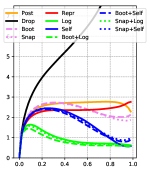
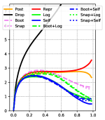
Figure 5: Sparsification Error curves. From left to right, average RMSE with M, S and MS supervisions. Best viewed with colors.

5 Conclusion

In this paper, we have thoroughly investigated for the first time in literature uncertainty modelling in self-supervised monocular depth estimation. We have reviewed and evaluated existing techniques, as well as introduced a novel Self-Teaching (Self) paradigm. We have considered up to 11 strategies to estimate the uncertainty on predictions of a depth-from-mono network trained in a self-supervised manner. Our experiments highlight how different supervision strategies lead to different winners among the considered methods. In particular, among empirical methods, only Dropout sampling performs well when the scale is unknown during training (M), while it is the only one failing when scale is known (S, MS). Empirical methods are affected by pose estimation, for which log-likelihood maximization gives sub-optimal results when the pose is unknown (M, MS). In these latter cases, potentially the most appealing for practical applications, the proposed Self technique results in the best strategy to model uncertainty. Moreover, uncertainty estimation also improves depth accuracy consistently, with any training paradigm.

Acknowledgement. We gratefully acknowledge the support of NVIDIA Corporation with the donation of the Titan Xp GPU used for this research.

Supplementary See supplementary.pdf See supplementary.pdf See supplementary.pdf See supplementary.pdf See supplementary.pdf See supplementary.pdf See supplementary.pdf See supplementary.pdf See supplementary.pdf See supplementary.pdf See supplementary.pdf See supplementary.pdf See supplementary.pdf See supplementary.pdf See supplementary.pdf

References

- [1] Filippo Aleotti, Fabio Tosi, Matteo Poggi, and Stefano Mattoccia. Generative adversarial networks for unsupervised monocular depth prediction. In 15th European Conference on Computer Vision (ECCV) Workshops, 2018.
- [2] Lorenzo Andraghetti, Panteleimon Myriokefalitakis, Pier Luigi Dovesi, Belen Luque, Matteo Poggi, Alessandro Pieropan, and Stefano Mattoccia. Enhancing self-supervised monocular depth estimation with traditional visual odometry. In 7th International Conference on 3D Vision (3DV), 2019.
- [3] Ranjan Anurag, Varun Jampani, Kihwan Kim, Deqing Sun, Jonas Wulff, and Michael J. Black. Competitive collaboration: Joint unsupervised learning of depth, camera motion, optical flow and motion segmentation. In The IEEE Conference on Computer Vision and Pattern Recognition (CVPR), 2019.
- [4] Amir Atapour-Abarghouei and Toby P Breckon. Real-time monocular depth estimation using synthetic data with domain adaptation via image style transfer. In Proceedings of the IEEE Conference on Computer Vision and Pattern Recognition, volume 18, page 1, 2018.
- [5] Jia-Wang Bian, Zhichao Li, Naiyan Wang, Huangying Zhan, Chunhua Shen, Ming-Ming Cheng, and Ian Reid. Unsupervised scale-consistent depth and ego-motion learning from monocular video. In Thirty-third Conference on Neural Information Processing Systems (NeurIPS), 2019.
- [6] Charles Blundell, Julien Cornebise, Koray Kavukcuoglu, and Daan Wierstra. Weight uncertainty in neural networks. arXiv preprint arXiv:1505.05424, 2015.
- [7] Andrés Bruhn and Joachim Weickert. A confidence measure for variational optic flow methods. In Geometric Properties for Incomplete Data, pages 283–298. Springer, 2006.
- [8] Vincent Casser, Soeren Pirk, Reza Mahjourian, and Anelia Angelova. Depth prediction without the sensors: Leveraging structure for unsupervised learning from monocular videos. In Thirty-Third AAAI Conference on Artificial Intelligence (AAAI-19), 2019.
- [9] Long Chen, Wen Tang, and Nigel John. Self-supervised monocular image depth learning and confidence estimation. arXiv preprint arXiv:1803.05530, 2018.
- [10] Tianqi Chen, Emily Fox, and Carlos Guestrin. Stochastic gradient hamiltonian monte carlo. In International conference on machine learning, pages 1683–1691, 2014.
- [11] Yuhua Chen, Cordelia Schmid, and Cristian Sminchisescu. Self-supervised learning with geometric constraints in monocular video: Connecting flow, depth, and camera. In ICCV, 2019.
- [12] Jia Deng, Wei Dong, Richard Socher, Li-Jia Li, Kai Li, and Li Fei-Fei. Imagenet: A large-scale hierarchical image database. In 2009 IEEE conference on computer vision and pattern recognition, pages 248–255. Ieee, 2009.
- [13] David Eigen, Christian Puhrsch, and Rob Fergus. Depth map prediction from a single image using a multi-scale deep network. In Advances in neural information processing systems, pages 2366–2374, 2014.
- [14] Sean Fanello, Cem Keskin, Shahram Izadi, Pushmeet Kohli, David Kim, David Sweeney, Antonio Criminisi, Jamie Shotton, Sing Bing Kang, and Tim Paek. Learning to be a depth camera for close-range human capture and interaction. ACM Transactions on Graphics (TOG) - Proceedings of ACM SIGGRAPH 2014, 33, July 2014.
- [15] Huan Fu, Mingming Gong, Chaohui Wang, Kayhan Batmanghelich, and Dacheng Tao. Deep ordinal regression network for monocular depth estimation. In The IEEE Conference on Computer Vision and Pattern Recognition (CVPR), 2018.
- [16] Yarin Gal and Zoubin Ghahramani. Dropout as a bayesian approximation: Representing model uncertainty in deep learning. In international conference on machine learning, pages 1050–1059, 2016.
- [17] Ravi Garg, Vijay Kumar BG, Gustavo Carneiro, and Ian Reid. Unsupervised cnn for single view depth estimation: Geometry to the rescue. In European Conference on Computer Vision, pages 740–756. Springer, 2016.
- [18] Andreas Geiger, Philip Lenz, Christoph Stiller, and Raquel Urtasun. Vision meets robotics: The kitti dataset. The International Journal of Robotics Research, 32(11):1231–1237, 2013.
- [19] Clément Godard, Oisin Mac Aodha, and Gabriel J. Brostow. Unsupervised monocular depth estimation with left-right consistency. In CVPR, 2017.
- [20] Clement Godard, Oisin Mac Aodha, Michael Firman, and Gabriel J. Brostow. Digging into self-supervised monocular depth estimation. In The IEEE International Conference on Computer Vision (ICCV), October 2019.
- [21] Alex Graves. Practical variational inference for neural networks. In Advances in neural information processing systems, pages 2348–2356, 2011.
- [22] Xiaoyang Guo, Hongsheng Li, Shuai Yi, Jimmy Ren, and Xiaogang Wang. Learning monocular depth by distilling cross-domain stereo networks. In Proceedings of the European Conference on Computer Vision (ECCV), pages 484–500, 2018.
- [23] Heiko Hirschmüller. Stereo processing by semiglobal matching and mutual information. PAMI, 30(2):328–341, 2008.
- [24] Xiaoyan Hu and Philippos Mordohai. A quantitative evaluation of confidence measures for stereo vision. PAMI, 34(11):2121–2133, 2012.
- [25] Gao Huang, Yixuan Li, Geoff Pleiss, Zhuang Liu, John E Hopcroft, and Kilian Q Weinberger. Snapshot ensembles: Train 1, get m for free. In ICLR, 2017.
- [26] Po-Yu Huang, Wan-Ting Hsu, Chun-Yueh Chiu, Ting-Fan Wu, and Min Sun. Efficient uncertainty estimation for semantic segmentation in videos. In Proceedings of the European Conference on Computer Vision (ECCV), pages 520–535, 2018.
- [27] Eddy Ilg, Ozgun Cicek, Silvio Galesso, Aaron Klein, Osama Makansi, Frank Hutter, and Thomas Brox. Uncertainty estimates and multi-hypotheses networks for optical flow. In Proceedings of the European Conference on Computer Vision (ECCV), pages 652–667, 2018.
- [28] Eddy Ilg, Nikolaus Mayer, Tonmoy Saikia, Margret Keuper, Alexey Dosovitskiy, and Thomas Brox. Flownet 2.0: Evolution of optical flow estimation with deep networks. In CVPR, pages 2462–2470, 2017.
- [29] Alex Kendall and Yarin Gal. What uncertainties do we need in bayesian deep learning for computer vision? In Advances in neural information processing systems, pages 5574–5584, 2017.
- [30] Alex Kendall, Yarin Gal, and Roberto Cipolla. Multi-task learning using uncertainty to weight losses for scene geometry and semantics. In Proceedings of the IEEE Conference on Computer Vision and Pattern Recognition, pages 7482–7491, 2018.
- [31] Sunok Kim, Seungryong Kim, Dongbo Min, and Kwanghoon Sohn. Laf-net: Locally adaptive fusion networks for stereo confidence estimation. In The IEEE Conference on Computer Vision and Pattern Recognition (CVPR), June 2019.
- [32] Maria Klodt and Andrea Vedaldi. Supervising the new with the old: learning sfm from sfm. In The European Conference on Computer Vision (ECCV), September 2018.
- [33] Claudia Kondermann, Daniel Kondermann, Bernd Jähne, and Christoph Garbe. An adaptive confidence measure for optical flows based on linear subspace projections. In Joint Pattern Recognition Symposium, pages 132–141. Springer, 2007.
- [34] Claudia Kondermann, Rudolf Mester, and Christoph Garbe. A statistical confidence measure for optical flows. In European Conference on Computer Vision, pages 290–301. Springer, 2008.
- [35] Yevhen Kuznietsov, Jorg Stuckler, and Bastian Leibe. Semi-supervised deep learning for monocular depth map prediction. In The IEEE Conference on Computer Vision and Pattern Recognition (CVPR), July 2017.
- [36] Jan Kybic and Claudia Nieuwenhuis. Bootstrap optical flow confidence and uncertainty measure. Computer Vision and Image Understanding, 115(10):1449–1462, 2011.
- [37] Lubor Ladicky, Jianbo Shi, and Marc Pollefeys. Pulling things out of perspective. In Proceedings of the IEEE Conference on Computer Vision and Pattern Recognition, pages 89–96, 2014.
- [38] Iro Laina, Christian Rupprecht, Vasileios Belagiannis, Federico Tombari, and Nassir Navab. Deeper depth prediction with fully convolutional residual networks. In 2016 Fourth international conference on 3D vision (3DV), pages 239–248. IEEE, 2016.
- [39] Balaji Lakshminarayanan, Alexander Pritzel, and Charles Blundell. Simple and scalable predictive uncertainty estimation using deep ensembles. In Advances in Neural Information Processing Systems, pages 6402–6413, 2017.
- [40] Fayao Liu, Chunhua Shen, Guosheng Lin, and Ian Reid. Learning depth from single monocular images using deep convolutional neural fields. IEEE transactions on pattern analysis and machine intelligence, 38(10):2024–2039, 2016.
- [41] Chenxu Luo, Zhenheng Yang, Peng Wang, Yang Wang, Wei Xu, Ram Nevatia, and Alan Yuille. Every pixel counts++: Joint learning of geometry and motion with 3d holistic understanding. PAMI, 2019.
- [42] Yue Luo, Jimmy Ren, Mude Lin, Jiahao Pang, Wenxiu Sun, Hongsheng Li, and Liang Lin. Single view stereo matching. In Proceedings of the IEEE Conference on Computer Vision and Pattern Recognition, pages 155–163, 2018.
- [43] Oisin Mac Aodha, Ahmad Humayun, Marc Pollefeys, and Gabriel J Brostow. Learning a confidence measure for optical flow. IEEE transactions on pattern analysis and machine intelligence, 35(5):1107–1120, 2012.
- [44] David JC MacKay. A practical bayesian framework for backpropagation networks. Neural computation, 4(3):448–472, 1992.
- [45] Reza Mahjourian, Martin Wicke, and Anelia Angelova. Unsupervised learning of depth and ego-motion from monocular video using 3d geometric constraints. In The IEEE Conference on Computer Vision and Pattern Recognition (CVPR), 2018.
- [46] Nikolaus Mayer, Eddy Ilg, Philip Hausser, Philipp Fischer, Daniel Cremers, Alexey Dosovitskiy, and Thomas Brox. A large dataset to train convolutional networks for disparity, optical flow, and scene flow estimation. In CVPR, pages 4040–4048, 2016.
- [47] Pushmeet Kohli Nathan Silberman, Derek Hoiem and Rob Fergus. Indoor segmentation and support inference from rgbd images. In ECCV, 2012.
- [48] Radford M Neal. Bayesian learning for neural networks, volume 118. Springer Science & Business Media, 2012.
- [49] David A Nix and Andreas S Weigend. Estimating the mean and variance of the target probability distribution. In Proceedings of 1994 IEEE International Conference on Neural Networks (ICNN’94), volume 1, pages 55–60. IEEE, 1994.
- [50] Valentino Peluso, Antonio Cipolletta, Andrea Calimera, Matteo Poggi, Fabio Tosi, and Stefano Mattoccia. Enabling energy-efficient unsupervised monocular depth estimation on armv7-based platforms. In Design Automation and Test in Europe (DATE 2019), 2019.
- [51] Sudeep Pillai, Rareş Ambruş, and Adrien Gaidon. Superdepth: Self-supervised, super-resolved monocular depth estimation. In 2019 International Conference on Robotics and Automation (ICRA), pages 9250–9256. IEEE, 2019.
- [52] Andrea Pilzer, Stephane Lathuiliere, Nicu Sebe, and Elisa Ricci. Refine and distill: Exploiting cycle-inconsistency and knowledge distillation for unsupervised monocular depth estimation. In The IEEE Conference on Computer Vision and Pattern Recognition (CVPR), 2019.
- [53] Matteo Poggi, Filippo Aleotti, Fabio Tosi, and Stefano Mattoccia. Towards real-time unsupervised monocular depth estimation on cpu. In IEEE/JRS Conference on Intelligent Robots and Systems (IROS), 2018.
- [54] Matteo Poggi and Stefano Mattoccia. Learning from scratch a confidence measure. In BMVC, 2016.
- [55] Matteo Poggi, Fabio Tosi, and Stefano Mattoccia. Quantitative evaluation of confidence measures in a machine learning world. In ICCV, pages 5228–5237, 2017.
- [56] Matteo Poggi, Fabio Tosi, and Stefano Mattoccia. Learning monocular depth estimation with unsupervised trinocular assumptions. In 6th International Conference on 3D Vision (3DV), 2018.
- [57] Ashutosh Saxena, Min Sun, and Andrew Y Ng. Make3d: Learning 3d scene structure from a single still image. IEEE transactions on pattern analysis and machine intelligence, 31(5):824–840, 2008.
- [58] Ashutosh Saxena, Min Sun, and Andrew Y Ng. Make3d: Learning 3d scene structure from a single still image. IEEE transactions on pattern analysis and machine intelligence, 31(5):824–840, 2009.
- [59] Daniel Scharstein and Richard Szeliski. A taxonomy and evaluation of dense two-frame stereo correspondence algorithms. IJCV, 47(1-3):7–42, 2002.
- [60] Steven M Seitz, Brian Curless, James Diebel, Daniel Scharstein, and Richard Szeliski. A comparison and evaluation of multi-view stereo reconstruction algorithms. In 2006 IEEE Computer Society Conference on Computer Vision and Pattern Recognition (CVPR’06), volume 1, pages 519–528. IEEE, 2006.
- [61] Akihito Seki and Marc Pollefeys. Patch based confidence prediction for dense disparity map. In BMVC, volume 2, page 4, 2016.
- [62] Amit Shaked and Lior Wolf. Improved stereo matching with constant highway networks and reflective confidence learning. In CVPR, pages 4641–4650, 2017.
- [63] Nitish Srivastava, Geoffrey Hinton, Alex Krizhevsky, Ilya Sutskever, and Ruslan Salakhutdinov. Dropout: a simple way to prevent neural networks from overfitting. The journal of machine learning research, 15(1):1929–1958, 2014.
- [64] Alessio Tonioni, Matteo Poggi, Stefano Mattoccia, and Luigi Di Stefano. Unsupervised domain adaptation for depth prediction from images. IEEE Transactions on Pattern Analysis and Machine Intelligence, 2019. Available at https://ieeexplore.ieee.org/document/8834825.
- [65] Fabio Tosi, Filippo Aleotti, Matteo Poggi, and Stefano Mattoccia. Learning monocular depth estimation infusing traditional stereo knowledge. In The IEEE Conference on Computer Vision and Pattern Recognition (CVPR), 2019.
- [66] Fabio Tosi, Filippo Aleotti, Pierluigi Zama Ramirez, Matteo Poggi, Samuele Salti, Luigi Di Stefano, and Stefano Mattoccia. Distilled semantics for comprehensive scene understanding from videos. In The IEEE Conference on Computer Vision and Pattern Recognition (CVPR), 2020.
- [67] Fabio Tosi, Matteo Poggi, Antonio Benincasa, and Stefano Mattoccia. Beyond local reasoning for stereo confidence estimation with deep learning. In ECCV, pages 319–334, 2018.
- [68] Jonas Uhrig, Nick Schneider, Lukas Schneider, Uwe Franke, Thomas Brox, and Andreas Geiger. Sparsity invariant cnns. In International Conference on 3D Vision (3DV), pages 11–20. IEEE, 2017.
- [69] Chaoyang Wang, Jose Miguel Buenaposada, Rui Zhu, and Simon Lucey. Learning depth from monocular videos using direct methods. In The IEEE Conference on Computer Vision and Pattern Recognition (CVPR), 2018.
- [70] Zhou Wang, A. C. Bovik, H. R. Sheikh, and E. P. Simoncelli. Image quality assessment: From error visibility to structural similarity. Trans. Img. Proc., 13(4):600–612, Apr. 2004.
- [71] Anne S Wannenwetsch, Margret Keuper, and Stefan Roth. Probflow: Joint optical flow and uncertainty estimation. In Proceedings of the IEEE International Conference on Computer Vision, pages 1173–1182, 2017.
- [72] Jamie Watson, Michael Firman, Gabriel J. Brostow, and Daniyar Turmukhambetov. Self-supervised monocular depth hints. In The IEEE International Conference on Computer Vision (ICCV), October 2019.
- [73] Max Welling and Yee W Teh. Bayesian learning via stochastic gradient langevin dynamics. In Proceedings of the 28th international conference on machine learning (ICML-11), pages 681–688, 2011.
- [74] Dan Xu, Wei Wang, Hao Tang, Hong Liu, Nicu Sebe, and Elisa Ricci. Structured attention guided convolutional neural fields for monocular depth estimation. In The IEEE Conference on Computer Vision and Pattern Recognition (CVPR), 2018.
- [75] Haofei Xu, Jianmin Zheng, Jianfei Cai, and Juyong Zhang. Region deformer networks for unsupervised depth estimation from unconstrained monocular videos. In IJCAI, 2019.
- [76] Nan Yang, Rui Wang, Jörg Stückler, and Daniel Cremers. Deep virtual stereo odometry: Leveraging deep depth prediction for monocular direct sparse odometry. In European Conference on Computer Vision, pages 835–852. Springer, 2018.
- [77] Zhenheng Yang, Peng Wang, Yang Wang, Wei Xu, and Ram Nevatia. Every pixel counts: Unsupervised geometry learning with holistic 3d motion understanding. In The European Conference on Computer Vision (ECCV) Workshops, September 2018.
- [78] Zhichao Yin and Jianping Shi. Geonet: Unsupervised learning of dense depth, optical flow and camera pose. In The IEEE Conference on Computer Vision and Pattern Recognition (CVPR), 2018.
- [79] Pierluigi Zama Ramirez, Matteo Poggi, Fabio Tosi, Stefano Mattoccia, and Luigi Di Stefano. Geometry meets semantic for semi-supervised monocular depth estimation. In 14th Asian Conference on Computer Vision (ACCV), 2018.
- [80] Huangying Zhan, Ravi Garg, Chamara Saroj Weerasekera, Kejie Li, Harsh Agarwal, and Ian Reid. Unsupervised learning of monocular depth estimation and visual odometry with deep feature reconstruction. In The IEEE Conference on Computer Vision and Pattern Recognition (CVPR), 2018.
- [81] Mengyu Zheng, Chuan Zhou, Jia Wu, and Li Guo. Smooth deep network embedding. In 2019 International Joint Conference on Neural Networks (IJCNN), pages 1–8. IEEE, 2019.
- [82] Tinghui Zhou, Matthew Brown, Noah Snavely, and David G Lowe. Unsupervised learning of depth and ego-motion from video. In CVPR, volume 2, page 7, 2017.
- [83] Yuliang Zou, Zelun Luo, and Jia-Bin Huang. Df-net: Unsupervised joint learning of depth and flow using cross-task consistency. In European Conference on Computer Vision, pages 38–55. Springer, 2018.
See supplementary.pdf See supplementary.pdf See supplementary.pdf See supplementary.pdf See supplementary.pdf See supplementary.pdf See supplementary.pdf See supplementary.pdf See supplementary.pdf See supplementary.pdf See supplementary.pdf See supplementary.pdf See supplementary.pdf See supplementary.pdf See supplementary.pdf