Inference on Achieved Signal Noise Ratio

Abstract

We describe a procedure to perform approximate inference on the achieved signal-noise ratio of the Markowitz portfolio under Gaussian i.i.d. returns. The procedure relies on a statistic similar to the Sharpe Ratio Information Criterion. [8] Testing indicates the procedure is somewhat conservative, but otherwise works well for reasonable values of sample and asset universe sizes. We adapt the procedure to deal with generalizations of the portfolio optimization problem.

1 Introduction

For a universe of $k$ assets, we consider the portfolio optimization problem

$$\max_{\boldsymbol{\nu}}\frac{{{\boldsymbol{\nu}}^{\top}}\boldsymbol{\mu}}{\sqrt{{{\boldsymbol{\nu}}^{\top}}\mathsf{\Sigma}\boldsymbol{\nu}}}.$$ (1)

Here $\boldsymbol{\mu}$ is the expected return and $\mathsf{\Sigma}$ is the covariance of returns. This problem is solved by the Markowitz portfolio, defined as

$${{\boldsymbol{\nu}}_{{}*}}=_{\operatorname{df}}{{\mathsf{\Sigma}}^{-1}}{\boldsymbol{\mu}},$$ (2)

and any positive multiple thereof.

In practice the parameters $\boldsymbol{\mu}$ and $\mathsf{\Sigma}$ are unknown and must be estimated from the data. The estimation of parameters is known to deterioriate the quality of the portfolio. [7] The signal-noise ratio of the Markowitz portfolio, its mean divided by its volatility, is subject to a fundamental bound. [10, 2] While inference on the population parameters follows from classical statistics via the connection to Hotelling’s $T^{2}$, little is known about performing inference on the signal-noise ratio achieved by the Markowitz portfolio. Paulsen and Söhl described the Sharpe Ratio Information Criterion (SRIC), which is an approximately unbiased estimator for this quantity. [8] Some asymptotic confidence intervals have also been described, but these require unreasonably large sample sizes. [9] Here we fill this gap, describing confidence intervals very similar to the SRIC and using the same approximation. Practical construction of these bounds requires one to estimate the population effect size. In practice this causes the confidence intervals to be slightly conservative.

2 The Procedure

Assume you observe returns on $k$ assets, which are independently drawn from a Gaussian distribution ${{x}_{t}}\sim\mathcal{N}\left(\boldsymbol{\mu},\mathsf{\Sigma}\right)$. The population Markowitz portfolio is ${{\boldsymbol{\nu}}_{{}*}}={{\mathsf{\Sigma}}^{-1}}\boldsymbol{\mu}$. The signal-noise ratio of this portfolio is ${\zeta}_{*}=\sqrt{{{\boldsymbol{\mu}}^{\top}}{{\mathsf{\Sigma}}^{-1}}\boldsymbol{\mu}}$. Given $n$ observations of returns, one typically estimates the population parameters via

$$\boldsymbol{\hat{\mu}} =\frac{1}{n}\sum_{1\leq t\leq n}{{x}_{t}},$$ (3)

$$\mathsf{\hat{\Sigma}} =\frac{1}{n-1}\sum_{1\leq t\leq n}{{x}_{t}}{{{{x}_{t}}}^{\top}}-\frac{n}{n-1}\boldsymbol{\hat{\mu}}{{\boldsymbol{\hat{\mu}}}^{\top}}.$$ (4)

The (sample) Markowitz portfolio is ${{\boldsymbol{\hat{\nu}}}_{{}*}}={{\mathsf{\hat{\Sigma}}}^{-1}}\boldsymbol{\hat{\mu}}$. The achieved signal-noise ratio of ${{\boldsymbol{\hat{\nu}}}_{{}*}}$ is defined as

$${\zeta}_{a}=_{\operatorname{df}}\frac{{{\boldsymbol{\mu}}^{\top}}{{\boldsymbol{\hat{\nu}}}_{{}*}}}{\sqrt{{{{{\boldsymbol{\hat{\nu}}}_{{}*}}}^{\top}}\mathsf{\Sigma}{{\boldsymbol{\hat{\nu}}}_{{}*}}}}.$$ (5)

It is an unobservable random quantity that we wish to perform inference on.

The Sharpe ratio of ${{\boldsymbol{\hat{\nu}}}_{{}*}}$ is defined as

$${\hat{\zeta}}_{*}=_{\operatorname{df}}\frac{{{\boldsymbol{\hat{\mu}}}^{\top}}{{\boldsymbol{\hat{\nu}}}_{{}*}}}{\sqrt{{{{{\boldsymbol{\hat{\nu}}}_{{}*}}}^{\top}}\mathsf{\hat{\Sigma}}{{\boldsymbol{\hat{\nu}}}_{{}*}}}}=\sqrt{{{\boldsymbol{\hat{\mu}}}^{\top}}{{\mathsf{\hat{\Sigma}}}^{-1}}\boldsymbol{\hat{\mu}}}.$$ (6)

We note that $T^{2}=n{\hat{\zeta}}^{2}_{*}$ is the familiar Hotelling’s statistic, which is usually prescribed to perform inference on $\boldsymbol{\mu}$, but can be used to perform inference on ${\zeta}^{2}_{*}$. [1, 11]

The Sharpe Ratio Information Criterion is defined as [8]

$$SRIC=_{\operatorname{df}}{\hat{\zeta}}_{*}-\frac{k-1}{n{\hat{\zeta}}_{*}}.$$ (7)

Under the simplifying approximation

$$\mathsf{\hat{\Sigma}}\approx\mathsf{\Sigma},$$ (8)

the SRIC is unbiased for the achieved signal-noise ratio:

$$\operatorname{E}\left[SRIC\right]=\operatorname{E}\left[{\zeta}_{a}\right].$$ (9)

Note this only holds for $k>1$, but it is simple to express $\operatorname{E}\left[{\zeta}_{a}\right]$ when $k=1$.

Inspired by the SRIC, we seek a constant ${{c}_{\alpha}}$ such that

$$\operatorname{Pr}\left\{{\zeta}_{a}\leq{\hat{\zeta}}_{*}-\frac{{{c}_{\alpha}}}{n{\hat{\zeta}}_{*}}\right\}=\alpha.$$ (10)

Under Approximation 8,

$${\zeta}_{a}\approx\frac{{{\boldsymbol{\mu}}^{\top}}{{\mathsf{\Sigma}}^{-1}}\boldsymbol{\hat{\mu}}}{\sqrt{{{\left({{\mathsf{\Sigma}}^{-1}}\boldsymbol{\hat{\mu}}\right)}^{\top}}\mathsf{\Sigma}\left({{\mathsf{\Sigma}}^{-1}}\boldsymbol{\hat{\mu}}\right)}}=\frac{{{\boldsymbol{\mu}}^{\top}}{{\mathsf{\Sigma}}^{-1}}\boldsymbol{\hat{\mu}}}{\sqrt{{{\boldsymbol{\hat{\mu}}}^{\top}}{{\mathsf{\Sigma}}^{-1}}\boldsymbol{\hat{\mu}}}}=\frac{{{\boldsymbol{\mu}}^{\top}}{{\mathsf{\Sigma}}^{-1}}\boldsymbol{\hat{\mu}}}{{\hat{\zeta}}_{*}}.$$ (11)

Under the approximation we also have ${\hat{\zeta}}^{2}_{*}\approx{{\boldsymbol{\hat{\mu}}}^{\top}}{{\mathsf{\Sigma}}^{-1}}\boldsymbol{\hat{\mu}}$. We note that for Gaussian returns, we can write

$$\boldsymbol{\hat{\mu}}=\boldsymbol{\mu}+\frac{1}{\sqrt{n}}{{\mathsf{\Sigma}}^{1/2}}\boldsymbol{z},$$

where $\boldsymbol{z}\sim\mathcal{N}\left(\boldsymbol{0},\mathsf{I}\right).$ Thus

$${\hat{\zeta}}^{2}_{*}-{\zeta}_{a}{\hat{\zeta}}_{*} \approx{{\boldsymbol{\hat{\mu}}}^{\top}}{{\mathsf{\Sigma}}^{-1}}\boldsymbol{\hat{\mu}}-{{\boldsymbol{\mu}}^{\top}}{{\mathsf{\Sigma}}^{-1}}\boldsymbol{\hat{\mu}},$$

$$={{\left(\boldsymbol{\hat{\mu}}-\boldsymbol{\mu}\right)}^{\top}}{{\mathsf{\Sigma}}^{-1}}\boldsymbol{\hat{\mu}},$$

$$=\frac{1}{n}{{\boldsymbol{z}}^{\top}}{{\mathsf{\Sigma}}^{\top/2}}{{\mathsf{\Sigma}}^{-1}}\left(\sqrt{n}\boldsymbol{\mu}+{{\mathsf{\Sigma}}^{1/2}}\boldsymbol{z}\right),$$

$$=\frac{1}{n}{{\boldsymbol{z}}^{\top}}\left(\sqrt{n}{{\mathsf{\Sigma}}^{-1/2}}\boldsymbol{\mu}+\boldsymbol{z}\right),$$

$$=\frac{1}{n}{{\left(\frac{1}{2}\sqrt{n}{{\mathsf{\Sigma}}^{-1/2}}\boldsymbol{\mu}+\boldsymbol{z}-\frac{1}{2}\sqrt{n}{{\mathsf{\Sigma}}^{-1/2}}\boldsymbol{\mu}\right)}^{\top}}\left(\frac{1}{2}\sqrt{n}{{\mathsf{\Sigma}}^{-1/2}}\boldsymbol{\mu}+\boldsymbol{z}+\frac{1}{2}\sqrt{n}{{\mathsf{\Sigma}}^{-1/2}}\boldsymbol{\mu}\right),$$

$$=\frac{1}{n}\left(\left\|{\frac{1}{2}\sqrt{n}{{\mathsf{\Sigma}}^{-1/2}}\boldsymbol{\mu}+\boldsymbol{z}}\right\|_{2}^{2}-\left\|{\frac{1}{2}\sqrt{n}{{\mathsf{\Sigma}}^{-1/2}}\boldsymbol{\mu}}\right\|_{2}^{2}\right),$$

$$\sim\frac{1}{n}\left(\chi^{2}\left(k,\frac{n{\zeta}^{2}_{*}}{4}\right)-\frac{n{\zeta}^{2}_{*}}{4}\right).$$

Now because

$${\zeta}_{a}\leq{\hat{\zeta}}_{*}-\frac{c}{n{\hat{\zeta}}_{*}}\Leftrightarrow c\leq n\left({\hat{\zeta}}^{2}_{*}-{\zeta}_{a}{\hat{\zeta}}_{*}\right),$$

If we want this condition to hold with probability $\alpha$ we should set

$${{c}_{\alpha}}={{{\chi^{2}}_{1-\alpha}}\left(k,\frac{n{\zeta}^{2}_{*}}{4}\right)-\frac{n{\zeta}^{2}_{*}}{4}},$$ (12)

where ${{\chi^{2}}_{q}}\left(v,\delta\right)$ is the $q$ quantile of the non-central chi-square distribution with $v$ degrees of freedom and non-centrality parameter $\delta$.

Checking coverage

Before proceeding, we check whether use of Approximation 8 leads to a degradation in coverage of a confidence interval implied by Inequality 10. We draw $n$ days of returns from the $k$-variate normal distribution. For a fixed value of ${\zeta}_{*}$, we perform $1,000,000$ simulations of computing ${\zeta}_{a}$ and ${\hat{\zeta}}^{2}_{*}$, computing a one-sided confidence bound and measuring the empirical rate of type I errors. We then let $n$ vary from 50 to $102,400$ days; we let $k$ vary from 2 to 16; we let ${\zeta}_{*}$ vary from $0.5\,{{\mbox{yr}}^{-1/2}}$ to $2\,{{\mbox{yr}}^{-1/2}}$, where we assume 252 days per year. We compute the lower confidence limit on ${\zeta}_{a}$ using knowledge of the actual ${\zeta}_{*}$ to construct ${{c}_{\alpha}}$. For practical inference this would have to be estimated, but here we are only testing conditions for which the approximation $\mathsf{\hat{\Sigma}}\approx\mathsf{\Sigma}$ is close enough for purposes of inference.

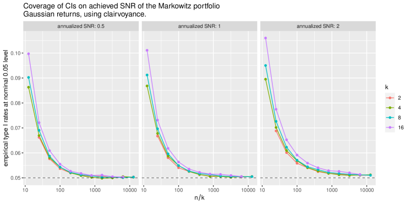
Figure 1: The empirical type I rate, over 1,000,000 simulations, of a one-sided confidence bound for $\zeta_{a}$ are shown for a nominal type I rate of $0.05$. The daily returns are drawn from multivariate normal distribution with varying ${\zeta}_{*}$, $n$, and $k$. Type I rates are plotted versus $n/k$ to indicate the requisite aspect ratio to achieve near nominal coverage.

In Figure 1 we plot the empirical type I rate at the nominal 0.05 level of the confidence bound. The main takeaway from this experiment is that the bound gives near-nominal coverage when $n\geq 100k$ or so.

2.1 Practical Inference

One can construct one- or two-sided confidence intervals from Inequality 10 when ${\zeta}_{*}$ is known. However, it is unknown in practice, and the constant ${{c}_{\alpha}}$ is sufficiently sensitive to it. To practically perform inference, there are two obvious routes: one is to jointly perform inference on ${\zeta}_{*}$ on ${\zeta}_{a}$; the other is to estimate ${\zeta}_{*}$ and plug it in when constructing ${{c}_{\alpha}}$.

For the joint estimation procedure, for some $q\in\left(0,1\right)$, construct a $q\alpha$ upper bound on ${\zeta}_{*}$. That confidence bound can be described implicitly via the connection to the non-central $F$ distribution: to find the one-sided confidence intervals $\left[0,{\zeta}_{u}\right]$ with coverage $1-q\alpha$, find

$${\zeta}_{u}=\min\left\{z\left|\;{z\geq 0,\,\,\alpha/2\geq{{F}_{f}}\left(\left(\frac{n(n-k)}{k(n-1)}\right){\hat{\zeta}}^{2}_{*};k,n-k,nz^{2}\right)}\right.\right\},$$ (13)

where ${{F}_{f}}\left(x;{{\nu}_{1}},{{\nu}_{2}},\delta\right)$ is the CDF of the non-central $F$-distribution with non-centrality parameter $\delta$ and ${{\nu}_{1}}$ and ${{\nu}_{2}}$ degrees of freedom. This method requires computational inversion of the CDF function. Then compute

$$c=\max\left\{\left.{{\chi^{2}}_{1-\left(1-q\right)\alpha}}\left(k,\frac{n\zeta^{2}}{4}\right)-\frac{n\zeta^{2}}{4}\right|0\leq\zeta\leq{\zeta}_{u}\right\}.$$

The bound ${\hat{\zeta}}_{*}-\frac{c}{n{\hat{\zeta}}_{*}}$ then should have type I rate at most $\alpha$. However, since this is a joint confidence bound the bound on ${\zeta}_{a}$ will be somewhat conservative.

Another approach, which does not have guaranteed coverage, is to estimate ${\zeta}_{*}$ from the data, and plug in that value in the computation of ${{c}_{\alpha}}$. We can perform this estimation using standard techniques, again via the connection of Hotelling’s $T^{2}$ to the $F$ distribution. Kubokawa, Robert and Saleh described improved methods for estimating the non-centrality parameter given an observation of a non-central $F$ statistic. [6]. They described the following estimators for the non-centrality parameter, which is ${\zeta}^{2}_{*}$ in our case:

$$\begin{split}\delta_{0}&=\frac{\left(n-k-2\right)}{n-1}{\hat{\zeta}}^{2}_{*}-\frac{k}{n},\\ \delta_{1}&=max\left(\delta_{0},0\right),\\ \delta_{2}&=max\left(\delta_{0},\frac{2}{k+2}\left(\delta_{0}+\frac{k}{n}\right)\right).\end{split}$$ (14)

They note that $\delta_{0}$ is the Uniform Minimum Variance Unbiased Estimator (UMVUE) of ${\zeta}^{2}_{*}$. However, it can be negative. The estimators $\delta_{1},\delta_{2}$ are non-negative, and dominate $\delta_{0}$ in having lower expected squared error. Thus the suggested procedure is to compute

$$c={{\chi^{2}}_{1-\alpha}}\left(k,\frac{n\delta_{2}}{4}\right)-\frac{n\delta_{2}}{4},$$

then use the bound ${\hat{\zeta}}_{*}-\frac{c}{n{\hat{\zeta}}_{*}}$. In practice this bound seems to give slightly less conservative coverage than the joint bound described above. It is not clear how to find a coverage guarantee for this bound. The quantities ${\hat{\zeta}}^{2}_{*}$ and ${\zeta}_{a}$ are not independent, and their asymptotic correlation is $\mathcal{O}\left(n^{-1/2}\right)$, which is only slowly shrinking. [9]

Feasible CI Coverage

We reconsider the experiments above but compute feasible confidence bounds. We use both the simultaneous CI approach with $q=0.25$; and plug in ${\zeta}_{*}=\sqrt{\delta_{2}}$ to construct the bound. In Figure 2, we plot the empirical type I rate for both of these bounds versus $n$, with facets for ${\zeta}_{*}$. We see that the $\delta_{2}$ plug-in estimator has coverage closer to the nominal $0.05$ rate. Both bounds have issues when $n/k$ is not sufficiently large, a problem stemming from the poor quality of the approximation $\mathsf{\hat{\Sigma}}\approx\mathsf{\hat{\Sigma}}$, and which was seen above. However, here we see closer to nominal coverage for larger $k$ for both methods. It is not clear how the coverage will behave for larger $n/k$, though that seems like an unlikely problem in practice.

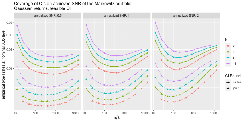
Figure 2: The empirical type I rate, over 1,000,000 simulations, of two feasible one-sided confidence bounds for $\zeta_{a}$ are shown for a nominal type I rate of $0.05$. The daily returns are drawn from multivariate normal distribution with varying ${\zeta}_{*}$, $n$, and $p$. The $y$ axis is drawn in square root scale to show detail.

2.2 Hedged Portfolios

Now we generalize the portfolio problem of Equation 1 to add a hedging constraint. So consider the constrained portfolio optimization problem on $k$ assets,

$$\max_{\begin{subarray}{c}\mathsf{G}\mathsf{\Sigma}\boldsymbol{\nu}=\boldsymbol{0},\\ {{\boldsymbol{\nu}}^{\top}}\mathsf{\Sigma}\boldsymbol{\nu}\leq R^{2}\end{subarray}}\frac{{{\boldsymbol{\nu}}^{\top}}\boldsymbol{\mu}-{{r}_{0}}}{\sqrt{{{\boldsymbol{\nu}}^{\top}}\mathsf{\Sigma}\boldsymbol{\nu}}},$$ (15)

where $\mathsf{G}$ is an ${{k}_{g}}\times k$ matrix of rank ${{k}_{g}}$, and, as previously, $\boldsymbol{\mu}$, $\mathsf{\Sigma}$ are the mean vector and covariance matrix, ${{r}_{0}}$ is the risk-free rate, and $R>0$ is a risk ‘budget’. We can interpret the $\mathsf{G}$ constraint as stating that the covariance of the returns of a feasible portfolio with the returns of a portfolio whose weights are in a given row of $\mathsf{G}$ shall equal zero. In the garden variety application of this problem, $\mathsf{G}$ consists of ${{k}_{g}}$ rows of the identity matrix; in this case, feasible portfolios are hedged with respect to the ${{k}_{g}}$ assets selected by $\mathsf{G}$ (although they may hold some position in the hedged assets). We use “hedged” to mean a portfolio with zero covariance against some other portfolio(s).

The solution to this problem, via the Lagrange multiplier technique, is

$${{\boldsymbol{\nu}}_{*,{\mathsf{I}}\setminus{\mathsf{G}}}}=c\left({{\mathsf{\Sigma}}^{-1}}{\boldsymbol{\mu}}-{{\mathsf{G}}^{\top}}{{\left(\mathsf{G}\mathsf{\Sigma}{{\mathsf{G}}^{\top}}\right)}^{-1}}\mathsf{G}\boldsymbol{\mu}\right).$$

When ${{r}_{0}}>0$, the unique solution is found by setting $c$ so that the risk budget is an equality. Note that, up to scaling, ${{\mathsf{\Sigma}}^{-1}}\boldsymbol{\mu}$ is the unconstrained optimal portfolio, and thus the imposition of the $\mathsf{G}$ constraint only changes the unconstrained portfolio in assets corresponding to columns of $\mathsf{G}$ containing non-zero elements. In the garden variety application where $\mathsf{G}$ is a single row of the identity matrix, the imposition of the constraint only changes the holdings in the asset to be hedged (modulo changes in the leading constant to satisfy the risk budget).

The squared signal-noise ratio of the optimal portfolio we write as

$${{\Delta}_{{\mathsf{I}}\setminus{\mathsf{G}}}}{\zeta}^{2}_{*}=_{\operatorname{df}}{{\boldsymbol{\mu}}^{\top}}{{\mathsf{\Sigma}}^{-1}}\boldsymbol{\mu}-{{\left(\mathsf{G}\boldsymbol{\mu}\right)}^{\top}}{{\left(\mathsf{G}\mathsf{\Sigma}{{\mathsf{G}}^{\top}}\right)}^{-1}}\left(\mathsf{G}\boldsymbol{\mu}\right).$$ (16)

The sample optimal portfolio is given by

$${{\boldsymbol{\hat{\nu}}}_{*,{\mathsf{I}}\setminus{\mathsf{G}}}}=c\left({{\mathsf{\hat{\Sigma}}}^{-1}}{\boldsymbol{\hat{\mu}}}-{{\mathsf{G}}^{\top}}{{\left(\mathsf{G}\mathsf{\hat{\Sigma}}{{\mathsf{G}}^{\top}}\right)}^{-1}}\mathsf{G}\boldsymbol{\hat{\mu}}\right).$$

The squared Sharpe ratio of this portfolio is

$${{\Delta}_{{\mathsf{I}}\setminus{\mathsf{G}}}}{\hat{\zeta}}^{2}_{*}={{\boldsymbol{\hat{\mu}}}^{\top}}{{\mathsf{\hat{\Sigma}}}^{-1}}\boldsymbol{\hat{\mu}}-{{\left(\mathsf{G}\boldsymbol{\hat{\mu}}\right)}^{\top}}{{\left(\mathsf{G}\mathsf{\hat{\Sigma}}{{\mathsf{G}}^{\top}}\right)}^{-1}}\left(\mathsf{G}\boldsymbol{\hat{\mu}}\right).$$ (17)

The achieved signal-noise ratio of this portfolio is

$${\zeta}_{a}=\frac{{{\boldsymbol{\mu}}^{\top}}{{\boldsymbol{\hat{\nu}}}_{*,{\mathsf{I}}\setminus{\mathsf{G}}}}}{\sqrt{{{{{\boldsymbol{\hat{\nu}}}_{*,{\mathsf{I}}\setminus{\mathsf{G}}}}}^{\top}}\mathsf{\Sigma}{{\boldsymbol{\hat{\nu}}}_{*,{\mathsf{I}}\setminus{\mathsf{G}}}}}}.$$ (18)

Define:

$${\hat{\zeta}}^{2}_{*,\mathsf{G}} =_{\operatorname{df}}{{\left(\mathsf{G}\boldsymbol{\hat{\mu}}\right)}^{\top}}{{\left(\mathsf{G}\mathsf{\hat{\Sigma}}{{\mathsf{G}}^{\top}}\right)}^{-1}}\left(\mathsf{G}\boldsymbol{\hat{\mu}}\right).$$

Giri showed that conditional on observing ${\hat{\zeta}}^{2}_{*,\mathsf{G}}$,

$$\frac{n}{n-1}\frac{n-k}{k-{{k}_{g}}}\frac{{{\Delta}_{{\mathsf{I}}\setminus{\mathsf{G}}}}{\hat{\zeta}}^{2}_{*}}{1+\frac{n}{n-1}{\hat{\zeta}}^{2}_{*,\mathsf{G}}}\left|\,{\hat{\zeta}}^{2}_{*,\mathsf{G}}\right.\sim F\left(k-{{k}_{g}},n-k,\frac{n}{1+\frac{n}{n-1}{\hat{\zeta}}^{2}_{*,\mathsf{G}}}{{\Delta}_{{\mathsf{I}}\setminus{\mathsf{G}}}}{\zeta}^{2}_{*}\right),$$ (19)

where $F\left({{v}_{1}},{{v}_{2}},\delta\right)$ is the non-central $F$-distribution with ${{v}_{1}}$, ${{v}_{2}}$ degrees of freedom and non-centrality parameter $\delta$. [giri1964likelihood, 11]

Now we apply Approximation 8, and complete the square as we did in the unhedged case, to find that

$${{\Delta}_{{\mathsf{I}}\setminus{\mathsf{G}}}}{\zeta}^{2}_{*}-{\zeta}_{a}\sqrt{{{\Delta}_{{\mathsf{I}}\setminus{\mathsf{G}}}}{\zeta}^{2}_{*}} \approx{{\left(\boldsymbol{\hat{\mu}}-\boldsymbol{\mu}\right)}^{\top}}{{\mathsf{\Sigma}}^{-1}}\boldsymbol{\hat{\mu}}-{{\left(\boldsymbol{\hat{\mu}}-\boldsymbol{\mu}\right)}^{\top}}{{\mathsf{G}}^{\top}}{{\left(\mathsf{G}\mathsf{\Sigma}{{\mathsf{G}}^{\top}}\right)}^{-1}}\mathsf{G}\boldsymbol{\hat{\mu}},$$

$$=\frac{1}{n}\left[{{\left(\frac{1}{2}\sqrt{n}{{\mathsf{\Sigma}}^{-1/2}}\boldsymbol{\mu}+\boldsymbol{z}\right)}^{\top}}\left(\mathsf{I}-{{\mathsf{\Sigma}}^{\top/2}}{{\mathsf{G}}^{\top}}{{\left(\mathsf{G}\mathsf{\Sigma}{{\mathsf{G}}^{\top}}\right)}^{-1}}\mathsf{G}{{\mathsf{\Sigma}}^{1/2}}\right)\left(\frac{1}{2}\sqrt{n}{{\mathsf{\Sigma}}^{-1/2}}\boldsymbol{\mu}+\boldsymbol{z}\right)\right]$$

$$\phantom{=}\,-\frac{1}{4n}\left[{{\left(\sqrt{n}{{\mathsf{\Sigma}}^{-1/2}}\boldsymbol{\mu}\right)}^{\top}}\left(\mathsf{I}-{{\mathsf{\Sigma}}^{\top/2}}{{\mathsf{G}}^{\top}}{{\left(\mathsf{G}\mathsf{\Sigma}{{\mathsf{G}}^{\top}}\right)}^{-1}}\mathsf{G}{{\mathsf{\Sigma}}^{1/2}}\right)\left(\sqrt{n}{{\mathsf{\Sigma}}^{-1/2}}\boldsymbol{\mu}\right)\right],$$

where $\boldsymbol{z}\sim\mathcal{N}\left(\boldsymbol{0},\mathsf{I}\right).$ Now note that the matrix

$$\mathsf{A}={\mathsf{I}-{{\mathsf{\Sigma}}^{\top/2}}{{\mathsf{G}}^{\top}}{{\left(\mathsf{G}\mathsf{\Sigma}{{\mathsf{G}}^{\top}}\right)}^{-1}}\mathsf{G}{{\mathsf{\Sigma}}^{1/2}}}$$

is idempotent with rank $k-{{k}_{g}}$. Thus a quadratic form in $\mathsf{A}$ follows a non-central $\chi^{2}$ distribution with degrees of freedom equal to the rank of $\mathsf{A}$. [10.2307/2237227, Theorem 2] Thus

$${{\Delta}_{{\mathsf{I}}\setminus{\mathsf{G}}}}{\zeta}^{2}_{*}-{\zeta}_{a}\sqrt{{{\Delta}_{{\mathsf{I}}\setminus{\mathsf{G}}}}{\zeta}^{2}_{*}}\sim\frac{1}{n}\left(\chi^{2}\left(k-{{k}_{g}},\frac{n{{\Delta}_{{\mathsf{I}}\setminus{\mathsf{G}}}}{\zeta}^{2}_{*}}{4}\right)-\frac{n{{\Delta}_{{\mathsf{I}}\setminus{\mathsf{G}}}}{\zeta}^{2}_{*}}{4}\right).$$

Then, as in the unhedged case, we have

$$\operatorname{Pr}\left\{{\zeta}_{a}\leq\sqrt{{{\Delta}_{{\mathsf{I}}\setminus{\mathsf{G}}}}{\hat{\zeta}}^{2}_{*}}-\frac{{{c}_{\alpha}}}{n\sqrt{{{\Delta}_{{\mathsf{I}}\setminus{\mathsf{G}}}}{\hat{\zeta}}^{2}_{*}}}\right\}=\alpha,$$ (20)

if we let

$${{c}_{\alpha}}={{{\chi^{2}}_{1-\alpha}}\left(k-{{k}_{g}},\frac{n{{\Delta}_{{\mathsf{I}}\setminus{\mathsf{G}}}}{\zeta}^{2}_{*}}{4}\right)-\frac{n{{\Delta}_{{\mathsf{I}}\setminus{\mathsf{G}}}}{\zeta}^{2}_{*}}{4}}.$$

To perform feasible inference one will need to estimate ${{\Delta}_{{\mathsf{I}}\setminus{\mathsf{G}}}}$ ${\zeta}^{2}_{*}$. Again this will be via the connection to a non-central $F$-distribution, Equation 19. One can either find an upper quantile directly, or use a KRS-type estimator, which for the hedged case are

$$\begin{split}\delta_{0}&=\frac{\left(n-k-2\right)}{n-1}{{\Delta}_{{\mathsf{I}}\setminus{\mathsf{G}}}}{\hat{\zeta}}^{2}_{*}-\frac{k-{{k}_{g}}}{n}\left(1+\frac{n}{n-1}{\hat{\zeta}}^{2}_{*,\mathsf{G}}\right),\\ \delta_{1}&=max\left(\delta_{0},0\right),\\ \delta_{2}&=max\left(\delta_{0},\frac{2}{k-{{k}_{g}}+2}\frac{n-k-2}{n-1}{{\Delta}_{{\mathsf{I}}\setminus{\mathsf{G}}}}{\hat{\zeta}}^{2}_{*}\right).\end{split}$$ (21)

Checking coverage

As in the unhedged case, we first perform simulations where the population parameter ${{\Delta}_{{\mathsf{I}}\setminus{\mathsf{G}}}}$ ${\zeta}^{2}_{*}$ is known, to assess the effects of Approximation 8. In our simulations, we set ${{k}_{g}}=k/2$, and let $\mathsf{G}$ be the first ${{k}_{g}}$ rows of the identity matrix. We set $\boldsymbol{\mu}=c\boldsymbol{1}$ and $\mathsf{\Sigma}=\mathsf{I}$. We perform $100,000$ simulations for different values of ${{\Delta}_{{\mathsf{I}}\setminus{\mathsf{G}}}}{\zeta}^{2}_{*}$, $k$ and $n$, computing ${\zeta}_{a}$ for the hedged portfolio, as well as ${{\Delta}_{{\mathsf{I}}\setminus{\mathsf{G}}}}$ ${\hat{\zeta}}^{2}_{*}$ and ${\hat{\zeta}}^{2}_{*,\mathsf{G}}$. We compute the lower 0.05 bound using knowledge of ${{\Delta}_{{\mathsf{I}}\setminus{\mathsf{G}}}}$ ${\zeta}^{2}_{*}$ and compute the empirical type I rate over the $100,000$ simulations, which we plot versus $n/k$ in Figure 3. Again we see that the nominal type I rate is nearly achieved when $n>100k$ or so.

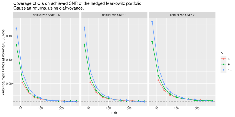
Figure 3: The empirical type I rate, over 100,000 simulations, of a one-sided confidence bound for $\zeta_{a}$ are shown for the hedged portfolio problem. We set ${{k}_{g}}=k/2$ and take $\boldsymbol{\mu}\propto\boldsymbol{1}$. The SNR in the facet titles refers to $\sqrt{{{\Delta}_{{\mathsf{I}}\setminus{\mathsf{G}}}}{\zeta}^{2}_{*}}$.

As above we analyze the data from the hedged experiments, but compute feasible confidence bounds. We use both the simultaneous CI approach with $q=0.25$; and plug in ${{\Delta}_{{\mathsf{I}}\setminus{\mathsf{G}}}}{\zeta}^{2}_{*}=\sqrt{\delta_{2}}$ to construct the bound. In Figure 4, we plot the empirical type I rate for both of these bounds versus $n$, with facets for ${\zeta}_{*}$ and $k$. Once again, the $\delta_{2}$ plug-in estimator has coverage closer to the nominal $0.05$ rate, and both bounds are anti-conservative when $n/k$ is not sufficiently large.

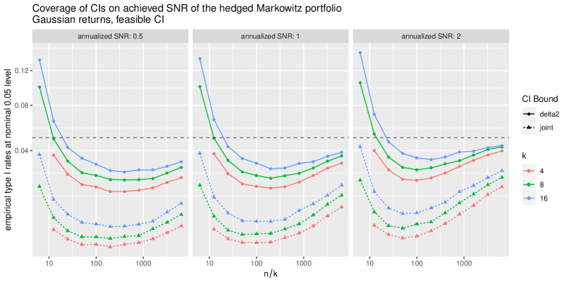
Figure 4: The empirical type I rate, over 100,000 simulations, of two feasible one-sided confidence bounds for $\zeta_{a}$ are shown for a nominal type I rate of $0.05$. The daily returns are drawn from multivariate normal distribution with varying ${\zeta}_{*}$, $n$, and $p$. The $y$ axis is drawn in square root scale to show detail.

3 Examples

Fama French 4 Factor Returns

We consider a portfolio constructed on the ‘Market’, size (SMB), value (HML) and momentum (HMD) portfolios described by Fama and French, inter alia, with data compiled and published by Kenneth French. [4, 3, 5] The set consists of $n=1104\,\mbox{mo.}$ of data, from 1927 through 2018.917. We observe ${\hat{\zeta}}^{2}_{*}=0.098\,{{\mbox{mo.}}^{-1}}$. From this we compute $\delta_{2}=0.094\,{{\mbox{mo.}}^{-1}}$. Plugging in $\sqrt{\delta_{2}}$ for ${\zeta}_{*}$ we compute a two-sided $95\%$ confidence bound on ${\zeta}_{a}$ as $\left[0.234,0.353\right]\,{{\mbox{mo.}}^{-1/2}}$. By comparison, via the connection to the $F$ distribution, we compute $95\%$ confidence intervals on ${\zeta}_{*}$ as $\left[0.247,0.369\right]\,{{\mbox{mo.}}^{-1/2}}$.

Next we consider the imposition of a constraint that the portfolio should be “hedged against the Market”. This corresponds to ${{k}_{g}}=1$ and $\mathsf{G}$ is the row of the identity matrix corresponding to the Market factor. We compute

$${\hat{\zeta}}^{2}_{*}=0.098\,{{\mbox{mo.}}^{-1}},\quad{\hat{\zeta}}^{2}_{*,\mathsf{G}}=0.03\,{{\mbox{mo.}}^{-1}},\quad{{\Delta}_{{\mathsf{I}}\setminus{\mathsf{G}}}}{\hat{\zeta}}^{2}_{*}=0.068\,{{\mbox{mo.}}^{-1}}.$$

With $n=1104,k=4$, we compute the three KRS estimators of ${{\Delta}_{{\mathsf{I}}\setminus{\mathsf{G}}}}$ ${\zeta}^{2}_{*}$, which all take the same value, $\delta_{0}=\delta_{1}=\delta_{2}=0.065{{\mbox{mo.}}^{-1}}.$ From this we compute a one-sided $95\%$ confidence bound on ${\zeta}_{a}$ to be $\left[0.195,\infty\right)\,{{\mbox{mo.}}^{-1/2}}$.

4 Discussion

Testing indicates the confidence bound exhibits closer to nominal coverage than the known asymptotic bounds for reasonable $n$ and $k$. Further work should naturally focus on mitigating the effects of the approximation $\mathsf{\hat{\Sigma}}\approx\mathsf{\Sigma}$, and finding a coverage guarantee of the plug-in estimator. We also anticipate that this confidence bound procedure can be adapted to deal with conditional expectation models.

References

Anderson [2003]
T. W. Anderson.
An Introduction to Multivariate Statistical Analysis.
Wiley Series in Probability and Statistics. Wiley, 2003.
ISBN 9780471360919.
URL http://books.google.com/books?id=Cmm9QgAACAAJ.
Carhart [1997]
Mark M Carhart.
On persistence in mutual fund performance.
Journal of Finance, 52(1):57, 1997.
URL http://www.jstor.org/stable/2329556.
Fama and French [1992]
Eugene F. Fama and Kenneth R. French.
The cross-section of expected stock returns.
Journal of Finance, 47(2):427, 1992.
URL http://www.jstor.org/stable/2329112.
Kubokawa et al. [1993]
Tatsuya Kubokawa, C. P. Robert, and A. K. Md. E. Saleh.
Estimation of noncentrality parameters.
Canadian Journal of Statistics, 21(1):45–57, Mar 1993.
URL http://www.jstor.org/stable/3315657.
Paulsen and Söhl [2020]
Dirk Paulsen and Jakob Söhl.
Noise fit, estimation error and a Sharpe information criterion.
Quantitative Finance, 0(0):1–17, 2020.
doi: 10.1080/14697688.2020.1718746.
URL https://doi.org/10.1080/14697688.2020.1718746.
Pav [2013]
Steven E. Pav.
Asymptotic distribution of the Markowitz portfolio.
Privately Published, 2013.
URL http://arxiv.org/abs/1312.0557.