Exponential stability for time-delay neural networks via new weighted integral inequalities

Abstract

We study exponential stability for a kind of neural networks having time-varying delay. By extending the auxiliary function-based integral inequality, a novel integral inequality is derived by using weighted orthogonal functions of which one is discontinuous. Then, the new inequality is applied to investigate the exponential stability of time-delay neural networks via Lyapunov-Krasovskii functional (LKF) method. Numerical examples are given to verify the advantages of the proposed criterion.

Key words: Neural networks; exponential stability; Lyapunov-Krasovskii functional; time-varying delay.

1 Introduction

With the development of new scientific technology, neural networks have been adopted to different applications such as image decryption, pattern recognition, and finance [1, 2, 3, 4, 5]. In general, a practical neural network involves a lot of neurons to perform several complex tasks. As it was particularly pointed out in [6], time delays of information exchange between these large number of neurons are unavoidable. At the same time, a delay term in a system, even though it may not be large, is usually a key factor to cause a neural network unstable. Therefore, the problem of studying the effect of time delay plays a critical role in the study of neural networks and this issue has been extensively studied in recent years[7, 8].

As we know, it is an important task to make stability criteria less conservative when analyzing time-delay systems [9, 10, 11, 12, 13]. More specifically, exponential stability is desirable for some applications[14, 15, 16, 17]. To this end, various approaches have been developed to the subject, which include techniques of free weighting matrices [18], reciprocally convex optimization [19] and delay-partitioning [20, 21]. Exponential stability analysis of time-delay neural networks aims at deriving an admissible delay upper bound (ADUB) such that the delayed neural networks are stable for all time-delays less than the obtained ADUB. Roughly speaking, ADUB measures the conservatism of a stability criterion. If a stability criterion can yield a larger or sharper ADUB than another one, the criterion is less conservative. It is shown in [22] that the LKF method plus linear matrix inequality (LMI) technique is useful to determining the ADUB for delayed systems.

Until now, a great number of integral inequalities have been proposed to study delayed systems, such as the Wirtinger-based inequality [16, 17], the Bessel-Legendre inequality [23, 24, 25] and the auxiliary function-based inequalities [26, 27]. In this paper, we study the auxiliary function-based inequality which was developed for the theoretical study of the delayed systems in [28]. Since it gives tighter estimates than the Jensen inequality, compared with the extend form of Jensen inequality [29, 30], employing this inequality can yield less conservative asymptotic stability criteria for some delayed systems. Based on [28], a further improved integral inequality was established in [27] by considering a group of orthogonal functions of which one is discontinuous. Instead of using high-degree polynomial to sharpen the bound, a discontinuous function is employed to reduce the number of decision variables (NODVs).

In the current study, we aim to investigate the exponential stability of neural networks having time-varying delay following ideas in [28, 27]. Different from [27], basing on our previous study [31], we considered the orthogonal sets $\{p_{0}({\cdot}),\ \ p_{1}(\cdot),\ \ p_{2}(\cdot)\}$ with respect to an exponential term, which is called a weight function. By combining the decomposition of the state vectors, which consists of polynomials, and $\{p_{0}(\cdot),\ \ p_{2}(\cdot),\ \ p_{3}(\cdot)\}$, where $p_{3}(\cdot)$ is a discontinuous function, a novel weighted inequality is established. Our new weighted inequality was derived by improving the one in [27] and estimating integrals with exponential term as a whole. An improved criterion which guarantees exponential stability of neural networks having time-varying delay is derived by using our new inequality. Numerical examples are given to confirm the advantage of the method proposed in this paper.

The following points outline the main contributions of this paper:

• A new weighted inequality, which generalizes the integral inequality based on auxiliary function in [28], is established. The inequality can be used to establish an improved exponential stability criterion for delayed systems.

• We consider time-varying delay which is not necessary nondecreasing (noting that nondecreasing was assumed in the proof of [27]). By further studying the LKF in [27], we find that some terms in the LKF can be removed to reduce the number of decision variables in the stability criterion without affecting its performance.

We organize our paper as follows. The model of neural networks with time-varying delay and the new weighted inequality are introduced in Section 2. By using a refined LKF, our main theoretial result is given in Section 3. For the last section, simulations are carried out to demonstrate the proposed criterion.

Notations: We use $\mathbb{R}^{n}$ and $\mathbb{R}^{n\times m}$ are the sets of $m$-dimensional Euclidean vector space and $n\times m$ real matrix space. When a real matrix $P$ is symmetric and positive definite (semi-positive definite), we describe this using $P>0~{}(\geq 0)$. The notation ${\rm diag}\{\cdots\}$ refers to a diagonal matrix. Additionally, we take $\mathbb{S}_{n}^{+}$ as the set of symmetric positive definite matrices and symmetric terms in a symmetric matrix are marked as $*$ for simplicity of presentation. Finally, we define $sym(A)=A+A^{T}$, where $T$ represents transpose of a matrix

2 Preliminaries

We study time-delay neural networks as follow

$$\dot{x}(t)=-Cx(t)+Ag(x(t))+Bg(x(t-h(t)))+u,$$ (2.1)

where the neuron state vector is denoted by $x(\cdot)=[x_{1}(\cdot),x_{2}(\cdot),\ldots,x_{n}(\cdot)]^{T}\in\mathbb{R}^{n}$ and the activation function is $g(x(\cdot))=[g_{1}(x_{1}(\cdot)),g_{2}(x_{2}(\cdot)),\ldots,g_{n}(x_{n}(\cdot))]^{T}\in\mathbb{R}^{n}$ . The vector $u=[u_{1},u_{2},\ldots,u_{n}]^{T}\in\mathbb{R}^{n}$ is an input to the network. Entries of the matrix $C=\emph{diag}\{c_{1},c_{2},\ldots,c_{n}\}$ satisfy $c_{i}>0$. The matrices $A$ and $B$ are weight matrices corresponding to connection. The differentiable function $h(t)$ denotes the time-varying delay and it holds that

$$0\leq h(t)\leq h$$ (2.2)

and

$${|\dot{h}(t)|}\leq\mu$$ (2.3)

for some constants $\mu$ and $h$. As in previous studies, we assumed that each activation function of (2.1) satisfies:

$$0\leq\frac{g_{j}(x)-g_{i}(y)}{x-y}\leq L_{j},\quad x,y\in\mathbb{R},\quad x\neq y,\quad j=1,2,\ldots,n,$$ (2.4)

for some positive constants $L_{j},~{}j=1,2,\ldots,n$.
Under (2.4), there exists an $x^{*}=[x^{*}_{1},x^{*}_{2},\ldots,x^{*}_{n}]^{T}$ such that

$$Cx^{*}=Ag(x^{*})+Bg(x^{*})+u.$$ (2.5)

Then shift the the equilibrium point $x^{*}$ of system (2.1) to the origin by the transform $z(\cdot)=x(\cdot)-x^{*}$. Then $z=[z_{1}(\cdot),z_{2}(\cdot),\ldots,z_{n}(\cdot)]^{T}$ satisfies

$$\dot{z}(t)=-Cz(t)+Af(z(t))+Bf(z(t-h(t)))$$ (2.6)

where $f(z(\cdot))=[f_{1}(z_{1}(\cdot)),f_{2}(z_{2}(\cdot)),\ldots,f_{n}(z_{n}(\cdot))]^{T}$ and $f_{j}(z_{j}(\cdot))=g_{j}(z_{j}(\cdot)+x^{*}_{j})-g_{j}(x_{j}^{*}),j=1,2,\ldots,n$. With these notations, we have

$$0\leq\frac{f_{j}(z_{j})}{z_{j}}\leq L_{j},\quad f_{j}(0)=0,\quad\forall z_{j}\neq 0,\quad j=1,2,\ldots,n.$$ (2.7)

Definition of exponential stability of (2.6) is given below.

Definition 2.1.

[27] The neural network (2.6) is exponentially stable at the origin if, for $t>0$,

$$\|z(t)\|\,\leq H\phi e^{-kt}$$

holds for some positive constants $k>0$ and $H\geq 1$, where $\phi=sup_{-h\leq\theta\leq 0}\|z(\theta)\|\,$. In this situation, we call $k$ the exponential convergence rate.

The well-known reciprocally convex inequality are useful for the theoretical proof and it is summarized as below:

Lemma 2.2.

[32] Suppose that $f_{1},f_{2},\ldots,f_{n}:\mathbb{R}^{m}\rightarrow\mathbb{R}$ take positive values in an open subsets $D$ of $\mathbb{R}^{m}$ then the below equation holds:

$$\min\limits_{\Big{\{}\alpha_{i}\mid\alpha_{i}>0,\sum\limits_{i}a_{i}=1\Big{\}}}\sum\limits_{i}\frac{1}{\alpha_{i}}f_{i}(t)=\sum\limits_{i}f_{i}(t)+\max_{g_{ij}(t)}\sum\limits_{i\neq j}g_{ij}(t)$$ (2.8)

subject to

$$\Bigg{\{}g_{ij}:\mathbb{R}^{m}\rightarrow\mathbb{R},g_{ji}\triangleq g_{ij},\left[\begin{array}[]{ccc}f_{i}(t)&g_{ij}(t)\\ g_{ji}(t)&f_{j}(t)\\ \end{array}\right]\geq 0\Bigg{\}}$$

In the following, some new weighted integral inequalities are derived by refining those established in [27] and [31]. Let $p_{i}(u)$ for $i=0,1,2,3$ be some scalar functions on $[a,b]$ and the weight function $w(u)$ is large than zero. Considering a product between two functions as follow

$$\langle p_{i},p_{j}\rangle=\int_{a}^{b}p_{i}(u)p_{j}(u)w(u)du$$

and functions $\{p_{0},p_{1},p_{2},p_{3}\}$ satisfying the “orthogonal” properties as follow:

$$\int_{a}^{b}p_{0}(u)p_{i}(u)w(u)du=0\,\,(i=1,2,3),\,\,\int_{a}^{b}p_{1}(u)p_{2}(u)w(u)du=0,\,\,\int_{a}^{b}p_{2}(u)p_{3}(u)w(u)du=0.$$ (2.9)

In particular, we take $p_{0}(u)\equiv 1$. The main estimate in this paper read as:

Lemma 2.3.

For a matrix $R\in\mathbb{S}_{n}^{+}$, we have

$$\int_{a}^{b}\phi^{T}(u)R\phi(u)w(u)du \geq \frac{1}{q_{0}}F_{0}^{T}RF_{0}+\frac{1}{q_{1}}F_{1}^{T}RF_{1}+\frac{1}{q_{2}}F_{2}^{T}RF_{2}$$ (2.10)

$$+\frac{1}{q_{3}}\biggr{[}F_{3}-\frac{q_{13}}{q_{1}}F_{1}\biggr{]}^{T}R\biggr{[}F_{3}-\frac{q_{13}}{q_{1}}F_{1}\biggr{]}$$

where

$$F_{i}=\int_{a}^{b}p_{i}(u)\phi_{i}(u)w(u)du,\quad q_{i}=\int_{a}^{b}p_{i}^{2}(u)w(u)du,\quad i=0,1,2,3,$$

$$F_{0}=\int_{a}^{b}\phi(u)w(u)du,\quad q_{0}=\int_{a}^{b}w(u)du,\quad q_{13}=\int_{a}^{b}p_{1}(u)p_{3}(u)w(u)du$$

Proof.

Let

$$e(u)=\phi(u)-\frac{F_{0}}{q_{0}}-\frac{F_{1}}{q_{1}}p_{1}(u)-\frac{F_{2}}{q_{2}}p_{2}(u)-p_{3}(u)v$$

where $v$ is a constant vector in $\mathbb{R}^{n}$. Since $R$ is positive definite, if we take

$$v=\frac{F_{3}}{q_{3}}-\frac{\int_{a}^{b}p_{1}(u)p_{3}(u)w(u)du}{q_{1}q_{3}}F_{1},$$

we have

$$\int_{a}^{b} e^{T}(u)Re(u)w(u)du$$

$$= \int_{a}^{b}\biggr{[}\phi(u)-\frac{F_{0}}{q_{0}}-\frac{F_{1}}{q_{1}}p_{1}(u)-\frac{F_{2}}{q_{2}}p_{2}(u)-p_{3}(u)v\biggr{]}^{T}R\biggr{[}\phi(u)-\frac{F_{0}}{q_{0}}$$

$$-\frac{F_{1}}{q_{1}}p_{1}(u)-\frac{F_{2}}{q_{2}}p_{2}(u)-p_{3}(u)v\biggr{]}w(u)du$$

$$= \int_{a}^{b}\biggr{[}\phi(u)-\frac{F_{0}}{q_{0}}-\frac{F_{1}}{q_{1}}p_{1}(u)-\frac{F_{2}}{q_{2}}p_{2}(u)\biggr{]}^{T}R\biggr{[}\phi(u)-\frac{F_{0}}{q_{0}}-\frac{F_{1}}{q_{1}}p_{1}(u)-\frac{F_{2}}{q_{2}}p_{2}(u)\biggr{]}w(u)du$$

$$-2\int_{a}^{b}\biggr{[}\phi(u)p_{3}(u)-\frac{F_{0}}{q_{0}}p_{3}(u)-\frac{F_{1}}{q_{1}}p_{1}(u)p_{3}(u)-\frac{F_{2}}{q_{2}}p_{2}(u)p_{3}(u)\biggr{]}^{T}w(u)duRv$$

$$+\int_{a}^{b}p_{3}^{2}(u)w(u)duv^{T}Rv$$

$$= \int_{a}^{b}\biggr{[}\phi(u)-\frac{F_{0}}{q_{0}}-\frac{F_{1}}{q_{1}}p_{1}(u)-\frac{F_{2}}{q_{2}}p_{2}(u)\biggr{]}^{T}R\biggr{[}\phi(u)-\frac{F_{0}}{q_{0}}-\frac{F_{1}}{q_{1}}p_{1}(u)-\frac{F_{2}}{q_{2}}p_{2}(u)\biggr{]}w(u)du-q_{3}v^{T}Rv$$

$$= \int_{a}^{b}\phi^{T}(u)R\phi(u)w(u)du-2\int_{a}^{b}\phi^{T}(u)R\biggr{[}\frac{F_{0}}{q_{0}}+\frac{F_{1}}{q_{1}}p_{1}(u)+\frac{F_{2}}{q_{2}}p_{2}(u)\biggr{]}w(u)du$$

$$+\int_{a}^{b}\biggr{[}\frac{F_{0}}{q_{0}}+\frac{F_{1}}{q_{1}}p_{1}(u)+\frac{F_{2}}{q_{2}}p_{2}(u)\biggr{]}^{T}R\biggr{[}\frac{F_{0}}{q_{0}}+\frac{F_{1}}{q_{1}}p_{1}(u)+\frac{F_{2}}{q_{2}}p_{2}(u)\biggr{]}w(u)du-q_{3}v^{T}Rv$$

$$= \int_{a}^{b}\phi^{T}(u)R\phi(u)w(u)du-\frac{1}{q_{0}}F_{0}^{T}RF_{0}-\frac{1}{q_{1}}F_{1}^{T}RF_{1}-\frac{1}{q_{2}}F_{2}^{T}RF_{2}-q_{3}v^{T}Rv\geq 0,$$

which is equivalent to

$$\int_{a}^{b}\phi^{T}(u)R\phi(u)w(u)du\geq\frac{1}{q_{0}}F_{0}^{T}RF_{0}+\frac{1}{q_{1}}F_{1}^{T}RF_{1}+\frac{1}{q_{2}}F_{2}^{T}RF_{2}+\frac{1}{q_{3}}\biggr{[}F_{3}-\frac{q_{13}}{q_{1}}F_{1}\biggr{]}^{T}R\biggr{[}F_{3}-\frac{q_{13}}{q_{1}}F_{1}\biggr{]}.$$

∎

Consider the weight function $w(u)=e^{-2k(u-b)}$ and $\phi(u)=e^{2k(u-b)}z(u)$ in (2.10). We can get the following inequality:

Lemma 2.4.

Consider an integrable function $z:[a,b]\rightarrow\mathbb{R}^{n}$ and a matrix $R\in\mathbb{S}_{n}^{+}$. We have the following inequality:

$$\int_{a}^{b}e^{2k(u-b)}z^{T}(u)Rz(u)du \geq \frac{1}{q_{0}}\Omega_{0}^{T}R\Omega_{0}+\frac{1}{q_{1}}\Omega_{1}^{T}R\Omega_{1}+\frac{1}{q_{2}}\Omega_{2}^{T}R\Omega_{2}$$ (2.11)

$$+\frac{1}{q_{3}}\biggr{[}\Omega_{3}-\frac{q_{13}}{q_{1}}\Omega_{1}\biggr{]}^{T}R\biggr{[}\Omega_{3}-\frac{q_{13}}{q_{1}}\Omega_{1}\biggr{]}$$

where

$$\Omega_{0} = \int_{a}^{b}z(u)du,\ \ \ \Omega_{1}=c_{1}\int_{a}^{b}z(u)du+\int_{a}^{b}\int_{s}^{b}z(u)duds,$$

$$\Omega_{2} = c_{3}\int_{a}^{b}z(u)du+c_{2}\int_{a}^{b}\int_{s}^{b}z(u)duds+2\int_{a}^{b}\int_{s}^{b}\int_{u}^{b}z(v)dvduds,$$

$$\Omega_{3} = \int_{a}^{b}z(u)du+c_{4}\int_{a}^{\xi}z(u)du,\ \ \ w=e^{2k(b-a)},\ \ \ c_{1}=\frac{b-a}{w-1}-\frac{1}{2k},$$

$$c_{2} = {-\frac{\frac{(w-1)}{2k^{3}}-(b-a)^{3}-\frac{(b-a)^{2}}{k}-\frac{(b-a)}{2k^{2}}-\frac{(b-a)^{3}}{w-1}-\frac{(b-a)^{2}}{k(w-1)}}{\frac{w-1}{4k^{2}}-(b-a)^{2}-\frac{(b-a)^{2}}{w-1}}}$$

$$c_{3} = c_{1}c_{2}-(\frac{1}{2k^{2}}-\frac{(b-a)^{2}}{w-1}-\frac{(b-a)}{k(w-1)}),\ \ \ c_{4}=-\frac{w-1}{w-e^{-2k(\xi-b)}},$$

$$q_{0} = \frac{w-1}{2k},\ \ \ q_{1}={\frac{w-1}{8k^{3}}-\frac{(b-a)^{2}}{2k}-\frac{(b-a)^{2}}{2k(w-1)}},$$

$$q_{2} = {\frac{3(w-1)}{4k^{5}}-\frac{(b-a)^{4}}{2k}-\frac{(b-a)^{3}}{k^{2}}-\frac{3(b-a)^{2}}{2k^{3}}-\frac{3(b-a)}{2k^{4}}-c_{2}^{2}q_{1}-(c_{3}-c_{1}c_{2})^{2}q_{0}.}$$

$$q_{3} = {(\frac{w-1}{2k})(\frac{e^{-2k(\xi-b)}-1}{w-e^{-2k(\xi-b)}})},\ \ \ q_{13}=\frac{(w-1)(\xi-a)e^{-2k(\xi-b)}}{2k(w-e^{-2k(\xi-b)})}-\frac{b-a}{2k}.$$

Proof.

In order to use Lemma 2.3, we first introduce the function $p_{3}$. Noting that $p_{3}$ can be a discontinuous function and it must satisfy $\langle p_{3},1\rangle=\langle p_{3},p_{2}\rangle=0$ and $\langle p_{3},p_{1}\rangle\neq 0$. Let $\xi\in(a,b)$ be such that $\int_{a}^{\xi}p_{2}(u)w(u)dt=0$ and denote $p_{3}=1-\frac{\langle 1,1\rangle}{\langle 1,\chi\rangle}\chi$, where $\chi(u)=\left\{\begin{array}[]{ll}1&\textrm{if $u\in[a,\xi]$}\\ 0&\textrm{if $u\in(\xi,b]$}\end{array}\right.$. We can get $\langle p_{3},p_{2}\rangle=\langle 1,p_{2}\rangle-\frac{\langle 1,1\rangle}{\langle 1,\chi\rangle}\langle\chi,p_{2}\rangle=0$ and $\langle p_{3},1\rangle=\langle 1,1\rangle-\frac{\langle 1,1\rangle}{\langle 1,\chi\rangle}\langle\chi,1\rangle=0$.

Then we take $p_{1}(u),~{}p_{2}(u)$ as linear and quadratic polynomial:

$$p_{1}(u)=(u-a)+c_{1},\ \ \ p_{2}(u)=(u-a)^{2}+c_{2}(u-a)+c_{3}.$$

which satisfied $\int_{a}^{b}p_{i}(u)w(u)du=0\ \ (i=1,2)$ and $\int_{a}^{b}p_{1}(u)p_{2}(u)w(u)du=0$. We can get $c_{1}=-\frac{\int_{a}^{b}(u-a)w(u)du}{\int_{a}^{b}w(u)du}$, $c_{2}=-\frac{\int_{a}^{b}(u-a)^{2}p_{1}(u)w(u)du}{\int_{a}^{b}p_{1}(u)p_{1}(u)w(u)du}$, $c_{3}=c_{2}c_{1}-\frac{\int_{a}^{b}(u-a)^{2}w(u)du}{\int_{a}^{b}w(u)du}$ by simple calculations.

Denote $c_{4}=-\frac{\langle 1,1\rangle}{\langle 1,\chi\rangle}$, then straight computations leads to

$$F_{0} =\int_{a}^{b}\phi(u)w(u)du=\int_{a}^{b}z(u)du=\Omega_{0},$$

$$F_{1} =\int_{a}^{b}p_{1}(u)\phi(u)w(u)du=c_{1}\int_{a}^{b}z(u)du+\int_{a}^{b}\int_{s}^{b}z(u)duds=\Omega_{1},$$

$$F_{2} =\int_{a}^{b}p_{2}(u)\phi(u)w(u)du=c_{3}\int_{a}^{b}z(u)du+c_{2}\int_{a}^{b}\int_{s}^{b}z(u)duds+2\int_{a}^{b}\int_{s}^{b}\int_{u}^{b}z(v)dvduds=\Omega_{2},$$

$$F_{3} =\int_{a}^{b}p_{3}(u)\phi(u)w(u)du=\int_{a}^{b}z(u)du+c_{4}\int_{a}^{\xi}z(u)du=\Omega_{3}.$$

By Lemma 2.3, the inequality (2.11) holds.

∎

Particularly, when $w(u)=1$, we have the following lemma.

Lemma 2.5.

[27] Given an integrable function $z$ $:[a,b]\rightarrow\mathbb{R}^{n}$ and a matrix $R\in\mathbb{S}_{n}^{+}$, one has following:

$$\int_{a}^{b}z^{T}(u)Rz(u)du \geq \frac{1}{b-a}\omega_{0}^{T}R\omega_{0}+\frac{3}{b-a}\omega_{1}^{T}R\omega_{1}+\frac{5}{b-a}\omega_{2}^{T}R\omega_{2}$$ (2.12)

$$+\frac{1}{b-a}\biggr{[}\omega_{3}-\frac{3}{2}\omega_{1}\biggr{]}^{T}R\biggr{[}\omega_{3}-\frac{3}{2}\omega_{1}\biggr{]}$$

where

$$\omega_{0} = \int_{a}^{b}z(u)du,$$

$$\omega_{1} = \int_{a}^{b}z(u)du-\frac{2}{b-a}\int_{a}^{b}\int_{s}^{b}z(u)duds,$$

$$\omega_{2} = \int_{a}^{b}z(u)du-\frac{6}{b-a}\int_{a}^{b}\int_{s}^{b}z(u)duds+\frac{12}{(b-a)^{2}}\int_{a}^{b}\int_{s}^{b}\int_{v}^{b}z(u)dudvds,$$

$$\omega_{3} = \int_{a}^{\frac{a+b}{2}}z(u)du-\int_{\frac{a+b}{2}}^{b}z(u)du.$$

Remark 2.6.

By extending the integral inequality based on the auxiliary function in [27], we propose a new weighted integral inequality in Lemma 2.4. Our main goal is to derive an improved and less conservative criterion for stability analysis of time-delay neural networks. As a special case, it can be found that when $w(u)\equiv 1$, inequality in Lemma 2.4 reduces to the inequality in Lemma 2.5.

Lemma 2.7.

[28] Given a matrix $R>0$, for all continuous differentiable functions $x:[a,b]\rightarrow\mathbb{R}^{n}$, one has the following inequalities:

$$-\int^{b}_{a}\int^{b}_{s}\dot{x}^{T}(u)R\dot{x}(u)duds \leq -2\Omega_{5}^{T}R\Omega_{5}-4\Omega_{6}^{T}R\Omega_{6},$$

$$-\int^{b}_{a}\int^{s}_{a}\dot{x}^{T}(u)R\dot{x}(u)duds \leq -2\Omega_{7}^{T}R\Omega_{7}-4\Omega_{8}^{T}R\Omega_{8}.$$

where

$$\Omega_{5} = x(b)-\frac{1}{b-a}\int^{b}_{a}x(u)du,$$

$$\Omega_{6} = x(b)+\frac{2}{b-a}\int^{b}_{a}x(u)du-\frac{6}{(b-a)^{2}}\int^{b}_{a}\int^{b}_{s}x(u)duds,$$

$$\Omega_{7} = x(a)-\frac{1}{b-a}\int^{b}_{a}x(u)du,$$

$$\Omega_{8} = x(a)-\frac{4}{b-a}\int^{b}_{a}x(u)du+\frac{6}{(b-a)^{2}}\int^{b}_{a}\int^{b}_{s}x(u)duds.$$

3 Stability analysis

In this section, we prove our main result on exponential stability of (2.6).

Theorem 3.1.

For given positive constants $h$ and $\mu$, system (2.6) is globally exponentially stable with exponential convergence rate $k:0<k<min_{1\leq i\leq n}c_{i}$, and positive definite symmetric matrices $P\in\mathbb{R}^{3n\times 3n}$, $Q\in\mathbb{R}^{2n\times 2n}$, $U_{i}\in\mathbb{R}^{n\times n}$, $Z_{i}\in\mathbb{R}^{n\times n}$, $i=1,2$ $N_{j}\in\mathbb{R}^{n\times n}$, $M_{j}\in\mathbb{R}^{n\times n}$, $j=1,2$, positive definite diagonal matrices $D_{i}=diag\{d_{i1},\ldots,d_{in}\}\in\mathbb{R}^{n\times n}$, $R_{i}\in\mathbb{R}^{n\times n}$, $i=1,2$, and any matrices $S\in\mathbb{R}^{3n\times 3n}$ that fulfill the following LMIs:

$$\Phi+\Theta_{1}<0,\quad\Phi+\Theta_{2}<0,\quad\Gamma>0$$

where
$\Phi=\Xi_{1}+\Xi_{2}+\Xi_{3}+\Xi_{4}+\Xi_{5}+\Psi+\Pi$,  $\Theta_{1}=\varphi_{1}+\varphi_{2},\quad\Theta_{2}=\psi_{1}+\psi_{2},\\ e_{i}=\biggl{[}\underbrace{0,0,\ldots,\overbrace{I}^{i},\ldots,0}_{12}\biggl{]}^{T}_{12n\times n},i=1,2,\ldots,12,$ $e_{s}=[-C,0_{n\times 2n},A,B,0_{n\times 7n}]^{T},$
$P=\left[\begin{array}[]{ccc}P_{11}&P_{12}&P_{13}\\ \ast&P_{22}&P_{23}\\ \ast&\ast&P_{33}\end{array}\right],\Gamma=\left[\begin{array}[]{ccc}Z_{11}&S\\ S&Z_{12}\end{array}\right],\Omega=\left[\begin{array}[]{ccc}Z_{13}&S\\ S&Z_{13}\end{array}\right],$
$Z_{11}=diag\{Z_{1}+N_{1},3(Z_{1}+N_{1}),5(Z_{1}+N_{1})\},$
$Z_{12}=diag\{Z_{1}+N_{2},3(Z_{1}+N_{2}),5(Z_{1}+N_{2})\},\,Z_{13}=diag\{Z_{1},3Z_{1},5Z_{1}\},$
$Z_{14}=diag\{\frac{h}{q_{0}}Z_{3},\frac{h}{q_{1}}Z_{3},\frac{h}{q_{2}}Z_{3}\},\,N_{14}=diag\{N_{1},3N_{1},5N_{1}\},\,N_{15}=diag\{N_{2},3N_{2},5N_{2}\},$
$\gamma(1)=[(e_{1}-e_{2}),\,(e_{1}+e_{2}-2e_{7}),\,(e_{1}-e_{2}+6e_{7}-6e_{10})],$
$\gamma(2)=[(e_{2}-e_{3}),\,(e_{2}+e_{3}-2e_{8}),\,(e_{2}-e_{3}+6e_{8}-6e_{11})],$
$\gamma(3)=[(e_{1}-e_{3}),\,((h+c_{1})e_{1}-c_{1}e_{3}-he_{6}),\,((h^{2}+c_{2}h+c_{3})e_{1}-c_{3}e_{3}-c_{2}he_{6}-h^{2}e_{9})],$
$\gamma=[\gamma(1),\,\gamma(2)],\ \zeta(1)=[e_{1},\,he_{7},\,he_{9}],\quad\zeta(2)=[e_{1},\,he_{8},\,he_{9}],$
$\zeta(3)=[e_{s},\,e_{1}-e_{3},\,2(e_{1}-e_{6})],\quad\zeta(4)=[e_{1},\,he_{6},\,he_{9}],$
$\Xi_{1}=sym\{k\zeta(4)P\zeta^{T}(4)\,+\,2k[e_{4}D_{1}e_{1}^{T}\,+\,(e_{1}L\,-\,e_{4})D_{2}e_{1}^{T}]\,+\,e_{4}D_{1}e_{s}^{T}+\,(e_{1}L-e_{4})D_{2}e_{s}^{T}\},$
$\Xi_{2}=e^{2kh}\{[e_{1},\,e_{4}]Q[e_{1},\,e_{4}]^{T}\,+\,e_{1}U_{1}e_{1}^{T}\,+\,e_{1}U_{2}e_{1}^{T}\}\,-\,(1\,-\,\mu)[e_{2},\,e_{5}]Q[e_{2},\,e_{5}]^{T}\,-\,e^{2k(h-\xi)}[e_{12}U_{2}e_{12}^{T}-e_{12}U_{3}e_{12}^{T}]\,-\,[e_{3}U_{1}e_{3}^{T}\,+\,e_{3}U_{3}e_{3}^{T}],$
$\Xi_{3}=h^{2}(e_{s}Z_{1}e_{s}^{T}\,+\,e_{1}Z_{2}e_{1}^{T}\,+\,e_{s}Z_{3}e_{s}^{T})\,-\,\biggr{[}\frac{h^{3}}{q_{0}}e_{6}Z_{2}e_{6}^{T}+\,\frac{h^{5}}{4q_{1}}(\frac{2c_{1}}{h}e_{6}\,+\,e_{9})Z_{2}(\frac{2c_{1}}{h}e_{6}\,+\,e_{9})^{T}\,$
$+\,\gamma(3)Z_{14}\gamma^{T}(3)+\frac{h}{q_{3}}\,\big{(}(1-\frac{(h+c_{1})q_{13}}{q_{1}})e_{1}-(1+c_{4}-\frac{c_{1}q_{13}}{q_{1}})e_{3}+\frac{q_{13}}{q_{1}}e_{6}+c_{4}e_{12}\big{)}Z_{3}\big{(}(1-\frac{(h+c_{1})q_{13}}{q_{1}})e_{1}-(1+c_{4}-\frac{c_{1}q_{13}}{q_{1}})e_{3}+\frac{q_{13}}{q_{1}}e_{6}+c_{4}e_{12}\big{)}^{T}\biggr{]},$
$\Xi_{4}=\frac{h^{2}}{2}e_{s}N_{1}e_{s}^{T}\,+\,\frac{h^{2}}{2}e_{s}N_{2}e_{s}^{T}\,-\,e^{-2kh}\biggr{[}2(e_{1}-e_{7})N_{1}(e_{1}-e_{7})^{T}+\,4(e_{1}\,+\,2e_{7}\,-\,3e_{10})N_{1}(e_{1}\,+\,2e_{7}\,-\,3e_{10})^{T}\,+\,2(e_{2}-e_{8})N_{1}(e_{2}-e_{8})^{T}+\,4(e_{2}\,+\,2e_{8}\,-\,3e_{11})N_{1}(e_{2}\,+\,2e_{8}\,-\,3e_{11})^{T}\,+\,2(e_{2}-e_{7})N_{2}(e_{2}-e_{7})^{T}+\,4(e_{2}\,-\,4e_{7}\,+\,3e_{10})N_{2}(e_{2}\,-\,4e_{7}\,+\,3e_{10})^{T}\,+\,2(e_{3}-e_{8})N_{2}(e_{3}-e_{8})^{T}$
$+\,4(e_{3}\,-\,4e_{8}\,+\,3e_{11})N_{2}(e_{3}\,-\,4e_{8}\,+\,3e_{11})^{T}\biggr{]},$
$\Xi_{5}=\frac{\mu}{h}e_{1}(M_{1}{-M_{2}})e_{1}^{T},$ $\Psi=-e^{-2kh}\gamma\Omega\gamma^{T},$
$\Pi=sym(e_{1}LR_{1}e_{4}^{T}\,-\,e_{4}R_{1}e_{4}^{T}\,+\,e_{2}LR_{2}e_{5}^{T}\,-\,e_{5}R_{2}e_{5}^{T}),$
$\varphi_{1}=sym(\zeta(1)P\zeta^{T}(3)),\quad\varphi_{2}=sym(ke_{1}M_{1}e_{1}^{T}\,+\,e_{1}M_{1}e_{s}^{T}),$
$\psi_{1}=sym(\zeta(2)P\zeta^{T}(3)),\quad\psi_{2}=sym(ke_{1}M_{2}e_{1}^{T}\,+\,e_{1}M_{2}e_{s}^{T}),$
$\alpha=\frac{h(t)}{h},\quad\beta=\frac{h-h(t)}{h},\quad L=diag\{L_{1},\ldots,L_{n}\}.$

Proof.

Consider the following LKF

$$V(x(t))=\sum_{i=1}^{5}V_{i}(x(t))$$

where

$$\begin{array}[]{l}V_{1}(x(t))=e^{2kt}\alpha^{T}(t)P\alpha(t)+2\sum^{n}_{i=1}e^{2kt}d_{1i}\int_{0}^{z_{i}}f_{i}(s)ds+2\sum^{n}_{i=1}e^{2kt}d_{2i}\int_{0}^{z_{i}}(L_{i}s-f_{i}(s))ds,\\ V_{2}(x(t))=e^{2kh}\biggr{\{}\int_{t-h(t)}^{t}e^{2ks}\varepsilon^{T}(s)Q\varepsilon(s)ds+\int_{t-h}^{t}e^{2ks}z^{T}(s)U_{1}z(s)ds+\int_{t-\xi}^{t}e^{2ks}z^{T}(s)U_{2}z(s)ds\\ ~{}~{}~{}~{}~{}~{}~{}~{}~{}~{}~{}~{}~{}~{}+\int_{t-h}^{t-\xi}e^{2ks}z^{T}(s)U_{3}z(s)ds\biggr{\}},\\ V_{3}(x(t))=h\biggr{\{}\int_{-h}^{0}\int_{t+u}^{t}e^{2ks}\dot{z}(s)^{T}Z_{1}\dot{z}(s)dsdu+\int_{-h}^{0}\int_{t+u}^{t}e^{2ks}z(s)^{T}Z_{2}z(s)dsdu\\ ~{}~{}~{}~{}~{}~{}~{}~{}~{}~{}~{}~{}~{}~{}+\int_{-h}^{0}\int_{t+u}^{t}e^{2ks}\dot{z}(s)^{T}Z_{3}\dot{z}(s)dsdu\biggr{\}},\\ V_{4}(x(t))=\int_{-h}^{0}\int_{v}^{0}\int_{t+u}^{t}e^{2ks}\dot{z}^{T}(s)N_{1}\dot{z}(s)dsdudv+\int_{-h}^{0}\int_{-h}^{v}\int_{t+u}^{t}e^{2ks}\dot{z}^{T}(s)N_{2}\dot{z}(s)dsdudv,\\ V_{5}(x(t))=\frac{h(t)}{h}e^{2kt}z^{T}(t)M_{1}z(t)+\frac{h-h(t)}{h}e^{2kt}z^{T}(t)M_{2}z(t).\end{array}$$

Let $\eta^{T}(t)=[z^{T}(t),\,z^{T}(t-h(t)),\,z^{T}(t-h),\,f^{T}(z(t)),\,f^{T}(z(t-h(t)),\ \frac{1}{h}\int_{t-h}^{t}z^{T}(s)ds,\\ \,\frac{1}{h(t)}\int_{t-h(t)}^{t}z^{T}(s)ds,\,\frac{1}{h-h(t)}\int_{t-h}^{t-h(t)}z^{T}(s)ds,\,\frac{2}{h^{2}}\int_{-h}^{0}\int_{t+u}^{t}z^{T}(s)dsdu,\,\frac{2}{h^{2}(t)}\int_{-h(t)}^{0}\int_{t+u}^{t}z^{T}(s)dsdu,\,\\ \frac{2}{(h-h(t))^{2}}\int_{-h}^{-h(t)}\int_{t+u}^{t-h(t)}z^{T}(s)dsdu,\,z^{T}(t-\xi)],$ $\alpha^{T}(t)=[z^{T}(t),\,\int_{t-h}^{t}z^{T}(s)ds,\,\frac{2}{h}\int_{-h}^{0}\int_{t+u}^{t}z^{T}(s)dsdu],$ $\varepsilon^{T}(t)=[z^{T}(t),\,f^{T}(z(t))].$ In the following, we estimate time derivative of $V_{i}(z(t)),\quad i=1,2,3,$ along trajectories of (2.1). The following of three estimates are similar to those in [27] but we still give some critical steps for the completeness of our presentation:

$$\dot{V}_{1}(z(t))\leq e^{2kt}\eta^{T}(t)[\Xi_{1}+\alpha\varphi_{1}+\beta\psi_{1}]\eta(t)$$

$$\dot{V}_{2}(z(t))= e^{2kh}\bigg{[}e^{2kt}\epsilon^{T}(t)Q\epsilon(t)-e^{2k(t-h(t))}(1-{h^{\prime}(t)})\epsilon^{T}(t-h(t))Q\epsilon(t-h(t))+e^{2kt}z^{T}(t)U_{1}z(t)$$

$$-e^{2k(t-h)}z^{T}(t-h)U_{1}z(t-h)+e^{2kt}z^{T}(t)U_{2}z(t)-e^{2k(t-\xi)}z^{T}(t-\xi)U_{2}z(t-\xi)$$

$$+e^{2k(t-\xi)}z^{T}(t-\xi)U_{3}z(t-\xi)-e^{2k(t-h)}z^{T}(t-h)U_{3}z(t-h)\bigg{]}$$

$$\leq e^{2kt}\eta^{T}(t)\bigg{\{}e^{2kh}[e_{1},e_{4}]Q[e_{1},e_{4}]^{T}-(1-\mu)[e_{2},e_{5}]Q[e_{2},e_{5}]^{T}+e^{2kh}e_{1}U_{1}e_{1}^{T}-e_{3}U_{1}e_{3}^{T}$$

$$+e^{2kh}e_{1}U_{2}e_{1}^{T}-e^{2k(h-\xi)}e_{12}U_{2}e_{12}^{T}+e^{2k(h-\xi)}e_{12}U_{3}e_{12}^{T}-e_{3}U_{3}e_{3}^{T}\bigg{\}}$$

$$= e^{2kt}\eta^{T}(t)\Xi_{2}\eta(t)$$

$$\dot{V}_{4}(z(t)) = \frac{h^{2}}{2}e^{2kt}\dot{z}^{T}(t)(N_{1}+N_{2})\dot{z}(t)-\int_{-h}^{0}\int_{t+u}^{t}e^{2ks}\dot{z}^{T}(s)N_{1}\dot{z}(s)dsdu$$

$$-\int_{-h}^{0}\int_{t-h}^{t+u}e^{2ks}\dot{z}^{T}(s)N_{2}\dot{z}(s)dsdu$$

$$\leq \frac{h^{2}}{2}e^{2kt}\dot{z}^{T}(t)(N_{1}+N_{2})\dot{z}(t)-e^{2k(t-h)}\int_{-h}^{0}\int_{t+u}^{t}\dot{z}^{T}(s)N_{1}\dot{z}(s)dsdu$$

$$-e^{2k(t-h)}\int_{-h}^{0}\int_{t-h}^{t+u}\dot{z}^{T}(s)N_{2}\dot{z}(s)dsdu$$

$$\leq e^{2kt}\eta^{T}(t)\Bigg{\{}\Xi_{4}-e^{-2kh}\bigg{[}\Big{(}\frac{1}{\alpha}-1\Big{)}\gamma(1)N_{14}\gamma^{T}(1)+\Big{(}\frac{1}{\beta}-1\Big{)}\gamma(2)N_{15}\gamma^{T}(2)\bigg{]}\Bigg{\}}.$$

We use our novel inequalities in Lemma 2.4 to estimate $\dot{V}_{3}$. To this end, we write

$$\dot{V}_{3}(z(t))= e^{2kt}\bigg{[}h^{2}\dot{z}^{T}(t)(Z_{1}+Z_{3})\dot{z}(t)+h^{2}z^{T}(t)Z_{2}z(t)-h\int_{t-h}^{t}e^{2k(s-t)}z^{T}(s)Z_{2}z(s)ds$$

$$-h\int_{t-h}^{t}e^{2k(s-t)}\dot{z}^{T}(s)Z_{3}\dot{z}(s)ds\bigg{]}-h\int_{t-h}^{t}e^{2ks}\dot{z}^{T}(s)Z_{1}\dot{z}(s)ds$$

Similar to [27], by using Lemma 2.5,

$$-h\int_{t-h}^{t}e^{2ks}\dot{z}^{T}(s)Z_{1}\dot{z}(s)ds\leq e^{2k(t-h)}\eta^{T}(t)\bigg{\{}\frac{1}{\alpha}\gamma(1)Z_{13}\gamma^{T}(1)+\frac{1}{\beta}\gamma(2)Z_{13}\gamma^{T}(2)\bigg{\}}\eta(t).$$

We next make use of (2.11) to get that

$$-h\int_{t-h}^{t} e^{2k(s-t)}z^{T}(s)Z_{2}z(s)ds$$

$$\leq-\frac{h}{q_{0}}\Bigg{[}\int^{t}_{t-h}z^{T}(s)ds\Bigg{]}Z_{2}\Bigg{[}\int^{t}_{t-h}z(s)ds\Bigg{]}-\frac{h}{q_{1}}[c_{1}\int^{t}_{t-h}z(s)ds+\int^{0}_{-h}\int^{t}_{t+u}z(s)dsdu]^{T}$$

$$~{}~{}\times Z_{2}[c_{1}\int^{t}_{t-h}z(s)ds+\int^{0}_{-h}\int^{t}_{t+u}z(s)dsdu]$$

$$=-\eta^{T}(t)\bigg{\{}\frac{h^{3}}{q_{0}}e_{6}Z_{2}e_{6}^{T}+\frac{h^{5}}{4q_{1}}(\frac{2c_{1}}{h}e_{6}+e_{9})Z_{2}(\frac{2c_{1}}{h}e_{6}+e_{9})^{T}\bigg{\}}\eta(t)$$

$$-h\int_{t-h}^{t} e^{2k(s-t)}\dot{z}^{T}(s)Z_{3}\dot{z}(s)ds$$

$$\leq-\frac{h}{q_{0}}[z(t)-z(t-h)]^{T}Z_{3}[z(t)-z(t-h)]-\frac{h}{q_{1}}\bigg{[}(c_{1}+h)z(t)-c_{1}z(t-h)-\int^{t}_{t-h}z(s)ds\bigg{]}^{T}$$

$$~{}~{}\times Z_{3}\bigg{[}(c_{1}+h)z(t)-c_{1}z(t-h)-\int^{t}_{t-h}z(s)ds\bigg{]}$$

$$~{}~{}-\frac{h}{q_{2}}\bigg{[}(h^{2}+c_{2}h+c_{3})z(t)-c_{3}z(t-h)-c_{2}\int^{t}_{t-h}z(s)ds-2\int^{0}_{-h}\int^{t}_{t+u}z(s)dsdu\bigg{]}^{T}Z_{3}$$

$$~{}~{}\times\bigg{[}(h^{2}+c_{2}h+c_{3})z(t)-c_{3}z(t-h)-c_{2}\int^{t}_{t-h}z(s)ds-2\int^{0}_{-h}\int^{t}_{t+u}z(s)dsdu\bigg{]}$$

$$~{}~{}-\frac{h}{q_{3}}\bigg{[}(1-\frac{(h+c_{1})q_{13}}{q_{1}})z(t)-(1+c_{4}-\frac{c_{1}q_{13}}{q_{1}})z(t-h)+c_{4}z(t-\xi)+\frac{q_{13}}{q_{1}}\int^{t}_{t-h}z(s)ds\bigg{]}^{T}$$

$$~{}~{}\times Z_{3}\bigg{[}(1-\frac{(h+c_{1})q_{13}}{q_{1}})z(t)-(1+c_{4}-\frac{c_{1}q_{13}}{q_{1}})z(t-h)+c_{4}z(t-\xi)+\frac{q_{13}}{q_{1}}\int^{t}_{t-h}z(s)ds\bigg{]}$$

$$=\eta^{T}(t)\Bigg{\{}\gamma(3)Z_{14}\gamma^{T}(3)+\bigg{[}(1-\frac{(h+c_{1})q_{13}}{q_{1}})e_{1}-(1+c_{4}-\frac{c_{1}q_{13}}{q_{1}})e_{3}+\frac{q_{13}}{q_{1}}e_{6}+c_{4}e_{12}\bigg{]}^{T}$$

$$~{}~{}\times Z_{3}\bigg{[}(1-\frac{(h+c_{1})q_{13}}{q_{1}})e_{1}-(1+c_{4}-\frac{c_{1}q_{13}}{q_{1}})e_{3}+\frac{q_{13}}{q_{1}}e_{6}+c_{4}e_{12}\bigg{]}\Bigg{\}}\eta(t).$$

Consequently

$$\dot{V}_{3}(z(t)) \leq e^{2kt}\eta^{T}(t)\Bigg{\{}\Xi_{3}-e^{-2kh}\bigg{[}\frac{1}{\alpha}\gamma(1)Z_{13}\gamma^{T}(1)+\frac{1}{\beta}\gamma(2)Z_{13}\gamma^{T}(2)\bigg{]}\Bigg{\}}\eta(t).$$

Noting that $f^{\prime}$ may have sign changes, different from [27], we estimate the time derivative of $V_{5}(z(t))$ as

$$\dot{V}_{5}(z(t)) = e^{2kt}\alpha\big{[}2kz^{T}(t)M_{1}z(t)+2z^{T}(t)M_{1}\dot{z}(t)\big{]}+\frac{\dot{h}(t)}{h}e^{2kt}z^{T}(t)M_{1}z(t)$$

$$+e^{2kt}\beta\big{[}2kz^{T}(t)M_{2}z(t)+2z^{T}(t)M_{2}\dot{z}(t)\big{]}-\frac{\dot{h}(t)}{h}e^{2kt}z^{T}(t)M_{2}z(t)$$

$$\leq e^{2kt}\eta^{T}(t)\big{\{}\alpha sym(ke_{1}M_{1}e_{1}^{T}+e_{1}M_{1}e_{s}^{T})+\beta sym(ke_{1}M_{2}e_{1}^{T}+e_{1}M_{2}e_{s}^{T})+\frac{\mu}{h}e_{1}(M_{1}{-M_{2}})e_{1}^{T}\big{\}}\eta(t)$$

$$= e^{2kt}\eta^{T}(t)\{\Xi_{5}+\alpha\varphi_{2}+\beta\psi_{2}\}\eta(t).$$

By considering the assumptions (2.4) at $z(t)$ and $z(t-h(t))$, for any diagonal matrices $\,\,R_{1}>0,\,\,R_{2}>0$, we have

$$0 \leq 2e^{2kt}[z^{T}(t)LR_{1}{f}(z(t))-f^{T}(z(t))R_{1}f(z(t))$$ (3.1)

$$+z^{T}(t-h(t))LR_{2}{f}(z(t-h(t)))-f^{T}(z(t-h(t)))R_{2}f(z(t-h(t)))]$$

$$= e^{2kt}\eta^{T}(t)\Pi\eta(t).$$

Using lemma 2.2, we have

$$-e^{-2kh}\eta^{T}(t)\Bigg{\{}\frac{1}{\alpha}\gamma(1)Z_{13}\gamma^{T}(1)+\frac{1}{\beta}\gamma(2)Z_{13}\gamma^{T}(2) \frac{1}{\alpha}\gamma(1)N_{14}\gamma^{T}(1)+\frac{1}{\beta}\gamma(2)N_{15}\gamma^{T}(2)$$

$$-\gamma(1)N_{14}\gamma^{T}(1)-\gamma(2)N_{15}\gamma^{T}(2)\Bigg{\}}\eta(t)$$

$$\leq\eta^{T}(t)\big{\{}-e^{-2kh}\gamma\Omega\gamma^{T}\big{\}}\eta(t)=\eta^{T}(t)\Psi\eta(t).$$

Hence,$\,\,\dot{V}(z(t))\leq e^{2kt}\eta^{T}(t)\{\Phi+\alpha\Theta_{1}+\beta\Theta_{2}\}\eta(t).$ Since $\Phi+\Theta_{1}<0,\,\Phi+\Theta_{2}<0$ and $\alpha+\beta=1$, we can get $\Phi+\alpha\Theta_{1}+\beta\Theta_{2}<0$, then for any $\eta(t)\neq 0$ we have $\dot{V}(z(t))<0$ .
One can easily check that,

$$V(z(0))\leq\Lambda\|\phi\|^{2},$$

and

$$\Lambda = \lambda_{max}(P)(1+2h^{2})+2\lambda_{max}(D_{1}L)+2\lambda_{max}(D_{2}L)+he^{2kh}\lambda_{max}(Q)$$

$$\times[1+\lambda_{max}(L^{2})]+he^{2kh}(\lambda_{max}(U_{1})+\lambda_{max}(U_{2})+\lambda_{max}(U_{3}))$$

$$+\Bigg{[}\frac{h^{3}}{2}\lambda_{max}(Z_{1})+\frac{h^{3}}{2}\lambda_{max}(Z_{3})+\frac{h^{3}}{6}\lambda_{max}(N_{1})+\frac{h^{3}}{2}\lambda_{max}(N_{2})\Bigg{]}$$

$$\times\big{[}\lambda_{max}(C^{T}C)+\lambda_{max}(A^{T}A)\lambda_{max}(L^{2})+\lambda_{max}(B^{T}B)\lambda_{max}(L^{2})\big{]}$$

$$+h\lambda_{max}(M_{1}+M_{2})+\frac{h^{3}}{2}\lambda_{max}(Z_{2}).$$

At the same time, we have

$$V(z(t))\geq e^{2kt}\alpha^{T}(t)P\alpha(t)\geq e^{2kt}\lambda_{max}(P)\|\alpha(t)\|^{2}\geq e^{2kt}\lambda_{max}(P)\|z(t)\|^{2}.$$

Therefore,

$$\|z(t)\|\leq\sqrt{\frac{\Lambda}{\lambda_{max}(P)}}\|\phi\|e^{-kt},$$

which completes the proof. ∎

Remark 3.2.

In [27], when analysing $V_{5}$, it was assumed that $\dot{h}(t)\geq 0$. We do not impose this restriction in our proof. Furthermore, in the inequality (3.1) for the activation function, we only consider relation between $z(t)$, $f(z(t))$ and $z(t-h(t))$, $f(z(t-h(t))$, but remove the relation between $f(z(t-h)$, $z(t-h)$ which was included in the analysis of [27]. Numerical simulation shows that this will not affect the performance of the stability criterion while reducing its number of decision variables.

4 Numerical experiments

We now test three examples along with their simulations to show the advantages of the obtained results.

Example 1 [33, 35, 36, 27] Consider the delayed neural network (2.6) with:

$$\begin{array}[]{l}A=\left[\begin{matrix}-1&0.5\\ 0.5&-1\end{matrix}\right],\ \ B=\left[\begin{matrix}-0.5&0.5\\ 0.5&0.5\end{matrix}\right],\ \ C={\rm diag}\{2,3.5\},\ \ L_{1}=1,\ \ L_{2}=1.\end{array}$$

For various $\mu$ and $h=1$, the maximal value for allowable exponential convergence rate $k$ of the system are recorded in Table 1. From the table, one can notice that our criterion is more effective than the those in [33, 35, 36, 27].

Table 1: Allowable values of $k$ for different $\mu$ and $h=1$ (Example 1).

$\mu$	0	0.8	0.9	NoDVs
[33]	1.15	0.8643	0.8344	$3n^{2}+12n$
[35]	1.1540	0.8696	0.8354	$13n^{2}+6n$
[36]	1.1544	0.8784	0.8484	$7n^{2}+8n$
[27]	1.2147	0.9382	0.9104	${20.5n^{2}+12.5n}$
Theorem 3.1	1.2477	1.0299	1.0115	${20.5n^{2}+11.5n}$

Example 2 The delayed neural network (2.6) having the following matrices were studied in [33, 34, 35, 36, 27]:

$$\begin{array}[]{l}A=\left[\begin{matrix}-0.0373&0.4852&-0.3351&0.2336\\ -1.6033&0.5988&-0.3224&1.2352\\ 0.3394&-0.0860&-0.3824&-0.5785\\ -0.1311&0.3253&-0.9534&-0.5015\end{matrix}\right],\ \ B=\left[\begin{matrix}0.8674&-1.2405&-0.5325&-0.0220\\ 0.0474&-0.9164&0.0360&0.9816\\ 1.8495&2.6117&-0.3788&0.0824\\ -2.0413&0.5179&1.1734&-0.2775\end{matrix}\right],\\ \ \ C={\rm diag}\{1.2769,0.6231,0.9230,0.4480\},\\ \ \ L_{1}=0.1137,\ \ L_{2}=0.1279,\ \ L_{3}=0.7994,\ \ L_{4}=0.2368.\end{array}$$

For this example, as in [27], we make a comparison with the methods proposed in [33, 34, 35, 36, 27] by taking $k=10^{-6}$. For different $\mu$, the maximal upper bounds of $h(t)$ with corresponding NoDVs are showed in Table 2. From the reuslt, we can see the improvement of our method.

Fig. 1 depicts the trajectory of the delayed system (2.6) when $z(0)=[-1,-0.5,0.5,1]^{T},$ $h(t)=2.8674+0.8sin(t),$ $f(z(t))=[0.1137tanh(z_{1}(t)),0.1279tanh(z_{2}(t)),0.7994tanh(z_{3}(t)),\\ 0.2368tanh(z_{4}(t))].$

Table 2: Allowable $h$ for various $\mu$ (Example 2).

$\mu$	0.5	0.8	0.9	NoDVs
[33]	2.5379	2.1766	2.0853	$3n^{2}+12n$
[34]	2.6711	2.2977	2.1783	$4.5n^{2}+17.5n$
[35]	3.4311	2.5710	2.4147	$13n^{2}+6n$
[36]	3.6954	2.7711	2.5795	$7n^{2}+8n$
Theorem 3.1[27]$(k=10^{-6})$	3.8709	3.3442	3.1291	${20.5n^{2}+12.5n}$
Theorem of 3.1$(k=10^{-6})$	4.2050	3.6674	3.5170	${20.5n^{2}+11.5n}$

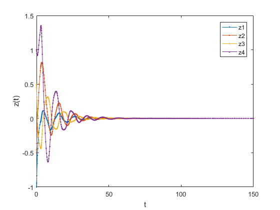
Figure 1: Trajectory of Example 2.

Example 3 [37, 38, 39, 18, 27] Consider the delayed neural network (2.6) with:

$$\begin{array}[]{l}A=\left[\begin{matrix}1&1\\ -1&-1\end{matrix}\right],\ \ B=\left[\begin{matrix}0.88&1\\ 1&1\end{matrix}\right],\ \ C={\rm diag}\{2,2\},\ \ L_{1}=0.4,\ \ L_{2}=0.8.\end{array}$$

This example was studied in [37]. We list the maximal delay bounds of $h(t)$ with different $\mu$ and fixed $k=10^{-6}$ in Table 3. It is obvious that the results obtained by Theorem 3.1 is better than those in [37, 38, 39, 18, 27]. The improvement show the effectiveness and superiority of our method .

Set $z(0)=[-1,1]^{T}$. The trajectory of the delayed system (2.6) with $h(t)=6.3039+0.77sin(t),\ f(z(t))=[0.4tanh(z_{1}(t)),0.8tanh(z_{2}(t))]$ is depicted in Fig. 2.

Table 3: Allowable $h$ for different $\mu$ (Example 3).

$\mu$	0.77	0.80	0.90	NoDVs
[38]	2.3368	1.2281	0.8636	$3.5n^{2}+15.5n$
[39]	2.3368	1.2281	0.8636	$14.5n^{2}+7.5n$
[18]	3.2681	1.6831	1.1493	$2.5n^{2}+15.5n$
Theorem 2 with $N=1$[37]	3.4373	1.8496	1.0904	$22n^{2}+8n$
Theorem 2 with $N=2$[37]	3.5423	1.9149	1.1786	$23.5n^{2}+9.5n$
Theorem 3.1[27]$(k=10^{-6})$	5.8372	3.3805	2.1714	${20.5n^{2}+12.5n}$
Theorem of 3.1$(k=10^{-6})$	7.0739	3.5641	2.2092	${20.5n^{2}+11.5n}$

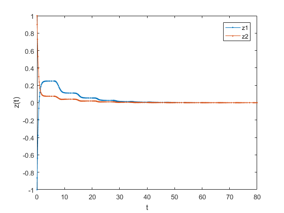
Figure 2: Trajectory of Example 3.

5 Conclusion

Exponential stability for a kind of neural networks having time-varying delay is studied by extend the auxiliary function-based integral inequality with weight functions. This weighted integral inequality is used to analyze a Lyapunov-Krasovskii function to obtain a sharpened criterion for exponential stability. Furthermore, when studying the Lyapunov-Krasovskii function, we find that some decision variables introduced previously can be removed without affecting performance of the proposed criterion. Several examples have been tested to demonstrate the advantages of the new criterion.

References

• [1] W. Zhang, C. Li, T. Huang, M. Xiao, Synchronization of neural networks with stochastic perturbation via aperiodically intermittent control, Neural networks 71 (2015) 105-111.
• [2] R. Yang, B. Wu, Y. Liu, A Halanay-type inequality approach to the stability analysis of discrete-time neural networks with delays, Applied Mathematics and Computation 265 (2015) 696-707.
• [3] H. Shen, Y. Zhu, L. Zhang, J. H. Park, Extended dissipative state estimation for Markov jump neural networks with unreliable links, IEEE Trans. Neural Netw. Learn. Syst. 28 (2017) 346-358.
• [4] H. Yan, H. Zhang, F. Yang, X. Zhan, C. Peng, Event-triggered asynchronous guaranteed cost control for Markov jump discrete-time neural networks with distributed delay and channel fading, IEEE Trans. Neural Netw. Learn. Syst. 29 (2018) 3588-3598.
• [5] L. Zhang, Y. Zhu, W. X. Zheng, Synchronization and state estimation of a class of hierarchical hybrid neural networks with time-varying delays, IEEE Trans. Neural Netw. Learn. Syst. 27 (2016) 459-470.
• [6] C. Marcus, R. Westervelt, Stability of analog neural networks with delay, Phys. Rev. A 39 (1) (1989) 347-359.
• [7] Y. Liu, D. Zhang, J. Lu, J Cao, Global $\mu$-stability criteria for quaternion-valued neural networks with unbounded time-varying delays, Information Sciences 360 (2016) 273-288.
• [8] Y. Liu, P. Xu, J. Lu, J. Liang, Global stability of Clifford-valued recurrent neural networks with time delays, Nonlinear Dynamics 84 (2) (2016) 767-777.
• [9] S. Wen, Z. Zeng, T. Huang, X. Yu, M. Xiao, New criteria of passivity analysis for fuzzy time-delay systems with parameter uncertainties, IEEE Transactions on Fuzzy Systems 23 (6) (2015) 2284-2301.
• [10] W. Li, S. Wang, V. Rehbock, Numerical Solution of Fractional Optimal Control, Journal of Optimization Theory and Applications, 180 (2) (2019) 556-573.
• [11] J. Wang, Z. Yang, T. Huang, M. Xiao, Synchronization criteria in complex dynamical networks with nonsymmetric coupling and multiple time-varying delays, Applicable Analysis 91 (5) (2012) 923-935.
• [12] Y. Zhang, M. Wang, H. Xu, K.L. Teo, Global stabilization of switched control systems with time delay, Nonlinear Analysis: Hybrid Systems 14 (2014) 86-98.
• [13] C. Liu, R. Loxton, K.L. Teo, A computational method for solving time-delay optimal control problems with free terminal time, Systems $\&$ Control Letters 72 (2014) 53-60.
• [14] X. Dai, Y. Huang, M. Xiao, Periodically switched stability induces exponential stability of discrete-time linear switched systems in the sense of Markovian probabilities, Automatica 47 (7) (2011) 1512-1519.
• [15] L.V. Hien, H. Trinh, Exponential stability of time-delay systems via new weighted integral inequalities, Applied Mathematics and Computation 275 (2016) 335-344.
• [16] C. Shi, S. Vong, Finite-time stability for discrete-time systems with time-varying delay and nonlinear perturbations by weighted inequalities, to appear in J. Frankl. Inst.
• [17] S. Vong, C. Shi, Z. Yao, Exponential synchronization of inertial neural networks with mixed delays via weighted integral inequalities, submitted.
• [18] Y. He , G. Liu , D. Rees , New delay-dependent stability criteria for neural networks with time-varying delay, IEEE Trans. Neural Netw. 18 (1) (2007) 310-314 .
• [19] P. G. Park, J. W. Ko, C. Jeong, Reciprocally convex approach to stability of systems with time-varying delays, Automatica 47 (2011) 235-238.
• [20] K. Gu, A further refinement of discretized Lyapunov functional method for the stability of time-delay systems, Int. J. Control 74 (2001) 967-976.
• [21] Z. Wang, L. Liu, Q.H. Shan, H. Zhang, Stability criteria for recurrent neural networks with time-varying delay based on secondary delay partitioning method, IEEE Trans. Neural Netw. Learn. Syst. 26 (2015) 2589-2595.
• [22] Y. He, G. P. Liu, D. Rees, M. Wu, Stability analysis for neural networks with time-varying interval delay, IEEE Trans. Neural Netw. 18 (2017) 1850-1854.
• [23] Z. Li, H. Yan, H. Zhang, X. Zhan, C. Huang, Improved inequality-based functions approach for stability analysis of time delay system. Automatica, DOI: 10.1016/j.automatica.2019.05.033.
• [24] Z. Li, H. Yan, H. Zhang, Y. Peng, J. Park, Y. He, Stability analysis of linear systems with time-varying delay via intermediate polynomial-based functions, Automatica, DOI: 10.1016/j.automatica.2019.108756.
• [25] Z. Li, H. Yan, H. Zhang, J. Sun, H. Lam, Stability and stabilization with additive freedom for delayed Takagi-Sugeno fuzzy systems by intermediary polynomial-based functions. IEEE Transactions on Fuzzy 28 (2010) 692-705.
• [26] Z. Li, H. Yan, H. Zhang, X. Zhan, C. Huang, Stability analysis for delayed neural networks via improved auxiliary polynomial-based functions, IEEE Transactions on Neural Networks and Learning Systems 30 (8) (2019) 2562-2568.
• [27] X.F. Liu, X.G. Liu, M.L. Tang, F.X. Wang, Improved exponential stability criterion for neural networks with time-varying delay, Neurocomputing 234 (2017) 154-163.
• [28] P. Park, W.I. Lee, S.Y. Lee, Auxiliary function-based integral inequalities for quadratic functions and their applications to time-delay systems, J. Frankl. Inst. 352 (2015) 1378-1396.
• [29] L.V. Hien, H. Trinh, Refined Jensen-based inequality approach to stability analysis of time-delay systems, IET Control Theory Appl. 9 (2015) 2188-2194.
• [30] L.V. Hien, H. Trinh, New finite-sum inequalities and their applications to discrete-time delay systems, Automatica 71 (2016) 197-201.
• [31] S.W. Vong, C.Y. Shi, D.D Liu, Improved exponential stability criteria of time-delay systems via weighted integral inequalities, Applied Mathematics Letters 86 (2018) 14-21.
• [32] P. Park, J.W. Ko, C. Jeong, Reciprocally convex approach to stability of systems with time-varying delays, Automatica 47 (2011) 235-238.
• [33] M. Wu, F. Liu, P. Shi, Y. He, R. Yokoyama, Exponential stability analysis for neural networks with time-varying delay, IEEE Trans. Syst. Man Cybern. B Cybern. 38 (2008) 1152-1156.
• [34] C.D. Zheng, H. Zhang, Z. Wang, New delay-dependent global exponential stability criteria for cellular-type neural networks with time-varying delays, IEEE Trans. Circuits Syst. II 56 (2009) 250-254.
• [35] M.D. Ji, Y. He, M. Wu, C.K. Zhang, New exponential stability criterion for neural networks with time-varying delay, in: Proceedings of the 33rd Chinese Control Conference, Nanjing, China, 2014.
• [36] M.D. Ji, Y. He, M. Wu, C.K. Zhang, Further result on exponential stability of neural network with time-varying delay, Appl. Math. Comput. 256 (2015) 175-182.
• [37] W.H. Chen, W.X. Zheng, Improved delay-dependent asymptotic stability criteria for delayed neural networks, IEEE Trans. Neural Netw. 19 (2008) 2154-2161.
• [38] Y. He, Q.G. Wang, M. Wu, LMI-based stability criteria for neural networks with multiple time-varying delays, Physica. D 212 (2005) 126-136.
• [39] C.C. Hua, C.N. Long, X.P. Guan, New results on stability analysis of neural networks with time-varying delays, Phys. Lett. A 352 (2006) 335-340.