Probabilistic Hyperproperties with Nondeterminism

Abstract

We study the problem of formalizing and checking probabilistic hyperproperties for models that allow nondeterminism in actions. We extend the temporal logic HyperPCTL, which has been previously introduced for discrete-time Markov chains, to enable the specification of hyperproperties also for Markov decision processes. We generalize HyperPCTL by allowing explicit and simultaneous quantification over schedulers and probabilistic computation trees and show that it can express important quantitative requirements in security and privacy. We show that HyperPCTL model checking over MDPs is in general undecidable for quantification over probabilistic schedulers with memory, but restricting the domain to memoryless non-probabilistic schedulers turns the model checking problem decidable. Subsequently, we propose an SMT-based encoding for model checking this language and evaluate its performance.

1 Introduction

Hyperproperties [1] extend the conventional notion of trace properties [2] from a set of traces to a set of sets of traces. In other words, a hyperproperty stipulates a system property and not the property of just individual traces. It has been shown that many interesting requirements in computing systems are hyperproperties and cannot be expressed by trace properties. Examples include (1) a wide range of information-flow security policies such as noninterference [3] and observational determinism [4], (2) sensitivity and robustness requirements in cyber-physical systems [5], and consistency conditions such as linearizability in concurrent data structures [6].

Hyperproperties can describe the requirements of probabilistic systems as well. They generally express probabilistic relations between multiple executions of a system. For example, in information-flow security, adding probabilities is motivated by establishing a connection between information theory and information flow across multiple traces. A prominent example is probabilistic schedulers that open up an opportunity for an attacker to set up a probabilistic covert channel. Or, probabilistic causation compares the probability of occurrence of an effect between scenarios where the cause is or is not present.

Figure 1: Example DTMC.

The state of the art on probabilistic hyperproperties has exclusively been studied in the context of discrete-time Markov chains (DTMCs). In [7], we proposed the temporal logic HyperPCTL, which extends PCTL by allowing explicit and simultaneous quantification over computation trees. For example, the DTMC in Fig. 1 satisfies the following HyperPCTL formula:

$$\psi=\forall\hat{s}.\forall\hat{s}^{\prime}.\Big{(}\textit{init}_{\hat{s}}\wedge\textit{init}_{\hat{s}^{\prime}}\Big{)}\Rightarrow\Big{(}\mathbb{P}(\operatorname{\leavevmode\hbox to8.7pt{\vbox to8.7pt{\text{[drawing]}}}}a_{\hat{s}})=\mathbb{P}(\operatorname{\leavevmode\hbox to8.7pt{\vbox to8.7pt{\text{[drawing]}}}}a_{\hat{s}^{\prime}})\Big{)}$$ (1)

which means that the probability of reaching proposition $a$ from any pair of states $\hat{s}$ and $\hat{s}^{\prime}$ labeled by $\mathit{init}$ should be equal. Other works on probabilistic hyperproperties for DTMCs include parameter synthesis [8] and statistical model checking [9, 5].

Figure 2: Example MDP.

An important gap in the spectrum is verification of probabilistic hyperproperties with regard to models that allow nondeterminism, in particular, Markov decision processes (MDP). Nondeterminism plays a crucial role in many probabilistic systems. For instance, nondeterministic queries can be exploited in order to make targeted attacks to databases with private information [10]. To motivate the idea, consider the MDP in Fig. 2, where $h$ is a high secret and $l$ is a low publicly observable variable. To protect the secret, there should be no probabilistic dependencies between observations on the low variable $l$ and the value of $h$. However, an attacker that chooses a scheduler that always takes action $\alpha$ from states $s_{0}$ and $s_{1}$ can learn whether or not $h\leq 0$ by observing the probability of obtaining $l=1$ (or $l=2$). On the other hand, a scheduler that always chooses action $\beta$, does not leak any information about the value of $h$. Thus, a natural question to ask is whether a certain property holds for all or some schedulers.

Figure 3: Example MDP.

With the above motivation, in this paper, we focus on probabilistic hyperproperties in the context of MDPs. Such hyperproperties inherently need to consider different nondeterministic choices in different executions, and naturally call for quantification over schedulers. There are several challenges to achieve this. In general, there are schedulers whose reachability probabilities cannot be achieved by any memoryless non-probabilistic scheduler, and, hence finding a scheduler is not reducible to checking non-probabilistic memoryless schedulers, as it is done in PCTL mode checking for MDPs. Consider for example the MDP in Fig. 3, for which we want to know whether there is a scheduler such that the probability to reach $s_{1}$ from $s_{0}$ equals $0.5$. There are two non-probabilistic memoryless schedulers, one choosing action $\alpha$ and the other, action $\beta$ in $s_{0}$. The first one is the maximal scheduler for which $s_{1}$ is reached with probability $1$, and the second one is the minimal scheduler leading to probability $0$. However, the probability $0.5$ cannot be achieved by any non-probabilistic scheduler. Memoryless probabilistic schedulers can neither achieve probability $0.5$: if a memoryless scheduler would take action $\alpha$ with any positive probability, then the probability to reach $s_{1}$ is always $1$. The only way to achieve the reachability probability $0.5$ (or any value strictly between $0$ and $1$) is by a probabilistic scheduler with memory, e.g., taking $\alpha$ and $\beta$ in $s_{0}$ with probabilities $0.5$ each when this is the first step on a path, and $\beta$ with probability $1$ otherwise.

Our contributions in this paper are as follows. We first extend the temporal logic HyperPCTL [7] to the context of MDPs. To this end, we augment the syntax and semantics of HyperPCTL to quantify over schedulers and relate probabilistic computation trees for different schedulers. For example, the following formula generalizes (1) by requiring that the respective property should hold for all computation trees starting in any states $\hat{s}$ and $\hat{s}^{\prime}$ of the DMTC induced by any scheduler $\hat{\sigma}$:

$$\forall\hat{\sigma}.\forall\hat{s}(\hat{\sigma}).\forall\hat{s}^{\prime}(\hat{\sigma}).\Big{(}\mathit{init}_{\hat{s}}\wedge\mathit{init}_{\hat{s}^{\prime}}\Big{)}\,\Rightarrow\, \Big{(}\mathbb{P}(\operatorname{\leavevmode\hbox to8.7pt{\vbox to8.7pt{\text{[drawing]}}}}a_{\hat{s}})=\mathbb{P}(\operatorname{\leavevmode\hbox to8.7pt{\vbox to8.7pt{\text{[drawing]}}}}a_{\hat{s}^{\prime}})\Big{)}$$

On the negative side, we show that the problem to check HyperPCTL properties for MDPs is in general undecidable. On the positive side, we show that the problem becomes decidable when we restrict the scheduler quantification domain to memoryless non-probabilistic schedulers. We also show that this restricted problem is already NP-complete (respectively, coNP-complete) in the size of the given MDP for HyperPCTL formulas with a single existential (respectively, universal) scheduler quantifier. Subsequently, we propose an SMT-based encoding to solve the restricted model checking problem. We have implemented our method and analyze it experimentally on three case studies: probabilistic scheduling attacks, side-channel timing attacks, and probabilistic conformance (available at https://github.com/oreohere/HyperOnMDP).

It is important to note that the work in [11] (also published in ATVA’20) independently addresses the problem under investigation in this paper. The authors propose the temporal logic PHL. Similar to HyperPCTL, PHL also allows quantification over schedulers, but path quantification of the induced DTMC is achieved by using HyperCTL^∗. Both papers show that the model checking problem is undecidable for the respective logics. The difference, however, is in our approaches to deal with the undecidability result, which leads two complementary and orthogonal techniques. For both logics the problem is decidable for non-probabilistic memoryless schedulers. We provide an SMT-based verification procedure for HyperPCTL for this class of schedulers. The work in [11] presents two methods for proving and for refuting formulas from a fragment of PHL for general memoryful schedulers. The two papers offer disjoint case studies for evaluation.

Organization.

Preliminary concepts are discussed in Section 2. We present the syntax and semantics of HyperPCTL for MDPs and discuss its expressive power in Section 3. Section 4 is dedicated to the applications of HyperPCTL. Sections 5 and 6 present our results on memoryless non-probabilistic schedulers and their evaluation before concluding in Section 7. All proofs are given in the Appendix.

2 Preliminaries

2.1 Discrete-time Markov models

Definition 1

A discrete-time Markov chain (DTMC) is a tuple $\mathcal{D}{=}(S,\mathbf{P},\mathsf{AP},L)$ with the following components:

• $S$ is a nonempty finite set of states;

• $\mathbf{P}:S\times S\rightarrow[0,1]$ is a transition probability function with $\sum_{s^{\prime}\in S}\mathbf{P}(s,s^{\prime})=1$, for all $s\in S$;

• $\mathsf{AP}$ is a finite set of atomic propositions, and

• $L:S\rightarrow 2^{\mathsf{AP}}$ is a labeling function. $~{}\blacksquare$

Fig 1 shows a simple DTMC. An (infinite) path of $\mathcal{D}$ is an infinite sequence $\pi=s_{0}s_{1}s_{2}\ldots\in S^{\omega}$ of states with $\mathbf{P}(s_{i},s_{i+1})>0$, for all $i\geq 0$; we write $\pi[i]$ for $s_{i}$. Let $\mathit{Paths}_{s}^{\mathcal{D}}$ denote the set of all (infinite) paths of $\mathcal{D}$ starting in $s$, and $\mathit{fPaths}_{s}^{\mathcal{D}}$ denote the set of all non-empty finite prefixes of paths from $\mathit{Paths}_{s}^{\mathcal{D}}$, which we call finite paths. For a finite path $\pi=s_{0}\ldots s_{k}\in\mathit{fPaths}_{s_{0}}^{\mathcal{D}}$, $k\geq 0$, we define $|\pi|=k$. We will also use the notations $\mathit{Paths}^{\mathcal{D}}=\cup_{s\in S}\mathit{Paths}_{s}^{\mathcal{D}}$ and $\mathit{fPaths}^{\mathcal{D}}=\cup_{s\in S}\mathit{fPaths}_{s}^{\mathcal{D}}$. A state $t\in S$ is reachable from a state $s\in S$ in $\mathcal{D}$ if there exists a finite path in $\mathit{fPaths}_{s}^{\mathcal{D}}$ with last state $t$; we use $\mathit{fPaths}_{s,T}^{\mathcal{D}}$ to denote the set of all finite paths from $\mathit{fPaths}_{s}^{\mathcal{D}}$ with last state in $T\subseteq S$. A state $s\in S$ is absorbing if $\mathbf{P}(s,s)=1$.

The cylinder set $\textit{Cyl}^{\mathcal{D}}(\pi)$ of a finite path $\pi\in\mathit{fPaths}_{s}^{\mathcal{D}}$ is the set of all infinite paths of $\mathcal{D}$ with prefix $\pi$. The probability space for $\mathcal{D}$ and state $s\in S$ is $(\mathit{Paths}_{s}^{\mathcal{D}},\{\cup_{\pi\in R}\textit{Cyl}^{\mathcal{D}}(\pi)\,|\,R\subseteq\mathit{fPaths}_{s}^{\mathcal{D}}\},\mathrm{Pr}^{\mathcal{D}}_{s})$, where the probability of the cylinderset of $\pi\in\mathit{fPaths}_{s}^{\mathcal{D}}$ is $\mathrm{Pr}^{\mathcal{D}}_{s}(\textit{Cyl}^{\mathcal{D}}(\pi))=\Pi_{i=1}^{|\pi|}\mathbf{P}(\pi[i{-}1],\pi[i])$.

Note that the cylinder sets of two finite paths starting in the same state are either disjoint or one is contained in the other. According to the definition of the probability spaces, the total probability for a set of cylinder sets defined by the finite paths $R\subseteq\mathit{fPaths}_{s}^{\mathcal{D}}$ is $\mathrm{Pr}^{\mathcal{D}}(R)=\sum_{\pi\in R^{\prime}}\mathrm{Pr}^{\mathcal{D}}_{s}(\pi)$ with $R^{\prime}=\{\pi\in R\,|\,\textit{no $\pi^{\prime}\in R\setminus\{\pi\}$ is a prefix of $\pi$}\}$. To improve readability, we sometimes omit the DTMC index $\mathcal{D}$ in the notations when it is clear from the context.

Parallel composition formalizes simultaneous runs in different DTMCs.

Definition 2

The parallel composition of two DTMCs $\mathcal{D}_{i}=(S_{i},\mathbf{P}_{i},\mathsf{AP}_{i},L_{i})$, $i=1,2$, is the DTMC $\mathcal{D}_{1}\times\mathcal{D}_{2}=(S,\mathbf{P},\mathsf{AP},L)$ with the following components:

• $S=S_{1}\times S_{2}$;

• $\mathbf{P}:S\times S\rightarrow[0,1]$ with $\mathbf{P}((s_{1},s_{2}),(s_{1}^{\prime},s_{2}^{\prime}))=\mathbf{P}_{1}(s_{1},s_{1}^{\prime})\cdot\mathbf{P}_{2}(s_{2},s_{2}^{\prime})$, for all states $(s_{1},s_{2}),(s_{1}^{\prime},s_{2}^{\prime})\in S$;

• $\mathsf{AP}=\mathsf{AP}_{1}\cup\mathsf{AP}_{2}$, and

• $L:S\rightarrow 2^{\mathsf{AP}}$ with $L((s_{1},s_{2}))=L_{1}(s_{1})\cup L_{2}(s_{2})$. $~{}\blacksquare$

Markov decision processes extend DTMCs with non-deterministic choices.

Definition 3

A Markov decision process (MDP) is a tuple $\mathcal{M}=(S,\mathit{Act},\mathbf{P},\mathsf{AP},L)$ with the following components:

• $S$ is a nonempty finite set of states;

• $\mathit{Act}$ is a nonempty finite set of actions;

• $\mathbf{P}:S\times\mathit{Act}\times S\rightarrow[0,1]$ is a transition probability function such that for all $s\in S$ the set of enabled actions in $s$ $\mathit{Act}(s)=\{\alpha\in\mathit{Act}\,|\,\sum_{s^{\prime}\in S}\mathbf{P}(s,\alpha,s^{\prime})=1\}$ is not empty and $\sum_{s^{\prime}\in S}\mathbf{P}(s,\alpha,s^{\prime})=0$ for all $\alpha\in\mathit{Act}\setminus\mathit{Act}(s)$;

• $\mathsf{AP}$ is a finite set of atomic propositions, and

• $L:S\rightarrow 2^{\mathsf{AP}}$ is a labeling function. $~{}\blacksquare$

Fig. 2 shows a simple MDP. Schedulers can be used to eliminate the non-determinism in MDPs, inducing DTMCs with well-defined probability spaces.

Definition 4

A scheduler for an MDP $\mathcal{M}=(S,\mathit{Act},\mathbf{P},\mathsf{AP},L)$ is a tuple $\sigma=(Q,\mathit{act},\textit{mode},\mathit{init})$, where

• $Q$ is a countable set of modes;

• $\mathit{act}:Q\times\ S\times\mathit{Act}\rightarrow[0,1]$ is a function for which $\sum_{\alpha\in\mathit{Act}(s)}\mathit{act}(q,s,\alpha)=1$ and $\sum_{\alpha\in\mathit{Act}\setminus\mathit{Act}(s)}\mathit{act}(q,s,\alpha)=0$ for all $s\in S$ and $q\in Q$;

• $\textit{mode}:Q\times S\rightarrow Q$ is a mode transition function, and

• $\mathit{init}:S\rightarrow Q$ is a function selecting a starting mode for each state of $\mathcal{M}$. $~{}\blacksquare$

Let $\Sigma^{\mathcal{M}}$ denote the set of all schedulers for the MDP $\mathcal{M}$. A scheduler is finite-memory if $Q$ is finite, memoryless if $|Q|=1$, and non-probabilistic if $\mathit{act}(q,s,\alpha)\in\{0,1\}$ for all $q\in Q$, $s\in S$ and $\alpha\in\mathit{Act}$.

Definition 5

Assume an MDP $\mathcal{M}=(S,\mathit{Act},\mathbf{P},\mathsf{AP},L)$ and a scheduler $\sigma=(Q,\mathit{act},\textit{mode},\mathit{init})\in\Sigma^{\mathcal{M}}$ for $\mathcal{M}$. The DTMC induced by $\mathcal{M}$ and $\sigma$ is defined as $\mathcal{M}^{\sigma}=(S^{\sigma},\mathbf{P}^{\sigma},\mathsf{AP},L^{\sigma})$ with $S^{\sigma}=Q\times S$,

$$\mathbf{P}^{\sigma}((q,s),(q^{\prime},s^{\prime}))=\left\{\begin{array}[]{l@{\qquad}l}\sum_{\alpha\in\mathit{Act}(s)}\mathit{act}(q,s,\alpha)\cdot\mathbf{P}(s,\alpha,s^{\prime})&\textit{if }q^{\prime}=\textit{mode}(q,s)\\ 0&\textit{otherwise}\end{array}\right.$$

and $L^{\sigma}(q,s)=L(s)$ for all $s,s^{\prime}\in S$ and all $q,q^{\prime}\in Q$. $~{}\blacksquare$

A state $s^{\prime}$ is reachable from $s\in S$ in MDP $\mathcal{M}$ is there exists a scheduler $\sigma$ for $\mathcal{M}$ such that $s^{\prime}$ is reachable from $s$ in $\mathcal{M}^{\sigma}$. A state $s\in S$ is absorbing in $\mathcal{M}$ if $s$ is absorbing in $\mathcal{M}^{\sigma}$ for all schedulers $\sigma$ for $\mathcal{M}$. We sometimes omit the MDP index $\mathcal{M}$ in the notations when it is clear from the context.

3 HyperPCTL for MDPs

In this section we extend HyperPCTL from [7] for DTMCs, to argue also about non-determinism in MDPs.

3.1 HyperPCTL Syntax

HyperPCTL (quantified) state formulas $\varphi^{q}$ are inductively defined as follows:

$$\begin{array}[]{llll}\textit{\small quantified formula}&\varphi^{q}&::=&\forall\hat{\sigma}.\varphi^{q}\ \ |\ \ \exists\hat{\sigma}.\varphi^{q}\ \ |\ \ \forall\hat{s}(\hat{\sigma}).\varphi^{q}\ \ |\ \ \exists\hat{s}(\hat{\sigma}).\varphi^{q}\ \ |\ \ \varphi^{\textit{nq}}\\ \textit{\small non-quantified formula}&\varphi^{\textit{nq}}&::=&\mathtt{true}\ \ |\ \ a_{\hat{s}}\ \ |\ \ \varphi^{\textit{nq}}\wedge\varphi^{\textit{nq}}\ \ |\ \ \neg\varphi^{\textit{nq}}\ \ |\ \ \varphi^{\textit{pr}}<\varphi^{\textit{pr}}\\ \textit{\small probability expression}&\varphi^{\textit{pr}}&::=&\mathbb{P}(\varphi^{\textit{path}})\ \ |\ \ f(\varphi^{\textit{pr}}_{1},\dots,\varphi^{\textit{pr}}_{k})\\ \textit{\small path formula}&\varphi^{\textit{path}}&::=&\operatorname{\leavevmode\hbox to7.41pt{\vbox to7.41pt{\text{[drawing]}}}}\varphi^{\textit{nq}}\ \ |\ \ \varphi^{\textit{nq}}\,\,\mathcal{U}\,\,\varphi^{\textit{nq}}\ \ |\ \ \varphi^{\textit{nq}}\,\,\mathcal{U}\,^{[k_{1},k_{2}]}\,\varphi^{\textit{nq}}\par\end{array}$$

where $\hat{\sigma}$ is a scheduler variable from an infinite set $\hat{\Sigma}$, $\hat{s}$ is a state variable from an infinite set $\hat{S}$, $\varphi^{\textit{nq}}$ is a quantifier-free state formula, $a\in\mathsf{AP}$ is an atomic proposition, $\varphi^{\textit{pr}}$ is a probability expression, $f:[0,1]^{k}\rightarrow\mathbb{R}$ are $k$-ary arithmetic operators (binary addition, unary/binary subtraction, binary multiplication) over probabilities, where constants are viewed as $0$-ary functions, and $\varphi^{\textit{path}}$ is a path formula, such that $k_{1}\leq k_{2}\in\mathbb{N}_{\geq 0}$. The probability operator $\mathbb{P}$ allows the usage of probabilities in arithmetic constraints and relations.

A HyperPCTL construct $\varphi$ (probability expression $\varphi^{\textit{pr}}$, state formula $\varphi^{q}$, $\varphi^{\textit{nq}}$ or path formula $\varphi^{\textit{path}}$) is well-formed if each occurrence of any $a_{\hat{s}}$ with $a\in\mathsf{AP}$ and $\hat{s}\in\hat{S}$ is in the scope of a state quantifier for $\hat{s}(\hat{\sigma})$ for some $\hat{\sigma}\in\hat{\Sigma}$, and any quantifier for $\hat{s}(\hat{\sigma})$ is in the scope of a scheduler quantifier for $\hat{\sigma}$. We restrict ourselves to quantifying first the schedulers then the states, i.e., different state variables can share the same scheduler. One can consider also local schedulers when different players cannot explicitly share the same scheduler, or in other words, each scheduler quantifier belongs to exactly one of the quantified states.

HyperPCTL formulas are well-formed HyperPCTL state formulas, where we additionally allow standard syntactic sugar like $\mathtt{false}=\neg\mathtt{true}$, $\varphi_{1}\vee\varphi_{2}=\neg(\neg\varphi_{1}\wedge\neg\varphi_{2})$, $\operatorname{\leavevmode\hbox to8.7pt{\vbox to8.7pt{\text{[drawing]}}}}\varphi=\mathtt{true}\,\,\mathcal{U}\,\,\varphi$, and $\mathbb{P}(\operatorname{\leavevmode\hbox to6.97pt{\vbox to6.97pt{\text{[drawing]}}}}\varphi)=1-\mathbb{P}(\operatorname{\leavevmode\hbox to8.7pt{\vbox to8.7pt{\text{[drawing]}}}}\neg\varphi)$. For example, the HyperPCTL state formula $\forall\hat{\sigma}.\exists\hat{s}(\hat{\sigma}).\mathbb{P}(\operatorname{\leavevmode\hbox to7.41pt{\vbox to7.41pt{\text{[drawing]}}}}a_{\hat{s}})<0.5$ is a HyperPCTL formula. The HyperPCTL state formula $\mathbb{P}(\operatorname{\leavevmode\hbox to7.41pt{\vbox to7.41pt{\text{[drawing]}}}}a_{\hat{s}}){<}0.5$ is not a HyperPCTL formula, but can be extended to such. The HyperPCTL state formula $\forall\hat{s}(\hat{\sigma}).\exists\hat{\sigma}.\mathbb{P}(\operatorname{\leavevmode\hbox to7.41pt{\vbox to7.41pt{\text{[drawing]}}}}a_{\hat{s}}){<}0.5$ is not a HyperPCTL formula, and it even cannot can be extended to such.

3.2 HyperPCTL Semantics

The semantics of HyperPCTL is based on the $n$-ary self-composition of an MDP.

Definition 6

The n-ary self-composition of an MDP $\mathcal{M}=(S,\mathit{Act},\mathbf{P},\mathsf{AP},L)$ for a sequence $\vec{\sigma}=(\sigma_{1},\ldots,\sigma_{n})\in({\Sigma^{\mathcal{M}}})^{n}$ of schedulers for $\mathcal{M}$ is the DTMC parallel composition $\mathcal{M}^{\vec{\sigma}}=\mathcal{M}_{1}^{\sigma_{1}}\times\ldots\times\mathcal{M}_{n}^{\sigma_{n}}$, where $\mathcal{M}_{i}^{\sigma_{i}}$ is the DTMC induced by $\mathcal{M}_{i}$ and $\sigma_{i}$, and where $\mathcal{M}_{i}=(S,\mathit{Act},\mathbf{P},\mathsf{AP}_{i},L_{i})$ with $\mathsf{AP}_{i}=\{a_{i}\,|\,a\in\mathsf{AP}\}$ and $L_{i}(s)=\{a_{i}\,|\,a\in L(s)\}$, for all $s\in S$. $~{}\blacksquare$

HyperPCTL state formulas are evaluated in the context of an MDP $\mathcal{M}=(S,\mathit{Act},\mathbf{P},\mathsf{AP},L)$, a sequence $\vec{\sigma}=(\sigma_{1},\ldots,\sigma_{n})\in(\Sigma^{\mathcal{M}})^{n}$ of schedulers, and a sequence $\vec{r}=((q_{1},s_{1}),\ldots,(q_{n},s_{n}))$ of $\mathcal{M}^{\vec{\sigma}}$ states; we use $()$ to denote the empty sequence (of any type) and $\circ$ for concatenation. Intuitively, these sequences store instantiations for scheduler and state variables. The satisfaction of a HyperPCTL quantified formula by $\mathcal{M}$ is defined by

$$\mathcal{M}\models\varphi\qquad\textit{iff}\qquad\mathcal{M},(),()\models\varphi\ .$$

The semantics evaluates HyperPCTL formulas by structural recursion. Let in the following $\mathbb{Q},\mathbb{Q}^{\prime},\ldots$ denote quantifiers from $\{\forall,\exists\}$. When instantiating $\mathbb{Q}\hat{\sigma}.\varphi$ by a scheduler $\sigma\in\Sigma^{\mathcal{M}}$, we replace in $\varphi$ each subformula $\mathbb{Q}^{\prime}\hat{s}(\hat{\sigma}).\varphi^{\prime}$, that is not in the scope of a quantifier for $\hat{\sigma}$ by $\mathbb{Q}^{\prime}\hat{s}(\sigma).\varphi^{\prime}$, and denote the result by $\varphi[\hat{\sigma}\leadsto\sigma]$. For instantiating a state quantifier $\mathbb{Q}\hat{s}(\sigma).\varphi$ by a state $s$, we append $\sigma=(Q,\mathit{act},\textit{mode},\mathit{init})$ and $(\mathit{init}(s),s)$ at the end of the respective sequences, and replace each $a_{\hat{s}}$ in the scope of the given quantifier by $a_{s}$, resulting in a formula that we denote by $\varphi[\hat{s}\leadsto s]$. To evaluate probability expressions, we use the $n$-ary self-composition of the MDP.

Formally, the semantics judgment rules are as follows:

$$\begin{array}[]{l@{\quad}c@{\quad}l}\mathcal{M},\vec{\sigma},\vec{r}\models\mathtt{true}\\ \mathcal{M},\vec{\sigma},\vec{r}\models a_{i}&\textit{iff}&a_{i}\in L^{\vec{\sigma}}(\vec{r})\\ \mathcal{M},\vec{\sigma},\vec{r}\models\varphi_{1}\wedge\varphi_{2}&\textit{iff}&\mathcal{M},\vec{\sigma},\vec{r}\models\varphi_{1}\textit{ and }\mathcal{M},\vec{\sigma},\vec{r}\models\varphi_{2}\\ \mathcal{M},\vec{\sigma},\vec{r}\models\neg\varphi&\textit{iff}&\mathcal{M},\vec{\sigma},\vec{r}\not\models\varphi\\ \mathcal{M},\vec{\sigma},\vec{r}\models\forall\hat{\sigma}.\varphi&\textit{iff}&\forall\sigma\in\Sigma^{\mathcal{M}}.\ \mathcal{M},\vec{\sigma},\vec{r}\models\varphi[\hat{\sigma}\leadsto\sigma]\\ \mathcal{M},\vec{\sigma},\vec{r}\models\exists\hat{\sigma}.\varphi&\textit{iff}&\exists\sigma\in\Sigma^{\mathcal{M}}.\ \mathcal{M},\vec{\sigma},\vec{r}\models\varphi[\hat{\sigma}\leadsto\sigma]\\ \mathcal{M},\vec{\sigma},\vec{r}\models\forall\hat{s}(\sigma).\varphi&\textit{iff}&\forall s_{n+1}\in S.\ \mathcal{M},\vec{\sigma}\circ\sigma,\vec{r}\circ(\mathit{init}(s_{n+1}),s_{n+1})\models\varphi[\hat{s}\leadsto s_{n+1}]\\ \mathcal{M},\vec{\sigma},\vec{r}\models\exists\hat{s}(\sigma).\varphi&\textit{iff}&\exists s_{n+1}\in S.\ \mathcal{M},\vec{\sigma}\circ\sigma,\vec{r}\circ(\mathit{init}(s_{n+1}),s_{n+1})\models\varphi[\hat{s}\leadsto s_{n+1}]\\ \mathcal{M},\vec{\sigma},\vec{r}\models\varphi^{\textit{pr}}_{1}<\varphi^{\textit{pr}}_{2}&\textit{iff}&\llbracket\varphi^{\textit{pr}}_{1}\rrbracket_{\mathcal{M},\vec{\sigma},\vec{r}}<\llbracket\varphi^{\textit{pr}}_{2}\rrbracket_{\mathcal{M},\vec{\sigma},\vec{r}}\\ \llbracket\mathbb{P}(\varphi_{\textit{path}})\rrbracket_{\mathcal{M},\vec{\sigma},\vec{r}}&=&\mathrm{Pr}^{\mathcal{M}^{\vec{\sigma}}}\big{(}\{\pi\in\mathit{Paths}_{\vec{r}}^{\mathcal{M}^{\vec{\sigma}}}\mid\mathcal{M},\vec{\sigma},\pi\models\varphi_{\textit{path}}\}\big{)}\\ \llbracket f(\varphi^{\textit{pr}}_{1},\dots\varphi^{\textit{pr}}_{k})\rrbracket_{\mathcal{M},\vec{\sigma},\vec{r}}&=&f\big{(}\llbracket\varphi^{\textit{pr}}_{1}\rrbracket_{\mathcal{M},\vec{\sigma},\vec{r}}\dots,\ \llbracket\varphi^{\textit{pr}}_{k}\rrbracket_{\mathcal{M},\vec{\sigma},\vec{r}}\big{)}\end{array}$$

where $\mathcal{M}$ is an MDP; $n\in\mathbb{N}_{\geq 0}$ is non-negative integer; $\vec{\sigma}\in(\Sigma^{\mathcal{M}})^{n}$; $\vec{r}$ is a state of $\mathcal{M}^{\vec{\sigma}}$; $a\in\mathsf{AP}$ is an atomic proposition and $i\in\{1,\ldots,n\}$; $\varphi,\varphi_{1},\varphi_{2}$ are HyperPCTL state formulas; $\sigma=(Q,\mathit{act},\textit{mode},\mathit{init})\in\Sigma^{\mathcal{M}}$ is a scheduler for $\mathcal{M}$; $\varphi^{\textit{pr}}_{1}\cdots\varphi^{\textit{pr}}_{k}$ are probability expressions, and $\varphi_{\textit{path}}$ is a HyperPCTL path formula whose satisfaction relation is as follows:

$$\begin{array}[]{l@{\ }c@{\ \ }l}\mathcal{M},\vec{\sigma},\pi\models\operatorname{\leavevmode\hbox to6.66pt{\vbox to6.66pt{\text{[drawing]}}}}\varphi&\textit{iff}&\mathcal{M},\vec{\sigma},\vec{r}_{1}\models\varphi\\ \mathcal{M},\vec{\sigma},\pi\models\varphi_{1}\,\mathcal{U}\,\varphi_{2}&\textit{iff}&\exists j\geq 0.\Big{(}\mathcal{M},\vec{\sigma},\vec{r}_{j}\models\varphi_{2}\wedge\forall i\in[0,j).\ \mathcal{M},\vec{\sigma},\vec{r}_{i}\models\varphi_{1}\Big{)}\\ \mathcal{M},\vec{\sigma},\pi\models\varphi_{1}\,\mathcal{U}\,^{[k_{1},k_{2}]}\,\varphi_{2}&\textit{iff}&\exists j\in[k_{1},k_{2}].\Big{(}\mathcal{M},\vec{\sigma},\vec{r}_{j}\models\varphi_{2}\wedge\forall i\in[0,j).\mathcal{M},\vec{\sigma},\vec{r}_{i}\models\varphi_{1}\Big{)}\end{array}$$

where $\pi=\vec{r}_{0}\vec{r}_{1}\cdots$ with $\vec{r}_{i}=((q_{i,1},s_{i,1}),\ldots,(q_{i,n},s_{i,n}))$ is a path of $\mathcal{M}^{\vec{\sigma}}$; formulas $\varphi$, $\varphi_{1}$, and $\varphi_{2}$ are HyperPCTL state formulas, and $k_{1}\leq k_{2}\in\mathbb{N}_{\geq 0}$.

3.3 The Expressiveness Power of HyperPCTL

For MDPs with $|\mathit{Act}(s)|=1$ for each of its states $s$, the HyperPCTL semantics reduces to the one proposed in [7] for DTMCs.

For MDPs with non-determinism, the standard PCTL semantics defines that in order to satisfy a PCTL formula $\mathbb{P}_{\sim c}(\psi)$ in a given MDP state $s$, all schedulers should induce a DTMC that satisfies $\mathbb{P}_{\sim c}(\psi)$ in $s$. Though it should hold for all schedulers, it is known that there exist minimal and maximal schedulers that are non-probabilistic and memoryless, therefore it is sufficient to restrict the reasoning to such schedulers. Since for MDPs with finite state and action spaces, the number of such schedulers is finite, PCTL model checking for MDPs is decidable. Given this analogy, one would expect that HyperPCTL model checking should be decidable, but it is not.

Theorem 3.1

HyperPCTL model checking for MDPs is in general undecidable.

What is the source of increased expressiveness that makes HyperPCTL undecidable? State quantification cannot be the source, as the state space is finite and thus there are finitely many possible state quantifier instantiations.

Assume an MDP $\mathcal{M}=(S,\mathit{Act},\mathbf{P},\mathsf{AP},L)$ with a state $s\in S$ that is uniquely labelled by the proposition $\textit{init}\in L(s)$, and let $a,b\in\mathsf{AP}$. In PCTL, each probability bound needs to be satisfied under all schedulers. For example:

$$\mathcal{M},s\models_{\textsf{\small PCTL}}\mathbb{P}_{<0.5}(a\,\mathcal{U}\,b)\textit{\ iff \ }\mathcal{M}\models_{\textsf{\small HyperPCTL}}\forall\hat{\sigma}.\forall\hat{s}(\hat{\sigma}).(\textit{init}_{\hat{s}}\rightarrow\mathbb{P}(a\,\mathcal{U}\,b)<0.5)$$

Alternatively, we can state:

$$\mathcal{M},s\models_{\textsf{\small PCTL}}\mathbb{P}_{{<}0.5}(a\,\mathcal{U}\,b)\ \ \textit{iff}\ \ \forall\sigma{\in}\Sigma^{\mathcal{M}}\!\!.\mathcal{M},(\sigma),((\mathit{init}_{\sigma}(s),s))\models_{\textsf{\small HyperPCTL}}\mathbb{P}(a\mathcal{U}b){<}0.5$$

where $\mathit{init}_{\sigma}(s)$ is the starting mode of scheduler $\sigma$ in state $s$. Generally, the HyperPCTL fragment which starts with a single universal scheduler quantifier and contains a single bound on a single probability operator is still decidable. However, when a PCTL formula has several probability bounds, its satisfaction requires each bound to be satisfied by all schedulers independently. For example,

$$\mathcal{M},s\models_{\textsf{\small PCTL}}\Big{(}\mathbb{P}_{<0.5}(a\,\mathcal{U}\,b)\;\vee\;\mathbb{P}_{>0.5}(a\,\mathcal{U}\,b)\Big{)}\quad\textit{iff}$$

$$\forall\sigma\in\Sigma^{\mathcal{M}}.\quad\mathcal{M},(\sigma),((\mathit{init}_{\sigma}(s),s))\models_{\textsf{\small HyperPCTL}}\mathbb{P}(a\,\mathcal{U}\,b)<0.5\quad\textit{or}$$

$$\phantom{\forall\sigma\in\Sigma^{\mathcal{M}}.}\quad\mathcal{M},(\sigma),((\mathit{init}_{\sigma}(s),s))\models_{\textsf{\small HyperPCTL}}\mathbb{P}(a\,\mathcal{U}\,b)>0.5$$

This is not equivalent to the HyperPCTL formula

$$\mathcal{M}\models_{\textsf{\small HyperPCTL}}\forall\hat{\sigma}.\forall\hat{s}(\hat{\sigma}).(\textit{init}_{\hat{s}}\rightarrow(\mathbb{P}(a_{\hat{s}}\,\mathcal{U}\,b_{\hat{s}})<0.5\vee\mathbb{P}(a_{\hat{s}}\,\mathcal{U}\,b_{\hat{s}})>0.5))$$

which states that the probability is either less than or larger than $0.5$ under all schedulers, which is true if there exists no scheduler under which the probability is $0.5$ (see also [12]). Thus, even for a fragment restricted to universal scheduler quantification, combinations of probability bounds allows HyperPCTL to express existential scheduler synthesis problems.

Finally, consider a scheduler quantifier followed by state quantifiers, whose scope may contain probability expressions. This means we start several “experiments” in parallel, each one represented by a state quantifier. However, we may use in all experiments the same scheduler. Informally, this allows us to express the existence or absence of schedulers with certain probabilistic hyperproperties for the induced DTMCs. It would however also make sense to flip this quantifier order, such that state quantifiers are followed by scheduler quantifiers. This would mean, that we can use different schedulers in the different concurrently running experiments. This would be meaningful e.g. when users can provide input to the system, i.e. when the scheduler choice lies by the “observers” of the individual experiments, and they can adapt their schedulers to observations made in the other concurrently running experiments.

4 Applications of HyperPCTL on MDPs

⬇

1void mexp(){

2 c = 0; d = 1; i = k;

3 while (i >= 0){

4 i = i-1; c = c*2;

5 d = (d*d) % n;

6 if (b(i) = 1)

7 c = c+1;

8 d = (d*a) % n;

9 }

10}

11/************/

12t = new Thread(mexp());

13j = 0; m = 2 * k;

14while (j < m & !t.stop) j++;

15/************/

Figure 4: Modular exponentiation.

Side-channel timing leaks

open a channel to an attacker to infer the value of a secret by observing the execution time of a function. For example, the heart of the RSA public-key encryption algorithm is the modular exponentiation algorithm that computes $(a^{b}\mod n)$, where $a$ is an integer representing the plaintext and $b$ is the integer encryption key. A careless implementation can leak $b$ through a probabilistic scheduling channel (see Fig. 4). This program is not secure since the two branches of the if have different timing behaviors. Under a fair execution scheduler for parallel threads, an attacker thread can infer the value of $b$ by running in parallel to a modular exponentiation thread and iteratively incrementing a counter variable until the other thread terminates (lines 12-14). To model this program by an MDP, we can use two nondeterministic actions for the two branches of the if statement, such that the choice of different schedulers corresponds to the choice of different bit configurations b(i) for the key b. This algorithm should satisfy the following property: the probability of observing a concrete value in the counter j should be independent of the bit configuration of the secret key b:

$$\forall\hat{\sigma}_{1}.\forall\hat{\sigma}_{2}.\forall\hat{s}(\hat{\sigma}_{1}).\forall\hat{s}^{\prime}(\hat{\sigma}_{2}).\Big{(}init_{\hat{s}}\,\wedge\,init_{\hat{s}^{\prime}}\Big{)}\;\Rightarrow\;\bigwedge_{l=0}^{m}\Big{(}\mathbb{P}(\operatorname{\leavevmode\hbox to8.7pt{\vbox to8.7pt{\text{[drawing]}}}}(j=l)_{\hat{s}})=\mathbb{P}(\operatorname{\leavevmode\hbox to8.7pt{\vbox to8.7pt{\text{[drawing]}}}}(j=l)_{\hat{s}^{\prime}})\Big{)}$$

⬇

1int str_cmp(char * r){

2 char * s = ’Bg\$4\0’;

3 i = 0;

4 while (s[i] != ’\0’){

5 i++;

6 if (s[i]!=r[i]) return 0;

7 }

8 return 1;

9}

Figure 5: String comparison.

Another example of timing attacks that can be implemented through a probabilistic scheduling side channel is password verification which is typically implemented by comparing an input string with another confidential string (see Fig 5). Also here, an attacker thread can measure the time necessary to break the loop, and use this information to infer the prefix of the input string matching the secret string.

Scheduler-specific observational determinism policy

(SSODP) [13] is a confidentiality policy in multi-threaded programs that defends against an attacker that chooses an appropriate scheduler to control the set of possible traces. In particular, given any scheduler and two initial states that are indistinguishable with respect to a secret input (i.e., low-equivalent), any two executions from these two states should terminate in low-equivalent states with equal probability. Formally, given a proposition $h$ representing a secret:

$$\forall\hat{\sigma}.\forall\hat{s}(\hat{\sigma}).\forall\hat{s}^{\prime}(\hat{\sigma}).\big{(}h_{\hat{s}}\oplus h_{\hat{s}^{\prime}}\big{)}\,\Rightarrow\,\bigwedge_{l\in L}\big{(} \mathbb{P}(\operatorname{\leavevmode\hbox to8.7pt{\vbox to8.7pt{\text{[drawing]}}}}l_{\hat{s}})=\mathbb{P}(\operatorname{\leavevmode\hbox to8.7pt{\vbox to8.7pt{\text{[drawing]}}}}l_{\hat{s}^{\prime}})\big{)}$$

where $l\in L$ are atomic propositions that classify low-equivalent states and $\oplus$ is the exclusive-or operator. A stronger variation of this policy is that the executions are stepwise low-equivalent:

$$\forall\hat{\sigma}.\forall\hat{s}(\hat{\sigma}).\forall\hat{s}^{\prime}(\hat{\sigma}).\big{(}h_{\hat{s}}\oplus h_{\hat{s}^{\prime}}\big{)}\,\Rightarrow\,\mathbb{P}\operatorname{\leavevmode\hbox to6.97pt{\vbox to6.97pt{\text{[drawing]}}}}\big{(}\bigwedge_{l\in L}\big{(}(\mathbb{P}\operatorname{\leavevmode\hbox to7.41pt{\vbox to7.41pt{\text{[drawing]}}}}l_{\hat{s}})=(\mathbb{P}\operatorname{\leavevmode\hbox to7.41pt{\vbox to7.41pt{\text{[drawing]}}}}l_{\hat{s}^{\prime}})\big{)}\big{)}=1.$$

Probabilistic conformance

describes how well a model and an implementation conform with each other with respect to a specification. As an example, consider a 6-sided die. The probability to obtain one possible side of the die is $1/6$. We would like to synthesize a protocol that simulates the 6-sided die behavior only by repeatedly tossing a fair coin. We know that such an implementation exists [14], but our aim is to find such a solution automatically by modeling the die as a DTMC and by using an MDP to model all the possible coin-implementations with a given maximum number of states, including 6 absorbing final states to model the outcomes. In the MDP, we associate to each state a set of possible nondeterministic actions, each of them choosing two states as successors with equal probability $1/2$. Then, each scheduler corresponds to a particular implementation. Our goal is to check whether there exists a scheduler that induces a DTMC over the MDP, such that repeatedly tossing a coin simulates die-rolling with equal probabilities for the different outcomes:

$$\exists\hat{\sigma}.\forall\hat{s}(\hat{\sigma}).\exists\hat{s}^{\prime}(\hat{\sigma}).\Big{(}init_{\hat{s}}\,\wedge\,init_{\hat{s}^{\prime}}\Big{)}\;\Rightarrow\;\bigwedge_{l=1}^{6}\Big{(}\mathbb{P}(\operatorname{\leavevmode\hbox to8.7pt{\vbox to8.7pt{\text{[drawing]}}}}(die=l)_{\hat{s}})=\mathbb{P}(\operatorname{\leavevmode\hbox to8.7pt{\vbox to8.7pt{\text{[drawing]}}}}(die=l)_{\hat{s}^{\prime}})\Big{)}$$

5 HyperPCTL Model Checking for Non-probabilistic Memoryless Schedulers

Due to the undecidability of model checking HyperPCTL formulas for MDPs, we noe restrict ourselves the semantics, where scheduler quantification ranges over non-probabilistic memoryless schedulers only. It is easy to see that this restriction makes the model checking problem decidable, as there are only finitely many such schedulers that can be enumerated. Regarding complexity, we have the following property.

Theorem 5.1

The problem to decide for MDPs the truth of HyperPCTL formulas with a single existential (respectively, universal) scheduler quantifier over non-probabilistic memoryless schedulers is NP-complete (respectively, coNP-complete) in the state set size of the given MDP.

Next we propose an SMT-based technique for solving the model checking problem for non-probabilistic memoryless scheduler domains, and for the simplified case of having a single scheduler quantifier; the general case for an arbitrary number of scheduler quantifiers is similar, but a bit more involved, so the simplified setting might be more suitable for understanding the basic ideas.

Input : $\mathcal{M}=(S,\mathit{Act},\mathbf{P},\mathsf{AP},L)$: MDP;

$Q\hat{\sigma}.Q_{1}\hat{s}_{1}(\hat{\sigma}).\ldots Q_{n}\hat{s}_{n}(\hat{\sigma}).\varphi^{\textit{nq}}$: HyperPCTL formula.

Output : Whether $\mathcal{M}$ satisfies the input formula.

1 Function Main$(\mathcal{M}$,  $Q\hat{\sigma}.\ Q_{1}\hat{s}_{1}(\hat{\sigma}).\ldots Q_{n}\hat{s}_{n}(\hat{\sigma}).\ \varphi^{\textit{nq}})$

       $E$ := $\bigwedge_{s\in S}(\bigvee_{\alpha\in\mathit{Act}(s)}\sigma_{s}=\alpha)$ // scheduler choice

2       if $Q$ is existential then

3             $E$ := $E\wedge$ Semantics$(\mathcal{M}$, $\varphi^{\textit{nq}}$, $n)$;

4             $E$ := $E\wedge$ Truth$(\mathcal{M}$, $\exists\hat{\sigma}.\ Q_{1}\hat{s}_{1}(\hat{\sigma}).\ldots Q_{n}\hat{s}_{n}(\hat{\sigma}).\ \varphi^{\textit{nq}})$;

5             if check$(E)$ = SAT then return TRUE;

6            else return FALSE;

7            

8      else if $Q$ is universal then

             // $\overline{Q}_{i}$ is $\forall$ if $Q_{i}=\exists$ and $\exists$ else

9             $E$ := $E\wedge$ Semantics$(\mathcal{M},\neg\varphi^{\textit{nq}},n)$;

10             $E$ := $E\wedge$ Truth$(\mathcal{M}$, $\exists\hat{\sigma}.\overline{Q}_{1}\hat{s}_{1}(\hat{\sigma}).\ldots\overline{Q}_{n}\hat{s}_{n}(\hat{\sigma}).\neg\varphi^{\textit{nq}})$;

11             if check$(E)$ = SAT then return FALSE;

12            else return TRUE;

13            

14      

Algorithm 1 Main SMT encoding algorithm

The main method listed in Algorithm 1 constructs a formula $E$ that is satisfiable if and only if the input MDP $\mathcal{M}$ satisfies the input HyperPCTL formula with a single scheduler quantifier over the non-probabilistic memoryless scheduler domain. Let us first deal with the case that the scheduler quantifier is existential. In line 1 we encode possible instantiations $\sigma$ for the scheduler variable $\hat{\sigma}$, for which we use a variable $\sigma_{s}$ for each MDP state $s\in S$ to encode which action is chosen in that state. In line 1 we encode the meaning of the quantifier-free inner part $\varphi^{\textit{nq}}$ of the input formula, whereas line 1 encodes the meaning of the state quantifiers, i.e. for which sets of composed states $\varphi^{\textit{nq}}$ needs to hold in order to satisfy the input formula. In lines 1–1 we check the satisfiability of the encoding and return the corresponding answer. Formulas with a universal scheduler quantifier $\forall\hat{\sigma}.\varphi$ are semantically equivalent to $\neg\exists\hat{\sigma}.\neg\varphi$. We make use of this fact in lines 1–1 to check first the satisfaction of an encoding for $\exists\hat{\sigma}.\neg\varphi$ and return the inverted answer.

Input : $\mathcal{M}=(S,\mathit{Act},\mathbf{P},\mathsf{AP},L)$: MDP;

$\varphi$: quantifier-free HyperPCTL formula or expression;

$n$: number of state variables in $\varphi$.

Output : SMT encoding of the meaning of $\varphi$ in the $n$-ary self-composition of $\mathcal{M}$.

1 Function Semantics$(\mathcal{M}$, $\varphi$, $n)$

2       if $\varphi$ is $\mathtt{true}$ then  $E$ := $\bigwedge_{\vec{s}\in S^{n}}\textit{holds}_{\vec{s},\varphi}$;

3       else if $\varphi$ is $a_{\hat{s}_{i}}$ then

4             $E$ := $(\bigwedge_{\vec{s}\in S^{n},\ a\in L(s_{i})}(\textit{holds}_{\vec{s},\varphi}))\wedge(\bigwedge_{\vec{s}\in S^{n},\ a\notin L(s_{i})}(\neg\textit{holds}_{\vec{s},\varphi}))$;

5      else if $\varphi$ is $\varphi_{1}\wedge\varphi_{2}$ then

6             $E$ := Semantics$(\mathcal{M},\varphi_{1},n)\wedge$ Semantics$(\mathcal{M},\varphi_{2},n)\wedge$

7              $\bigwedge_{\vec{s}\in S^{n}}((\textit{holds}_{\vec{s},\varphi}{\wedge}\textit{holds}_{\vec{s},\varphi_{1}}{\wedge}\textit{holds}_{\vec{s},\varphi_{2}})\vee(\neg\textit{holds}_{\vec{s},\varphi}{\wedge}(\neg\textit{holds}_{\vec{s},\varphi_{1}}{\vee}\neg\textit{holds}_{\vec{s},\varphi_{2}})))$;

8            

9      else if $\varphi$ is $\neg\varphi^{\prime}$ then

10             $E$ := Semantics$(\mathcal{M},\varphi^{\prime},n)\wedge\bigwedge_{\vec{s}\in S^{n}}(\textit{holds}_{\vec{s},\varphi}\oplus\textit{holds}_{\vec{s},\varphi^{\prime}})$;

11            

12      else if $\varphi$ is $\varphi_{1}<\varphi_{2}$ then

13             $E$ := Semantics$(\mathcal{M}$, $\varphi_{1},n)\wedge$ Semantics$(\mathcal{M}$, $\varphi_{2},n)\wedge$

14              $\bigwedge_{\vec{s}\in S^{n}}((\textit{holds}_{\vec{s},\varphi}\wedge\textit{prob}_{\vec{s},\varphi_{1}}<\textit{prob}_{\vec{s},\varphi_{2}})\vee(\neg\textit{holds}_{\vec{s},\varphi}\wedge\textit{prob}_{\vec{s},\varphi_{1}}\geq\textit{prob}_{\vec{s},\varphi_{2}}))$;

15            

16      else if $\varphi$ is $\mathbb{P}(\operatorname{\leavevmode\hbox to7.41pt{\vbox to7.41pt{\text{[drawing]}}}}\varphi^{\prime})$ then

17             $E$ := Semantics$(\mathcal{M}$, $\varphi^{\prime},n)\wedge$

18              $\bigwedge_{\vec{s}\in S^{n}}\big{(}(\textit{holdsToInt}_{\vec{s},\varphi^{\prime}}=1\wedge\textit{holds}_{\vec{s},\varphi^{\prime}})\vee(\textit{holdsToInt}_{\vec{s},\varphi^{\prime}}=0\wedge\neg\textit{holds}_{\vec{s},\varphi^{\prime}})\big{)}$;

19             foreach $\vec{s}=(s_{1},\ldots,s_{n})\in S^{n}$ do

20                   foreach $\vec{\alpha}=(\alpha_{1},\ldots,\alpha_{n})\in\mathit{Act}(s_{1})\times\ldots\times\mathit{Act}(s_{n})$ do

21                         $E$ := $E\wedge\big{(}\big{[}\bigwedge_{i=1}^{n}\sigma_{s_{i}}=\alpha_{i}\big{]}\rightarrow\big{[}\textit{prob}_{\vec{s},\varphi}=$

22                         $\sum_{\vec{s}^{\prime}\in\mathit{supp}(\alpha_{1})\times\ldots\times\mathit{supp}(\alpha_{n})}((\Pi_{i=1}^{n}\mathbf{P}(s_{i},\alpha_{i},s_{i}^{\prime}))\cdot\textit{holdsToInt}_{\vec{s}^{\prime},\varphi^{\prime}})\big{]}\big{)}$;

23                  

24            

25      else if $\varphi$ is $\mathbb{P}(\varphi_{1}\,\mathcal{U}\,\varphi_{2})$ then  $E$ := SemanticsUnboundedUntil($\mathcal{M}$, $\varphi$, $n$);

26       else if $\varphi$ is $\mathbb{P}(\varphi_{1}\,\mathcal{U}\,^{[k_{1},k_{2}]}\varphi_{2})$ then  $E$ := SemanticsBoundedUntil($\mathcal{M}$, $\varphi$, $n$);

27       else if $\varphi$ is $c$ then  $E$ := $\bigwedge_{\vec{s}\in S^{n}}(\textit{prob}_{\vec{s},\varphi}=c)$;

28       else if $\varphi$ is $\varphi_{1}\textit{ op }\varphi_{2}$  /* $\textit{op}\in\{+,-,*\}$ */   then

29             $E$ := Semantics$(\mathcal{M}$, $\varphi_{1},n)\wedge$ Semantics$(\mathcal{M}$, $\varphi_{2},n)\wedge$ $\bigwedge_{\vec{s}\in S^{n}}(\textit{prob}_{\vec{s},\varphi}=(\textit{prob}_{\vec{s},\varphi_{1}}\textit{ op }\textit{prob}_{\vec{s},\varphi_{2}}))$;

30      return $E$;

Algorithm 2 SMT encoding for the meaning of the input formula

The Semantics method, shown in Algorithm 2, applies structural recursion to encode the meaning of its quantifier-free input formula. As variables, the encoding uses (1) propositions $\textit{holds}_{\vec{s},\varphi^{\textit{nq}}}\in\{\mathtt{true},\mathtt{false}\}$ to encode the truth of each Boolean sub-formula $\varphi^{\textit{nq}}$ of the input formula in each state $\vec{s}\in S^{n}$ of the $n$-ary self-composition of $\mathcal{M}$, (2) numeric variables $\textit{prob}_{\vec{s},\varphi^{\textit{pr}}}\in[0,1]\subseteq\mathbb{R}$ to encode the value of each probability expression $\varphi^{\textit{pr}}$ in the input formula in the context of each composed state $\vec{s}\in S^{n}$, (3) variables $\textit{holdsToInt}_{\vec{s},\varphi^{\textit{pr}}}\in\{0,1\}$ to encode truth values in a pseudo-Boolean form, i.e. we set $\textit{holdsToInt}_{\vec{s},\varphi^{\textit{pr}}}=1$ for $\textit{holds}_{\vec{s},\varphi^{\textit{nq}}}=\mathtt{true}$ and $\textit{prob}_{\vec{s},\varphi^{\textit{pr}}}=0$ else and (4) variables $d_{\vec{s},\varphi}$ to encode the existence of a loop-free path from state $\vec{s}$ to a state satisfying $\varphi$.

There are two base cases: the Boolean constant true holds in all states (line 2), whereas atomic propositions hold in exactly those states that are labelled by them (line 2). For conjunction (line 2) we recursively encode the truth values of the operands and state that the conjunction is true iff both operands are true. For negation (line 2) we again encode the meaning of the operand recursively and flip its truth value. For the comparison of two probability expressions (line 2), we recursively encode the probability values of the operands and state the respective relation between them for the satisfaction of the comparison.

The remaining cases encode the semantics of probability expressions. The cases for constants (line 2) and arithmetic operations (line 2) are straightforward. For the probability $\mathbb{P}(\operatorname{\leavevmode\hbox to7.41pt{\vbox to7.41pt{\text{[drawing]}}}}\varphi^{\prime})$ (line 2), we encode the Boolean value of $\varphi^{\prime}$ in the variables $\textit{holds}_{\vec{s},\varphi^{\prime}}$ (line 2), turn them into pseudo-Boolean values $\textit{holdsToInt}_{\vec{s},\varphi^{\prime}}$ ($1$ for true and $0$ for false, line 2), and state that for each composed state, the probability value of $\mathbb{P}(\operatorname{\leavevmode\hbox to7.41pt{\vbox to7.41pt{\text{[drawing]}}}}\varphi^{\prime})$ is the sum of the probabilities to get to a successor state where the operand $\varphi^{\prime}$ holds; since the successors and their probabilities are scheduler-dependent, we need to iterate over all scheduler choices and use $\mathit{supp}(\alpha_{i})$ to denote the support $\{s\in S\,\ \,\alpha_{i}(s)>0\}$ of the distribution $\alpha_{i}$ (line 2). The encodings for the probabilities of unbounded until formulas (line 2) and bounded until formulas (line 2) are listed in Algorithm 3 and 4, respectively.

Input : $\mathcal{M}=(S,\mathit{Act},\mathbf{P},\mathsf{AP},L)$: MDP; $\varphi$: HyperPCTL unbounded until formula of the form $\mathbb{P}(\varphi_{1}\,\mathcal{U}\,\varphi_{2})$; $n$: number of state variables in $\varphi$.

Output : SMT encoding of $\varphi$’s meaning in the $n$-ary self-composition of $\mathcal{M}$.

1 Function SemanticsUnboundedUntil$(\mathcal{M}$, $\varphi=\mathbb{P}(\varphi_{1}\,\mathcal{U}\,\varphi_{2})$, $n)$

2       $E$ := Semantics$(\mathcal{M}$, $\varphi_{1},n)\wedge$ Semantics$(\mathcal{M}$, $\varphi_{2},n)$;

3       foreach $\vec{s}=(s_{1},\ldots,s_{n})\in S^{n}$ do

4             $E$ := $E\wedge(\textit{holds}_{\vec{s},\varphi_{2}}\rightarrow\textit{prob}_{\vec{s},\varphi}{=}1)\wedge((\neg\textit{holds}_{\vec{s},\varphi_{1}}\wedge\neg\textit{holds}_{\vec{s},\varphi_{2}})\rightarrow\textit{prob}_{\vec{s},\varphi}{=}0)$;

5             foreach $\vec{\alpha}=(\alpha_{1},\ldots,\alpha_{n})\in\mathit{Act}(s_{1})\times\ldots\times\mathit{Act}(s_{n})$ do

6                   $E$ := $E\wedge\Big{(}\big{[}\textit{holds}_{\vec{s},\varphi_{1}}\wedge\neg\textit{holds}_{\vec{s},\varphi_{2}}\wedge\bigwedge_{i=1}^{n}\sigma_{s_{i}}=\alpha_{i}\big{]}\rightarrow$

7                   $\big{[}\textit{prob}_{\vec{s},\varphi}=\sum_{\vec{s}^{\prime}\in\mathit{supp}(\alpha_{1})\times\ldots\times\mathit{supp}(\alpha_{n})}((\Pi_{i=1}^{n}\mathbf{P}(s_{i},\alpha_{i},s_{i}^{\prime}))\cdot\textit{prob}_{\vec{s}^{\prime},\varphi})\wedge$

8                   $(\textit{prob}_{\vec{s},\varphi}{>}0\rightarrow(\bigvee_{\vec{s}^{\prime}\in\mathit{supp}(\alpha_{1})\times\ldots\times\mathit{supp}(\alpha_{n})}(\textit{holds}_{\vec{s}^{\prime},\varphi_{2}}{\vee}d_{\vec{s},\varphi_{2}}{>}d_{\vec{s}^{\prime},\varphi_{2}})))\big{]}\Big{)}$;

9                  

10            

11      return $E$;

Algorithm 3 SMT encoding for the meaning of unbounded until formulas

For the probabilities $\mathbb{P}(\varphi_{1}\,\mathcal{U}\,\varphi_{2})$ to satisfy an unbounded until formula, the method SemanticsUnboundedUntil shown in Algorithm 3 first encodes the meaning of the until operands (line 3). For each composed state $\vec{s}\in S^{n}$, the probability of satisfying the until formula in $\vec{s}$ is encoded in the variable $\textit{prob}_{\vec{s},\mathbb{P}(\varphi_{1}\,\mathcal{U}\,\varphi_{2})}$. If the second until-operand $\varphi_{2}$ holds in $\vec{s}$ then this probability is $1$ and if none of the operands are true in $\vec{s}$ then it is $0$ (line 3). Otherwise, depending on the scheduler $\sigma$ of $\mathcal{M}$ (line 3), the value of $\textit{prob}_{\vec{s},\mathbb{P}(\varphi_{1}\,\mathcal{U}\,\varphi_{2})}$ is a sum, adding up for each successor state $\vec{s}^{\prime}$ of $\vec{s}$ the probability to get from $\vec{s}$ to $\vec{s}^{\prime}$ in one step times the probability to satisfy the until-formula on paths starting in $\vec{s}^{\prime}$ (line 3). However, these encodings work only when at least one state satisfying $\varphi_{2}$ is reachable from $\vec{s}$ with a positive probability: for any bottom SCC whose states all violate $\varphi_{2}$, the probability $\mathbb{P}(\varphi_{1}\,\mathcal{U}\,\varphi_{2})$ is obviously $0$, however, assigning any fixed value from $[0,1]$ to all states of this bottom SCC would yield a fixed-point for the underlying equation system. To assure correctness, in line 3 we enforce smallest fixed-points by requiring that if $\textit{prob}_{\vec{s},\mathbb{P}(\varphi_{1}\,\mathcal{U}\,\varphi_{2})}$ is positive then there exists a loop-free path from $\vec{s}$ to any state satisfying $\varphi_{2}$. In the encoding of this property we use fresh variables $d_{\vec{s},\varphi_{2}}$ and require a path over states with strong monotonically decreasing $d_{\vec{s},\varphi_{2}}$-values to a $\varphi_{2}$-state (where the decreasing property serves to exclude loops). The domain of the distance-variables $d_{\vec{s},\varphi_{2}}$ can be e.g. integers, rationals or reals; the only restriction is that is should contain at least $|S|^{n}$ ordered values. Especially, it does not need to be lower bounded (note that each solution assigns to each $d_{\vec{s},\varphi_{2}}$ a fixed value, leading a finite number of distance values).

Input : $\mathcal{M}=(S,\mathit{Act},\mathbf{P},\mathsf{AP},L)$: MDP; $\varphi$: HyperPCTL bounded until formula of the form $\mathbb{P}(\varphi_{1}\,\mathcal{U}\,^{[k_{1},k_{2}]}\varphi_{2})$; $n$: number of state variables in $\varphi$.

Output : SMT encoding of $\varphi$’s meaning in the $n$-ary self-composition of $\mathcal{M}$.

1 Function SemanticsBoundedUntil$(\mathcal{M}$, $\varphi=\mathbb{P}(\varphi_{1}\,\mathcal{U}\,^{[k_{1},k_{2}]}\varphi_{2})$, $n)$

2       if $k_{2}=0$ then

3             $E$ := Semantics$(\mathcal{M},\varphi_{1},n)\wedge$ Semantics$(\mathcal{M},\varphi_{2},n)$;

4             foreach $\vec{s}=(s_{1},\ldots,s_{n})\in S^{n}$ do

5                   $E$ := $E\wedge(\textit{holds}_{\vec{s},\varphi_{2}}{\rightarrow}\textit{prob}_{\vec{s},\varphi}{=}1)\wedge(\neg\textit{holds}_{\vec{s},\varphi_{2}}{\rightarrow}\textit{prob}_{\vec{s},\varphi}{=}0)$;

6                  

7            

8      else if $k_{1}=0$ then

9             $E$ := SemanticsBoundedUntil$(\mathcal{M}$, $\mathbb{P}(\varphi_{1}\,\mathcal{U}\,^{[0,k_{2}-1]}\varphi_{2}),n)$;

10             foreach $\vec{s}=(s_{1},\ldots,s_{n})\in S^{n}$ do

11                   $E$ := $E\wedge(\textit{holds}_{\vec{s},\varphi_{2}}{\rightarrow}\textit{prob}_{\vec{s},\varphi}{=}1)\wedge((\neg\textit{holds}_{\vec{s},\varphi_{1}}\wedge\neg\textit{holds}_{\vec{s},\varphi_{2}}){\rightarrow}\textit{prob}_{\vec{s},\varphi}{=}0)$;

12                   foreach $\vec{\alpha}=(\alpha_{1},\ldots,\alpha_{n})\in\mathit{Act}(s_{1})\times\ldots\times\mathit{Act}(s_{n})$ do

13                         $E$ := $E\wedge\Big{(}\big{[}\ \ \textit{holds}_{\vec{s},\varphi_{1}}\wedge\neg\textit{holds}_{\vec{s},\varphi_{2}}\wedge\bigwedge_{i=1}^{n}\sigma_{s_{i}}=\alpha_{i}\ \ \big{]}\rightarrow\big{[}\textit{prob}_{\vec{s},\varphi}=$

14                         $\sum_{\vec{s}^{\prime}\in\mathit{supp}(\alpha_{1})\times\ldots\times\mathit{supp}(\alpha_{n})}((\Pi_{i=1}^{n}\mathbf{P}(s_{i},\alpha_{i},s_{i}^{\prime}))\cdot\textit{prob}_{\vec{s}^{\prime},\mathbb{P}(\varphi_{1}\,\mathcal{U}\,^{[0,k_{2}-1]}\varphi_{2})})\ \ \big{]}\Big{)}$;

15                        

16                  

17            

18      else if $k_{1}>0$ then

19             $E$ := SemanticsBoundedUntil$(\mathcal{M}$, $\mathbb{P}(\varphi_{1}\,\mathcal{U}\,^{[k_{1}-1,k_{2}-1]}\varphi_{2}),n)$;

20             foreach $\vec{s}=(s_{1},\ldots,s_{n})\in S^{n}$ do

21                   $E$ := $E\wedge(\neg\textit{holds}_{\vec{s},\varphi_{1}}\rightarrow\textit{prob}_{\vec{s},\varphi}=0)$;

22                   foreach $\vec{\alpha}=(\alpha_{1},\ldots,\alpha_{n})\in\mathit{Act}(s_{1})\times\ldots\times\mathit{Act}(s_{n})$ do

23                         $E$ := $E\wedge\Big{(}\big{[}\ \ \textit{holds}_{\vec{s},\varphi_{1}}\wedge\bigwedge_{i=1}^{n}\sigma_{s_{i}}=\alpha_{i}\ \ \big{]}\rightarrow\big{[}\ \ \textit{prob}_{\vec{s},\varphi}=$

24                         $\sum_{\vec{s}^{\prime}\in\mathit{supp}(\alpha_{1})\times\ldots\times\mathit{supp}(\alpha_{n})}((\Pi_{i=1}^{n}\mathbf{P}(s_{i},\alpha_{i},s_{i}^{\prime}))\cdot\textit{prob}_{\vec{s}^{\prime},\mathbb{P}(\varphi_{1}\,\mathcal{U}\,^{[k_{1}-1,k_{2}-1]}\varphi_{2})})\ \ \big{]}\Big{)}$;

25                        

26                  

27            

28      return $E$;

Algorithm 4 SMT encoding for the meaning of bounded until formulas

Input : $\mathcal{M}=(S,\mathit{Act},\mathbf{P},\mathsf{AP},L)$: MDP;

$\exists\hat{\sigma}.Q_{1}\hat{s}_{1}(\hat{\sigma}).\ldots Q_{n}\hat{s}_{n}(\hat{\sigma}).\varphi^{\textit{nq}}$: HyperPCTL formula.

Output : Encoding of the truth of the input formula in $\mathcal{M}$.

1 Function Truth$(\mathcal{M}$, $\exists\hat{\sigma}.\ Q_{1}\hat{s}_{1}(\hat{\sigma}).\ \ldots\ Q_{n}\hat{s}_{n}(\hat{\sigma}).\ \varphi^{\textit{nq}})$

2       foreach $i=1,{\ldots},n$ do

3             if $Q_{i}=\forall$ then $B_{i}:=$”$\bigwedge_{s_{i}\in S}$”;

4             else $B_{i}:=$”$\bigvee_{s_{i}\in S}$”;

5            

6      return $B_{1}\ \ldots\ B_{n}\ \textit{holds}_{(s_{1},\ldots,s_{n}),\varphi^{\textit{nq}}}$;

Algorithm 5 SMT encoding of the truth of the input formula

The SemanticsBoundedUntil method, listed in Algorithm 4, encodes the probability $\mathbb{P}(\varphi_{1}\,\mathcal{U}\,^{[k_{1},k_{2}]}\varphi_{2})$ of a bounded until formula in the numeric variables $\textit{prob}_{\vec{s},\mathbb{P}(\varphi_{1}\,\mathcal{U}\,^{[k_{1},k_{2}]}\varphi_{2})}$ for all (composed) states $\vec{s}\in S^{n}$ and recursively reduced time bounds. There are three main cases: (i) the satisfaction of $\varphi_{1}\,\mathcal{U}\,^{[0,k_{2}-1]}\varphi_{2}$ requires to satisfy $\varphi_{2}$ immediately (lines 4–4); (ii) $\varphi_{1}\,\mathcal{U}\,^{[0,k_{2}-1]}\varphi_{2}$ can be satisfied by either satisfying $\varphi_{2}$ immediately or satisfying it later, but in the latter case $\varphi_{1}$ needs to hold currently (lines 4–4); (iii) $\varphi_{1}$ has to hold and $\varphi_{2}$ needs to be satisfied some time later (lines 4–4). To avoid the repeated encoding of the semantics of the operands, we do it only when we reach case (i) where recursion stops (line 4). For the other cases, we recursively encode the probability to reach a $\varphi_{2}$-state over $\varphi_{1}$ states where the deadlines are reduced with one step (lines 4 resp. 4) and use these to fix the values of the variables $\textit{prob}_{\vec{s},\mathbb{P}(\varphi_{1}\,\mathcal{U}\,^{[k_{1},k_{2}]}\varphi_{2})}$, similarly to the unbounded case but under additional consideration of time bounds.

Finally, the Truth method listed in Algorithm 5 encodes the meaning of the state quantification: it states for each universal quantifier that instantiating it with any MDP state should satisfy the formula (conjunction over all states in line 5), and for each existential state quantification that at least one state should lead to satisfaction (disjunction in line 5).

Theorem 5.2

Algorithm 1 returns a formula that is true iff its input HyperPCTL formula is satisfied by the input MDP.

We note that the satisfiability of the generated SMT encoding for a formula with an existential scheduler quantifier does not only prove the truth of the formula but provides also a scheduler as witness, encoded in the solution of the SMT encoding. Conversely, unsatisfiability of the SMT encoding for a formula with a universal scheduler quantifier provides a counterexample scheduler.

6 Evaluation

We developed a prototypical implementation of our algorithm in python, with the help of several libraries. There is an extensive use of STORMPY [15, 16], which provides efficient solution to parsing, building, and storage of MDPs. We used the SMT-solver Z3 [17] to solve the logical encoding generated by Algorithm 1. All of our experiments were run on a MacBook Pro laptop with a 2.3GHz i7 processor with 32GB of RAM. The results are presented in Table 1.

As the first case study, we model and analyze information leakage in the modular exponentiation algorithm (function modexp in Fig. 4); the corresponding results in Table 1 are marked by TA. We experimented with 1, 2, and 3 bits for the encryption key (hence, $m\in\{2,4,6\}$). The specification checks whether there is a timing channel for all possible schedulers, which is the case for the implementation in modexp.

Our second case study is verification of password leakage thorough the string comparison algorithm (function str_cmp in Fig 5). Here, we also experimented with $m\in\{2,4,6\}$; results in Table 1 are denoted by PW.

In our third case study, we assume two concurrent processes. The first process decrements the value of a secret $h$ by $1$ as long as the value is still positive, and after this it sets a low variable $l$ to $1$. A second process just sets the value of the same low variable $l$ to $2$. The two threads run in parallel; as long as none of them terminated, a fair scheduler chooses for each CPU cycle the next executing thread. As discussed in Section 1, this MDP opens a probabilistic thread scheduling channel and leaks the value of $h$. We denote this case study by TS in Table 1, and compare observations for executions with different secret values $h_{1}$ and $h_{2}$ (denoted as $h=(h_{1},h_{2})$ in the table). There is an interesting relation between the execution times for TA and TS. For example, although the MDP for TA with $m=4$ has 60 reachable states and the MDP for TS comparing executions for $h=(0,15)$ has 35 reachable states, verification of TS takes 20 times more than TA. We believe this is because the MDP of TS is twice deeper than the MDP of TA, making the SMT constraints more complex.

Our last case study is on probabilistic conformance, denoted PC. The input is a DTMC that encodes the behavior of a 6-sided die as well as a structure of actions having probability distributions with two successor states each; these transitions can be pruned using a scheduler to obtain a DTMC which simulates the die outcomes using a fair coin. Given a fixed state space, we experiment with different numbers of transitions. In particular, we started from the implementation in [14] and then we added all the possible nondeterministic transitions from the first state to all the other states (s=0), from the first and second states to all the others (s=0,1), and from the first, second, and third states to all the others (s=0,1,2). Each time we were able not only to satisfy the formula, but also to obtain the witness corresponding to the scheduler satisfying the property.

Regarding the running times listed in Table 1, we note that our implementation is only prototypical and there are possibilities for numerous optimizations. Most importantly, for purely existentially or purely universally quantified formulas, we could define a more efficient encoding with much less variables. However, it is clear that the running times for even relatively small MPDs are large. This is simply because of the high complexity of the verification of hyperproperties. In addition, the HyperPCTL formulas in our case studies have multiple scheduler and/or state quantifiers, making the problem significantly more difficult.

Case		Running time ($s$)			#SMT	#subformulas	#states	#transitions
study		SMT encoding	SMT solving	Total	variables
TA	$m=2$	5.43	0.31	5.74	8088	50654	24	46
	$m=4$	114	20	134	50460	368062	60	136
	$m=6$	1721	865	2586	175728	1381118	112	274
PW	$m=2$	5.14	0.3	8.14	8088	43432	24	46
	$m=4$	207	40	247	68670	397852	70	146
	$m=6$	3980	1099	5079	274540	1641200	140	302
TS	$h=(0,1)$	0.83	0.07	0.9	1379	7913	7	13
	$h=(0,15)$	60	1607	1667	34335	251737	35	83
	$h=(4,8)$	11.86	17.02	28.88	12369	87097	21	48
	$h=(8,15)$	60	1606	1666	34335	251737	35	83
PC	s=(0)	277	1996	2273	21220	1859004	20	158
	s=(0,1)	822	5808	6630	21220	5349205	20	280
	s=(0,1,2)	1690	58095	59785	21220	11006581	20	404

Table 1: Experimental results. TA: Timing attack. PW: Password leakage. TS: Thread scheduling. PC: Probabilistic conformance.

7 Conclusion and Future Work

We investigated the problem of specifying and model checking probabilistic hyperproperties of Markov decision processes (MDPs). Our study is motivated by the fact that many systems have probabilistic nature and are influenced by nondeterministic actions of their environment. We extended the temporal logic HyperPCTL for DTMCs [7] to the context of MDPs by allowing formulas to quantify over schedulers. This additional expressive power leads to undecidability of the HyperPCTL model checking problem on MDPs, but we also showed that the undecidable fragment becomes decidable for non-probabilistic memoryless schedulers. Indeed, all applications discussed in this paper only require this type of schedulers.

Due to the high complexity of the problem, more efficient model checking algorithms are greatly needed. An orthogonal solution is to design less accurate and/or approximate algorithms such as statistical model checking that scale better and provide certain probabilistic guarantees about the correctness of verification. Another interesting direction is using counterexample-guided techniques to manage the size of the state space.

Appendix 0.A Proof of Theorem 3.1

Theorem 3.1.  HyperPCTL model checking for MDPs is in general undecidable.

Proof

We reduce the emptiness problem in probabilistic Büchi automata (PBA), which is known to be undecidable [18], to our problem.

0.A.1 Probabilistic Büchi Automata

PBA can be viewed as nondeterministic Büchi automata where the nondeterminism is resolved by a probabilistic choice. That is, for any state $q$ and letter $a$ in alphabet $\mathrm{\Sigma}$, either $q$ does not have any $a$-successor or there is a probability distribution for the $a$-successors of $q$.

Definition 7

A probabilistic Büchi automaton (PBA) over a finite alphabet $\mathrm{\Sigma}$ is a tuple $\mathcal{P}=(Q,\delta,\mathrm{\Sigma},F)$, where $Q$ is a finite state space, $\delta:Q\times\mathrm{\Sigma}\times Q\rightarrow[0,1]$ is the transition probability function, such that for all $q\in Q$ and $a\in\mathrm{\Sigma}$:

$$\sum_{q^{\prime}\in Q}(q,a,q^{\prime})\in\{0,1\}$$

and $F\subseteq Q$ is the set of accepting states.

A run for an infinite word $w=a_{1}a_{2}\cdots\in\mathrm{\Sigma}^{\omega}$ is an infinite sequence $\pi=q_{0}q_{1}q_{2}\cdots$ of states in $Q$, such that $q_{i+1}\in\delta(q_{i},a_{i+1})=\{q^{\prime}\mid\delta(q_{i},a_{i+1},q^{\prime})>0\}$ for all $i\ \geq 0$. Let $\mathsf{Inf}(\pi)$ denote the set of states that are visited infinitely often in $\pi$. Run $\pi$ is called accepting if $\mathsf{Inf}(\pi)\cap F\neq\emptyset$. Given an infinite input word $w\in\mathrm{\Sigma}^{\omega}$, the behavior of $\mathcal{P}$ is given by the infinite Markov chain that is obtained by unfolding $\mathcal{P}$ into a tree using $w$. This is similar to an induced Markov chain from an MDP by a scheduler. Hence, standard concepts for Markov chains can be applied to define the acceptance probability of $w$ in $\mathcal{P}$, denoted by $\mathrm{Pr}_{\mathcal{P}}(w)$ or briefly $\mathrm{Pr}(w)$, by the probability measure of the set of accepting runs for $w$ in $\mathcal{P}$. We define the accepted language of $\mathcal{P}$ as:

$$\mathcal{L}(\mathcal{P})=\{w\in\mathrm{\Sigma}^{\omega}\mid\mathrm{Pr}_{\mathcal{P}}(w)>0\}.$$

The emptiness problem is to decide whether or not $\mathcal{L}(\mathcal{P})=\emptyset$ for a given input $\mathcal{P}$.

0.A.2 Mapping

Our idea of mapping the emptiness problem in PBA to HyperPCTL model checking for MDPs is as follows. We map a PBA to an MDP such that the words of the PBA are mimicked by the runs of the MDP. In other words, letters of the words in the PBA appear as propositions on states of the MDP. This way, the existence of a word in the language of the PBA corresponds to the existence of a scheduler that produces a satisfying computation tree in the induced Markov chain of the MDP.

MDP $\mathcal{M}=(S,\mathit{Act},\mathbf{P},\mathsf{AP},L)$:  Let $\mathcal{P}=(Q,\delta,\mathrm{\Sigma},F)$ be a PBA with alphabet $\mathrm{\Sigma}$. We obtain an MDP $\mathcal{M}=(S,\mathit{Act},\mathbf{P},\mathsf{AP},L)$ as follows:

• The set of states is $S=Q\times\mathrm{\Sigma}$.

• The set of actions is $\mathit{Act}=\mathrm{\Sigma}$.

• The transition probability function $\mathbf{P}$ is defined as follows:

  $$\mathbf{P}\Big{(}(q,a),b,(q^{\prime},a^{\prime})\Big{)}=\begin{cases}\delta(q,b,q^{\prime})~{}~{}~{}~{}\text{ if }a^{\prime}=b\\ 0~{}~{}~{}~{}~{}~{}~{}~{}~{}~{}~{}~{}~{}~{}~{}\text{otherwise}\end{cases}$$

• The set of atomic propositions is $\mathsf{AP}=\mathrm{\Sigma}\cup\{f\}$, where $f\not\in\mathrm{\Sigma}$ (we use $f$ to label the accepting states).

• The labeling function $L$ is defined as follows. For each $a\in\mathrm{\Sigma}$ and $q\in Q$, we have:

  $$L(q,a)=\begin{cases}\{a,f\}~{}~{}~{}~{}~{}~{}~{}~{}\text{ if }q\in F\\ \{a\}~{}~{}~{}~{}~{}~{}~{}~{}~{}~{}~{}~{}\text{otherwise}\end{cases}$$

HyperPCTL formula: The HyperPCTL formula in our mapping is the following:

$$\varphi_{\mathsf{map}}=\exists\hat{\sigma}.\exists\hat{s}(\hat{\sigma}).\forall\hat{s}^{\prime}(\hat{\sigma}). \bigg{(}\mathbb{P}\big{(}\operatorname{\leavevmode\hbox to6.97pt{\vbox to6.97pt{\text{[drawing]}}}}\bigwedge_{a\in\mathsf{AP}\setminus\{f\}}(a_{\hat{s}}\leftrightarrow a_{\hat{s}^{\prime}})\big{)}=1\bigg{)}\;\wedge$$

$$\bigg{(}\mathbb{P}\Big{(}\operatorname{\leavevmode\hbox to8.7pt{\vbox to8.7pt{\text{[drawing]}}}}\mathbb{P}\big{(}\operatorname{\leavevmode\hbox to6.97pt{\vbox to6.97pt{\text{[drawing]}}}}\mathbb{P}(\operatorname{\leavevmode\hbox to8.7pt{\vbox to8.7pt{\text{[drawing]}}}}f_{\hat{s}})=1\big{)}=1\Big{)}>0\bigg{)}$$

Intuitively, the formula establishes connection between the PBA emptiness problem and HyperPCTL model checking MDPs. In particular:

• The existence of scheduler $\hat{\sigma}$ in $\varphi_{\mathsf{map}}$ corresponds to the existence of a word $w$ in $\mathcal{L}(\mathcal{P})$;

• the state quantifiers and the left conjunct ensure that the path in the induced Markov chain and the PBA follow the sequence of actions (respectively, letters) in the witness to $\hat{\sigma}$ (respectiely, $w$), and

• the right conjunct mimics that a state in $F$ is visited with non-zero probability if and only if a state labeled by proposition $f$ is visited infinitely often in the MDP with non-zero probability.

0.A.3 Reduction

We now show that $\mathcal{L}(\mathcal{P})\neq\emptyset$ if and only if $\mathcal{M}\models\varphi_{\mathsf{map}}$. We distinguish two cases:

• ($\Rightarrow$) Suppose we have $\mathcal{L}(\mathcal{P})\neq\emptyset$. This means there exists a word $w\in\mathrm{\Sigma}^{\omega}$, such that $\mathrm{Pr}_{\mathcal{P}}(w)>0$. We use $w$ to eliminate the existential scheduler quantifier and instantiate $\hat{\sigma}$ in formula $\varphi_{\mathsf{map}}$. This induces a DTMC and now, we show that the induced DTMC satisfies the following HyperPCTL formula as prescribed in [7]:

  $$\exists\hat{s}.\forall\hat{s}^{\prime}.\bigg{(}\mathbb{P}\big{(}\operatorname{\leavevmode\hbox to6.97pt{\vbox to6.97pt{\text{[drawing]}}}}\bigwedge_{a\in\mathsf{AP}\setminus\{f\}}(a_{\hat{s}}\leftrightarrow a_{\hat{s}^{\prime}})\big{)}=1\bigg{)}\;\wedge\bigg{(}\mathbb{P}\Big{(}\operatorname{\leavevmode\hbox to8.7pt{\vbox to8.7pt{\text{[drawing]}}}}\mathbb{P}\big{(}\operatorname{\leavevmode\hbox to6.97pt{\vbox to6.97pt{\text{[drawing]}}}}\mathbb{P}(\operatorname{\leavevmode\hbox to8.7pt{\vbox to8.7pt{\text{[drawing]}}}}f_{\hat{s}})=1\big{)}=1\Big{)}>0\bigg{)}$$

  To this end, observe that the right conjunct is trivially satisfied due to the fact that $\mathrm{Pr}_{\mathcal{P}}(w)>0$. That is, since a state in $F$ is visited infinitely often with non-zero probability in $\mathcal{P}$, a state labeled by $f$ in $\mathcal{M}$ is also visited infinitely often with non-zero probability. The left conjunct is also satisfied by construction of the mapped MDP, since the sequence of letters in $w$ appear in all paths of the induced DTMC as propositions.

• ($\Leftarrow$) The reverse direction is pretty similar. Since the answer to the model checking problem is affirmative, a witness to scheduler quantifier $\hat{\sigma}$ exists. This scheduler induces a DTMC whose paths follow the same sequence of propositions. This sequence indeed provides us with the word $w$ for $\mathcal{P}$. Finally, since the right conjunct in $\varphi_{\mathsf{map}}$ is satisfied by the MDP, we are guaranteed that $w$ reaches an accepting state in $F$ infinitely often with non-zero probability.

And this concludes the proof. $~{}\blacksquare$

Appendix 0.B Proof of Theorem 5.1

Theorem. 5.1  The problem to decide for MDPs the truth of HyperPCTL formulas with a single existential (respectively, universal) scheduler quantifier over non-probabilistic memoryless schedulers is NP-complete (respectively, coNP-complete) in the state set size of the given MDP.

Proof

In order to show membership to NP, let $\mathcal{M}$ be an MDP and $\varphi=\exists\hat{\sigma}.\varphi^{\prime}$ be a HyperPCTL formula. We show that given a solution to the problem, we can verify the solution in polynomial time. Observe that given a non-probabilistic memoryless scheduler as a witness to the existential quantifier $\exists\hat{\sigma}$, one can compute the induced DTMC and then verify the DTMC against the resulting HyperPCTL formula in polynomial time in the size of the induced DTMC [7].

Inspired by the proof technique introduced in [19], for the lower bound, we reduce the SAT problem to our model checking problem.

0.B.1 The Satisfiability Problem

The SAT problem is as follows:

Let $\{x_{1},x_{2},\dots,x_{n}\}$ be a set of propositional variables. Given is a Boolean formula $y=y_{1}\wedge y_{2}\wedge\cdots\wedge y_{m}$, where each $y_{j}$, for $j\in[1,m]$, is a disjunction of at least three literals. Is $y$ satisfiable? That is, does there exist an assignment of truth values to $x_{1},x_{2},\dots,x_{n}$, such that $y$ evaluates to true?

0.B.2 Mapping

We now present a mapping from an arbitrary instance of SAT to the model checking problem of an MDP and a HyperPCTL formula of the form $\exists\hat{\sigma}.\exists\hat{s}(\hat{\sigma}).\forall\hat{s}^{\prime}(\hat{\sigma}).\psi$. Then, we show that the MDP satisfies this formula if and only if the answer to the SAT problem is affirmative. Figure 6 shows an example.

MDP $\mathcal{M}=(S,\mathit{Act},\mathbf{P},\mathsf{AP},L)$:

• (Atomic propositions $\mathsf{AP}$) We include four atomic propositions: $p$ and $\bar{p}$ to mark the positive and negative literals in each clause and $c$ and $\bar{c}$ to mark paths that correspond to clauses of the SAT formula. Thus,

  $$\mathsf{AP}=\big{\{}p,\bar{p},c,\bar{c}\}.$$

• (Set of states $S$) We now identify the members of $S$:

  • For each clause $y_{j}$, where $j\in[1,m]$, we include a state $r_{j}$, labeled by proposition $c$. We also include a state $r_{0}$ labeled by $\bar{c}$

  • For each clause $y_{j}$, where $j\in[1,m]$, we introduce the following $n$ states:

    $$\Big{\{}v^{j}_{i}\mid i\in[1,n]\Big{\}}.$$

    Each state $v^{j}_{i}$ is labeled with proposition $p$ if $x_{i}$ is a literal in $y_{j}$, or with $\bar{p}$ if $\neg x_{i}$ is a literal in $y_{j}$.

  • For each Boolean variable $x_{i}$, where $i\in[1,n]$, we include two states $s_{i}$ and $\bar{s}_{i}$. Each state $s_{i}$ (respectively, $\bar{s}_{i}$) is labeled by $p$ (respectively, $\bar{p}$).

• (Set of actions $\mathit{Act}$) The set of actions is $\mathit{Act}=\{\alpha,\beta,\gamma\}$. Intuitively, the scheduler chooses action $\alpha$ (respectively, $\beta$) at a state $s_{i}$ or $\bar{s}_{i}$ to assign true (respectively, false) to variable $x_{i+1}$. Action $\gamma$ is the sole action available at all other states.

• (Transition probability function $\mathbf{P}$) We now identify the members of $P$. All transitions have probability 1, so we only discuss the actions.

  • We add transitions $(r_{j},\gamma,v^{j}_{1})$ for each $j\in[1,m]$, where from $r_{j}$, the probability of reaching $v^{j}_{1}$ is 1.

  • For each $i\in[1,n)$, we include four transitions $(s_{i},\alpha,s_{i+1})$, $(s_{i},\beta,\bar{s}_{i+1})$, $(\bar{s}_{i},\alpha,s_{i+1})$, and $(\bar{s}_{i},\beta,\bar{s}_{i+1})$. The intuition here is that when the scheduler chooses action $\alpha$ at state $s_{i}$ or $\bar{s}_{i}$, variable $x_{i+1}$ evaluates to true and when the scheduler chooses action $\beta$ at state $s_{i}$ or $\bar{s}_{i}$, variable $x_{i+1}$ evaluates to false in the SAT instance. We also include two transitions $(r_{0},\alpha,s_{1})$ and $(r_{0},\beta,\bar{s}_{1})$ with the same intended meaning.

  • Finally, we include self-loops $(s_{n},\gamma,s_{n})$, $(\bar{s}_{n},\gamma,\bar{s}_{n})$, and $(v_{n}^{j},\gamma,v_{n}^{j})$, for each $j\in[1,m]$.

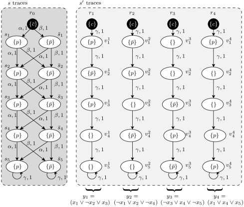
Figure 6: Example of mapping SAT to HyperPCTL model checking.

HyperPCTL formula: The HyperPCTL formula in our mapping is the following:

$$\varphi_{\mathsf{map}} = \exists\hat{\sigma}.\exists\hat{s}(\hat{\sigma}).\forall\hat{s}^{\prime}(\hat{\sigma}).\bar{c}_{\hat{s}(\hat{\sigma})}\,\wedge\,\bigg{(}c_{\hat{s}^{\prime}(\hat{\sigma})}\;\Rightarrow$$

$$\mathbb{P}\bigg{(}\operatorname{\leavevmode\hbox to8.7pt{\vbox to8.7pt{\text{[drawing]}}}}\Big{(}(p_{\hat{s}(\hat{\sigma})}\wedge p_{\hat{s}^{\prime}(\hat{\sigma})})\,\vee\,(\bar{p}_{\hat{s}(\hat{\sigma})}\wedge\bar{p}_{\hat{s}^{\prime}(\hat{\sigma})})\Big{)}\bigg{)}=1\bigg{)}$$

The intended meaning of the formula is that if there exists a scheduler that makes the formula true by choosing the $\alpha$ and $\beta$ actions, this scheduler gives us the assignment to the Boolean variables in the SAT instance. This is achieved by making all clauses true, hence, the $\forall\hat{s}^{\prime}(\hat{\sigma})$ subformula.

0.B.3 Reduction

We now show that the given SAT formula is satisfiable if and only if the MDP obtained by our mapping satisfies the HyperPCTL formula $\varphi_{\mathsf{map}}$.

($\Rightarrow$)

Suppose that $y$ is satisfiable. Then, there is an assignment that makes each clause $y_{j}$, where $j\in[1,m]$, true. We now use this assignment to instantiate a scheduler for the formula $\varphi_{\mathsf{map}}$. If $x_{i}=\mathtt{true}$, then we instantiate scheduler $\hat{\sigma}$ such that in state $s_{i-1}$ or $\bar{s}_{i-1}$, it chooses action $\alpha$. Likewise, if $x_{i}=\mathtt{false}$, then we instantiate scheduler $\hat{\sigma}$, such that in state $s_{i-1}$ or $\bar{s}_{i-1}$, it chooses action $\beta$. We now show that this scheduler instantiation evaluates formula $\varphi_{\mathsf{map}}$ to true. First observe that $\hat{s}(\hat{\sigma})$ can only be instantiate with state $r_{0}$ and $\hat{s}^{\prime}(\hat{\sigma})$ can only be instantiate with states $r_{j}$, where $j\in[1,m]$. Otherwise, the left side of the implication in $\varphi_{\mathsf{map}}$ becomes false, making the formula vacuously true. Since each $y_{j}$ is true, there is at least one literal in $y_{j}$ that is true. If this literal is of the form $x_{i}$, then we have $x_{i}=\mathtt{true}$ and the path that starts from $r_{0}$ will include $s_{i}$, which is labeled by $p$. Hence, the values of $p$, in both paths that start from $\hat{s}(\hat{\sigma})$ and $\hat{s}^{\prime}(\hat{\sigma})$ are eventually equal. If the literal in $y_{j}$ is of the form $\neg x_{i}$, then $x_{i}=\mathtt{false}$ and the path that starts from $\hat{s}(\hat{\sigma})$ will include $\bar{s}_{i}$. Again, the values of $\bar{p}$ are eventually equal. Finally, since all clauses are true, all paths that start from $\hat{s}^{\prime}(\hat{\sigma})$ reach a state where the right side of the implication becomes true.

($\Leftarrow$)

Suppose our mapped MDP satisfies formula $\varphi_{\mathsf{map}}$. This means that there exists a scheduler and state $\hat{s}(\hat{\sigma})$ that makes the subformula $\forall\hat{s}^{\prime}(\hat{\sigma})$ true, i.e., the path that starts from $r_{0}$ results in making the inner PCTL formula true for all paths that start from $r_{j}$. We obtain the truth assignment to the SAT problem as follows. If the scheduler chooses action $\alpha$ to state $s_{i}$, then we assign $x_{i}=\mathtt{true}$. Likewise, if the scheduler chooses action $\beta$ to state $\bar{s}_{i}$, then we assign $x_{i}=\mathtt{false}$. Observe that since in no state $p$ and $\bar{p}$ are simultaneously true and no path includes both $s_{i}$ and $\bar{s}_{i}$, variable $x_{i}$ will have only one truth value. Similar to the forward direction, it is straightforward to see that this valuation makes every clause $y_{j}$ of the SAT instance true.

And this concludes the proof. $~{}\blacksquare$

Appendix 0.C Proof of Theorem 5.2

Theorem. 5.2  Algorithm 1 returns a formula that is true iff its input HyperPCTL formula is satisfied by the input MDP.

Proof

The proof is by structural induction over the formula type. The cases for constants, atomic propositions, Boolean combinations and arithmetic expressions are straightforward. The remaining cases are the probabilistic temporal operators.

For the next-operator $\mathbb{P}(\operatorname{\leavevmode\hbox to7.41pt{\vbox to7.41pt{\text{[drawing]}}}}\varphi^{\prime})$ (line 2 in Algorithm 2), we first encode the meaning of the operand $\varphi^{\prime}$ (line 2); by induction assumption this encoding is sound. Since the operand is a state formula, its value is Boolean. The probability that the operand is true after one step is the sum of the probabilities to get to a state where the operand is true; we express this in pseudo-arithmetic by setting for each composed state $\vec{s}$ the value of $\textit{prob}_{\vec{s},\varphi^{\prime}}$ to $1$ if $\varphi^{\prime}$ holds there and to $0$ otherwise. Using these pseudo-Boolean values, we express for each composed state $\vec{s}=(s_{1},\ldots,s_{n})$ and each scheduler $\vec{\sigma}=(\sigma_{1},\ldots,\sigma_{n})$ the probability that $\varphi^{\prime}$ holds after one step by summing up for each possible successor $\vec{s}^{\prime}=(s_{1}^{\prime},\ldots,s_{n}^{\prime})$ the probability $\Pi_{i=1}^{n}\mathbf{P}(s_{i},\alpha_{i},s_{i}^{\prime})$ to get there in one step times the pseudo-Boolean value of $\textit{prob}_{\vec{s},\varphi^{\prime}}$ (lines 2–2).

The semantics of unbounded until $\mathbb{P}(\varphi_{1}\,\mathcal{U}\,\varphi_{2})$ is encoded in Algorithm 3. Similarly to the next-operator, we recursively encode the truth of the Boolean-valued operands (line 3). The remaining encoding follows for each composed state $\vec{s}$ and each scheduler $\vec{\sigma}=(\sigma_{1},\ldots,\sigma_{n})$ the standard fixedpoint-encoding of the probability to satisfy the until formula in the induced DTMC [20]. This probability is $1$ for all states satisfying $\varphi_{2}$ and $0$ for all states that do not satisfy any of the operands (line 3). Furthermore, the probability is also $0$ for all states from which no $\varphi_{2}$-states are reachable; we assure this by requiring for all positive probabilities the existence of a finite loop-free path to a $\varphi_{2}$-state using decreasing sequences of the arithmetic variables $d_{\vec{s},\varphi_{2}}$ (line 3). For all other cases, the encoding is similar to the next-operator, summing up for all possible successor states the probabilities to get there times the probability to satisfy the until formula along paths starting from there (line 3).

The case for unbounded until is a based on a technically rather complex case distinction, but it is just a direct encoding the semantics of bounded until.

References

• [1] Clarkson, M.R., Schneider, F.B.: Hyperproperties. Journal of Computer Security 18(6) (2010) 1157–1210
• [2] Alpern, B., Schneider, F.B.: Defining liveness. Information Processing Letters 21 (1985) 181–185
• [3] Goguen, J.A., Meseguer, J.: Security policies and security models. In: IEEE Symp. on Security and Privacy. (1982) 11–20
• [4] Zdancewic, S., Myers, A.C.: Observational determinism for concurrent program security. In: Proc. of CSFW’03. (2003)  29
• [5] Wang, Y., Zarei, M., Bonakdarpour, B., Pajic, M.: Statistical verification of hyperproperties for cyber-physical systems. ACM Transactions on Embedded Computing systems (TECS) 18(5s) (2019) 92:1–92:23
• [6] Bonakdarpour, B., Sánchez, C., Schneider, G.: Monitoring hyperproperties by combining static analysis and runtime verification. In: Proc. of ISoLA’18. (2018) 8–27
• [7] Ábrahám, E., Bonakdarpour, B.: HyperPCTL: A temporal logic for probabilistic hyperproperties. In: Proc. of QEST’18. (2018) 20–35
• [8] Ábrahám, E., Bartocci, E., Bonakdarpour, B., Dobe, O.: Parameter synthesis for probabilistic hyperproperties. In: Proc. of LPAR-23: the 23rd International Conference on Logic for Programming, Artificial Intelligence and Reasoning. Volume 73 of EPiC Series in Computing., EasyChair (2020) 12–31
• [9] Wang, Y., Nalluri, S., Bonakdarpour, B., Pajic, M.: Statistical model checking for hyperproperties. In: Proceedings of the IEEE 34th Computer Security Foundations (CSF). (2021) To appear.
• [10] Guarnieri, M., Marinovic, S., Basin, D.: Securing databases from probabilistic inference. In: Proc. of CSF’17. (2017) 343–359
• [11] Dimitrova, R., Finkbeiner, B., Torfah, H.: Probabilistic hyperproperties of markov decision processes. In: Proceedings of the 18th Symposium on Automated Technology for Verification and Analysis (ATVA). (2020) To appear.
• [12] Baier, C., Brázdil, T., Größer, M., Kucera, A.: Stochastic game logic. Acta Informatica 49(4) (2012) 203–224
• [13] Ngo, T.M., Stoelinga, M., Huisman, M.: Confidentiality for probabilistic multi-threaded programs and its verification. In: Proc. of ESSoS’13. (2013) 107–122
• [14] Knuth, D., Yao, A.: The complexity of nonuniform random number generation. In: Algorithms and Complexity: New Directions and Recent Results. Academic Press (1976)
• [15] : STORMPY. https://moves-rwth.github.io/stormpy/
• [16] Dehnert, C., Junges, S., Katoen, J., Volk, M.: A Storm is coming: A modern probabilistic model checker. In: Proc. of CAV’17. (2017) 592–600
• [17] de Moura, L.M., Bjørner, N.: Z3: An efficient SMT solver. In: Proc. of TACAS’08. (2008) 337–340
• [18] Baier, C., Bertrand, N., Größer, M.: On decision problems for probabilistic Büchi automata. In: Proc. of FOSSACS’08. (2008) 287–301
• [19] Bonakdarpour, B., Finkbeiner, B.: The complexity of monitoring hyperproperties. In: Proc. of CSF’18. (2018) 162–174
• [20] Baier, C., Katoen, J.P.: Principles of Model Checking. The MIT Press (2008)