Stochastic Properties of Static Friction

Abstract

The onset of frictional motion is mediated by rupture-like slip fronts, which nucleate locally and propagate eventually along the entire interface causing global sliding. The static friction coefficient is a macroscopic measure of the applied force at this particular instant when the frictional interface loses stability. However, experimental studies are known to present important scatter in the measurement of static friction; the origin of which remains unexplained. Here, we study the nucleation of local slip at interfaces with slip-weakening friction of random strength and analyze the resulting variability in the measured global strength. Using numerical simulations that solve the elastodynamic equations, we observe that multiple slip patches nucleate simultaneously, many of which are stable and grow only slowly, but one reaches a critical length and starts propagating dynamically. We show that a theoretical criterion based on a static equilibrium solution predicts quantitatively well the onset of frictional sliding. We develop a Monte-Carlo model by adapting the theoretical criterion and pre-computing modal convolution terms, which enables us to run efficiently a large number of samples and to study variability in global strength distribution caused by the stochastic properties of local frictional strength. The results demonstrate that an increasing spatial correlation length on the interface, representing geometric imperfections and roughness, causes lower global static friction. Conversely, smaller correlation length increases the macroscopic strength while its variability decreases. We further show that randomness in local friction properties is insufficient for the existence of systematic precursory slip events. Random or systematic non-uniformity in the driving force, such as potential energy or stress drop, is required for arrested slip fronts. Our model and observations provide a necessary framework for efficient stochastic analysis of macroscopic frictional strength and establish a fundamental basis for probabilistic design criteria for static friction.

1 Introduction

Static friction is the maximal shear load that can be applied to an interface between two solids before they start to slide over each other. The famous Coulomb friction law (Amontons, 1699; Coulomb, 1785; Popova and Popov, 2015) states that static friction is proportional to the normal load with the friction coefficient being the proportionality factor. The friction coefficient is generally reported as function of the contacting material pair, which is often misinterpreted as the friction coefficient being a material (pair) property. While proportionality of friction to normal load is mostly valid, the friction coefficient is geometry-dependent and thus varies for different experimental setups with the same material pair (Ben-David and Fineberg, 2011). The underlying cause for this observation is the mechanism governing the onset of frictional sliding, which has been shown to be a fracture-like phenomenon (Svetlizky and Fineberg, 2014; Svetlizky et al., 2020; Rubino et al., 2017). The geometry and deformability of the solids lead to a non-uniform stress state along the interface. As a consequence, local frictional strength is reached at a critical point and slip nucleation starts, from where it extends in the space-time domain – just like a crack – until the entire interface transitioned and global sliding occurs.

Variations in the static friction force, however, do not only occur because of changes in the loading configuration. Experiments have shown that the measured friction force varies also from one experiment to another when the exact same setup and exact same specimens are used. For instance, Rabinowicz (1992) showed that the static friction coefficient of a gold-gold interface, measured by a tilting plane friction apparatus, varies from $0.32$ to $0.80$ for normal load $75~{}\mathrm{g}$. Similar but to a lesser extent, Ben-David and Fineberg (2011) also observed variations in the static friction coefficient of glassy polymers when the loading configuration was fixed.

While these variations are not often reported, they are an important factor in the absence of a complete and consistent theory for friction (Spencer and Tysoe, 2015). If (seemingly) equivalent experiments lead to a large range of observations without consistent trends, it is challenging to isolate the relevant from the irrelevant contributions and, therefore, nearly impossible to create a fundamental understanding of the underlying process. Even though the presence of these large variations has important implications for the study of friction, current knowledge about the origin and properties of these observed variations in macroscopic friction remains limited.

One possible origin is randomness in local friction properties. Interfaces have been shown to consist of an ensemble of discrete micro-contacts (Bowden and Tabor, 1950; Dieterich and Kilgore, 1994; Sahli et al., 2018), which are created by surface roughness (Thomas, 1999; Hinkle et al., 2020) when two solids are brought into contact. This naturally leads to a system with random character, where micro-contacts of random size are distributed randomly along the interface (Greenwood et al., 1966; Persson, 2001; Hyun and Robbins, 2007; Yastrebov et al., 2015). Since frictional strength is directly related to the cumulative contact area of theses micro-contacts (Bowden and Tabor, 1950; Greenwood et al., 1966), and the micro-contacts are the result of random surface roughness, the local frictional strength is likely also random.

Surprisingly, the effect of interfacial randomness on friction remains largely unexplored. Most of previous work is focused on how (random) surface roughness is related to various friction phenomenology including rate-dependence (Li et al., 2013; Lyashenko et al., 2013), local pressure excursions within lubricated contact (Savio et al., 2016), chemical aging (Li et al., 2018), or the existence of static friction (Sokoloff, 2001). How interfacial randomness causes variation in these observations has, however, not been studied so far. Only most recently, Amon et al. (2017) and Geus et al. (2019) have considered variability in friction. Amon et al. (2017) showed that systems with a nonuniform initial stress state with long range coupling are characterized by two regimes: at low loading, small patches of the system undergo sliding in an uncorrelated fashion; at higher loading, instabilities occur at regular intervals over patches of increasing size – just like confined stick-slip events (Kammer et al., 2015; Bayart et al., 2016) – and eventually span the whole system. Geus et al. (2019) simulated interface asperities as an elasto-plastic continuum with randomness in its potential energy and show that the stress drop during a stick-slip cycle is a stochastic property which vanishes with increasing number of asperities. These results demonstrate well the stochastic character of macroscopic friction due to random interface properties. However, the effects of interfacial randomness on the variability of macroscopic static friction, e.g., the friction coefficient, has not been studied yet.

Here, we address this gap of knowledge and aim at a better understanding of the stochastic properties of static friction. We present a combined numerical and theoretical study that links randomness of local friction properties with observed variability in macroscopic strength. Using dynamic simulations, we will show that the macroscopic friction threshold is attained when a local slipping area, of which many can co-exist, reaches a critical length and nucleates the onset of friction. This nucleation patch becomes unstable and propagates across the entire interface causing global sliding. We will then show that a quasi-static equilibrium theory, which takes an integral form, predicts quantitatively well the critical stress level that causes nucleation of global sliding. Based on this theoretical model, we will develop fast and accurate Monte Carlo simulations using a Fourier representation of the integral equations, and demonstrate the extent of variability in macroscopic static friction based on random interface strength with various correlation lengths. Finally, we will show that a decreasing interfacial correlation length leads to higher macroscopic strength with decreased variability.

This paper is structured as follows. First, we provide a problem statement in Sec. 2 including a description of the physical system, the stochastic properties, and our approach to generate random strength fields. In Sec. 3, we present the numerical method used to simulate the onset of frictional sliding and compare simulation results of critical stress leading to global sliding with predictions based on a theoretical model. This model is then used in an analytical Monte Carlo study, which is developed and presented in Sec. 4. The implications of our model assumptions as well as the model results are discussed in Sec. 5. Finally, we provide a conclusion in Sec. 6.

2 Problem Statement

In this section, we first provide a description of the physical problem that we consider throughout this paper. We then describe the stochastic properties of the strength profile along the interface and, finally, explain how we generate these random fields.

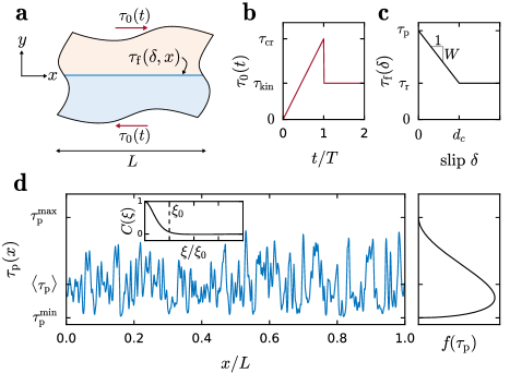
Figure 1: Problem statement. (a) A frictional interface (blue line) of strength $\tau_{\mathrm{f}}(\delta,x)$ embedded within two semi-infinite elastic solids, which are periodic in $x$ with period $L$ and infinite in $y$. A uniform loading $\tau_{0}(t)$ is applied. (b) $\tau_{0}(t)$ is increased linearly with time $t$ up to the onset of frictional motion when the stress drops from its critical value $\tau_{\mathrm{cr}}$ to a kinetic level $\tau_{\mathrm{kin}}$. (c) The constitutive relation of the frictional interface is a linear slip-weakening law $\tau_{\mathrm{f}}(\delta)$ with random peak strength $\tau_{\mathrm{p}}(x)$ and constant weakening rate $W$ (see Eq. 1). (d) $\tau_{\mathrm{p}}(x)$ is a random field with spatial correlation $C(\xi)$ (inset) and probability density function $f(\tau_{\mathrm{p}})$ (right).

2.1 Physical Problem

We study the macroscopic strength of a frictional interface. Our objective is to provide a fundamental understanding of the effect of local variations in frictional strength on the macroscopic response. For this reason, we focus on the simplest possible problem – without oversimplifying the constitutive relations of the bulk and the interface. Specifically, we consider a two-dimensional (2D) system consisting of two semi-infinite elastic solids, as shown in Fig. 1a. The domain is infinite in the $y$ direction and periodic in $x$ with period $L$. Both materials have the same elastic properties.

We apply a uniform shear load $\tau_{0}(t)$ that increases quasi-statically with time (see Fig. 1b). Once $\tau_{0}(t)$ reaches the macroscopic strength of the interface $\tau_{\mathrm{cr}}$, the interface starts to slide and the frictional strength suddenly reduces to its kinetic level $\tau_{\mathrm{kin}}$. This observed reduction in shear stress is typically associated with friction-weakening processes, which may depend on various properties, such as slip, slip rate, and interface state. The critical shear stress $\tau_{\mathrm{cr}}$, if divided by the contact pressure, corresponds to the static macroscopic friction coefficient. Similarly, $\tau_{\mathrm{kin}}$ is proportional to the kinetic friction coefficient.

These macroscopic observations depend on the local interface properties, which are the peak strength $\tau_{\mathrm{p}}(x)$, and residual strength $\tau_{\mathrm{r}}(x)$. As we will show, the local properties are generally different from the macroscopic properties; particularly, in the case of non-uniform stress or strength. For simplicity, we describe the evolution of the local frictional strength as a linear slip-weakening law, which is shown in Fig. 1c and is given by

$$\tau_{\mathrm{f}}(\delta)=\tau_{\mathrm{r}}+W(d_{\mathrm{c}}-\delta)H(d_{\mathrm{c}}-\delta)~{},$$ (1)

where $\delta(x)$ is local slip, $d_{\mathrm{c}}(x)$ is a characteristic length scale, and $W(x)=(\tau_{\mathrm{p}}(x)-\tau_{\mathrm{r}}(x))/d_{\mathrm{c}}(x)$ is the weakening rate. $H(.)$ is the Heaviside function.

We consider a heterogeneous system with local peak strength $\tau_{\mathrm{p}}(x)$ being a random field, as further described in Sec. 2.2. To reduce complexity of the problem, we assume uniform residual strength $\partial_{x}\tau_{\mathrm{r}}=0$ and uniform weakening rate $\partial_{x}W=0$. The variation in local peak strength is thought to represent possible heterogeneity in the material, but also the effect of surface roughness, which leads to a real contact area that consists of an ensemble of discrete contact points with varying properties. The implications of this approach will be discussed in depth in Sec. 5.

2.2 Stochastic Properties of Frictional Interface

The local peak strength $\tau_{\mathrm{p}}(x)$ is modeled as a stationary non-Gaussian random field with specified cumulative distribution function $F(\tau_{\mathrm{p}})$ and corresponding probability density $f(\tau_{\mathrm{p}})$, as shown in Fig. 1d. The random field is defined by the nonlinear mapping

$$\tau_{\mathrm{p}}(x)=F^{-1}\Big{(}{\Phi\big{(}z(x)\big{)}}\Big{)}~{},$$ (2)

where $z(x)$ is Gaussian with zero mean and unit variance and $\Phi$ its cumulative distribution, depicted in Fig. 2a-left. $F$ and $\Phi$ are monotonic by definition, so their inverse exist, which can be used to prove that $P\left(\tau_{\mathrm{p}}(x)\leq\tau\right)=F(\tau)$. Further, with $\tau_{\mathrm{p}}$ being the local peak strength of the interface, it needs to satisfy some physical requirements. First, the peak strength is always higher than the residual strength, i.e., $\tau_{\mathrm{p}}^{\min}\geq\tau_{\mathrm{r}}$. Second, it maximum value is limited by the material properties. For this reason, we require that $\tau_{\mathrm{p}}\in(\tau_{\mathrm{p}}^{\min},\tau_{\mathrm{p}}^{\max})$, which we achieve by setting $F(\tau_{\mathrm{p}})$ as a Beta cumulative distribution function (see Fig. 2a-right).

The spatial evolution of $z(x)$ is specified by its power spectral density $g(k)$, which corresponds to the Fourier transform of the correlation function $C_{z}(\xi)$, i.e.,

$$g(k)\equiv\int_{-\infty}^{+\infty}C_{z}(\xi)e^{-ik\xi}\mathrm{d}\xi~{},$$ (3)

where $k$ is the angular wave number. We assume that $z(x)$ has a power spectral density

$$g(k)\propto{(k^{2}+\lambda^{2})^{-4}}~{},$$ (4)

where $\lambda$ is the cutoff frequency, above which the spectral density decays as a power law $\sim k^{-8}$ (see Fig. 2b). The correlation length $\xi_{0}$ is a measure of memory of the random field; the longer $\xi_{0}$ the longer the memory. $\xi_{0}$ is inversely proportional to $\lambda$, and we define it as $\xi_{0}=2\pi/\lambda$. Since the correlation function of $z$ is positive, $C_{z}(\xi)>0$, it is not greatly affected by the nonlinear mapping $F^{-1}\circ\Phi$ and $C_{z}(\xi)\approx C_{\tau_{\mathrm{p}}}(\xi)$ (Grigoriu, 1995, p.48) and features such as $\xi_{0}$ are preserved (see Fig. 1.d inset). The assumption of using this specific spectral density and probability distribution are discussed in Sec. 5.3.

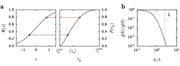
Figure 2: Stochastic properties of the random peak strength field $\tau_{\mathrm{p}}(x)$. (a) The random variable $\tau_{\mathrm{p}}$ is generated by applying a nonlinear mapping $F^{-1}\circ\Phi(x)$ (Eq. 2) onto the Gaussian random variable $z$. Two colored dots inked by a line represent a $(z,\tau_{\mathrm{p}})$ pair with equal cumulative density $F(\tau_{\mathrm{p}})=\Phi(z)$, which is the criterion imposed by the nonlinear mapping. (b) Normalized spectral density function $g(k)/g(0)$ (Eq. 4). $\bar{k}$ is the truncation frequency and $\lambda=2\pi/\xi_{0}$ is the cutoff frequency.

2.3 Random Field Samples Generation

The samples of random field $\tau_{\mathrm{p}}(x)$ are generated as follows. First, the Gaussian random field $z(x)$ is generated using a spectral representation

$$z(x)=\sum_{j=1}^{J}\sigma_{j}\left(A_{j}\cos(k_{j}x)+B_{j}\sin(k_{j}x)\right),$$ (5)

where $A_{j}$ and $B_{j}$ are independent Gaussian random variables with zero mean and unit variance and modal angular wave-number is $k_{j}=2\pi j/L$. The fundamental wavelength of the field $2\pi/k_{1}=L$ is chosen such that it corresponds to the domain size $L$, which implies that $z(x)$ is periodic over $L$, and so is $\tau_{p}(x)$. The modal variance $\sigma_{j}^{2}\propto g(k_{j})$ corresponds to the discrete spectral density, which is normalized to assure that $z$ has unit variance

$$\sigma_{j}^{2}={\frac{g(k_{j})}{\sum_{j=1}^{J}g(k_{j})}}.$$ (6)

Due to the discrete representation of $z(x)$, we apply a truncation frequency that is considerably larger than the cutoff frequency $\bar{k}\equiv k_{J}=2.5\lambda$. This ensures that most of the spectral power is preserved:

$$\frac{\int_{0}^{\bar{k}}g(k)\mathrm{d}k}{\int_{0}^{\infty}g(k)\mathrm{d}k}\approx 0.9997$$ (7)

Further increase in $\bar{k}$ would include additional high frequency modes but with negligible amplitudes. Finally, once $z(x)$ has been generated, we apply the nonlinear mapping $F^{-1}\circ\Phi$ (Eq. 2 and visualized in Fig. 2a) and obtain the random field $\tau_{\mathrm{p}}(x)$. Fig. 1d shows a sample of $\tau_{\mathrm{p}}(x)$ generated using the described procedure with corresponding correlation function and probability density.

3 Dynamic Simulations

In the following, we will first present the numerical method and model setup applied in our simulations of the onset of friction. We then provide a theoretical model to describe the simulations and present a comparison between the theoretical predictions with the numerical results.

3.1 Numerical Method

We model the physical problem, as described in Sec. 2.1, with the Spectral Boundary Integral Method (SBIM) (Geubelle and Rice, 1995; Breitenfeld and Geubelle, 1998). This method solves efficiently and precisely the elasto-dynamic equations of each half space. The spectral formulation applied in SBIM naturally provides periodicity along the interface. The half spaces are perfectly elastic and we apply a shear modulus of $G=1~{}\mathrm{GPa}$, Poisson’s ratio of $\nu=0.33$ and density $\rho=1170~{}\mathrm{kg/m}^{3}$, and impose a plane-stress assumption. While we will report our results in adimensional quantities, we note that these parameters correspond to the static properties of glassy polymers, which have been widely used for friction experiments (Svetlizky and Fineberg, 2014; Rubino et al., 2017).

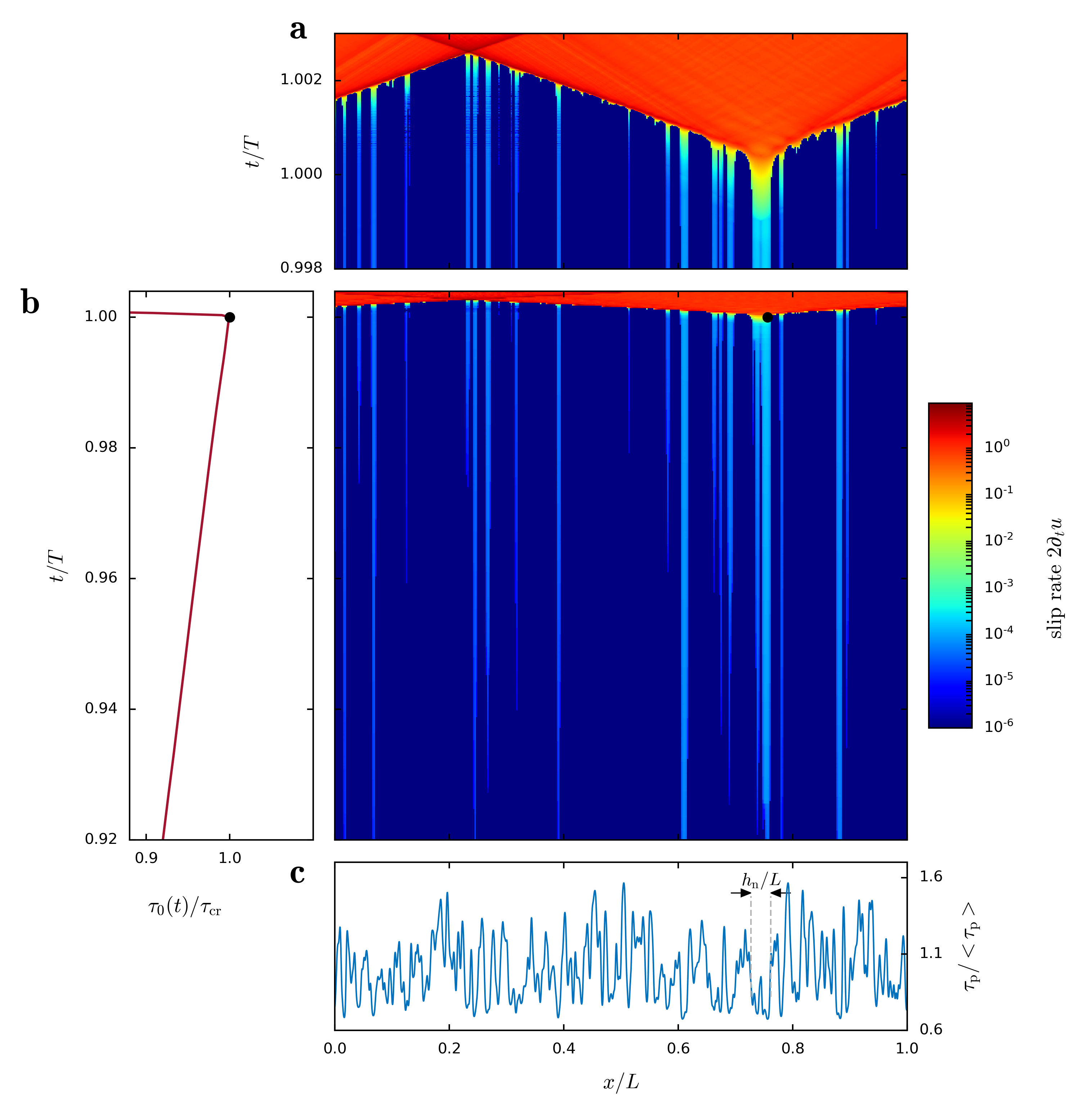
Figure 3: Representative numerical simulation of the onset of frictional sliding along an interface with random peak strength. (a) Space-time diagram of slip rate along the interface. Time is normalized by the time of friction onset $T$. Nucleation occurs at $x/L\approx 0.75$. (b-right) Same space-time diagram as in (a) with larger time span. Nucleation is marked by a black dot at $x/L\approx 0.75$ and $t/T=1$. (b-left) Evolution of applied load $\tau_{0}(t)$ normalized by its maximum value $\tau_{\mathrm{cr}}$. This corresponds to Fig. 1b. (c) Random profile of peak strength $\tau_{\mathrm{p}}(x)$ for simulation shown in (a-b). The correlation length is $\xi_{0}/h_{\mathrm{n}}=0.25$. The size of the critical nucleation patch $h_{\mathrm{n}}$ is marked by black arrows.

The interface between the two half spaces is coupled by a friction law as given by Eq. 1. The friction law corresponds essentially to a cohesive law, as known from fracture-mechanics simulations, but applied to the tangential direction. It describes the evolution of local strength as a function of slip. We apply peak strength $\tau_{\mathrm{p}}(x)$ as a random field, following the description provided in Sec. 2.2, and constant $\tau_{\mathrm{r}}$. $\tau_{\mathrm{p}}(x)$ follows a Beta distribution with $\alpha=1.5$ and $\beta=3$. We impose a maximum value for relative peak strength of $\max(\tau_{\mathrm{p}}(x)-\tau_{\mathrm{r}})=1.66~{}\mathrm{MPa}$ and minimum value of $\min(\tau_{\mathrm{p}}(x)-\tau_{\mathrm{r}})=0.66~{}\mathrm{MPa}$. Therefore, the random field has a mean value of $\left<\tau_{\mathrm{p}}-\tau_{\mathrm{r}}\right>=1~{}\mathrm{MPa}$ and standard deviation of $0.2~{}\mathrm{MPa}$. We further apply a constant slip-weakening rate of $W=0.5~{}\mathrm{TPa/m}$, which is representative for glassy polymers (Svetlizky et al., 2020). Finally, a slowly increasing uniform stress $\tau_{0}(t)$ is applied along the entire interface.

We use a repetition length of $L=0.1~{}\mathrm{m}$, which is, as we will show, considerably larger than the characteristic nucleation length scale. The interface is discretized by $512-1024$ nodes. We verified convergence with respect to discretization, loading rate, and time step.

The results of a representative simulation are shown in Fig. 3. The $\tau_{\mathrm{p}}(x)$ profile has many local minima (see Fig. 3c). Depending on their value, these minima cause localized slip, as evidenced by bright blue vertical stripes over most of the time period shown in Fig. 3b-right. These localized slip patches grow slowly with increasing loading, which is difficult to see for most patches in Fig. 3b-right. Growth is easiest observed for the slip patch at $x/L\approx 0.75$. Incidentally, this patch grows enough to reach a critical size from which on the patch becomes unstable, marked by a black dot, and starts growing dynamically. This dynamic propagation, see orange-red area in Fig. 3a enlarged from Fig. 3b-right, does not stop and, therefore, causes sliding along the entire interface – hence global sliding. The effect on the macroscopic applied force is shown in Fig. 3b-left, where $\tau_{0}(t)=\int_{L}\tau(x,t)\mathrm{d}x$. At the precise moment when the slip patch becomes unstable, marked by a black dot, $\tau_{0}(t)$ starts decreasing rapidly. The maximum value, denoted $\tau_{\mathrm{cr}}$, represents the macroscopic strength of the interface.

The simulation shows that macroscopic strength is not reached when the first point along the interface starts sliding but when the most critical slip patch becomes unstable, starts propagating dynamically, and ”breaks” the entire interface. Therefore, the criterion determining macroscopic strength is non-local and depends on the stability of local slip patches. In the following section, we will present a theoretical description of this nucleation process and provide a criterion for the limit of macroscopic strength.

3.2 Theory for Nucleation of Local Sliding

During the nucleation process, a weak point along the interface starts sliding. Due to local stress transfer, the size of this slipping area grows continuously until it reaches a critical size and unstable interface sliding occurs (Campillo and Ionescu, 1997). In this section, we will adapt the criterion developed by Uenishi and Rice (2003), which is shortly summarized in A, to describe and predict the limits of stable slip-area growth. Uenishi and Rice (2003) considered a similar system with two main differences to the problem studied here. First, in their case, the interface strength is uniform and the applied load is non-uniform. A shows that both problems result in the same equation for the problem statement and thus lead to the same nucleation criterion. Second, Uenishi and Rice (2003) considered a system with an isolated non-uniformity in the applied load. In other words, the applied stress was mostly uniform but with one well-contained local increase. Therefore, the location of nucleation is known in advanced. In our system, where the non-uniform property is random, the location is unknown. We will address this difference here and discuss it further in Sec. 5.

Uenishi and Rice (2003) showed that on interfaces governed by linear slip-weakening friction (Eq.1), there is a unique critical length for stable growth of the slipping area, which can be approximated by

$$h_{\mathrm{n}}\approx 1.158\frac{G^{*}}{W}~{},$$ (8)

where $G^{*}=G/(1-\nu)$ for mode II plane-stress ruptures, assuming the stress within $h_{\mathrm{n}}$ has not attained the residual value $\tau_{\mathrm{r}}$ anywhere. Eq. 8 shows that $h_{\mathrm{n}}$ depends only on the shear modulus $G^{*}$ and the slip-weakening rate $W$. Most importantly, the critical length is independent of the shape of the non-uniformity in the system. Specifically to our case, it does not depend on the functional form of $\tau_{\mathrm{p}}(x)$. Since we have homogeneous elastic solids and a uniform slip-weakening rate $W$, the critical size $h_{\mathrm{n}}$ is unique and uniform along the entire interface.

The important question for our problem, however, is to determine the level of critical stress that causes a nucleation patch to reach $h_{\mathrm{n}}$ and initiate global sliding. The solution for the stress level leading to nucleation, as derived by Uenishi and Rice (2003), is given by Eq. 21, and can be rewritten in terms of $\tau_{\mathrm{p}}(x)$ and $h_{\mathrm{n}}$ as

$$\tau_{\mathrm{n}}(x)\approx 0.751\int_{-1}^{+1}\tau_{\mathrm{p}}\left(\frac{h_{\mathrm{n}}}{2}s+x\right)~{}v_{0}(s)~{}\mathrm{d}s~{},$$ (9)

where $x$ is the center location of the nucleation patch and $v_{0}(s)\approx(0.925-0.308s^{2})\sqrt{1-s^{2}}$ is the first eigenfunction of the elastic problem. Note that the transformation applied to the argument of $\tau_{\mathrm{p}}(x)$ results in the integral being computed over the critical nucleation patch size $h_{\mathrm{n}}$. Eq. 9 shows that the nucleation stress, which leads to a nucleation patch of size $h_{\mathrm{n}}$, does clearly depend on the shape of $\tau_{\mathrm{p}}(x)$. Note that Eq. 9 assumes that stresses within the nucleation patch have not attained the residual strength yet i.e., the fracture process zone spans the entire crack. In this case, the assumption of small-scale yielding does not hold, and, thus, the Griffith criterion for crack propagation does not apply.

As stated earlier, the nucleation stress $\tau_{\mathrm{n}}(x)$ was derived for a contained non-uniformity, for which we know the location. Therefore, $\tau_{\mathrm{n}}(x)$ corresponds to the critical stress of the system. In our system, however, $\tau_{\mathrm{p}}(x)$ is random and multiple nucleation patches might slowly grow. Determining the critical stress $\tau_{\mathrm{cr}}$ of the system requires computing the nucleation stress $\tau_{\mathrm{n}}$ for each nucleation patch and identifying the critical one. To address this aspect, we propose to compute Eq. 9 as a weighted moving average over the entire interface, and define the critical stress to be its minimum (see Fig. 4a). Therefore, we define the critical stress $\tau_{\mathrm{cr}}$ as

$$\tau_{\mathrm{cr}}=\tau_{\mathrm{n}}(x_{\mathrm{cr}})\quad\mathrm{such~{}that}~{}\tau_{\mathrm{cr}}<\tau_{\mathrm{n}}(x)\quad\forall x\neq x_{\mathrm{cr}}~{}.$$ (10)

For simplicity, we refer to this definition also as $\tau_{\mathrm{cr}}=\min(\tau_{\mathrm{n}}(x))$ and $x_{\mathrm{cr}}=\mathrm{arg}\min(\tau_{\mathrm{n}}(x))$. While it is possible, but not very likely, to have multiple minima of $\tau_{\mathrm{n}}$ with the same amplitude, this does not affect the resulting $\tau_{\mathrm{cr}}$. However, multiple $x_{\mathrm{cr}}$ could coexist which would result in multiple slip patches becoming unstable simultaneously. By adopting Eq. 9 and defining Eq. 10, we essentially assume that there is no interaction between nucleation patches. We will verify the validity of this assumption in the following section.

3.3 Results

We compare the results from numerical simulations, as described in Sec. 3.1, with the theoretical prediction from Sec. 3.2 by analyzing simulations with random $\tau_{\mathrm{p}}(x)$ generated using the method described in Sec. 2.3. For each of the three different correlation lengths $\xi_{0}/h_{\mathrm{n}}=0.25$, $0.5$, and $2.0$ we run $20$ simulations. The system size is fixed and chosen such that it is considerably larger than the nucleation length, i.e., $h_{\mathrm{n}}/L=0.034$.

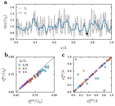
Figure 4: Verification of nucleation criterion on numerical simulations. (a) The random profile of $\tau_{\mathrm{p}}(x)$ from simulation shown in Fig. 3 is depicted by dashed gray line. The nucleation stress $\tau_{\mathrm{n}}(x)$ computed from $\tau_{\mathrm{p}}(x)$ by Eq. 9 is shown as solid blue line. The point of nucleation given by Eq. 10, i.e., ($x_{\mathrm{cr}}$,$\tau_{\mathrm{cr}}$), is marked by a black dot. (b) Comparison of critical length from theoretical prediction by Eq. 10 $\tau_{\mathrm{cr}}^{\mathrm{pred}}$ as shown in (a) with values measured from numerical simulations $\tau_{\mathrm{cr}}^{\mathrm{sim}}$ as illustrated in Fig. 3. $20$ simulations are computed for each $\xi_{0}/h_{\mathrm{n}}$ value. (c) Comparison of nucleation location from theoretical prediction $x_{\mathrm{cr}}^{\mathrm{pred}}$ with simulation result $x_{\mathrm{cr}}^{\mathrm{sim}}$ for the same $60$ simulations as shown in (b). (b-c) Gray line indicates slope of $1$.

A representative example is shown in Fig. 3. The size of $h_{\mathrm{n}}/L$ is indicated in Fig. 3c and appears to provide a reasonable prediction for the nucleation patch size as observed in Fig. 3a. Further comparison is given in Fig. 4a. First, we illustrate the theoretical prediction. The nucleation stress $\tau_{\mathrm{n}}(x)$ (solid blue line) is computed from $\tau_{\mathrm{p}}(x)$ (gray dashed line) using Eq. 9, and $\tau_{\mathrm{cr}}$ is, according to Eq. 10, the minimum of $\tau_{\mathrm{n}}(x)$ (marked by black dot). We find the location of nucleation to be $x_{\mathrm{cr}}/L\approx 0.75$, which corresponds to our observation from the numerical simulation, as seen in Fig. 3.

A more precise and systematic comparison is provided in Fig. 4b&c. We compare the predicted critical stress $\tau_{\mathrm{cr}}^{\mathrm{pred}}$ with the measured value from dynamic simulations $\tau_{\mathrm{cr}}^{\mathrm{sim}}$. We compute $\tau_{\mathrm{cr}}^{\mathrm{pred}}$ as described above with Eq. 10, and as illustrated in Fig. 4a. We further find $\tau_{\mathrm{cr}}^{\mathrm{sim}}=T\partial_{t}\tau_{0}$, where $\partial_{t}\tau_{0}$ is the applied loading rate and $T$ is the time at which $\tau_{0}(t)$ is maximal (see Fig. 3b-left). Comparison of $\tau_{\mathrm{cr}}^{\mathrm{pred}}$ with $\tau_{\mathrm{cr}}^{\mathrm{sim}}$ is shown in Fig. 4b for all $60$ simulations. The results show that the prediction works generally well. For decreasing $\xi_{0}/h_{\mathrm{n}}$ the prediction becomes slightly less accurate with a tendency to over-predict the critical value. The results further show that the predicted and measured critical stress $\tau_{\mathrm{cr}}$ increases with decreasing $\xi_{0}/h_{\mathrm{n}}$.

While the location of nucleation is not relevant for the apparent global strength of our system, we compare the predicted and simulated $x_{\mathrm{cr}}$ for further evaluation of the developed theory. The comparison shown in Fig. 4c uses $x_{\mathrm{cr}}^{\mathrm{pred}}$, as given by Eq. 10 and shown for an example in Fig. 4a, and $x_{\mathrm{cr}}^{\mathrm{sim}}$ as found by analyzing the simulation data as illustrated in Fig. 3a&b-right. The data shows that the prediction works well for most of the simulations. For $8$ simulations, $6$ of which have $\xi_{0}/h_{\mathrm{n}}=0.25$, the prediction does not work. However, as shown in Fig. 4b, $\tau_{\mathrm{cr}}$, which is the quantity of interest here, is correctly predicted for all of these cases. The reason for this discrepancies are likely second-order effects, as we will discuss in Sec. 5.

Overall, the results show that $\tau_{\mathrm{cr}}$ is quantitatively well predicted by the theory presented in Sec. 3.2. This allows us to study systematically the effect of randomness in interface properties by applying the theoretical model in analytical Monte Carlo simulations.

4 Analytical Monte Carlo Study

In the following section, we introduce Monte Carlo simulations, which are based on the theoretical framework for nucleation of frictional ruptures in a random field of frictional strength $\tau_{\mathrm{p}}(x)$, as derived in Sec. 3.2. The effect of correlation length $\xi_{0}$ on the effective frictional strength $\tau_{\mathrm{cr}}$ (Eq. 10), and its probability distribution $f(\tau_{\mathrm{cr}})$, is studied, while keeping all other properties constant. A Monte Carlo study based on the full dynamic problem (Sec. 3.1) would be computationally daunting. However, the theoretical framework allows us to evaluate $\tau_{\mathrm{cr}}$ very efficiently and has been validated by 20 full dynamic simulations for each considered $\xi_{0}$ (see Fig. 4).

4.1 Monte Carlo Methodology

The effective frictional strength $\tau_{\mathrm{cr}}=\min(\tau_{\mathrm{n}}(x))$ requires the computation of the nucleation strength $\tau_{\mathrm{n}}(x)$, which involves a convolution of the local peak strength $\tau_{\mathrm{p}}(x)$ with the eigenfunction $v_{0}$, given in Eq. 9. Considerable computation time can be saved by using a spectral representation of the random field $\tau_{\mathrm{p}}(x)$:

$$\tilde{\tau}_{\mathrm{p}}(x)=\sum_{j=0}^{J}\hat{\tau}_{\mathrm{p}}(k_{j})e^{-ik_{j}x},$$ (11)

where $\tilde{}$ signifies that $\tilde{\tau}_{\mathrm{p}}(x)$ is an approximation of $\tau_{\mathrm{p}}(x)$ and the number of frequencies $J$ is chosen such that the approximation error $|\tilde{\tau}_{\mathrm{p}}-\tau_{\mathrm{p}}|$ is negligible. $\hat{\tau}_{\mathrm{p}}(k_{j})$ is the discrete Fourier transform of $\tau_{\mathrm{p}}(x)$

$$\hat{\tau}_{\mathrm{p}}(k_{j})=\int_{0}^{L}\tau_{\mathrm{p}}(x)e^{-ik_{j}x}\mathrm{d}x,$$ (12)

where $\tau_{\mathrm{p}}(x)$ is generated using the procedure described in Sec. 2.3. By substituting Eq. 11 into Eq. 9 the nucleation strength convolution becomes a dot product:

$$\begin{split}\tilde{\tau}_{\mathrm{n}}(x)&\approx 0.751\int_{-1}^{+1}\sum_{j=0}^{J}\hat{\tau}_{\mathrm{p}}(k_{j})e^{-ik_{j}\left(s~{}h_{\mathrm{n}}/2+x\right)}v_{0}(s)\mathrm{d}s\\ &\approx 0.751\sum_{j=0}^{J}\hat{\tau}_{\mathrm{p}}(k_{j})g_{j}(x)\end{split}$$ (13)

where $g_{j}(x)=\int_{-1}^{+1}e^{-ik_{j}\left(\frac{h_{\mathrm{n}}}{2}s+x\right)}v_{0}(s)\mathrm{d}s$ is the modal convolution term, which, being independent of the sample specific functional form of $\tau_{\mathrm{p}}(x)$, can be pre-computed. This formulation allows for efficient and precise evaluation of the effective frictional strength $\tau_{\mathrm{cr}}=\min\tau_{\mathrm{n}}(x)$ for a large number of samples $N=10,000$, such that the probability distribution $f(\tau_{\mathrm{cr}})$ and its evolution as function of the correlation length $\xi_{0}$ can be accurately studied.

4.2 Monte Carlo Results

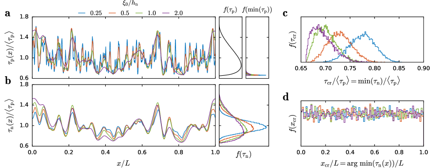
Figure 5: Analytical Monte Carlo study. (a) The random local friction strength $\tau_{\mathrm{p}}(x)$ is generated with different correlation lengths $\xi_{0}$. For visual purposes, the same random seed is used for the 4 cases shown. (b) The corresponding local nucleation strength $\tau_{\mathrm{n}}(x)$ is computed using (Eq. 9). The probability densities $f$ of the random fields $\tau_{\mathrm{n}}$, $\min(\tau_{\mathrm{n}})$ and $\tau_{\mathrm{p}}$ are reported on the right of (a) and (b), respectively and computed using $N=10,000$ samples. $f(\min(\tau_{\mathrm{p}}))$ and $f(\tau_{\mathrm{n}})$ depend on $\xi_{0}$. (c) Probability density of the global friction strength $\tau_{\mathrm{cr}}$. (d) Probability density of the position of the critical nucleation patch $x_{\mathrm{cr}}$. Note that the seed is not fixed anymore for the samples used in (c) and (d).

Prior to presenting the numerical results we provide some intuition of the effect of correlation length on the nucleation strength $\tau_{\mathrm{n}}$ based on probabilistic arguments. By exploiting the stationarity of $\tau_{\mathrm{p}}$ and $\tau_{\mathrm{n}}$ it is possible to derive an analytical expression of the expectation of the nucleation strength $\mathrm{E}[\tau_{\mathrm{n}}]$ and its variance $\mathrm{Var}[\tau_{\mathrm{n}}]$ as function of the corresponding statistical properties of local strength, $\mathrm{E}[\tau_{\mathrm{p}}]$, $\mathrm{Var}[\tau_{\mathrm{p}}]$ and $\xi_{0}/h_{\mathrm{n}}$ (see B).

One interesting finding is that the expectation is not affected by $\xi_{0}/h_{\mathrm{n}}$: $\mathrm{E}[\tau_{\mathrm{n}}]=\mathrm{E}[\tau_{\mathrm{p}}]$ (see derivation in Eq. 23). The expression for $\mathrm{Var}[\tau_{\mathrm{n}}]$, however, involves a double integral of the product of the correlation function $C(.)$ and the eigenfunction $v_{0}(.)$, which can be evaluated numerically (see derivation in Eq. 24). For perfect correlation, i.e., $\xi_{0}/h_{\mathrm{n}}=\infty$, $C(.)$ becomes a constant, thus $\mathrm{Var}[\tau_{\mathrm{n}}]=\mathrm{Var}[\tau_{\mathrm{p}}]$. Additionally, in the limit of $\xi_{0}\ll h_{\mathrm{n}}$, the double integral in Eq. 24 scales with $\xi_{0}/h_{\mathrm{n}}$, thus $\mathrm{Var}[\tau_{\mathrm{n}}]\propto\mathrm{Var}[\tau_{\mathrm{p}}]{\xi_{0}}/{h_{\mathrm{n}}}$ (see derivation in Eq. 26).

We consider a range of correlation lengths $\xi_{0}/h_{\mathrm{n}}=\{0.25,0.5,1.0,2.0\}$, while all other properties remain constant. Fig. 5a-left shows one sample of $\tau_{\mathrm{p}}(x)$ for each considered $\xi_{0}$. For clarity of visualization, in Fig. 5a we use the same seed when generating the random fields. Hence, the fields have the same modal random amplitudes $A_{j}$ and $B_{j}$, see Eq. 5, but have different modal spectral densities $\sigma_{j}^{2}$, corresponding to the different $\xi_{0}$. For this reason, all shown samples have a similar spatial evolution and the effect of varying $\xi_{0}$ can be clearly observed. By definition, all $\tau_{\mathrm{p}}(x)$ samples are drawn from the same probability distribution $f(\tau_{\mathrm{p}})$ (see Fig. 5a-center). Decreasing $\xi_{0}$, moves the probability density of its minimum $f(\min(\tau_{\mathrm{p}}))$ towards the lower bound $\tau_{\mathrm{p}}^{\mathrm{min}}=0.66\langle\tau_{\mathrm{p}}\rangle$ (see Fig. 5a-right), because with lower correlation lengths it is more likely to visit a broad range of $\tau_{\mathrm{p}}$ values.

Fig. 5b-left shows the corresponding nucleation strength $\tau_{\mathrm{n}}(x)$ for each of the local frictional strength fields $\tau_{\mathrm{p}}(x)$ presented in Fig. 5a, computed using Eq. 13. As mentioned before, $\tau_{\mathrm{n}}$ is essentially a weighted moving average of $\tau_{\mathrm{p}}$ with window size $h_{\mathrm{n}}$ (see Eq. 9). Thus, most of the high frequency content of $\tau_{\mathrm{p}}$ disappears and the effect of $\xi_{0}$ on $\tau_{\mathrm{n}}$ is more subtle. One interesting feature is in the minima and maxima of $\tau_{\mathrm{n}}$: increasing $\xi_{0}$ causes lower minima and higher maxima, because the moving average is effectively computed over an approximately constant field $\tau_{\mathrm{n}}\approx\tau_{\mathrm{p}}$. Inversely, decreasing $\xi_{0}$ causes the opposite effect and $\tau_{\mathrm{n}}\approx\langle\tau_{\mathrm{p}}\rangle$.

This effect is more clearly visible by considering the distribution $f(\tau_{\mathrm{n}})$ shown in Fig. 5b-right. Increasing $\xi_{0}$ effectively puts more weight onto the tails of $f(\tau_{\mathrm{n}})$ (see $\xi_{0}/h_{\mathrm{n}}=2.0$ in Fig. 5b-right), and in the limiting case of $\xi_{0}/h_{\mathrm{n}}\rightarrow\infty$ the distribution of $\tau_{\mathrm{n}}$ will be the same as the one of $\tau_{\mathrm{p}}$ (analogous to Eq. 25). On the other hand, decreasing $\xi_{0}$ puts weight on its mean $\langle\tau_{\mathrm{p}}\rangle$, making $f(\tau_{\mathrm{n}})$ similar to a Gaussian (see $\xi_{0}/h_{\mathrm{n}}=0.25$ in Fig. 5b-right) with variance proportional to $\xi_{0}$ (see Eq. 26). In the limit $\xi_{0}/h_{\mathrm{n}}\rightarrow 0$ the distribution of $\tau_{\mathrm{n}}$ becomes a Dirac-$\delta$ centered at $\langle\tau_{\mathrm{p}}\rangle$. The described dependence of $f(\tau_{\mathrm{n}})$ on $\xi_{0}$ confirms the previously stated statistical arguments (see B for derivation).

Because $f(\tau_{\mathrm{p}})$ is skewed towards the lower bound of $\tau_{\mathrm{p}}$ so is $f(\tau_{\mathrm{n}})$; the larger $\xi_{0}$ the larger the skewness. For $\tau_{\mathrm{cr}}$ this effect is amplified by the fact that $\tau_{\mathrm{cr}}=\min(\tau_{\mathrm{n}}(x))$ as depicted in Fig. 5c, causing $\langle\tau_{\mathrm{cr}}\rangle$ to decrease with increasing $\xi_{0}$. As noted in Sec. 3.3, the location where the critical instability occurs $x_{\mathrm{cr}}$ is uniformly distributed over the entire domain as shown in Fig. 5d and is independent on $\xi_{0}$.

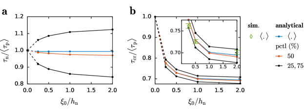
Figure 6: Variation of nucleation strength $\tau_{\mathrm{n}}$ (a) and effective friction strength $\tau_{\mathrm{cr}}$ (b) as function of correlation length $\xi_{0}$. Solid lines are the results from the analytical Monte Carlo study with $N=10,000$ (same data as Fig. 5). Data-points for $\xi_{0}/h_{\mathrm{n}}\rightarrow 0$ are based on analytical considerations and connected to the analytical Monte Carlo results by dashed lines. Diamonds are results from 60 dynamic simulations (same data as Fig. 4).

We further analyze the effect of $\xi_{0}$ on the probability distribution of $\tau_{\mathrm{n}}$ and $\tau_{\mathrm{cr}}$ by reporting the mean, median and $25\%$ percentile of the probability density function (see Fig. 6). We observe that the nucleation strength tends towards the mean peak strength for vanishing correlation length, $\lim_{\xi_{0}/h_{\mathrm{n}}\rightarrow 0}\tau_{\mathrm{n}}(x)=\langle\tau_{\mathrm{p}}\rangle$, because the moving average in computing $\tau_{\mathrm{n}}(x)$ is evaluated over a window $h_{\mathrm{n}}$ that appears infinite compared to $\xi_{0}$ (see Fig. 6a). Consequently, the effective strength also tends towards the mean of the local strength: $\lim_{\xi_{0}/h_{\mathrm{n}}\rightarrow 0}\tau_{\mathrm{cr}}=\langle\tau_{\mathrm{p}}\rangle$ (see Fig. 6b). Conversely, if ${\xi_{0}\gg h_{\mathrm{n}}}$, the moving average is computed over a window $h_{\mathrm{n}}$ which vanishes, and thus (9) becomes the identity: $\lim_{\xi_{0}/h_{\mathrm{n}}\rightarrow\infty}\tau_{\mathrm{n}}(x)=\tau_{\mathrm{p}}(x)$. In this case, the effective strength will be more likely to be close to the actual lower bound of the distribution $\lim_{\xi_{0}/h_{\mathrm{n}}\rightarrow\infty}\tau_{\mathrm{cr}}=\min(\tau_{\mathrm{p}})$ (see Fig. 6b). The transition between these two limiting cases is described by the results of the analytical Monte Carlo study, which are validated by 20 dynamic simulations for each $\xi_{0}/h_{\mathrm{n}}$ by reporting the mean effective friction strength (see inset in Fig. 6b). For $\xi_{0}/h_{\mathrm{n}}\geq 0.5$ simulations and theory coincide. However, for $\xi_{0}/h_{\mathrm{n}}=0.25$ the theoretical model slightly overestimates the effective friction strength. In Sec. 5, we will argue that the lower effective friction at small $\xi_{0}/h_{\mathrm{n}}$ is caused by interactions between neighbouring nucleation patches, which destabilize each other and lead to unstable growth at lower overall loading compared to the theoretical prediction.

5 Discussion

5.1 Implications of the Physical Problem

The analyzed physical problem is simplistic and contains only the absolute minimum of a realistic system with a frictional interface – while still maintaining a rigorous representation of the constitutive relation of the bulk and the interface. The objective is to provide a fundamental understanding of the macroscopic effects on static friction caused by randomness in the local frictional properties. While many options exist to complexify the proposed system, we leave them for future work and focus here on the basics. Nevertheless, in this section, we will discuss some of these simplifications as well as their implications.

Randomness along the interface may have various origins including heterogeneity in bulk material properties and local environmental conditions (e.g., humidity and impurities). Prominent causes for randomness are geometric imperfections, which include non-flat interfaces and surface roughness. The real contact area, which is an ensemble of discrete micro-contacts (Bowden and Tabor, 1950; Dieterich and Kilgore, 1994; Li and Kim, 2008; Sahli et al., 2018) and is much smaller than the apparent contact area, introduces naturally randomness to the interface. Surface roughness is often modeled as self-affine fractals (Pei et al., 2005), which directly affects the size distribution of micro-contacts and local contact pressure. The resulting frictional properties are expected to vary similarly. This would typically lead to small areas of the interface with high frictional strength and most areas with no resistance against sliding, i.e., $\tau_{\mathrm{p}}=0$, since only the micro-contacts may transmit stresses across the interface. Therefore, at this length scale, one would expect the random strength field to be bound by zero at most locations, similar to the approach taken by Barras et al. (2019). However, in many engineering systems, the nucleation length is orders of magnitude larger than the characteristic length scales of the micro-contacts: nucleation lengths of $\sim 10-100~{}\mathrm{mm}$ (Ben-David and Fineberg, 2011; Latour et al., 2013) and surface roughness lengths of $\sim 1~{}\mu\mathrm{m}$ (Svetlizky and Fineberg, 2014). For this reason, we consider a continuum description with a somewhat larger length scale. In our approach, the frictional strength profile is continuous and varies due to randomness in the micro-contacts population without considering individual contact points.

Surface roughness and other local properties directly affect how frictional strength changes depending on slip $\delta$, slip rate $\partial_{t}\delta$, and state (Rabinowicz, 1995; Pilvelait et al., 2020). This is often modeled in phenomenological rate-and-state friction models (Dieterich, 1979; Ruina, 1983; Rice and Ruina, 1983). As discussed by Garagash and Germanovich (2012) and demonstrated by Rubin and Ampuero (2005) and Ampuero and Rubin (2008), the nucleation length scale of rate-and-state friction models approaches asymptotically the critical length $h_{\mathrm{n}}$ used in this work and given by Eq. 8 if the rate-and-state friction parameters are favoring strong weakening with slip rate. However, if rate-weakening becomes negligible, the nucleation criterion tends towards the Griffith’s length (Andrews, 1976), which applies to ruptures with small-scale yielding. In this case, the frictional weakening process is contained in a small zone at the rupture tip and most of the rupture surface is at the residual stress level, which is different to the nucleation patches by Uenishi and Rice (2003), where the entire rupture surface is still weakening when the critical length is reached.

Since many engineering materials present relatively important slip-rate weakening friction, e.g., dynamic weakening of $\sim 1~{}\mathrm{MPa}$ for glassy polymers at normal pressure of $\sim 5~{}\mathrm{MPa}$ (Svetlizky et al., 2020) and, similarly, $\sim 1~{}\mathrm{MPa}$ weakening for granite at normal pressure of $\sim 6~{}\mathrm{MPa}$ (Kammer and McLaskey, 2019), we considered a model system with strong frictional weakening. However, we neglect the complexity of rate-and-state friction, as extensively demonstrated by Ray and Viesca (2017, 2019), and apply a linear slip-weakening friction law at the interface because it has the most important features of friction, i.e., a weakening mechanism, while being simple and well-understood. The advantage is that the weakening-rate $W$ is predefined. It further has a well-defined fracture energy $\Gamma$, which is the energy dissipated by the weakening process, i.e., the triangular area $(\tau_{\mathrm{p}}-\tau_{\mathrm{r}})d_{\mathrm{c}}/2$ in Fig. 1c:

$$\Gamma(x)=\frac{(\tau_{\mathrm{p}}(x)-\tau_{\mathrm{r}})^{2}}{2W}~{}.$$ (14)

Since $W$ is constant in our system $\Gamma$ varies with $(\tau_{\mathrm{p}}(x)-\tau_{\mathrm{r}})^{2}$. A correlation between $\Gamma(x)$ and $\tau_{\mathrm{p}}(x)$ can be expected given that any point that is stronger, i.e., increased $\tau_{\mathrm{p}}$, is likely to dissipate more energy as well, i.e., increased $\Gamma$.

Further, the linear slip-weakening law is contact-pressure independent, which may appear counter-intuitive based on Coulomb’s well-known friction laws (Amontons, 1699; Coulomb, 1785). However, the contact pressure is, due to symmetry in similar-material interfaces, constant over time and, therefore, any possible pressure dependence becomes irrelevant for the nucleation process itself. Nevertheless, local friction properties are expected to change for systems with different normal pressure. This effect has not been analyzed here since we did not vary the contact pressure, but could be taken into account by changing the values of $\tau_{\mathrm{p}}$, $\tau_{\mathrm{r}}$ and $d_{\mathrm{c}}$.

Finally, we note that by assuming a periodic system, we neglect possible boundary effects. We expect that the boundary would locally reduce $\tau_{\mathrm{cr}}$ compared to the prediction based on Eq. 10, which assumes an infinite domain, because the free boundary would locally restrict stress redistribution and thus increase the stress at the edge of the nucleation patch. Therefore, the probability density of global frictional strength $\tau_{\mathrm{cr}}$ for a periodic system, as shown in Fig. 5c, has likely a slight tendency towards higher values compared to a finite system. However, we expect the spatial range of the boundary effect to scale with $h_{\mathrm{n}}$ and, therefore, $f(\tau_{\mathrm{cr}})$ will tend towards the periodic solution for $h_{\mathrm{n}}/L\rightarrow 0$. Verification would require a large number of numerical simulations, which is beyond the scope of this work.

5.2 Interpretation of Numerical Simulations

The simulations have shown that uniform $\tau_{0}$ and random $\tau_{\mathrm{p}}(x)$ cause multiple nucleation patches to develop simultaneously. We can see in Fig. 3b-right that $20$-$30$ patches (bright blue stripes) coexist by the time global strength is reached, i.e., $t/T=1$. Most of these nucleation patches grow very slowly and their number increases with increasing $\tau_{0}(t)$. Nucleation patches can also merge, which is what happens in this simulation to the critical patch. Furthermore, the simulation shows that unstable growth and thus global failure is not necessarily caused by the first nucleation patch to appear. For instance, the $\tau_{\mathrm{p}}(x)$ profile shown in Fig. 3c presents three local minima with approximately the same value, i.e., at $x/L\approx 0.4$, $0.6$ and $0.75$. Therefore, the first three nucleation patches appear quasi-simultaneously. Whether one of these patches or another one appearing later is the one becoming unstable first does only dependent indirectly on the minimum value of $\tau_{\mathrm{p}}(x)$. More important is whether $\tau_{\mathrm{p}}(x)$ remains low in the near region of the local minimum. The nucleation patch at $x/L\approx 0.75$ is in an area of relatively low $\tau_{\mathrm{p}}(x)$, compared to the other early nucleation patches, which is why it develops faster to the critical size and causes unstable propagation.

This non-local character of the nucleation patches becomes obvious when considering the integral form of Eq. 9 that corresponds to a weighted moving average of $\tau_{\mathrm{p}}(x)$. In Fig. 4a, we can see that $\tau_{\mathrm{n}}$ at $x/L\approx 0.75$ is considerably lower than at the location of the other early nucleation patches $x/L\approx 0.4$ and 0.6. This is why $x/L\approx 0.75$ gets critical first and causes unstable slip area growth. Interestingly, $x/L\approx 0.3$ is the second most critical point even though the local minimum in $\tau_{\mathrm{p}}$ is higher than many others in this system. However, $\tau_{\mathrm{p}}(x)$ remains rather low over an area that approaches $h_{\mathrm{n}}$, and therefore $\tau_{\mathrm{n}}$ is also low.

In Fig. 4, we compared the prediction of $\tau_{\mathrm{cr}}$ with measurements from simulations and showed that the prediction works generally well. However, we noticed that for decreasing $\xi_{0}/h_{\mathrm{n}}$ the discrepancies increase. The theory generally predicts higher $\tau_{\mathrm{cr}}$ than observed in simulations. We believe that this is caused by nucleation patch interaction, which is neglected in the current theory. The interaction may occur if two nucleation patches are near each other. Nucleation patches cause stress redistribution because the stress inside the patch decreases but, due to equilibrium, it increases in the area near the patch. Therefore, a nucleation patch may cause an increase of the effective stress (compared to the applied load) to another patch, which leads to increased patch size and thus $h_{\mathrm{n}}$ is reached already at $\tau_{\mathrm{cr}}^{\mathrm{sim}}<\tau_{\mathrm{cr}}^{\mathrm{pred}}$. Interestingly, a similar phenomenon has recently been observed in simulations of compressive failure governed by a mesoscopic Mohr-Coulomb criterion, where local damage clusters interact and eventually coalesce to macroscopic failure (Dansereau et al., 2019).

The nucleation patch interaction is likely also the cause for discrepancies observed in the prediction of the nucleation location $x_{\mathrm{cr}}$, as shown in Fig. 4c. While most cases are very well predicted, some simulations present unstable growth that starts from a different location. In these cases, two nucleation patches have very similar critical stress level. However, the (slightly) less critical patch interacts with a neighboring smaller patch and thus becomes unstable at a lower stress level than theoretically expected. This is more likely to occur for systems with low $\xi_{0}/h_{\mathrm{n}}$ since this increases the likelihood of another local minimum being located close to active nucleation patches. Nevertheless, the critical stress level $\tau_{\mathrm{cr}}$ remains quantitatively well predicted, as shown Fig. 4b and discussed above, because these secondary effects are minor.

The representative simulation illustrated in Fig. 3 shows that the frictional rupture front, after becoming unstable, does not arrest until it propagated across the entire interface leading to global sliding. This is a general feature of our problem and all our simulations present the same behavior. What is the reason for this run-away propagation? Right after nucleation, the slipping area continues to weaken along its entire length, i.e., $\delta<d_{\mathrm{c}}$ everywhere. However, after some more growth, it transforms slowly into a frictional rupture front, which is essentially a Griffith’s shear crack with a cohesive zone and constant residual strength (Svetlizky and Fineberg, 2014; Svetlizky et al., 2020; Garagash and Germanovich, 2012). The arrest of frictional rupture fronts are governed by an energy-rate balance (Kammer et al., 2015), which states that a rupture continues to propagate as long as the (mode II) static energy release rate $G_{\mathrm{II}}$ is larger than the fracture energy, i.e., $G_{\mathrm{II}}>\Gamma$. In our system, the stress drop $\Delta\tau=\tau_{0}-\tau_{\mathrm{r}}$ is uniform since $\tau_{0}$ and $\tau_{\mathrm{r}}$ are uniform. Thus, the static energy release rate grows linearly with rupture length $G_{\mathrm{II}}\propto h$, and it becomes increasingly difficult to arrest a rupture as it continues to grow. Specifically for our case, we find that $G_{\mathrm{II}}>\Gamma_{\mathrm{max}}$ for $h/h_{\mathrm{n}}\gtrapprox 3$, where $\Gamma_{\mathrm{max}}$ is $\Gamma$ from Eq. 14 for $\tau_{\mathrm{p}}^{\mathrm{max}}$. Hence, once the slipping area reached a size of $h/h_{\mathrm{n}}\gtrapprox 3$, nothing can stop it anymore – not even $\tau_{\mathrm{p}}^{\mathrm{max}}$. For $h/h_{\mathrm{n}}\lessapprox 3$, it is theoretically possible for the slipping area to arrest after some unstable propagation. However, a large increase in $\tau_{\mathrm{p}}(x)$ would need to occur simultaneously on both side, which is very unlikely, in particular for $\xi_{0}/h_{\mathrm{n}}>1$. Therefore, our assumptions of constant stress drop $\Delta\tau$ and limited variation of local frictional strength causes arrested rupture fronts to be extremely rare. Nevertheless, since $\Gamma_{\mathrm{max}}$ depends on the probability distribution function $f(\tau_{\mathrm{p}})$, a larger variance, and thus a larger $\tau_{\mathrm{p}}^{\mathrm{max}}$, would make crack arrest (slightly) more likely.

It is interesting to note, however, that arrest of dynamically propagating slipping areas may occur in other systems. Amon et al. (2017), for instance, showed in their simulations that multiple smaller events nucleate and arrest in order to prepare the interface for a global event. In their system, the initial position along the interface is random as well as the friction properties. Therefore, the available elastic energy, which is the driving force, is random and may fluctuate enough to cause arrest. For the same reason, Geus et al. (2019) observed arrested events of various sizes in simulations with random potential energy along the interface. On the contrary, our system, as outlined above, is characterized by steadily increasing available energy and, thus, behaves differently.

Experimental evidence for arrest of frictional rupture fronts is rather limited. The arrest of confined events observed by Rubinstein et al. (2007) on glassy polymers and by Ke et al. (2018) on granite, is caused by non-uniform loading due to the experimental configuration as demonstrated by Kammer et al. (2015) and Ke et al. (2018, 2019). While small scale randomness in the applied shear stress may occur, it does not cause arrest – at best, it may slightly delay or expedite it. Therefore, these experimental observations do not support the presence of any important randomness in the applied shear load; at least at these scales. In much larger systems, such as tectonic plates, randomness in the background stress is likely very important, as discussed in Sec. 5.4.

5.3 Interpretation of Monte Carlo Study

In an engineering context, it is usually not enough to know the mean value of a macroscopic property, e.g., the static friction strength, since design criteria are determined based on probability of failure; and risk assessments require failure probability analysis. If the stochastic properties of local interfacial strength $\tau_{\mathrm{p}}(x)$ are known, the developed theoretical framework in Sec. 4 provides a tool to evaluate the global strength distribution and, hence, the failure probability. However, $\tau_{\mathrm{p}}(x)$ is not directly observable in experiments (at least so far). In the absence of experimental evidence, the stochastic properties of $\tau_{\mathrm{p}}(x)$ have been chosen based on physical considerations but our specific parameter choice is arbitrary. This approach is a first approximation that enables us to develop an efficient Monte Carlo method to study the effects of such variations on macroscopic properties. This method may be adapted to more realistic random friction profiles. In the following section we will discuss the choice of each stochastic property of $\tau_{\mathrm{p}}(x)$ and its effect on the variability of global strength, $\tau_{\mathrm{cr}}$.

We assumed that $\tau_{\mathrm{p}}(x)$ is a random variable following a Beta distribution because it provides simultaneously a non-Gaussian property and well-defined boundaries for minimum and maximum strength, which is physically consistent since mechanical properties are bounded. The parameters of the Beta distribution are chosen such that it is skewed towards the lower bound of $\tau_{\mathrm{p}}$. Physically this means that the local interface strength is mostly weak with few strong regions. Under this assumption we observed that the global interface strength $\tau_{\mathrm{cr}}$ is close the lower bound of $\tau_{\mathrm{p}}$ and that decreasing correlation length $\xi_{0}$ leads to higher $\tau_{\mathrm{cr}}$ with smaller variation (see Fig. 6). Nucleation is governed by the strength of the weakest region which size equals or exceeds the nucleation length. Hence, if the skewness would be toward high values of $\tau_{\mathrm{p}}$ – this would corresponds to a mostly strong interface with few weak regions – the variation of $\tau_{\mathrm{cr}}$ would be larger because of the longer tail at the lower bound. However, the effect of correlation length would remain unchanged: lower $\xi_{0}$ would cause higher $\tau_{\mathrm{cr}}$ with smaller variation.

Further, we assumed that $\tau_{\mathrm{p}}$ has a power spectral density specified in Eq. 4 with a specific exponent, which affects the memory of the random field. A smaller exponent would result in a flatter decay above the cutoff frequency, and thus generate a field with more high-frequency content. However, when considering equivalent correlation lengths, effects of different assumptions regarding the functional form of the power spectral density are expected to be minor in the probability density of $\tau_{\mathrm{cr}}$.

It is noteworthy that there are three relevant length scales: $L$, $h_{\mathrm{n}}$ and $\xi_{0}$. Here, we have not considered the effects of changes in $L$ so far. Based on our theoretical model, we expect that a larger $L$ would result in smaller variance of $\tau_{\mathrm{cr}}$. One approach to explore this effect, while avoiding to change the size of the experimental system, could be to modify the normal load, which would affect $\tau_{\mathrm{p}}$ and $\tau_{\mathrm{r}}$, and hence the critical nucleation size $h_{\mathrm{n}}\propto(\tau_{\mathrm{p}}-\tau_{\mathrm{r}})^{-1}$, as shown experimentally by Latour et al. (2013).

5.4 Implications for Earthquake Nucleation

In the current study, we are interested in estimating the probability distribution of the macroscopic strength of a frictional interface of given size $L$. Similar systems but with a focus on other aspects have been studied in order to gain a better understanding of earthquake nucleation. The challenges in studying earthquake nucleation are associated with the size of the system (hundreds of kilometers) and the limited physical access to measure important properties, such as stress state and frictional properties. However, when and how an earthquake nucleates affects directly the average stress drop level $\langle\Delta\tau\rangle\equiv\tau_{\mathrm{cr}}-\tau_{\mathrm{kin}}$, and the earthquake magnitude, which is more easily determined. Hence, there is a need to infer from earthquake magnitude observation back on the fault properties and their variability, to learn about the risk of potential future earthquakes. This is a similar inverse problem as described above.

Previous studies have shown that randomness in simplified models present earthquake magnitudes that follow a power-law distribution (Carlson and Langer, 1989; Ampuero et al., 2006). The simulations presented a large range of magnitudes because the slipping areas arrested, which is the result of randomness in the local stress drop, as discussed in Sec. 5.2. Interestingly, small events were shown to smoothen the stress profile, which reduces the randomness, thus prepared the interface for larger events, as also observed experimentally (Ke et al., 2018). This would suggest that nucleation of larger events tend to be caused by randomness in fault properties rather than (background) stress level, since the stress is getting smoothed. Therefore, our model provides a simple but reasonable tool to study nucleation of medium to large earthquakes.

Our results show that smaller correlation length lead to higher overall strength and more variation. In the context of earthquakes, this would suggest that smaller $\xi_{0}/h_{\mathrm{n}}$ support larger earthquake magnitudes since nucleation at a higher stress level translates into larger average stress drops, which provides more available energy to release and, thus, makes arrest more difficult. This is complementary to observations by Ampuero et al. (2006) that showed a trend to higher earthquake magnitudes for decreasing standard deviation of the random stress drop field $\Delta\tau(x)$ while keeping $\xi_{0}/h_{\mathrm{n}}$ constant.

In addition to the important question on critical stress level for earthquake nucleation, it also remains unclear how the nucleation process takes place. Two possible models (Beroza and Ellsworth, 1996; Noda et al., 2013; McLaskey, 2019) are discussed. The ”Cascade” model, where foreshocks trigger each other with increasing size and finally lead to the main earthquake; and the ”Pre-Slip” model, which assumes that nucleation is the result of aseismic slow-slip. In our simplistic model, nucleation occurs in a ”Pre-Slip” type process, with a long phase of slow slip and an abrupt acceleration after the nucleation patch reached its critical size (see Fig. 3b-right). However, if the amplitude range of our random $\tau_{\mathrm{p}}(x)$ field was much larger, the likelihood of arrest would increase and, thus, interaction between arrested small events could emerge. This would lead to a nucleation process that resembles more the ”Cascade” model. We, therefore, conclude that the type of nucleation process that may occur at a given fault depends on extent of randomness in the local stress and property fields.

6 Conclusion

We studied the stochastic properties of frictional interfaces considering the nucleation of unstable slip patches. We considered a uniform loading condition and studied the effect of random interface strength, characterized by its probability density and correlation function. Using numerical simulations solving the elastodynamic equations, we demonstrated that macroscopic sliding does not necessarily occur when the weakest point along the interface starts sliding, but when one of possible many slowly slipping nucleation patches reaches a critical length and becomes unstable. We verified that the nucleation criterion originally developed by Uenishi and Rice (2003) predicts well the critical stress leading to global sliding if the criterion is formulated as a minimum of the local strength convolved with the first eigenfunction of the elastic problem. The simulations further showed that increasing correlation lengths of the random interface strength lead to reduced macroscopic static friction. Using the theoretical nucleation criterion, we perform a Monte Carlo study that provided an accurate description of the underlying probability density functions for these observed variations in macroscopic friction. We showed that the probability density function of the global critical strength approaches the probability density of the minimum in the random local strength when the correlation length is much larger than the critical nucleation length. Conversely, a vanishingly small correlation length results in generally higher macroscopic strength with smaller variation. We showed that the presence of precursory dynamic slip events, as in more complex models, is extremely unlikely under the assumption of uniform stress drop. Finally, we discussed discrepancies between the theoretical model and simulations, which suggest that for small correlation lengths the theoretical prediction overestimates the frictional strength, possibly because it neglects interactions between neighboring nucleation patches.

Appendix A Nucleation Criterion

The nucleation criterion used in this work is based on the theory developed by Uenishi and Rice (2003). It is not our intention of re-deriving the theoretical framework. Nevertheless, in this section, we provide a clear problem statement such that our work can easily be related to the work by Uenishi and Rice (2003). The peak strength along the interface is given by

$$\tau_{\mathrm{p}}(x)=\tau_{\mathrm{p}}^{\mathrm{min}}+q(x)~{},$$ (15)

where $\tau_{\mathrm{p}}^{\mathrm{min}}$ is the minimum value of $\tau_{\mathrm{p}}(x)$. The functional form $q(x)$ satisfies $q(x_{m})=0$ and $q(x)>0$ for $x\neq x_{m}$. If local slip occurs at any point along the interface, the local strength decreases because of the slip-weakening friction law, as defined by Eq. 1. Therefore, any point that is in the weakening process, i.e., $d_{\mathrm{c}}>\delta(x,t)>0$, presents a local shear stress that is given by

$$\tau(x)=\tau_{\mathrm{p}}(x)-W\delta(x,t)=\tau_{\mathrm{p}}^{\mathrm{min}}+q(x)-W\delta(x,t)~{},$$ (16)

where Eq. 15 was used and the weakening rate satisfies $W>0$.

The applied shear stress, which starts at the level of the minimum strength, is defined by

$$\tau_{0}(t)=\tau_{\mathrm{p}}^{\mathrm{min}}+Rt~{},$$ (17)

where $R>0$ is the shear-stress loading rate.

Following Uenishi and Rice (2003), we can consider the quasi-static elastic equilibrium (Bilby and Eshelby, 1968) that relates the stress change along the interface with the local slip through

$$\tau(x,t)=\tau_{0}(x,t)-\frac{G^{*}}{2\pi}\int_{a_{-}(t)}^{a_{+}(t)}\frac{\partial\delta(\xi,t)/\partial\xi}{x-\xi}\mathrm{d}\xi~{},$$ (18)

where $G^{*}=G/(1-\nu)$ and $a_{-}(t)<x<a_{+}(t)$ are the boundaries of the slowly expanding slipping area. By substituting Eq. 16 and Eq. 17 into Eq. 18, we find

$$-W\delta(x,t)=Rt-q(x)-\frac{G^{*}}{2\pi}\int_{a_{-}(t)}^{a_{+}(t)}\frac{\partial\delta(\xi,t)/\partial\xi}{x-\xi}\mathrm{d}\xi~{},$$ (19)

for $\delta(x,t)>0$ and $a_{-}(t)<x<a_{+}(t)$. This corresponds exactly to (Uenishi and Rice, 2003, Eq.4).

Starting from this equation, Uenishi and Rice (2003) show that quasi-static solutions cease to exist for slipping areas larger than a critical length $h_{\mathrm{n}}$, which is given by

$$h_{\mathrm{n}}\approx 1.158\frac{G^{*}}{W}~{}.$$ (20)

Interestingly, the critical length only depends on the shear modulus $G^{*}$ and the slip-weakening rate $W$, and is independent of the loading rate $R$ and the shape of the peak strength $q(x)$.

Uenishi and Rice (2003) further show that a slipping area exceeding $h_{\mathrm{n}}$ is reached at time $t_{c}$ when the critical stress level is given by (Uenishi and Rice, 2003, Eq.14)

$$Rt_{c}\approx 0.751\int_{-1}^{+1}q[a(t_{c})s+b(t_{c})]v_{0}(s)\mathrm{d}s~{},$$ (21)

where $a(t)=[a_{+}(t)-a_{-}(t)]/2$ and $b(t)=[a_{+}(t)+a_{-}(t)]/2$ are the half-length and center location of the slipping area, respectively, and $s=[x-b(t)]/a(t)$ and $v_{0}(s)\approx(0.925-0.308s^{2})\sqrt{1-s^{2}}$. It becomes obvious that the stress level at which the slipping area reaches the critical length depends on the shape of $q(x)$.

Appendix B Simplified Statistical Analysis of the Nucleation Strength

In order to give some intuition of the effects of correlation length $\xi_{0}$ on the nucleation strength $\tau_{\mathrm{n}}$ (Eq. 9), we provide a statistical argument, which is based on the property of stationarity of $\tau_{\mathrm{p}}$. Note that $v_{0}(.)$ has the following property

$$0.751\int_{-1}^{+1}v_{0}(s)\mathrm{d}s=1$$ (22)

We aim to evaluate the expectation and variance of $\tau_{\mathrm{n}}$ as function of $\xi_{0}$. The expectation is an integral with respect to a probability measure rather than a Lebesgue measure. Since $\tau_{\mathrm{p}}$ and $\tau_{\mathrm{n}}$ are stationary, we can apply the Fubini’s theorem, which states that the order of integration can be changed, and express the expectation $\mathrm{E}[\tau_{\mathrm{n}}]$ as function of the expectation of the local strength $\mathrm{E}[\tau_{\mathrm{p}}]$.

$$\begin{split}\mathrm{E}[\tau_{\mathrm{n}}]&=\mathrm{E}\left[0.751\int_{-1}^{+1}\tau_{\mathrm{p}}\left(s\,h_{\mathrm{n}}/2+x\right)v_{0}(s)\mathrm{d}s\right]=0.751\int_{-1}^{+1}\mathrm{E}\left[\tau_{\mathrm{p}}\left(s\,h_{\mathrm{n}}/2+x\right)\right]v_{0}(s)\mathrm{d}s\\ &=\mathrm{E}[\tau_{\mathrm{p}}]0.751\int_{-1}^{+1}v_{0}(s)\mathrm{d}s=\mathrm{E}[\tau_{\mathrm{p}}]\end{split}$$ (23)

Similarly, we can express its variance $\mathrm{Var}[\tau_{\mathrm{n}}]$ as function of the variance of the local strength $\mathrm{Var}[\tau_{\mathrm{p}}]$ by applying Fubini’s Theorem and the definition of the correlation function $C(\xi)=\mathrm{E}[(\tau_{\mathrm{p}}(x)-\mathrm{E}[\tau_{\mathrm{p}}])(\tau_{\mathrm{p}}(x+\xi)-\mathrm{E}[\tau_{\mathrm{p}}])/\mathrm{Var}[\tau_{\mathrm{p}}]$

$$\begin{split}\mathrm{Var}[\tau_{\mathrm{n}}]&=\mathrm{E}[(\tau_{\mathrm{n}}(x)-\mathrm{E}[\tau_{\mathrm{n}}])^{2}]=\mathrm{E}\left[\left(0.751\int_{-1}^{+1}\tau_{\mathrm{p}}\left(s\,h_{\mathrm{n}}/2+x\right)v_{0}(s)\mathrm{d}s-\mathrm{E}[\tau_{\mathrm{p}}]\right)^{2}\right]\\ &=\mathrm{E}\left[\left(0.751\int_{-1}^{+1}\left(\tau_{\mathrm{p}}\left(s\,h_{\mathrm{n}}/2+x\right)-\mathrm{E}[\tau_{\mathrm{p}}]\right)v_{0}(s)\mathrm{d}s\right)^{2}\right]\\ &=0.751^{2}\iint_{[-1,1]^{2}}\mathrm{E}\left[\left(\tau_{\mathrm{p}}\left(s\,h_{\mathrm{n}}/2+x\right)-\mathrm{E}[\tau_{\mathrm{p}}]\right)\left(\tau_{\mathrm{p}}\left(t\,h_{\mathrm{n}}/2+x\right)-\mathrm{E}[\tau_{\mathrm{p}}]\right)\right]v_{0}(s)v_{0}(t)\mathrm{d}s\,\mathrm{d}t\\ &=\mathrm{Var}[\tau_{\mathrm{p}}]0.751^{2}\iint_{[-1,1]^{2}}C((s-t)h_{\mathrm{n}}/2)v_{0}(s)v_{0}(t)\mathrm{d}s\,\mathrm{d}t\end{split}$$ (24)

For the limiting cases the expression for the variance can be expressed analytically. For perfectly correlated $\tau_{\mathrm{p}}$, $\xi_{0}=\infty$, $C(.)=1$

$$\lim_{\xi_{0}/h_{\mathrm{n}}\rightarrow\infty}\mathrm{Var}[\tau_{\mathrm{n}}]=\mathrm{Var}[\tau_{\mathrm{p}}]$$ (25)

Both $C(.)$ and $v_{0}(.)$ are known. Therefore, the integral of Eq. 24 can be solved numerically (see Fig.7). For $\xi_{0}\ll h_{\mathrm{n}}$ the correlation function $C(.)\approx$ Dirac-$\delta$ and the double integral collapses to a single integral.

$$\begin{split}{\xi_{0}\ll h_{\mathrm{n}}}\Rightarrow\mathrm{Var}[\tau_{\mathrm{n}}]\propto{\mathrm{Var}[\tau_{\mathrm{p}}]}\int_{-1}^{+1}\frac{\xi_{0}}{h_{\mathrm{n}}}v_{0}^{2}(s)\mathrm{d}s\propto{\mathrm{Var}[\tau_{\mathrm{p}}]}\frac{\xi_{0}}{h_{\mathrm{n}}}\end{split}$$ (26)

Note the linear scaling for $\xi_{0}\ll h_{\mathrm{n}}$ in Fig. 7d.

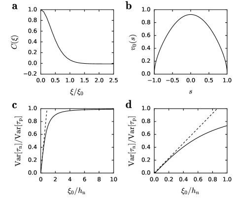
Figure 7: Numerical evaluation of Eq.24. (a) Correlation function. (b) First eigenfunction of the elastic problem. (c) Normalized variance of the nucleation strength $\tau_{\mathrm{n}}$. (d) Zoom over $\xi_{0}<h_{\mathrm{n}}$. Dashed line in (c,d) represents

References

- Amon et al. (2017) Amon, A., Blanc, B., Géminard, J.C., 2017. Avalanche precursors in a frictional model. Physical Review E 96, 033004. URL: https://link.aps.org/doi/10.1103/PhysRevE.96.033004, doi:10.1103/PhysRevE.96.033004.
- Amontons (1699) Amontons, G., 1699. De la résistance causée dans les machines. Memoires de l’Academie Royale A , 275–282.
- Ampuero et al. (2006) Ampuero, J.P., Ripperger, J., Mai, P.M., 2006. Properties of Dynamic Earthquake Ruptures With Heterogeneous Stress Drop, in: Earthquakes: Radiated Energy and the Physics of Faulting. American Geophysical Union, Washington, DC, pp. 255–261. URL: https://resolver.caltech.edu/CaltechAUTHORS:20120830-075047141.
- Ampuero and Rubin (2008) Ampuero, J.P., Rubin, A.M., 2008. Earthquake nucleation on rate and state faults – Aging and slip laws. Journal of Geophysical Research: Solid Earth 113. URL: https://agupubs.onlinelibrary.wiley.com/doi/abs/10.1029/2007JB005082, doi:10.1029/2007JB005082.
- Andrews (1976) Andrews, D.J., 1976. Rupture velocity of plane strain shear cracks. Journal of Geophysical Research (1896-1977) 81, 5679–5687. URL: https://agupubs.onlinelibrary.wiley.com/doi/abs/10.1029/JB081i032p05679, doi:10.1029/JB081i032p05679.
- Barras et al. (2019) Barras, F., Aghababaei, R., Molinari, J.F., 2019. Onset of sliding across scales: How the contact topography impacts frictional strength. arXiv:1910.11280 [cond-mat, physics:physics] URL: http://arxiv.org/abs/1910.11280. arXiv: 1910.11280.
- Bayart et al. (2016) Bayart, E., Svetlizky, I., Fineberg, J., 2016. Fracture mechanics determine the lengths of interface ruptures that mediate frictional motion. Nature Physics 12, 166–170. URL: http://www.nature.com/nphys/journal/v12/n2/abs/nphys3539.html, doi:10.1038/nphys3539.
- Ben-David and Fineberg (2011) Ben-David, O., Fineberg, J., 2011. Static Friction Coefficient Is Not a Material Constant. Physical Review Letters 106, 254301. URL: https://link.aps.org/doi/10.1103/PhysRevLett.106.254301, doi:10.1103/PhysRevLett.106.254301.
- Beroza and Ellsworth (1996) Beroza, G.C., Ellsworth, W.L., 1996. Properties of the seismic nucleation phase. Tectonophysics 261, 209–227. URL: http://www.sciencedirect.com/science/article/pii/0040195196000674, doi:10.1016/0040-1951(96)00067-4.
- Bilby and Eshelby (1968) Bilby, B., Eshelby, J., 1968. Disclocations and theory of fracture, in: Liebowitz, H. (Ed.), Fracture, An Advanced Treatise. Academic, San Diego. volume 1, pp. 99–182.
- Bowden and Tabor (1950) Bowden, F., Tabor, D., 1950. The Friction and Lubrication of Solids. Clarendon Press, Oxford, UK.
- Breitenfeld and Geubelle (1998) Breitenfeld, M.S., Geubelle, P.H., 1998. Numerical analysis of dynamic debonding under 2D in-plane and 3D loading. International Journal of Fracture 93, 13–38. URL: https://link.springer.com/article/10.1023/A:1007535703095, doi:10.1023/A:1007535703095.
- Campillo and Ionescu (1997) Campillo, M., Ionescu, I.R., 1997. Initiation of antiplane shear instability under slip dependent friction. Journal of Geophysical Research: Solid Earth 102, 20363–20371. URL: https://agupubs.onlinelibrary.wiley.com/doi/abs/10.1029/97JB01508, doi:10.1029/97JB01508.
- Carlson and Langer (1989) Carlson, J.M., Langer, J.S., 1989. Properties of earthquakes generated by fault dynamics. Physical Review Letters 62, 2632–2635. URL: https://link.aps.org/doi/10.1103/PhysRevLett.62.2632, doi:10.1103/PhysRevLett.62.2632.
- Coulomb (1785) Coulomb, C., 1785. Théorie des machines simples, en ayant regard au frottement de leurs parties, et à la roideur des cordages. Memoires deMathematique et de Physique de l’Academie Royale , 161–342.
- Dansereau et al. (2019) Dansereau, V., Démery, V., Berthier, E., Weiss, J., Ponson, L., 2019. Collective Damage Growth Controls Fault Orientation in Quasibrittle Compressive Failure. Physical Review Letters 122, 085501. URL: https://link.aps.org/doi/10.1103/PhysRevLett.122.085501, doi:10.1103/PhysRevLett.122.085501.
- Dieterich (1979) Dieterich, J.H., 1979. Modeling of rock friction: 1. Experimental results and constitutive equations. Journal of Geophysical Research: Solid Earth 84, 2161–2168. URL: https://agupubs.onlinelibrary.wiley.com/doi/abs/10.1029/JB084iB05p02161, doi:10.1029/JB084iB05p02161.
- Dieterich and Kilgore (1994) Dieterich, J.H., Kilgore, B.D., 1994. Direct observation of frictional contacts: New insights for state-dependent properties. pure and applied geophysics 143, 283–302. URL: https://doi.org/10.1007/BF00874332, doi:10.1007/BF00874332.
- Garagash and Germanovich (2012) Garagash, D.I., Germanovich, L.N., 2012. Nucleation and arrest of dynamic slip on a pressurized fault. Journal of Geophysical Research: Solid Earth 117. URL: https://agupubs.onlinelibrary.wiley.com/doi/abs/10.1029/2012JB009209, doi:10.1029/2012JB009209.
- Geubelle and Rice (1995) Geubelle, P.H., Rice, J.R., 1995. A spectral method for three-dimensional elastodynamic fracture problems. Journal of the Mechanics and Physics of Solids 43, 1791–1824. URL: http://www.sciencedirect.com/science/article/pii/002250969500043I, doi:10.1016/0022-5096(95)00043-I.
- Geus et al. (2019) Geus, T.W.J.d., Popović, M., Ji, W., Rosso, A., Wyart, M., 2019. How collective asperity detachments nucleate slip at frictional interfaces. Proceedings of the National Academy of Sciences 116, 23977–23983. URL: https://www.pnas.org/content/116/48/23977, doi:10.1073/pnas.1906551116.
- Greenwood et al. (1966) Greenwood, J.A., Williamson, J.B.P., Bowden, F.P., 1966. Contact of nominally flat surfaces. Proceedings of the Royal Society of London. Series A. Mathematical and Physical Sciences 295, 300–319. URL: https://royalsocietypublishing.org/doi/abs/10.1098/rspa.1966.0242, doi:10.1098/rspa.1966.0242.
- Grigoriu (1995) Grigoriu, M., 1995. Applied non-Gaussian processes: examples, theory, simulation, linear random vibration, and MATLAB solutions. PTR Prentice Hall, Englewood Cliffs, NJ. Http://newcatalog.library.cornell.edu/catalog/2681811.
- Hinkle et al. (2020) Hinkle, A.R., Nöhring, W.G., Leute, R., Junge, T., Pastewka, L., 2020. The emergence of small-scale self-affine surface roughness from deformation. Science Advances 6, eaax0847. URL: https://advances.sciencemag.org/content/6/7/eaax0847, doi:10.1126/sciadv.aax0847.
- Hyun and Robbins (2007) Hyun, S., Robbins, M.O., 2007. Elastic contact between rough surfaces: Effect of roughness at large and small wavelengths. Tribology International 40, 1413–1422. URL: http://www.sciencedirect.com/science/article/pii/S0301679X07000369, doi:10.1016/j.triboint.2007.02.003.
- Kammer and McLaskey (2019) Kammer, D.S., McLaskey, G.C., 2019. Fracture energy estimates from large-scale laboratory earthquakes. Earth and Planetary Science Letters 511, 36–43. URL: http://www.sciencedirect.com/science/article/pii/S0012821X19300573, doi:10.1016/j.epsl.2019.01.031.
- Kammer et al. (2015) Kammer, D.S., Radiguet, M., Ampuero, J.P., Molinari, J.F., 2015. Linear Elastic Fracture Mechanics Predicts the Propagation Distance of Frictional Slip. Tribology Letters 57, 23. URL: https://doi.org/10.1007/s11249-014-0451-8, doi:10.1007/s11249-014-0451-8.
- Ke et al. (2018) Ke, C.Y., McLaskey, G.C., Kammer, D.S., 2018. Rupture Termination in Laboratory-Generated Earthquakes. Geophysical Research Letters 45, 12,784–12,792. URL: https://agupubs.onlinelibrary.wiley.com/doi/abs/10.1029/2018GL080492, doi:10.1029/2018GL080492.
- Ke et al. (2019) Ke, C.Y., McLaskey, G.C., Kammer, D.S., 2019. Analytical Crack Model Inferred from Contained Laboratory-Generated Earthquakes. preprint DOI: 10.31223/osf.io/ur2pf. EarthArXiv. URL: https://osf.io/ur2pf.
- Latour et al. (2013) Latour, S., Schubnel, A., Nielsen, S., Madariaga, R., Vinciguerra, S., 2013. Characterization of nucleation during laboratory earthquakes. Geophysical Research Letters 40, 5064–5069. URL: https://agupubs.onlinelibrary.wiley.com/doi/abs/10.1002/grl.50974, doi:10.1002/grl.50974.
- Li and Kim (2008) Li, Q., Kim, K.S., 2008. Micromechanics of friction: effects of nanometre-scale roughness. Proceedings of the Royal Society A: Mathematical, Physical and Engineering Sciences 464, 1319–1343. URL: https://royalsocietypublishing.org/doi/10.1098/rspa.2007.0364, doi:10.1098/rspa.2007.0364.
- Li et al. (2013) Li, Q., Popov, M., Dimaki, A., Filippov, A.E., Kürschner, S., Popov, V.L., 2013. Friction Between a Viscoelastic Body and a Rigid Surface with Random Self-Affine Roughness. Physical Review Letters 111, 034301. URL: https://link.aps.org/doi/10.1103/PhysRevLett.111.034301, doi:10.1103/PhysRevLett.111.034301.
- Li et al. (2018) Li, Z., Pastewka, L., Szlufarska, I., 2018. Chemical aging of large-scale randomly rough frictional contacts. Physical Review E 98, 023001. URL: https://link.aps.org/doi/10.1103/PhysRevE.98.023001, doi:10.1103/PhysRevE.98.023001.
- Lyashenko et al. (2013) Lyashenko, I.A., Pastewka, L., Persson, B.N.J., 2013. Comment on “Friction Between a Viscoelastic Body and a Rigid Surface with Random Self-Affine Roughness”. Physical Review Letters 111, 189401. URL: https://link.aps.org/doi/10.1103/PhysRevLett.111.189401, doi:10.1103/PhysRevLett.111.189401.
- McLaskey (2019) McLaskey, G.C., 2019. Earthquake Initiation From Laboratory Observations and Implications for Foreshocks. Journal of Geophysical Research: Solid Earth 124, 12882–12904. URL: https://agupubs.onlinelibrary.wiley.com/doi/abs/10.1029/2019JB018363, doi:10.1029/2019JB018363.
- Noda et al. (2013) Noda, H., Nakatani, M., Hori, T., 2013. Large nucleation before large earthquakes is sometimes skipped due to cascade-up—Implications from a rate and state simulation of faults with hierarchical asperities. Journal of Geophysical Research: Solid Earth 118, 2924–2952. URL: http://agupubs.onlinelibrary.wiley.com/doi/abs/10.1002/jgrb.50211, doi:10.1002/jgrb.50211. _eprint: https://onlinelibrary.wiley.com/doi/pdf/10.1002/jgrb.50211.
- Pei et al. (2005) Pei, L., Hyun, S., Molinari, J.F., Robbins, M.O., 2005. Finite element modeling of elasto-plastic contact between rough surfaces. Journal of the Mechanics and Physics of Solids 53, 2385–2409. URL: http://www.sciencedirect.com/science/article/pii/S0022509605001225, doi:10.1016/j.jmps.2005.06.008.
- Persson (2001) Persson, B.N.J., 2001. Theory of rubber friction and contact mechanics. The Journal of Chemical Physics 115, 3840–3861. URL: https://aip.scitation.org/doi/10.1063/1.1388626, doi:10.1063/1.1388626.
- Pilvelait et al. (2020) Pilvelait, T., Dillavou, S., Rubinstein, S.M., 2020. Influences of microcontact shape on the state of a frictional interface. Physical Review Research 2, 012056. URL: https://link.aps.org/doi/10.1103/PhysRevResearch.2.012056, doi:10.1103/PhysRevResearch.2.012056.
- Popova and Popov (2015) Popova, E., Popov, V.L., 2015. The research works of Coulomb and Amontons and generalized laws of friction. Friction 3, 183–190. URL: https://doi.org/10.1007/s40544-015-0074-6, doi:10.1007/s40544-015-0074-6.
- Rabinowicz (1992) Rabinowicz, E., 1992. Friction coefficients of noble metals over a range of loads. Wear 159, 89–94. URL: http://www.sciencedirect.com/science/article/pii/004316489290289K, doi:10.1016/0043-1648(92)90289-K.
- Rabinowicz (1995) Rabinowicz, E., 1995. Friction and wear of materials. 2nd ed ed., Wiley, New York.
- Ray and Viesca (2017) Ray, S., Viesca, R.C., 2017. Earthquake Nucleation on Faults With Heterogeneous Frictional Properties, Normal Stress. Journal of Geophysical Research: Solid Earth 122, 8214–8240. URL: https://agupubs.onlinelibrary.wiley.com/doi/abs/10.1002/2017JB014521, doi:10.1002/2017JB014521.
- Ray and Viesca (2019) Ray, S., Viesca, R.C., 2019. Homogenization of fault frictional properties. Geophysical Journal International 219, 1203–1211. URL: https://academic.oup.com/gji/article/219/2/1203/5533328, doi:10.1093/gji/ggz327.
- Rice and Ruina (1983) Rice, J.R., Ruina, A.L., 1983. Stability of Steady Frictional Slipping. Journal of Applied Mechanics 50, 343–349. URL: https://asmedigitalcollection.asme.org/appliedmechanics/article/50/2/343/389397/Stability-of-Steady-Frictional-Slipping, doi:10.1115/1.3167042.
- Rubin and Ampuero (2005) Rubin, A.M., Ampuero, J.P., 2005. Earthquake nucleation on (aging) rate and state faults. Journal of Geophysical Research: Solid Earth 110. URL: https://agupubs.onlinelibrary.wiley.com/doi/abs/10.1029/2005JB003686, doi:10.1029/2005JB003686.
- Rubino et al. (2017) Rubino, V., Rosakis, A.J., Lapusta, N., 2017. Understanding dynamic friction through spontaneously evolving laboratory earthquakes. Nature Communications 8, 1–13. URL: https://www.nature.com/articles/ncomms15991/, doi:10.1038/ncomms15991.
- Rubinstein et al. (2007) Rubinstein, S.M., Cohen, G., Fineberg, J., 2007. Dynamics of Precursors to Frictional Sliding. Physical Review Letters 98, 226103. URL: https://link.aps.org/doi/10.1103/PhysRevLett.98.226103, doi:10.1103/PhysRevLett.98.226103.
- Ruina (1983) Ruina, A., 1983. Slip instability and state variable friction laws. Journal of Geophysical Research: Solid Earth 88, 10359–10370. URL: https://agupubs.onlinelibrary.wiley.com/doi/abs/10.1029/JB088iB12p10359, doi:10.1029/JB088iB12p10359.
- Sahli et al. (2018) Sahli, R., Pallares, G., Ducottet, C., Ali, I.E.B., Akhrass, S.A., Guibert, M., Scheibert, J., 2018. Evolution of real contact area under shear and the value of static friction of soft materials. Proceedings of the National Academy of Sciences 115, 471–476. URL: https://www.pnas.org/content/115/3/471, doi:10.1073/pnas.1706434115.
- Savio et al. (2016) Savio, D., Pastewka, L., Gumbsch, P., 2016. Boundary lubrication of heterogeneous surfaces and the onset of cavitation in frictional contacts. Science Advances 2, e1501585. URL: https://advances.sciencemag.org/content/2/3/e1501585, doi:10.1126/sciadv.1501585.
- Sokoloff (2001) Sokoloff, J.B., 2001. Static Friction between Elastic Solids due to Random Asperities. Physical Review Letters 86, 3312–3315. URL: https://link.aps.org/doi/10.1103/PhysRevLett.86.3312, doi:10.1103/PhysRevLett.86.3312.
- Spencer and Tysoe (2015) Spencer, N.D., Tysoe, W.T., 2015. The cutting edge of tribology: a decade of progress in friction, lubrication, and wear. World Scientific, [Hackensack], New Jersey. OCLC: ocn907104207.
- Svetlizky et al. (2020) Svetlizky, I., Albertini, G., Cohen, G., Kammer, D.S., Fineberg, J., 2020. Dynamic fields at the tip of sub-Rayleigh and supershear frictional rupture fronts. Journal of the Mechanics and Physics of Solids 137, 103826. URL: http://www.sciencedirect.com/science/article/pii/S0022509619308282, doi:10.1016/j.jmps.2019.103826.
- Svetlizky and Fineberg (2014) Svetlizky, I., Fineberg, J., 2014. Classical shear cracks drive the onset of dry frictional motion. Nature 509, 205–208. URL: https://www.nature.com/articles/nature13202, doi:10.1038/nature13202.
- Thomas (1999) Thomas, T.R., 1999. Rough surfaces. 2. ed ed., Imperial College Press, London. OCLC: 632713233.
- Uenishi and Rice (2003) Uenishi, K., Rice, J.R., 2003. Universal nucleation length for slip-weakening rupture instability under nonuniform fault loading. Journal of Geophysical Research: Solid Earth 108. URL: https://agupubs.onlinelibrary.wiley.com/doi/abs/10.1029/2001JB001681, doi:10.1029/2001JB001681.
- Yastrebov et al. (2015) Yastrebov, V.A., Anciaux, G., Molinari, J.F., 2015. From infinitesimal to full contact between rough surfaces: Evolution of the contact area. International Journal of Solids and Structures 52, 83–102. URL: http://www.sciencedirect.com/science/article/pii/S0020768314003667, doi:10.1016/j.ijsolstr.2014.09.019.