The variable and non-variable X-ray absorbers in Compton-thin type-II Active Galactic Nuclei

Abstract

We have conducted an extensive X-ray spectral variability study of a sample of 20 Compton-thin type II galaxies using broad band spectra from XMM-Newton, Chandra, and Suzaku. The aim is to study the variability of the neutral intrinsic X-ray obscuration along the line of sight and investigate the properties and location of the dominant component of the X-ray-obscuring gas. The observations are sensitive to absorption columns of $N_{\rm H}\sim 10^{20.5-24}\rm\,\,{\rm cm^{-2}}$ of fully- and partially-covering neutral and/or lowly-ionized gas on timescales spanning days to well over a decade. We detected variability in the column density of the full-covering absorber in 7/20 sources, on timescales of months-years, indicating a component of compact-scale X-ray-obscuring gas lying along the line of sight of each of these objects. Our results imply that torus models incorporating clouds or overdense regions should account for line of sight column densities as low as $\sim$ a few $\times 10^{21}$ cm^-2. However, 13/20 sources yielded no detection of significant variability in the full-covering obscurer, with upper limits to ${\Delta}N_{\rm H}$ spanning $10^{21-23}$ cm^-2. The dominant absorbing media in these systems could be distant, such as kpc-scale dusty structures associated with the host galaxy, or a homogeneous medium along the line of sight. Thus, we find that overall, strong variability in full-covering obscurers is not highly prevalent in Compton-thin type IIs, at least for our sample, in contrast to previous results in the literature. Finally, 11/20 sources required a partial-covering, obscuring component in all or some of their observations, consistent with clumpy near-Compton-thick compact-scale gas.

1. INTRODUCTION

It is now generally agreed that the main source of energy of an active galactic nucleus (AGN) is the accretion of matter onto a supermassive black hole (SMBH). However, it is still unknown how gas located at kpc scales in the host galaxy loses its angular momentum and falls into the gravitational potential well of the SMBH at sub-pc scales and thereby powers the central engine. Galactic-scale bars, circumnuclear disks at scales of a few hundred parsecs, and circumnuclear gas structures at scales of parsecs, in the near vicinity of the SMBH, are each believed to play roles in transferring matter ultimately from large distances into the SMBH accretion disk.

The observed type 1/2 Seyfert dichotomy in the optical band led to orientation-dependent unification schemes: all AGN function similarly, and the different spectral classifications of AGN arise only due to the different lines of sight toward the central engine (Antonucci & Miller, 1985). When we have a direct unobscured view of the central engine, then the optical-UV spectra exhibit broad as well as narrow emission lines and the source is classified as a type 1–1.8 (collectively hereafter referred to as type I). On the other hand, if our line of sight to the central engine cuts across a dusty structure popularly known as a “torus”, the central engine is no longer visible directly and the optical-UV spectra we observe are characterized only by narrow emission lines. In such a case, the source is regarded as a type 1.9–2 (hereafter type II) AGN. Classically, the dusty torus was expected to extend to $\sim$pc scales — larger than the BLR but smaller than the NLR (e.g., Krolik & Begelman, 1988). The simplest configuration is an axisymmetric donut-shaped torus, but this notion was effectively a starting point for more complex models, and in recent decades the community has been probing the morphology, content, and radial extent of the circumnuclear gas (see e.g., the reviews by Bianchi et al., 2012a; Ramos Almeida & Ricci, 2017)

Firstly, the community has been accumulating evidence for optical-reddening dust and X-ray-obscuring gas (which can potentially be dusty or non-dusty) to exist across multiple distance scales from the SMBH. Inside the dust sublimation radius, and commensurate with the BLR, temporary X-ray obscuration can occur due to individual clouds (possibly BLR clouds themselves) transiting the line of sight (e.g., Risaliti et al., 2009, 2011). In addition, observations of ratios of $N_{\rm H}$ (as probed by X-rays) to V-band extinction $A_{\rm V}$ are found to be much greater — sometimes a couple orders of magnitude — than the Galactic ratio (Maiolino et al., 2001). Farther out, optical/IR reverberation monitoring indicates thermally-emitting dust on scales of light-weeks to light-months (see e.g., Suganuma et al., 2006). In addition, dusty gas on scales of parsecs to tens–hundreds of parsecs is revealed by IR interferometry (e.g., Kishimoto et al., 2009; Tristram et al., 2009); sub-mm observations also indicate dense molecular gas at these distance scales (e.g., Schinnerer et al., 2000; Boone et al., 2011; Gallimore et al., 2016; Imanishi et al., 2016, 2018; García-Burillo et al., 2016; Combes et al., 2019). These radial structures may potentially be connected: for example (Netzer & Laor, 1993) and (Elitzur, 2007) posit that material spanning both the dusty torus and (non-dusty) BLR forms a radially-continuous component (Toroidal Obscuring Region/BLR-Obscuring Region, or ”TOR/BOR”). Henceforth, in this paper, for simplicity, we refer to the “torus” as a synonym for “compact scale (less than 10 pc) X-ray-obscuring gas,” with the exact morphology and extent to be determined. Specifically, we focus on all X-ray-obscuring gas along the line of sight both inside and outside the dust sublimation radius, regardless of morphology.

Secondly, some components of circumnuclear gas may contain discrete clumps or filaments, and/or overdensities embedded in a continuous, lower-density medium, as opposed to having a one-component continuous, homogeneous structure; clumpy-torus models positing extended distributions of clouds (e.g., Elitzur & Shlosman, 2006; Risaliti et al., 2007; Nenkova et al., 2008; Hönig et al., 2013) are consequently finding observational support, particularly from X-ray spectral studies. For example, Risaliti et al. (2002) studied variability of line-of-sight, neutral, X-ray-obscuring column density $N_{\rm H}$ in a sample of Compton-thin and moderately Compton-thick type IIs. They detected almost ubiquitous (22/25 objects) variability in $N_{\rm H}$ on timescales of months to several years, with typical variations up to factors of $\sim 1.5-3$. Their analysis combined multiple single-epoch observations across a range of different X-ray missions. For a subsample of 11 sources the authors could detect relatively rapid variations ($\leq 1$ year), with obscuring columns typically varying by $10^{22}-10^{23}$ cm^-2. More recently, the community has used more continuous X-ray monitoring data (e.g., from Rossi X-ray Timing Explorer; RXTE) or single-epoch X-ray long-looks (with e.g., XMM-Newton or Suzaku) to track ingress/egress of individual clouds, finding support for clouds existing at radii spanning both inside and outside the dust sublimation radius (Lamer et al., 2003; Puccetti et al., 2007; Risaliti et al., 2009, 2011; Maiolino et al., 2010; Sanfrutos et al., 2013). Markowitz et al. (2014) (2014; hereafter MKN14) provided the first X-ray-based statistical support for the clumpy-torus model of Nenkova et al. (2008) by studying the obscuration variability of a sample of 55 type Is and Compton-thin type IIs using long-term RXTE monitoring. This variability database yielded a total of 12 full-covering eclipse events across eight objects. The event durations spanned hours to $>$ a year, with clouds’ column densities typically ($4-26$) $\times 10^{22}$ cm^-2, i.e., no full-covering Compton-thick eclipse events were observed. In seven objects, the clouds were inferred to be located at radial distances commensurate with the outer BLR or the inner dusty torus. MKN14 also provided the first X-ray-based probability estimates for witnessing eclipses in type I/II objects. Finally, infrared studies probing the dusty part of the obscurer also support clumpy-torus models, via spectral energy distribution modeling (Ramos Almeida et al., 2011, 2014), the co-existence of relatively hotter and cooler dust components in nearby AGN (Jaffe et al., 2004; Raban et al., 2009), and the range of 9.7 $\mu$m Si emission/absorption features spanned by type I and II Seyferts (Nikutta et al., 2009).

Both the dusty and non-dusty components of the torus are believed to play an active role in SMBH accretion, and hence, understanding the structure of the torus is essential for understanding both disk/SMBH fueling and orientation-dependent unification schemes. However, there are additional complications that simple orientation-dependent unification cannot easily explain. There is likely a dependence of the torus covering factor on luminosity or $\lambda_{\rm Edd}\equiv L_{\rm Bol}/L_{\rm Edd}$; relatively stronger radiation fields from the nucleus can clear out more obscuring material (Ricci et al., 2017b). In addition, there is support for the BLR to disappear towards low values of AGN bolometric luminosity, forming the ”true type 2” objects (Elitzur & Ho, 2009; Bianchi et al., 2012b). One might therefore refer to the ”torus” or ”TOR/BOR” component, but it is likely the case that its morphology and/or spatial extent do not remain the same from one object to the next. We reiterate that in this paper, we refer to the ”torus” just to indicate compact-scale circumnuclear gas, with the precise morphology and spatial extent still to be determined by the community (e.g., a TOR/BOR is just one possibility), the content (smooth, clumpy, or mixed) also to be determined, and with the assumption that even if it is present in all AGN, its morphology and extent are not guaranteed to be the same universally.

Yet another major complication for unification schemes is potential optical extinction and X-ray obscuration originating at length scales much greater than the compact torus, at 100s of pc to kpc, and due to dusty structures or lanes associated with the host galaxy. Optically-selected samples of Seyferts tend to yield a systematic dearth of type Is in relatively more edge-on systems, (Maiolino & Rieke, 1995; Lagos et al., 2011). Edge-on systems also tend to exhibit relatively stronger optical extinction (Driver et al., 2007; Shao et al., 2007). The expansive Hubble Space Telescope (HST) snapshot survey of over 250 nearby Seyfert and starburst galaxies performed by Malkan et al. (1998) (1998; hereafter MGT98) revealed an array of fine-scale dusty structures in galaxies’ centers. They (and others such as Prieto et al., 2014) concluded that type II Seyferts are intrinsically more likely to be hosted in galaxies with nuclear dust structures crossing the line of sight, potentially alleviating the requirement for a compact torus to explain extinction of BLR lines (a fundamental component of orientation-dependent unification schemes).

X-ray studies yield a similar picture: in some high-spatial resolution X-ray images of nearby AGN, we can resolve where dust lanes directly obscure soft X-ray diffuse emission (e.g., NGC 7582 and Cen A: Bianchi et al., 2007; Kraft et al., 2008). Moreover, Guainazzi et al. (2001) and Guainazzi et al. (2005) have compared X-ray obscuring columns with Balmer decrements or nuclear dust morphology in samples of Compton-thin and Compton-thick Seyferts. Their results support the notion (put forth by e.g., Matt, 2000) that Compton-thin type IIs tend to reside preferentially in galaxies with dusty nuclear environments on scales of $>$$\sim$ 0.1 kpc. However, Compton-thick obscuration does not seem highly affected by nuclear dust content and is likely due to a compact torus instead. Host galaxy characteristics — namely the chance of having or not having a dusty filament along the line of sight to the nucleus — can therefore potentially impact both optical spectral type and whether or not a source is perpetually Compton-thin obscured. Searching for time variability in X-ray obscuration can potentially provide clues to distinguish between obscuration due to a compact torus versus that from host galaxy structures. Therefore, the main goal of the present paper is to test this simplified model with X-ray monitoring data, wherein the location of the X-ray-obscuring gas can be discerned by the extent of the variability in the X-ray obscurer. A detection of variability on timescales of years or shorter would point to a clumpy structure very likely associated with the torus. A lack of variability on timescales of years and longer in a given object supports the notion that the dominant obscuring gas is more likely associated with host galaxy dusty structures.

The present paper is motivated in part by MKN14’s results on a subsample of eight type IIs monitored with RXTE: these objects’ X-ray column densities remained constant over timescales from 0.6 to 8.4 years. However, RXTE’s limited bandpass (no coverage $<2$ keV) meant that sensitivity in ${\Delta}N_{\rm H}$ in these objects was limited, with limits on variability spanning $0.6-9\times 10^{22}$ cm^-2. In contrast, XMM-Newton, Suzaku, and Chandra observations of type II Seyferts can provide comparably stronger sensitivity in ${\Delta}N_{\rm H}$, courtesy of their soft X-ray coverage.

In this paper we investigate the variability of the X-ray obscuration column density of a sample of perpetually X-ray-obscured type II AGN in the local Universe to address the question of ”What is the origin of perpetual Compton-thin X-ray obscuration in optical type IIs?” The rest of this paper is as follows: We present the sample and data reduction in Section 2, the spectral analysis in Section 3, the results for X-ray obscuration and its variability in Section 4, and we discuss physical interpretations in Section 5. Section 6 contains our main conclusions.

2. Sample selection, Observations and data reduction

2.1. The Sample selection and properties

2.1.1 Sample selection

The sample of Compton-thin type II (X-ray classification) sources was selected from the existing literature, with the constraint that each source must have at least two observations for a given instrument with a minimum time separation of two days (observations executed within two days of each other are almost always part of the same proposal/long-look). The X-ray spectra for the sources in the sample are obtained from XMM-Newton, Chandra, and Suzaku observatories that are in the HEASARC public archives as on 1 July 2017. Only the Seyfert sub-types 1.9-2 (as listed in NED), referred to as Compton-thin type II, are considered in this work. We obtained a final list of 20 sources (See Table 1 for details). We focus on optical type II Seyferts because they are more likely to be perpetually obscured in X-rays compared to type Is, and we reviewed the literature to ensure that each source in our sample is indeed perpetually X-ray-obscured. Our sample is not intended to be a complete sample (for instance, very roughly $10\%$ of type IIs have values of $N_{\rm H}$ below $10^{21}$ cm^-2, e.g., Bassani et al., 1999), but it is an exploratory sample for expanding our knowledge on variability or lack thereof in the X-ray obscurers of type IIs. We focus on relatively X-ray bright objects (average observed 2–10 keV fluxes brighter than typically a few $\times$$10^{-12}$ erg cm^-2 s^-1 to ensure adequate signal-to-noise within each observation). We exclude Compton-thick-obscured AGN, as their X-ray spectra are best studied with bandpasses extending above 10 keV, such as NuSTAR. However, we are clearly sensitive to potentially detecting any Compton-thin to -thick transitions (or vice versa), though as we note below, none were observed.

2.1.2 Activity properties

Optical spectral classifications are listed in Table 1. Some of the sources are not Seyfert galaxies, such as Cen A or Cyg A, which host radio jets, or NGC 1052, which is an X-ray-obscured LINER exhibiting broad polarized lines. We note as a caveat that even if the torus exists in all objects, its morphology and spatial extent (scaled relative to $M_{\rm BH}$) may very well likely differ between different activity classes, e.g., radio-loud versus radio-quiet objects; a detailed discussion of the impact of the presence/lack of a jet on torus morphology is beyond the scope of the current paper. Ten sources have been confirmed to harbor hidden BLRs, five using scattered polarized emission (denoted by “$1H$” in Table 1) in which case a compact torus is likely to exist along the line of sight. The other five (denoted by “$1I$”) have detections of broad recombination lines in the IR (e.g., Nagar et al., 2002); on that basis alone, it is not clear where the absorbing gas lies or how much of the total observed column is due to the host galaxy versus any putative torus; a potential observation of variability in $N_{\rm H}$ could confirm the existence of the compact torus along the line of sight in such cases.

2.1.3 Host galaxy properties of the sample

The objects in our sample are known to span a range of host galaxy properties. A majority of our sample have been studied in the snapshot survey by Malkan et al. (1998): eight have dust lanes crossing the line of sight to the nucleus or just offset from it; four have filamentary/wispy or irregular dusty structures. Sixteen of our objects are hosted in spirals, with semi-major/minor axis ratios (as listed on NED) indicating disk inclinations spanning roughly 30–75 degrees from the plane of the sky. The other four are hosted in ellipticals (Cen A, Cyg A, NGC 1052, and NGC 6251).

2.2. Observations and data reduction

To effectively detect any Compton-thin variable obscuration in the X-rays, the best instruments to use are the EPIC cameras aboard XMM-Newton, the XIS detectors aboard Suzaku and the ACIS detectors aboard Chandra, as they each provide a broadband spectral view in the energy range $\sim 0.5-10\rm\,\,{\rm keV}$, crucial for tracking the neutral absorption roll-over. We describe below the methods employed to reprocess and clean the X-ray spectral data obtained from these telescopes.

2.2.1 XMM-Newton

The EPIC-pn data from XMM-Newton were reduced using the scientific analysis system (SAS) software (version 15) with the task epchain and using the latest calibration database available at the time we carried out the data reduction. We used EPIC-pn data because of its higher signal to noise ratio as compared to MOS. We filtered the EPIC-pn data for particle background counts using a rate cutoff of $<1$ ct s^-1 for photons $>10\rm\,\,{\rm keV}$, and created time-averaged source and background spectra, as well as the response matrix function (RMF) and auxiliary response function (ARF) for each observation using the xmmselect command in SAS. The source regions were selected with a circle radius of $40"$ centred on the centroid of the source. The background regions were selected with a circle of $40"$ located on the same CCD, but located a few arc-minutes away from the source and avoiding X-ray-emitting point sources. Spectra were accumulated using pattern $0-4$. We found that the sources NGC 4258 and Cyg A are extended in the EPIC-pn CCD image, possibly due to the resolved, diffuse stellar emission in the former, and due to diffuse X-ray emission from intercluster gas in the latter.

We checked for possible pile up in the sources using the command epatplot in SAS, and found that the spectra of the source Cen A are piled up. For Cen A we thus used an annular extraction region for the source, with an inner radius of $20"$ and outer radius $40"$ to minimize pile-up. We did not detect significant pile up in the EPIC-pn spectra of the other sources.

2.2.2 Chandra

We considered Advanced CCD Imaging Spectrometer (ACIS-I and ACIS-S) data as well as 0th-order High-Energy Transmission Grating Spectrometer (HETGS) data. All Chandra data were reprocessed using the command chandra_repro in the CIAO software (version 4.7.1) and using the latest calibration database. Source regions were selected using a circle of radius 4.0”. The background regions were selected using a circle of radius of 4.0” on the same CCD as the source, but away from the source. We detected pileup (ranging from severe to mild) in the ACIS CCD spectra for the sources IRAS F05189$-$2524, NGC 1052, NGC 5252, NGC 5506, NGC 6251, NGC 6300, NGC 7172, NGC 7582, Mkn 348, NGC 4507 and MCG$-$5-23-16. Excluding a central circular region from the source image, as is typically done to exclude piled up data in XMM-Newton EPIC spectra, may lead to issues with the ARF in the Chandra spectra, and so that method was avoided. We instead use the pile-up kernel in the spectral fitting codes to model the pile up. In those cases where the pile-up is too severe to be modeled by such a kernel (such as in Cen A), we excluded those observations from our study.

2.2.3 Suzaku

The Suzaku observations were performed using the X-ray Imaging Spectrometer (XIS) (Koyama et al., 2007) and Hard X-ray Detector (HXD) (Takahashi et al., 2007). The XIS observations were obtained in both the $3\times 3$ and $5\times 5$ data modes. The aepipeline tool was used to reprocess and clean the unfiltered event files and to create the cleaned event files. In all observations, for both the XIS0 and XIS3 (front-illuminated CCD) and for XIS1 (back-illuminated CCD), we extracted the source spectra for each observation from the filtered event lists using a $120$” circular region centered at the source position. We also extracted the corresponding background spectral data using four circular regions of $120{\rm~{}arcsec}$ radii, a few arcminutes away from the source region and avoiding X-ray-emitting point sources. There are only a few cases of pile-up in Suzaku observations; we excluded those centrally-located pixels for which pile-up exceeded a threshold of $4\%$. During spectral fits, we did not co-add the front-illuminated XIS spectra, instead fitting them separately.

3. Spectral analysis

We used ISIS (Interactive Spectral Interpretation System) software (Houck & Denicola, 2000) for spectral fitting carried out in this work. The XMM-Newton spectra were grouped by a minimum of 20 counts per channel and a maximum of five resolution elements using the command Specgroup in SAS. The Chandra and Suzaku spectra were grouped by a minimum of 20 counts per channel in ISIS. As described below, we have carried out iterative steps to systematically fit all the X-ray spectra and account for both soft- and hard-band components while obtaining precise estimates of the intrinsic neutral absorption column densities. In this section we first describe the models we used to fit the spectra and then elucidate stepwise the fitting procedure that we employed.

We started from a “baseline” model that follows (using ISIS notation)

TBabs(1) $\times$ (apec(1)+ apec(2) + powerlaw(1) + zTBabs(1) $\times$ (powerlaw(2) + pexmon(1)+ zgauss)).

If an additional partial-covering absorption component is required by the data, then our model became

TBabs(1) $\times$ (apec(1) + apec(2)+ powerlaw(1) + zTBabs(1) $\times$ zpcfabs(1) $\times$ (powerlaw(2) + pexmon(1) + zgauss )).

The TBabs and zTBabs components model the Galactic and intrinsic fully-covering neutral absorption column, respectively. zpcfabs models the partial covering absorption component, if significantly detected. The primary, hard power law (powerlaw(2)) models the Compton-upscattered emission from a hot optically-thin corona in the central AGN. In addition we have tested for the possible presence of warm ionized absorbers (Blustin et al., 2005; Laha et al., 2014) using warm-abs model (Kallman & Bautista, 2001) in ISIS, but did not detect any statistically significant warm absorption in any of the sources in the sample. The best fit models and details of the analysis for every source have been reported in Appendix A.

The soft band may contain emission from thermal plasma, which could be due to star formation (e.g., Turner et al., 1997). Continuum emission due to scattering of the primary X-ray emission in Compton-thin circumnuclear gas out to $\sim$ a kpc (e.g., Cappi et al., 2006; Ueda et al., 2007; Awaki et al., 2008; Ricci et al., 2017a) is also expected. There also likely exist signatures of gas being photo-ionized and photo-excited, namely soft emission lines and radiative recombination continuum (RRC) features, likely originating in the AGN-illuminated regions of the Narrow Line Region (e.g., Bianchi et al., 2006; Guainazzi & Bianchi, 2007). Indeed, 12 of our sources are contained in the CIELO-AGN sample of Guainazzi & Bianchi (2007); however, such features are typically identified by gratings observations and will be blurred at CCD resolution, so we do not explicitly model them here.

We use one (or two, if necessary) apec component(s) to model any thermal emission. powerlaw(1) denotes the secondary (soft) power law to model the scattered emission, with the expectation that the normalization of the soft power law will be of the order $\lesssim 1\%$ that of the hard power law, approximately. We first attempt to fit with the value of soft photon index $\Gamma_{\rm SX}$ tied to that of the primary (hard) X-ray power law but only if a significant improvement in fit results from thawing $\Gamma_{\rm SX}$ then we do so. As mentioned earlier, the soft-band power-law is expected to model scattered nuclear emission and in the ideal case, the photon indices of the soft and hard power laws should match. However, there can be numerous potential reasons for a mismatch, including that the current value of the hard X-ray power-law photon index may be different from the long-term averaged photon index scattered off extended diffuse gas, or there may be blending with emission from other components, such as unresolved point sources (ULXs).

Although the baseline model gives a reasonable fit in most cases, it is definitely not the case that a common baseline model can be applied equally to all objects/observations. For a given instrument (e.g., XMM-Newton), some objects’ spectra require only one apec component; others require two. Relativistically broad Fe K emission lines were detected only in two sources, MCG–5-23-16 and Fairall 49, and for simplicity we have used diskline to model them (See Appendix A for details of the fits).

In addition, for a given object, different instruments have different apertures, different responses/effective areas, etc., so some components (apec, narrow Fe K line) detected in one instrument for a given object are not detected in other instruments. As one example, the Chandra observations for the sources NGC 2992 and NGC 7314 did not require any apec components, but the XMM-Newton and Suzaku observations for the same sources required them. The goodness of fit upon adding a new model component has been tested both using $\,\Delta\chi^{2}$ and Ftest, requiring a $>5\sigma$ improvement in statistics to consider the new model component as required in the fit.

Ideally, we would have liked to perform, for each object/instrument combination, joint fitting in which we can have certain parameters freed but tied across all spectral fits (power-law photon indices, apec temperatures, etc.), but for practical reasons that could not be done due to the huge computational power required (especially for those objects with multiple Suzaku datasets). We also note that not all objects in the sample adhere to a common “baseline” model, and not all objects follow the same spectral variability behavior in soft and hard x-ray bands. For example, given that soft-band emission likely originates in diffuse gas, we do not expect it to exhibit variability on timescales of $\sim$ years and shorter. However in several object/instrument cases we did find strong evidence for soft-band variability; keeping soft-band parameters frozen resulted in poor fits in these cases: the XMM-Newton spectra of MCG–5-23-16, NGC 526a, NGC 2992, and NGC 7314, and the Chandra spectra of NGC 526a (See the spectral overplots in Appendix Fig 1-20). For example, in the first XMM-Newton observation of NGC 2992 (denoted as X-1), the entire continuum (except for the narrow Fe line flux, which is $\sim$ constant) is higher than for all the subsequent XMM-Newton observations. There could be several possible reasons: a leaky, patchy absorber which obscures the AGN and which has changed its covering fraction, a sudden spurt in stellar emission, or flaring emission from a transient point source such as a ULX. A detailed study of the causes behind each of these soft-band spectral variations would require high spatial resolution to separate out the AGN, stellar emission, other point sources, etc., and is therefore beyond the scope of this paper. At any rate, consequently, we adopt a two-step system: We first fit each observation separately, then for each object/instrument combination, we adopt the average values of all soft-band component parameters and freeze them during a second round of fits. While adopting this process we note as caveats that 1. different spectra can have different statistical weights and 2. freezing some parameters may shrink some error bars on fitted $N_{\rm H}$ values.

There is also the issue of the Compton reflection hump (hereafter CRH). The CRH is detected and mostly well constrained in individual Suzaku observations due to its broadband $0.3-40\rm\,\,{\rm keV}$ coverage, but remains unconstrained for the XMM-Newton or Chandra observations — meaning that CRH reflection strength and hard X-ray power-law parameters (which can in turn impact modeling of $N_{\rm H}$) cannot be unambiguously and independently constrained in $80\%$ of the observations involved in this work. We thus started our analysis for each object with Suzaku spectra and then applied that model to XMM-Newton and Chandra. We note here that for all the 20 sources in our sample we have at least one Suzaku observation, and hence we could use this approach for all of the sources.

We use pexmon to model the CRH and narrow Fe K emission line simultaneously. However, we need to understand how the CRH has varied with time for each object, in order to know which parameter values of the pexmon component to use for cases with multiple Suzaku observations. For simplicity, we consider two scenarios: 1. The CRH remains constant in absolute normalization with time, irrespective of the hard X-ray power-law $\Gamma$ and flux, and 2. The CRH responds instantaneously to the hard X-ray powerlaw variations (relative normalization constant). There are 8 sources for which there are multiple Suzaku observations and 12 sources with only one. For the 12 sources with only one Suzaku observation we have used the best fit pexmon values from that observation and assumed it to remain constant in absolute normalization in the XMM-Newton and Chandra observations, as there is no way to rule out or vindicate any of the above scenarios with the XMM-Newton or Chandra data. For the seven sources with multiple Suzaku observations (excluding Cen A, which lacks any CRH detected to date), we investigated potential CRH variability. After obtaining a broad-band best fit to each Suzaku observation, we calculated the absolute normalization of the pexmon component (simply the product of the model normalization and the reflection fraction $R$). For the sources MCG–5-23-16, NGC 4258, NGC 7314, and NGC 7582 the absolute normalization is consistent with being constant in time. This is consistent with the notion that at least in these objects, the CRH arises from a distant medium and does not vary over the timescales of our observations. For NGC 2110 the absolute normalization tracks the hard X-ray power-law normalization, suggesting that CRH flux tracks that of the coronal power law closely. For the sources NGC 2992 and NGC 5506, insufficient SNR or lack of significant variability in the hard X-ray powerlaw did not allow us to conclude the nature of CRH variability. Given the fact that a majority of these sources with multiple Suzaku observations are consistent with a constant-absolute normalization CRH, and since we lack information on the rest of the 12 objects, for simplicity and uniformity we assumed a constant-absolute normalization CRH for all the sources in our sample. In other words, we used the pexmon parameter values from the best-fit to S-1 (for a given object) and held those frozen when fitting the XMM-Newton and Chandra datasets for each of these objects.

In addition, we note that we did not detect any significant variability in the narrow Fe K$\alpha$ emission line (at $\sim 6.4\rm\,\,{\rm keV}$) flux in any of the objects. If we assume that the line arises from the same reprocessing medium as that responsible for the CRH, as is implicitly assumed when using pexmon, then this further supports the notion that reflected emission (CRH + Fe K line) is constant with time.

We note however, that for the high SNR XMM-Newton observations of MCG–5-23-16, we found that the narrow Fe K emission line and the CRH could not be simultaneously modeled by pexmon, implying e.g., that they arise from different reprocessing media, or there is a non-solar Fe abundance, In fact, we had to thaw the Fe abundance relative to solar, $Z_{\rm Fe}$, in pexmon to sub-solar values to obtain good fits: $Z_{\rm Fe}$ typically falls to $\sim 0.19$ and $\chi^{2}$ drops by at least $200$ in the X-2, X-3 and X-4 spectra.

The “second round” of fits are our best fits, listed in Tables 3 and 4. The error quoted on each parameter is the $90\%$ confidence interval for one free parameter. Note that we have only reported the errors for the soft X-ray parameters in Table 4 when they are kept free in the second round of fits, that is, when the fit requires a different value of these parameters than those of the average values.

4. Results

Table 3 lists the best fit parameters for the full and partial-covering line of sight absorbers, along with the $90\%$ confidence uncertainties. We first discuss the characteristics of the full-covering absorbers. The column densities of the full covering absorber in our sources have values spanning three orders of magnitude ($N_{\rm H}\sim 10^{20.5-23.5}$ cm^-2). We note that the distribution of mean values of $N_{\rm H}$ is roughly uniform, and does not show any clustering towards low or high values. We present light curves of $N_{\rm H}$ for all sources, shown in Fig. 1.

For a given source, we can search for variability in $N_{\rm H}$ by examining a single instrument only (to eliminate cross-instrument systematic effects), and in parallel, across different missions. The latter, however, is subject to cross-instrument calibration issues which are not straightforward to quantify and may depend on e.g., intrinsic spectral shape, the effect of differing apertures, etc., so cross-instrument comparisons of a given parameter must be taken with a grain of salt, and is discussed further in Section 4.2. Nonetheless, we note firstly that none of the sources exhibits any Compton-thin to -thick (or vice versa) transitions, considering both single instruments and across missions. Furthermore, variations in best-fit values of $N_{\rm H}$ are usually modest even over timescales of years: for any given object except Fairall 49, the maximum/minimum best-fit values of $N_{\rm H}$ typically never vary in ratio by more than $\sim$ 1.5–1.8 (within one instrument) or more than $\sim$ 2–5 (across all instruments for a given source). Fairall 49 is the standout exception, displaying an order of magnitude increase in $N_{\rm H}$ (this source is discussed further below).

As a caveat we remind the reader that in this work we are limited by the relatively sparse time sampling of the data, and we are not exploring variability on timescales less than $\sim$1 day in this work. This lack of sustained sampling means we are not as sensitive compared to RXTE in detecting complete (ingress-to-egress) eclipse events as detected by e.g., MKN14, Risaliti et al. (2011). Nonetheless we can probe up to timescales of nearly two decades, so we are probing a spatial extent similar to that of MKN14, although here we have greater sensitivity to smaller variations in $N_{\rm H}$, covering the range $\log(N_{\rm H}/\rm\,\,{\rm cm^{-2}})$ $\sim 20.5-23.5$.

4.1. Candidates for variability in $N_{\rm H}$ using single instruments

We select candidates for sources exhibiting variability in $N_{\rm H}$ (henceforth “variable-$N_{\rm H}$ sources”), but we first concentrate only on using single instruments for a given object. To be classified in this category, a given object/instrument combination must exhibit variability as follows:

• As a first cut, values of $N_{\rm H}$ between any two observations must differ by at least 3 times the 90% error in one parameter obtained from ISIS spectral fit (adopting a conservative criterion).

• A simple $\chi^{2}$ fit of the $N_{\rm H}$($t$) light curve against a constant must satisfy $\chi^{2}$/$dof$ $>5$.

• The X-ray spectra must be checked for possible model degeneracies that could influence $N_{\rm H}$ values; as described below, we perform Bayesian analysis with MultiNest to vet candidate-variable objects.

The first criterion lead to eight object/instrument combinations as candidates (here, X, S, and CA denote XMM-Newton, Suzaku, and Chandra-ACIS, respectively): Fairall 49/X, Cen A/S, MCG–5-23-16/X, MCG–5-23-16/S, NGC 2992/X, NGC 5252/CA, NGC 5506/X, and NGC 7582/X. We note that the XMM-Newton and Suzaku events of MCG–523-16 are different and not overlapping in time. All eight of the above events pass the second criterion, as testing against a constant yielded $\chi^{2}$/$dof$ $>5$. Two additional objects (NGC 4258/S and NGC 7582/X) pass this criterion but fail the first criterion (and partial coverers and/or low signal/noise may be at play), and hence we do not consider them further. Choosing a much less strict threshold for the first criterion, say 2 times the 90$\%$ errors, would have allowed only three more object/instrument combinations to pass this criterion. Similarly, choosing a lower threshold for $\chi^{2}/{dof}$ would not have significantly increased the number of objects passing the second criterion; lowering the threshold to 2.5, for example, would have allowed only two more object/instrument combinations to pass this criterion. We are thus confident that these two criteria are each reasonable in terms of separating outlying variability from the bulk of the distribution in which variability is not detected.

We then conducted Bayesian analysis to vet these candidates and verify that modest variations in $N_{\rm H}$ are not the result of degeneracies with other spectral component parameters. Specifically, we use the MultiNest nested-sampling algorithm (Skilling, 2004; Feroz et al., 2009) via the Bayesian X-ray Analysis (BXA) and PyMultiNest packages (Buchner et al., 2014) for XSPEC version 12.10.1f. Standard Markov Chain Monte Carlo (MCMC) algorithms form “chains” by comparing the likelihood of a test point against that of a new point randomly chosen from the prior distribution, and moves to the new point with a probability determined by the likelihoods. However, there may be convergence issues, in that parameter sub-spaces with non-negligible probabilities can potentially be under-explored by such chains. Nested sampling algorithms, including MultiNest, attempt to map out all of the most probable regions of parameter sub-space: it maintains a set of parameter vectors of fixed length, and removes the least-likely point, replacing it with a point with a higher likelihood, and thus shrinking the volume of parameter space. We use MultiNest version 3.10 with default arguments (400 live points, sampling efficiency of 0.8) set in BXA version 3.31. We paid particular attention to potential degeneracies between $N_{\rm H}$ and each of partial-covering parameters, photon indices of the power laws, and apec component normalizations. For all candidates, pexmon and emission line parameters were all kept frozen at best-fit values; additional details for individual objects’ MultiNest runs are listed in Appendix D.

Given the $90\%$ distribution of the posterior distributions on $N_{\rm H}$, we conclude that model degneracies do not significantly impact and that the observed variations in $N_{\rm H}$ are intrinsic to the objects. For brevity, we defer presentation of the confidence contours obtained from the MultiNest runs to Appendix D.

From Table 3, and taking into account the model degeneracies, we conclude that variations in $N_{\rm H}$ are robust for the following objects; here, $N_{\rm H22}$ denotes $N_{\rm H}$ / ($10^{22}$ cm^-2):

$\bullet$ Cen A/Suzaku, S-3 to S-5: $N_{\rm H22}$ dropped from $11.03\pm 0.08$ (S-3) to $9.98\pm 0.14$ (S-5); the 90$\%$ confidence intervals from the posterior distribution in MultiNest was $0.29$.

Considering the times and column densities of the other Suzaku observations as well, we infer that $N_{\rm H22}$ dropped from $\sim$10.9 in July–August 2009 (S-2–4) to 9.98 by August 2013 (S-5; $\Delta$$N_{\rm H22}=-1.05\pm 0.29$.) (Unfortunately, there were no XMM-Newton or Suzaku observations during the two spikes in $N_{\rm H}$ obtained from RXTE monitoring, in 2003–4 and 2010–1; Rothschild et al. 2011; Rivers et al. 2011; MKN14.)

$\bullet$ Fairall 49, X-1 to X-2: $N_{\rm H22}$ increased from $0.067\pm 0.017$ in 2001 to $0.75\pm 0.05$ in 2013. We ran MultiNest for both X-1 and X-2 separately, given the large difference in measured columns, the 90$\%$ confidence intervals from the posterior distribution spanned 0.03 and 0.05, respectively (we adopt $\Delta$$N_{\rm H22}=+0.68\pm 0.04$).

$\bullet$ MCG–5-23-16/XMM-Newton, X-1 to X-2: $N_{\rm H22}$ decreased from $1.020^{+0.019}_{-0.011}$ in Dec. 2001 to $1.366\pm 0.012$ in Dec. 2005. The MultiNest 90$\%$ confidence interval on X-1’s $N_{\rm H22}$ was 0.01; we adopt ${\Delta}N_{\rm H22}=+0.35\pm 0.01$.

$\bullet$ MCG–5-23-16/Suzaku, S-1 to S-2: $N_{\rm H22}$ dropped from $1.44\pm 0.01$ in Dec. 2005 (S-1) to $1.34\pm 0.02$ in June 2013 (S-2); the MultiNest 90$\%$ confidence interval was 0.02; we thus adopt $\Delta$$N_{\rm H22}=-0.10\pm 0.02$.

$\bullet$ NGC 2992, X-1 to X-2: $N_{\rm H22}$ increased from $0.60\pm 0.01$ to $0.82\pm 0.03$ from 2003 to 2010. The MultiNest 90$\%$ uncertainty for X-1 was 0.01; $\Gamma_{\rm soft}$ and $kT_{1}$ are left free during the MultiNest runs (we adopt $\Delta N_{\rm H22}=+0.22\pm 0.01$). Curiously, X-1 corresponds to the highest flux state, both in the hard and soft X-ray bands. That is, the soft-band emission seems to track the decrease in hard power-law flux from 2003 to 2010.

$\bullet$ NGC 5252/Chandra-ACIS, CA-1 to CA-2, and CA-3 to CA-4: $N_{\rm H22}$ increased from $2.84\pm 0.07$ in Aug. 2003 (CA-1) to $4.51\pm 0.11$ in Mar. 2013 (CA-2). Values for CA-2 and CA-3 are consistent with each other; this is not surprising since the observations occurred only a few days apart. However, $N_{\rm H22}$ had dropped to $3.51\pm 0.10$ by May 2013. Given the MultiNest $90\%$ confidence intervals, we adopt $\Delta N_{\rm H22}=+1.67\pm 0.07$ from 2003–2013 and $\Delta N_{\rm H22}=-1.07\pm 0.10$ from March to May 2013.

$\bullet$ NGC 5506, X-1 & X-2 to X-3: $N_{\rm H22}$ increased from $2.77\pm 0.05$ and $2.80\pm 0.05$ in 2001 and 2002, respectively, to $3.02\pm 0.05$ in 2014; given the MultiNest uncertainty on X-1, we adopt $\Delta$$N_{\rm H22}=+0.25\pm 0.07$ over a period of 3.5 years. In addition, as can be seen in Fig 2 the column densities increase from 2001 to 2004 but then remain consistent with being constant from 2004-2015

$\bullet$ NGC 7582, X-1 to X-4: $N_{\rm H22}$ increased from $15.5\pm 1.7$ to $29.8\pm 0.5$ over $\Delta t=14.2$ years; $\Delta$$N_{\rm H22}=+14.3$, with a combined error from MultiNest runs of 2.7.

All of the above eight cases of $N_{\rm H}$ variability, and the corresponding event durations are listed in Table 5. We present spectral overplots for these sources in Fig. 2. For most of them, the variations in $N_{\rm H}$ are modest enough that the change in spectral curvature is not always visually obvious, although the variation in Fairall 49’s absorber is quite apparent.

For the other objects in the sample, where there exist multiple observations per telescope, we can rule out variations in $N_{\rm H22}$ down to approximately

• $0.1$ (NGC 7314/X), $0.2$ (NGC 2992/X, excluding X1; NGC 7314/CA),

• $0.25-0.40$ (NGC 526A/CA; NGC 2110/S; NGC 2992/S; NGC 5506/S; NGC 7314/CH),

• $0.5-0.8$ (Fairall 49/CA; NGC 526A/CH; NGC 6251/CA),

• $1.0-1.4$ (MCG–5-23-16/CA; NGC 526A/X; NGC 2110/CH; NGC 7172/X),

• $1.9-2.3$ (IRAS 05189/X; NGC 4258/CH),

• $2.7-4.2$ (Cen A/X; IRAS 00521/X; IRAS 05189/CA; NGC 1052/X; NGC 4258/CA; NGC 4258/S; NGC 6300/CA),

• $7$ (Mkn 348/X; NGC 4258/X), 10 (Cyg A/CA),

• $17$ (NGC 4507/X), and

• $20$ (NGC7582/S).

However, the reader is reminded that these limits are based on the statistical error on $N_{\rm H}$ only and do not take into account potential model degeneracies with other parameters such as partial-covering parameters. In addition, the various object/instrument combinations do not have equal numbers of points nor cover the same durations, so these limits cannot be considered to be uniformly derived in those senses. We present the overplots of the spectra of these sources ($N_{\rm H}$ not varied) in Appendix Fig. 1-20.

4.2. Variability in $N_{\rm H}$ across multiple instruments

Across the full sample, we would like to be able to, ideally, cross-calibrate values of full-covering column density between different instruments from different missions, and thus derive systematic differences in $N_{\rm H}$, which can enable us to not only create one combined $N_{\rm H}$ lightcurve for each object, but to interpret it as well. However, doing so is particularly difficult for this sample of absorbed type IIs, for multiple reasons. Any offset value in $N_{\rm H}$ we try to compute (e.g., $N_{\rm H}$(ACIS) – $N_{\rm H}$(XMM)) would likely have strong object-to-object and/or telescope-to-telescope variance due to: (1) differing soft band spectra — even for the same object — as different extraction regions and effective areas/responses can lead to differing modeled contributions from extended thermal emission; (2) intrinsically variable hard X-ray power-law slope values from non-simultaneous observations of the same object; and (3) in a few objects, partial-covering components are detected only in a fraction of the observations. Finally, the location of the continuum rollover due to absorption will be quite different from one object to the next, given the wide range of column values and given how differences in response and effective area between any two telescopes evolve with energy; comparing systematic offsets between missions for objects with $N_{\rm H}$ $\sim 10^{21}$ cm^-2 to those obtained for $\sim 10^{23}$ cm^-2 thus may not be highly fruitful. Consequently, a detailed analysis of the full range of potential systematic differences in $N_{\rm H}$ (or other parameters) is beyond the scope of the current paper.

Nonetheless, we can still consider simultaneous observations of the same object as an initial exploration of such systematic differences, and derive approximate thresholds for detecting gross changes in full-covering $N_{\rm H}$. The only quasi-simultaneous observation of a source with all three missions is that of MCG–5-23-16 (observation IDs: CH2, CH3, X2, S1), which occurred on 7–10 December 2005, and analyzed by Reeves et al. (2007); S1, X2, and CH2 were in fact directly overlapping from 8 December 2005 $\sim$ 21 UTC until 9 December 2005 $\sim$ 2 UTC; S1, X2, and CH3 were directly overlapping from 9 December 2005 $\sim$ 21 UTC until 10 December 2005 $\sim$ 3 UTC. CH2 and CH3 did not yield any significant spectral variability, so we henceforth average the best-fit model parameters. We find $N_{\rm H22}$ (CH) – $N_{\rm H22}$ (X) = $0.00\pm 0.25$, $N_{\rm H22}$ (S) – $N_{\rm H22}$ (CH) = $0.07\pm 0.25$, and $N_{\rm H22}$ (S) – $N_{\rm H22}$ (X) = $0.07\pm 0.02$ (CH, X, and S denote HETG, Suzaku, and XMM-Newton). That is, one can conclude that values of $N_{\rm H22}$ measured from Suzaku are will be $0.07\pm 0.02$ higher than those for XMM-Newton in the absence of intrinsic variability in column density; However, such a conclusion would only be reasonably applicable to those sources with a spectral shape very similar to that of MCG–5-23-16: full-covering $N_{\rm H}\sim 1.0-1.8\times 10^{22}$ cm^-2, no partial-covering component, and extremely low amounts of soft thermal emission and scattered power-law emission below 1 keV (see e.g, Fig. 4 of Reeves et al., 2007). In the Suzaku XIS spectrum for instance, the value of spectral counts in counts s^-1 keV^-1 drops by well over an order of magnitude from $\sim 2$ keV to $\sim 0.7$ keV). Across our sample, only NGC 526A has a similar spectral shape. Considering observations taken two years apart, values of best-fit full-covering $N_{\rm H}$ for NGC 526A’s S1 observation (in 2011) and X3 (in 2013) yield $N_{\rm H22}$ (S) – $N_{\rm H22}$(X) = $0.19\pm 0.09$, a bit higher than for the (simultaneous) observations of MCG–5-23-16. Similarly, offsets to $N_{\rm H22}$ (CH) are consistent with the upper limits derived for MCG–5-23-16. We conclude that the measured differences in $N_{\rm H}$ between various missions for NGC 526A are consistent with inter-mission systematic offsets, and there is no evidence for variability in $N_{\rm H}$ here.

Cen A also has a pair of simultaneous observations (X-5 and S-6) and a pair separated by eight days (X-4 and S-5). Assuming that the column does not vary on timescales less than eight days, these pairs of observations would imply that $N_{\rm H22}$ (X) is roughly 1.1–1.4 higher than $N_{\rm H22}$ (S) for objects with a spectral shape similar to that of Cen A. However, most of the other objects with columns similar to that of Cen A have very strong soft-band emission (NGC 4258) and/or partial coverers (e.g., Mkn 348, NGC 4507), so a straightforward application is not possible.

Across the sample, excluding those sources where we have claimed variability in full-covering $N_{\rm H}$, we find that ratios of $N_{\rm H}$ for the following instrument pairs typically span: $N_{\rm H}$(CA)/$N_{\rm H}$(X) $\sim 0.3-1.2$, $N_{\rm H}$(CH)/$N_{\rm H}$(X) $\sim 1.0-1.7$, $N_{\rm H}$(CH)/$N_{\rm H}$(CA) $\sim 0.8-2.3$, $N_{\rm H}$(S)/$N_{\rm H}$(X) $\sim 0.7-1.0$. These ratios show that there is no general trend of any instrument consistently detecting higher/lower values of $N_{\rm H}$ for the same source compared to other instruments. In addition, under the assumption that $N_{\rm H}$ is intrinsically non-varying in these sources, these ratios demonstrate the approximate level of sensitivity required to claim variability in $N_{\rm H}$ between different telescopes. While comparing the values of $N_{\rm H}$ for a given object from different instruments, we conservatively consider differences in $N_{\rm H}$ to be significant only if their ratio is greater than $\sim$ 2; to that effect, we do not find any object to display significant variability in full-covering $N_{\rm H}$ up to this factor between different instruments.

At this point it is worth noting a few important differences between the results found by Risaliti et al. (2002) (hereafter REN02) and our work. 15 out of 20 sources in the sample by REN02 overlap with our sample. However, we do not detect $N_{\rm H}$ variability with the same frequency as detected by REN02. Possible causes include: 1) REN02 considered variability in $N_{\rm H}$ as obtained from different missions to be bona fide. However, relative flux and energy cross-instrument calibration issues likely play a role, different instruments had different apertures and/or energy bands, and in addition, model degeneracies play an important role in estimating the errors on the measured $N_{\rm H}$, which the authors have not considered. 2) The various sources were analysed by different authors using different techniques and models, thus introducing an unknown amount of scatter in the errors derived on the measured parameters. 3) The data were obtained using missions which sometimes had poorer energy resolution and/or narrower bandpass compared to our work. 4) The data quality did not allow REN02 to detect and constrain any partial covering absorption as we could do in our work.

4.3. Note on partial covering absorbers

For four sources in our sample (Fairall 49, IRAS F00521–7054, NGC 1052, and NGC 4507), we consistently detected partial-covering absorption components in all observations; in addition in Mkn 348 we detected partial-covering components in all but one observation. We have seven sources in which we detected partial-covering absorption in some of their observations (Cen A, IRAS F05189–2524, Mkn 348, NGC 2110, NGC 5252, NGC 7172, NGC 7582). Among these 11 sources (in total), partial-covering column densities are typically $N_{\rm H}^{\rm pc}\sim 10^{23-24}$ cm^-2 and with covering fractions $f_{\rm pc}$ typically spanning $\sim 0.3-0.9$. The detection of a partial coverer is independent of the value of the column density of the full coverer or the spectral index $\Gamma$, implying that the detection of the partial coverer is bona fide in these cases. In virtually all cases, the errors on both $N_{\rm H}^{\rm pc}$ and/or $f_{\rm pc}$ are large and impacted by some degree of model degeneracy, preventing us from making any statement about variability or constancy in these partial-covering model parameters as a function of time, though the partial-covering model component is statistically required in the fits in these cases. Future broad-band ($0.3-50\rm\,\,{\rm keV}$) high SNR observations can distinguish between the following scenarios 1) if the partial-covering components are intrinsically variable in terms of crossing the line of sight 2) or if they are not detected due to the complexity of the strongly absorbed spectrum and/or the lack of spectral coverage above 10 keV for XMM-Newton and Chandra, 3) Or simply due to a lack of SNR.

5. Discussion

In this work, we have conducted a systematic study of variations in line of sight absorption column density $N_{\rm H}$ across a sample of perpetually-absorbed Compton-thin type II AGN. We have improved upon the RXTE-based study of MKN14 by using XMM-Newton, Chandra, and Suzaku, which yield comparatively greater sensitivity to smaller variations in ${\Delta}N_{\rm H}$ (by roughly an order of magnitude) as well as greater sensitivity to partial-covering absorbers. We have classified the full-covering absorbers in each source into variable or non-variable (down to sensitivity levels of roughly $3-10\%$ when considering a single telescope, or factors of very roughly 2 when comparing inter-telescope data). We find evidence for variability in the full-covering obscuration components in seven sources (Cen A, Fairall 49, MCG–5-23-16, NGC 2992, NGC 5506, NGC 5252, and NGC 7582) to vary on timescales of 2 months to 14.5 years, with values of $|{\Delta}N_{\rm H}|$ spanning $\sim$ 0.1 to 1.9 $\times 10^{22}$ cm^-2; in all cases, the variability is at the $\geq 3\sigma$ level. We also find that almost half the sources in our sample (9/20) require a partial-covering absorber in all or almost all of their observations.

Below, we discuss the nature and location of the various absorbing components: In short, variable full-covering X-ray-obscuration components likely delineate compact-scale gas (less than $\sim 1-10$ pc) which could be associated with the dusty or non-dusty components of the “torus.” Meanwhile, non-variable columns could potentially indicate either distant material residing at scales of 0.1 kpc to kpcs, such as dust lanes, though smooth (non-clumpy) homogeneous compact-scale gas is also a possible explanation.

5.1. The full-covering X-ray-obscuring gas

5.1.1 Variable full-covering $N_{\rm H}$, and implications for compact-scale gas

As stated above, we detected eight occurrences of variable full-covering $N_{\rm H}$ across seven sources. We discuss three physical models below, although the sparse sampling makes it impossible to fully distinguish between these models and thus discern the true nature of the variable-$N_{\rm H}$ gas in each of the seven objects where variability in $N_{\rm H}$ was detected. We did not, for example, detect any new complete eclipse events, with egress and ingress, for which sustained monitoring is usually necessary, e.g., as RXTE provided for variability on timescales of days–years, or as long-looks from XMM-Newton provided for timescales $\lesssim$ a day. Nonetheless, even establishing variability in full-covering $N_{\rm H}$ is a rudimentary first step because it establishes the presence of relatively compact-scale gas contributing to the total observed value of $N_{\rm H}$.

Model A: All full-covering obscuration is due to discrete clumps only, e.g., in the torus, following Nenkova et al. (2008), and an observed increase (decrease) in $N_{\rm H}$ indicates the number of clouds along the line of sight increasing from $N$ to $N+1$ (decreasing from $N+1$ to $N$), where $N$ cannot be zero for our perpetually-absorbed sample. Ingress/egress of individual clouds should cause a step-like behavior in $N_{\rm H}$ if the whole cloud enters the line of sight faster than the observation sampling. However, if a cloud ingress occurs very slowly relative to the observation sampling, then a slow increase/decrease in $N_{\rm H}$ could be observed, depending on the cloud’s transverse density profiles.

We do not have sufficient data to determine what the “average” value of $N_{\rm H}$ corresponding to $N$ clumps is for any source. We thus assume for simplicity that the lowest measured values of $N_{\rm H}$ correspond to $N$ clouds. We also use the simplifying assumption that all individual clouds have identical column densities. If the observed values of ${\Delta}N_{\rm H}$ correspond to ingress (egress) of one cloud into (out of) the line of sight, then, for example, the observed increases in $N_{\rm H}$ in both NGC 2992 and NGC 5252 could each correspond to an increase from $\sim$ 3 to 4 clouds.

Model B: Full-covering obscuration is explained by the sum of a time-constant component (e.g., kpc-scale dust structures, as discussed below) plus some number of compact-scale discrete clumps. Here, the extremely sparse sampling of our data precludes us from being able to cleanly separate the light curve into “eclipsed” versus “non-eclipsed” periods (in contrast to the sustained monitoring provided by RXTE).

We do not observe both ingress and egress for any variability event, so we would not be able to estimate radial distance to the occulting structure (e.g., following Risaliti et al., 2002, eqn. 3, which assumes Keplerian motion) invoking assumptions on full eclipse duration and in particular cloud density.

Such constraints are necessary to obtain accurate distances and thus meaningful insights into the physical processes that create and sculpt clouds. For example, it would help to know if clouds are inside or outside the dust sublimation region, since the presence of dust can play a crucial role in the physical processes that form, shape, and drive compact structures e.g., via radiation pressure on dust to drive winds (Czerny & Hryniewicz, 2011; Dorodnitsyn & Kallman, 2012; Baskin & Laor, 2018).

In a third model, Model C, the variable component of the X-ray obscuration is due to a non-clumpy, volume-filling (contiguous), compact-scale medium, which contains inhomogeneities that transit the line of sight. MKN14 discuss a similar interpretation of the observed $N_{\rm H}$($t$) light curve derived from RXTE monitoring of Cen A during 2010–2011. In addition to sharp increases in column density, interpreted as transits by discrete clumps, they detected a smooth decrease then increase by $\gtrsim 10\%$ over an 80-day span. In the current study, we observe an increase in $N_{\rm H}$ in the XMM-Newton observations of NGC 5506 over a period of 3.5 years, followed by $N_{\rm H}$ remaining constant for an additional $11$ years. While we cannot completely rule out that this trend is due to ingress by a single cloud, it is unlikely unless the cloud has a rather contrived transverse density profile. Such smooth trends argue against the clumpy-torus model being able to explain all of the observed absorption in these two objects: ingress/egress of individual clouds would produce sharp step functions in the $N_{\rm H}$ light curve, but the observed smooth trends (particularly in the RXTE data for Cen A) argue against such an interpretation. One possibility is that these variations are due to the line of sight’s passing through a contiguous component of the torus (i.e., possibly an intercloud medium; Stalevski et al., 2012), and relative over- or under-dense regions transit the line of sight. That is, during 2001-2004, the line of sight in NGC 5506 was transited by a relatively underdense region (by$\geq 8\%$ relative to the long-term average), thus causing the observed “dip” in $N_{\rm H}$. Our observations thus provide constraints for column density ratios in such media for these cases.

5.1.2 Constant-$N_{\rm H}$ sources: Origin?

For 13 objects in our sample, the full-covering obscurer’s column density is consistent with being constant in time, down to sensitivity levels of $\Delta$$N_{\rm H}$ ranging from $\sim$ 0.1 to 17 $\times 10^{22}$ cm^-2. Could such obscuration be due to a single discrete cloud? At a distance of a few pc and more, typical velocities are of order hundreds of km s^-1. To obscure for $\sim$ a decade, its transverse diameter must be at least of order light-days. This is a very unrestrictive limit, not much larger than the inferred sizes of X-ray clumps so far. Furthermore, some models posit large-scale structures at tens of parsecs comprised of filaments of order a parsec thick (e.g., Wada, 2012). However, a decade-long eclipse by a single cloud would require a near-uniform cloud density in the transverse direction, which is a somewhat contrived scenario. It is also highly unlikely that the bulk of the objects in our sample each have such a cloud along their lines of sight. For these objects, and/or to explain any potential non-variable component in the variable-$N_{\rm H}$ objects, we therefore consider the following three interpretations:

(a) In the context of the clumpy-torus model of Nenkova et al. (2008), there could potentially exist a large number of clouds $N$ along the line of sight, each with a very low value of $N_{\rm H}$, such that ingress/egress of individual clouds does not change $N$ or the observed value of $N_{\rm H}$ by perceptible amounts, giving us an impression of a non-varying column. For a fiducial total column of, say, $10^{22}$ cm^-2, and limits on sensitivity of ${\Delta}N_{\rm H}\sim 10^{21}$ cm^-2, there would typically have to be at least $\sim 10$ clouds with columns $\leq$ this limit in order to give us the impression of a non-varying $N_{\rm H}$. However, from theoretical considerations, Nenkova et al. (2008) posit that individual clouds each typically have visual optical depths of $\sim 30-100$, corresponding to $N_{\rm H}\sim 8-20\times 10^{22}$ cm^-2 for typical Galactic dust/gas ratios (e.g., Nowak et al., 2012), so a large number of clouds each with column $\sim 10^{21}$ cm^-2 is unlikely.

(b) A smooth, contiguous, compact torus or inter-cloud medium: To model the IR emission of dusty tori, Stalevski et al. (2012) and Siebenmorgen et al. (2015) assumed the torus to exist in a two-phase medium, with high-density clouds and low-density gas filling the space between the cloud. In our study, the constant level of $N_{\rm H}$ observed in X-rays may denote the intercloud medium, while the higher column density partial coverers and/or variable absorbers detected in X-rays denote the high density clumps. In this case, the limits on column density between relative over- or under-dense regions must be $\lesssim 10^{21}$ cm^-2 for the relatively less-absorbed sources in our sample.

(c) Host galaxy dusty structures, e.g., lanes or filaments: A constant level of full-covering X-ray obscuration could also be attributed to dusty gas residing along the line of sight at scales $\gtrsim 0.1$ kpc to several kpcs. As noted in the Introduction, there are multiple indications that the host galaxies of optical type II sources themselves may play a role in the observed X-ray obscuration and optical extinction.

Ideally, we would like to go through each source on a case-by-case basis, and compare the observed value of $N_{\rm H}$ to values of $N_{\rm H}$ estimated from both 1) $A_{\rm V}$ from known sources of dust residing at kpc scales and 2) $A_{\rm V}$ from the dust residing in the pc-scale torus at radial distances outside $R_{\rm dust}$. If component 1) alone can fully account for $N_{\rm H}$, it would minimize the need to invoke a torus intersecting the line of sight (at least in that given object). If components 1) and 2) both exist and cannot account for $N_{\rm H}$, it would indicate a significant amount of non-dusty gas in a given object, likely residing inside $R_{\rm dust}$. There are various known sources of dust extinction for many of our sources, as measured by Balmer decrements to narrow lines (e.g., several of our sources are contained in the samples of Maiolino et al. (2001) and Malkan et al. (2017)), high-spatial resolution color-color maps Mulchaey et al. (e.g., with HST, 1994a); Schreier et al. (e.g., with HST, 1996); Prieto et al. (e.g., with HST, 2014) and NIR-MIR spectral fits (see e.g., Burtscher et al., 2016). We could also consider 9.7 $\mu$m absorption as studied by Gallimore et al. (2010) using Spitzer: the Si-containing gas absorbs 9.7 $\mu$m continuum from warm dust, and must be due to gas more extended than that warm dust.

However, there are multiple obstacles to this goal:

1) The above methods to determine $A_{\rm V}$ cannot cleanly separate dust extinction along the total line of sight due to kpc-scale dust lanes versus that due to a compact torus: one simply gets the total extinction along the line of sight.

2) Certain methods (color color maps, spectral fits) may lack the spatial resolution to guarantee that all optical extinction along the line of sight to the AGN is indeed accounted for; there might, potentially, be some compact giant molecular cloud lying along the line of sight that would be missed by the above methods, but would contribute to $N_{\rm H}$. It is even possible that $N_{\rm H}$ along the line of sight could be overestimated if there exists a “hole” not picked up by the above methods.

3) In those cases where individual kpc-scale dust structures are resolved and noted to cross the line of sight to the nucleus (“DC” in Malkan et al. (1998)), but where dust extinction maps (from color-color maps) have not yet been made, we could attempt to assign a “canonical” or “generic” value of $A_{\rm V}$ to all dust lanes. For example, based on color-color maps made with HST for nearby Seyferts, $A_{\rm V}$ is typically $\sim 0.5-2$ magnitudes (e.g., Mulchaey et al., 1994a), or $A_{\rm V}\sim 3-6$ in the case of Cen A’s famous dust lane (Schreier et al., 1996). Applying this to all galaxies, however, is dangerous: there is very strong dispersion from one dust lane to the next and from one line of sight to the next.

We found 45 total estimates of either V-band exinction or 9.7 $\mu$m Si line optical depth for our 20 sources in the literature, from the aforementioned references; see Fig. 3. In estimating the corresponding values of $N_{\rm H}$, we assume the Galactic dust/gas conversion of Nowak et al. (2012): $N_{\rm H}=A_{\rm V}\times 2.7\times 10^{21}$ cm^-2 mag^-1. For the Si line optical depths in Gallimore et al. (2010), we multiply by 10 to obtain estimates of $A_{\rm V}$.

The median value (in linear space) of all these estimates is $N_{\rm H}=0.84\times 10^{22}\rm\,\,{\rm cm^{-2}}$, and the 16th/84th percentiles are 0.40 and 2.1 $\times 10^{22}\rm\,\,{\rm cm^{-2}}$ respectively. There are some individual cases for which various measurements of $A_{\rm V}$ in the literature imply values of $N_{\rm H}$ that are roughly equal to or greater than our measured values, raising the possibility that all dusty gas (kpc + pc scale, in total) can indeed account for with all X-ray obscuration, and that there is no need to invoke non-dusty gas inside $R_{\rm dust}$. However, other measurements (sometimes for the same object) yield estimates of $N_{\rm H}$ that fall short.

We can only make the very general conclusion that when $N_{\rm H}$ is of order of magnitude $10^{22}$ cm^-2 or higher, there is a relatively increased likelihood that a component of non-dusty gas (likely inside $R_{\rm dust}$ and thus part of the innermost compact torus) exists. For smaller columns, there is a relatively increased likelihood that dust-containing structures intersecting the line of sight (sum of kpc-scale and dusty pc-scale structures) can explain $N_{\rm H}$. Our conclusions are generally consistent with those of several early and recent studies aiming to separate the contributions of galaxy-scale dust lanes and nuclear obscuration such as Matt (2000); Guainazzi et al. (2001, 2005) and Buchner & Bauer (2017).

Although subject to very low number statistics, a Kolmogorv-Smirnov (KS) test indicates that the distributions of values of $N_{\rm H}$ in the $N_{\rm H}$-variable and the $N_{\rm H}$-non-variable subsamples are consistent with arising from the same parent population (the null hypothesis in the KS test cannot be ruled out at a confidence of even merely $50\%$). See Fig. 4 right panel for the two distributions. This finding would suggest that in Compton-thin obscured type IIs, neither the structures that comprise non-homogeneous tori (and thus $N_{\rm H}$-variable) nor the structures comprising constant-$N_{\rm H}$ media (be they due to host-galaxy structures or a homogeneous compact torus) have a preference for relatively high or low columns.

5.2. Sources with partial covering absorption

As mentioned earlier, previous sample studies on X-ray absorption in Seyfert-2 galaxies, such as in Markowitz et al. (2014), used RXTE, which was not highly sensitive to partial covering and lower column density ($N_{\rm H}\leq 10^{21}\rm\,\,{\rm cm^{-2}}$) absorbers. However, XMM-Newton, Chandra and Suzaku are, and hence we can additionally constrain partial coverers apart from full coverers. 11 out of 20 sources in the sample show signatures of partial-covering (hereafter PC) absorption. Many similar PC absorption features have been identified in other observations of Seyfert galaxies such as NGC 1365 (Risaliti et al., 2009), Mkn 766 (Risaliti et al., 2011), NGC 3227 (Turner et al., 2018), including previous observations of objects in our sample, e.g., NGC 7582 (Bianchi et al., 2009). However, our small sample spans a relatively small range in system parameters such as $L_{2-10\rm\,\,{\rm keV}}$ and $L_{\rm\,bol}/L_{\rm\,Edd}$, and thus extrapolation to determining the fraction of sources hosting sustained PC components across all Compton-thin and/or optically-identified type IIs in the local Universe is not straightforward. In our sample we find the best fit covering fractions spanning typically $30-90\%$ and column densities spanning $1-80\times 10^{22}\rm\,\,{\rm cm^{-2}}$ (assuming a neutral absorber in our model). We must note as a caveat that we do not have strong data constraints on PC model parameter values, given the CCD energy resolution and model complexity. We thus caution the reader not to interpret measured changes in partial covering $N_{\rm H}$ and/or covering fraction too literally. There may exist multiple clouds residing and partially covering the line of sight, but we cannot discern ingress/egress of individual clouds; current data thus prevent us from confirming or rejecting this notion. Constraints on the sizes and the location of PC clouds from our data alone are not strong. If the clouds partially cover the corona, then the clouds must be smaller, so a corona size of say, $10-30\,R_{\rm g}$ provides an upper limit on the size of the cloud. For example, for a $10^{8}M_{\odot}$ black hole, $30\,R_{\rm g}=4.5\times 10^{14}\rm\,\,{\rm cm}$. Such sizes are consistent with estimates using occultations by individual clouds (e.g., NGC 1365, Risaliti et al., 2009). Since we detected only neutral absorbers in our fits (and no ionized absorbers), we do not have a good handle on the ionization parameter of these clouds. For that matter, any value of the ionization parameter $\xi$ that yields strong continuum curvature at $\sim 6\rm\,\,{\rm keV}$ or below is plausible. Constraints based on ionization parameter generally thus only provide a rough lower limit to the radial distance of (order of magnitude) a light day in most cases.

The consistency of the PC components across over a decade could indicate that there exists a population of clumps that are long-lived and orbiting mostly in Keplerian motion, with clouds either too dense to be tidally sheared by the SMBH, or else confined eternally by the ambient gas and pressure or a magnetic field (Rees, 1987; Krolik & Begelman, 1988). Another possibility a mechanism which continuously produces clumps and deposits them along the line of sight, and which is both active and stable over timescales of at least $1-2$ decades. Potential mechanisms include magnetohydrodynamic-driven winds (Blandford & Payne, 1982; Contopoulos & Lovelace, 1994; Konigl & Kartje, 1994; Fukumura et al., 2010), or a turbulent dusty disk wind as proposed by Czerny & Hryniewicz (2011). The PC column density from our sample are mostly consistent with those derived by Fukumura et al. (2010). If the physical conditions in the disk remain stable over timescale of years, then it’s not hard to envision a persistent wind process.

Using a Kolmogorv-Smirnov (KS) test, we find that the distributions of the values of full-covering $N_{\rm H}$ of sources with and without partial coverers are consistent, (i.e., the null hypothesis in the KS test cannot be ruled out at a confidence of even merely $\sim 60\%$ implying that these samples have been likely derived from the same parent sample), and suggesting that the full and partial coverers are two independent components. See Fig. 4 left panel for the two distributions.

6. Conclusions

We carried out an extensive X-ray spectral variability study of a sample of 20 Compton-thin Seyfert-2 galaxies to investigate the nature of the variability of the neutral intrinsic absorption in X-rays along the line of sight, and derive constraints on the location and properties of the X-ray obscurer. We are sensitive to absorption column density of $N_{\rm H}\sim 10^{20.5-23.5}\rm\,\,{\rm cm^{-2}}$ of fully- and partially-covering, neutral and/or lowly-ionized clouds transiting along the line of sight on timescales of days to decades. We list below the main conclusions from our study:

• We detected variability in full-covering absorption column $N_{\rm H}$ in X-ray spectra of seven out of 20 objects at $\geq 3\times$ the $90\%$ confidence level (obtained from spectral fits), implying compact-scale, non-homogeneous gas along our line of sight in those objects. We detected variations as small as $\sim 1-2\times 10^{21}\rm\,\,{\rm cm^{-2}}$ in some objects (See Table 5). Models that explain torus geometry by invoking discrete clouds or other compact structures thus must include the possibility of structures with values of column density as small as these.

• For most of these seven objects, due to their sparse sampling, we cannot distinguish between variability due to discrete clouds transiting the line of sight or a contiguous (volume-filling) inhomogeneous medium. An exception, though, is NGC 5506, in which we observe an increase in $N_{\rm H}$ over 3.5 years, followed by $N_{\rm H}$ remaining constant for an additional 11 years. Such a trend is qualitatively similar to the “dip” in $N_{\rm H}$ in Cen A noted by MKN14. These trends are difficult to explain in the context of clumpy-torus models; one possible explanation is that the variable component of its column density originates in a non-homogeneous contiguous medium. That is, we observed a relatively underdense region (by $\geq 8\%$ relative to the long-term average) transit the line of sight in NGC 5506 before 2004.

• We do not detect any significant $N_{\rm H}$ variability for 13/20 sources. Nuclear $N_{\rm H}$ variability of Compton-thin type IIs is thus far less prevalent than previously reported in the literature. The X-ray obscurers in these sources may be associated with a contiguous, highly homogeneous (column density variations typically $<\sim 10^{21}$ cm²¹) compact scale medium. They could instead be associated with large-scale dusty structures or filaments intersecting the line of sight at distances of $\gtrsim$ 0.1 kpc to kpcs, consistent with previous studies.

• We detected partial covering absorption in 11/20 sources over 1–2 decades, suggesting a long-lived population of clumpy clouds or a long-lived mechanism for producing such clouds. The distributions of the values of full-covering $N_{\rm H}$ of sources with and without partial coverers are consistent, suggesting that the full and partial coverers are two independent components. There are six sources for which we detected partial-covering absorption in some of their observations, but we refrain from commenting on the variability and/or the properties of the partial coverers due toi lack of signal-to-noise and lack of broad band pass ($0.3-50\rm\,\,{\rm keV}$) in $80\%$ of our observations (XMM-Newton and Chandra). Future broad-band ($0.3-50\rm\,\,{\rm keV}$) high SNR observations can distinguish between the scenarios 1. if the partial-covering components are intrinsically variable in terms of crossing the line of sight 2. or if they are not detected due to the complexity of the strongly absorbed spectrum and/or the lack of spectral coverage above 10 keV for XMM-Newton and Chandra, 3. Or not detected simply due to lack of SNR.

• We do not observe any Compton-thin to -thick transitions, or vice versa, in our sample.

• The distributions of average values of $N_{\rm H}$ in the $N_{\rm H}$-variable and the $N_{\rm H}$-non-variable subsamples are consistent with arising from the same parent population suggesting that in Compton-thin obscured type IIs, neither the structures that comprise non-homogeneous tori (and thus $N_{\rm H}$-variable) nor the structures comprising constant-$N_{\rm H}$ media (be they due to host-galaxy structures or a homogeneous compact torus) have a preference for relatively high or low columns. We are however limited to small number statistics (See Fig. 4).

Future X-ray observations of larger samples of Compton-thin-obscured Seyferts can yield additional insight into compact-scale X-ray obscurers the applicability of clumpy-torus models, and the potential presence of compact-scale non-clumpy gas such as an intercloud medium by further quantifying the fractions of sources with variable full-covering $N_{\rm H}$. Specifically, the community needs the combination of sustained multi-timescale monitoring (to probe spectral variability on timescales from days to years), as RXTE provided, plus soft X-ray coverage with at least CCD-quality resolution, as provided by XMM-Newton, Chandra, and Suzaku, to build a new database of $N_{\rm H}$ variations, and distinguish among the various physical explanations for variations in $N_{\rm H}$.

ACKNOWLEDGEMENTS: S.L. and A.G.M. acknowledge financial support from NASA via NASA-ADAP Award NNX15AE64G. S.L. and A.G.M. thank Matt Malkan for insightful discussions. A.G.M. and T.S. both acknowledge partial funding from Narodowy Centrum Nauki (NCN) grant 2016/23/B/ST9/03123. M.K. acknowledges support from DLR grants 50OR1802 and 50OR1904. The authors thank Johannes Buchner for assistance in setting up and running BXA and MultiNest. This research has made use of data obtained from the Chandra, XMM-Newton, and Suzaku missions by NASA, ESA and JAXA. This work has made use of HEASARC online services, supported by NASA/GSFC, and the NASA/IPAC Extragalactic Database, operated by JPL/California Institute of Technology under contract with NASA.

Table 1Source properties.

Source	R.A.	Dec.	Redshift	$M_{\rm BH}$	Refa	Methodb	$N_{\rm H}^{\rm Gal}$	Optical
	(J2000)	(J2000)		$\log(M_{\rm BH}/M_{\odot})$			$\times 10^{20}\rm\,\,{\rm cm^{-2}}$	Classificationc
(1)	(2)	(3)	(4)	(5)	(6)	(7)	(8)	(9)
1. Cen A	13h25m27.6s	–43d01m09s	0.0018	$7.7_{-0.3}^{+0.2}$	C09	stellar	$8.09$	RG
2. Cyg A	19h59m28.3s	+40d44m02s	0.0561	$9.40_{-0.14}^{+0.11}$	T03	gas	$2.72$	RG
3. Fairall 49	18h36m58.3s	–59d24m09s	0.0200	$6.3$	I04	X var	$6.47$	Sy$2\longrightarrow 1H$
4. IRAS F00521–7054	00h53m56.1s	–70d38m04s	0.0689	–			$5.26$	Sy$2$
5. IRAS F05189$-$2524	05h21m45s	–25d21m45s	0.0426	$8.6$	X17	stellar	$1.66$	Sy$2\longrightarrow 1H$
6. MCG–5-23-16	09h46m48.4s	–33d36m13s	0.0081	$7.31\pm 1.00$	P12	X var	$8.70$	Sy$2\longrightarrow 1I$
7. Mkn 348	00h48m47.1s	+31d57m25s	0.0150	$7.21$	WU02	stellar	$5.79$	Sy$2\longrightarrow 1H$
8. NGC 526A	01h23m54.4s	–35d03m56s	0.0199	$8.02$	W09	K lum.	$2.31$	$1.9$
9. NGC 1052	02h41m04.8s	–08d15m21s	0.0050	$8.19$	WU02	stellar	$2.83$	LINER
10. NGC 2110	05h52m11s	–07d27m22s	0.0077	$8.3\pm 0.2$	M07	stellar	$1.66$	Sy$2\longrightarrow 1I$
11. NGC 2992	09h45m42.0s	–14d19m35s	0.0077	$7.72$	WU02	stellar	$4.87$	Sy$2\longrightarrow 1I$
12. NGC 4258	12h18m57.5s	+47d18m14s	0.0015	$7.59\pm 0.01$	H99	maser	$1.60$	Sy$2$
13. NGC 4507	12h35m36.6s	–39d54m33s	0.0118	$8.39$	W09	K lum.	$7.04$	Sy$2\longrightarrow 1H$
14. NGC 5252	13h38m15.9s	+04d32m33s	0.0229	$8.04$	WU02	stellar	$2.14$	Sy$2$
15. NGC 5506	14h13m14.9s	–03d12m27s	0.0061	$8\pm 1$	O99	stellar	$4.08$	Sy$1.9\longrightarrow 1I$
16. NGC 6251	16h32m32s	+82d32m16s	0.0247	$8.8^{+0.2}_{-0.1}$	FF99	gas	$5.57$	Sy2
17. NGC 6300	17h16m59.5s	–62d49m14s	0.0037	$6.7$	V10	K lum.	$7.79$	Sy$2$
18. NGC 7172	22h02m01.9s	–31d52m11s	0.0087	$8.31$	W09	K lum.	$1.95$	Sy$2$
19. NGC 7314	22h35m46.2s	–26d03m02s	0.0048	$7.84$	W09	K lum.	$1.50$	Sy$1.9\longrightarrow 1H$
20. NGC 7582	23h18m23.5s	–42d22m14s	0.0053	$8.31$	W09	K lum.	$1.33$	Sy$2\longrightarrow 1I$

^aReferences for $M_{\rm BH}$: C09=Cappellari et al. (2009), FF99 =Ferrarese & Ford (1999), H99 =Herrnstein et al. (1999), I04=Iwasawa et al. (2004), M07=Moran et al. (2007), O99=Oliva et al. (1999), P12=Ponti et al. (2012), T03=Tadhunter et al. (2003), V10 = Vasudevan et al. (2010), W09=Winter et al. (2009), WU02 = Woo & Urry (2002), X17=Xu et al. (2017)
^b Methods for black hole mass estimate: gas = gas dynamics; K lum. = estimated from K-band bulge stellar luminosity; maser = water masers; stellar = stellar velocity dispersion; X var. = from short-term X-ray variability amplitude.
^c Optical classification: To the left of the arrow is the optical classification from NED, while to the right are either: $1H$, denoting that the source contains a Type-1 hidden BLR observed in polarized optical emission, or $1I$, denoting a Type-1 hidden BLR identified via IR emission lines.
The Galactic column densities (column 8) are obtained from the LAB survey of Kalberla et al. (2005).

Table 2List of X-ray observations of the sources in the sample.

Number	Source	Telescope	Observation	Observation	Exposure	Short obs-id
			ID	Date
1.	CenA	XMM-Newton	0093650201	2001-02-02	24	X-1
		XMM-Newton	0093650301	2002-02-06	15	X-2
		XMM-Newton	0724060501	2013-07-12	12	X-3
		XMM-Newton	0724060601	2013-08-07	12	X-4
		XMM-Newton	0724060701	2014-01-06	27	X-5
		XMM-Newton	0724060801	2014-02-09	23	X-6
		Suzaku	100005010	2005-08-19	65	S-1
		Suzaku	704018010	2009-07-20	62	S-2
		Suzaku	704018020	2009-08-05	51	S-3
		Suzaku	704018030	2009-08-14	56	S-4
		Suzaku	708036010	2013-08-15	11	S-5
		Suzaku	708036020	2014-01-06	7	S-6
2.	CygA∗	XMM-Newton	0302800101	2005-10-14	23	X-1
		Suzaku	803050010	2008-11-15	45	S-1
3.	Fairall 49	Chandra HETG	3148	2002-03-20	57	CH-1
		Chandra HETG	3452	2002-03-23	51	CH-2
		XMM-Newton	0022940101	2001-03-05	75	X-1
		XMM-Newton	0724820101	2013-09-04	110	X-2
		XMM-Newton	0724820201	2013-10-15	107	X-3
		Suzaku	702118010	2007-10-26	78	S-1
4.	IRAS F00521–7054	XMM-Newton	0301150101	2006-03-22	17	X-1
		XMM-Newton	0301151601	2006-04-22	14	X-2
		Suzaku	708005010	2013-05-19	103	S-1
5.	IRAS F05189–2524	Chandra ACIS-S	2034	2001-10-30	20	CA-1
		Chandra ACIS-S	3432	2002-01-30	15	CA-2
		XMM-Newton	0085640101	2001-03-17	12	X-1
		XMM-Newton	0722610101	2013-10-02	38	X-2
		Suzaku	701097010	2006-04-10	78	S-1
6.	MCG–5–23–16	Chandra HETG	2121	2000-11-14	76	CH-1
		Chandra HETG	6187	2005-12-08	30	CH-2
		Chandra HETG	7240	2005-12-09	20	CH-3
		XMM-Newton	0112830401	2001-12-01	25	X-1
		XMM-Newton	0302850201	2005-12-08	132	X-2
		XMM-Newton	0727960101	2013-06-24	138	X-3
		XMM-Newton	0727960201	2013-06-26	139	X-4
		Suzaku	700002010	2005-12-07	96	S-1
		Suzaku	708021010	2013-06-01	160	S-2
		Suzaku	708021020	2013-06-05	139	S-3
7.	Mkn 348	Chandra ACIS-S	12809	2010-10-13	95	CA-1
		XMM-Newton	0067540201	2002-07-18	49	X-1
		XMM-Newton	0701180101	2013-01-04	13	X-2
		Suzaku	703029010	2008-06-28	87	S-1
8.	NGC 526A	Chandra ACIS-S	342	2000-02-07	9	CA-1
		Chandra ACIS-S	442	2000-04-23	5	CA-2
		Chandra HETG	4437	2003-06-21	29	CH-1
		Chandra HETG	4376	2003-06-21	29	CH-2
		XMM-Newton	0109130201	2002-06-30	12	X-1
		XMM-Newton	0150940101	2003-06-21	48	X-2
		XMM-Newton	0721730301	2013-12-21	56	X-3
		XMM-Newton	0721730401	2013-12-22	46	X-4
		Suzaku	705044010	2011-01-17	73	S-1

^∗ Cyg A Chandra observations and the corresponding best fit parameters are listed in Table 1.

Table 2List of X-ray observations of the sources in the sample.

Number	Source	Telescope	Observation	Observation	Exposure	Short obs-id
			ID	Date	($\,\rm ks$)
9.	NGC 1052	Chandra ACIS-S	5910	2005-09-18	60	CA-1
		XMM-Newton	0093630101	2001-08-15	16	X-1
		XMM-Newton	0306230101	2006-01-12	55	X-2
		XMM-Newton	0553300301	2009-01-14	52	X-3
		XMM-Newton	0553300401	2009-08-12	59	X-4
		Suzaku	702058010	2007-07-16	101	S-1
10.	NGC 2110	Chandra ACIS-S	883	2000-04-22	50	CA-1
		Chandra HETG	3143	2001-12-19	34	CH-1
		Chandra HETG	3418	2001-12-20	76	CH-2
		Chandra HETG	3417	2001-12-22	33	CH-3
		Chandra HETG	4377	2003-03-05	96	CH-4
		XMM-Newton	0145670101	2003-03-05	60	X-1
		Suzaku	100024010	2005-09-16	102	S-1
		Suzaku	707034010	2012-08-31	103	S-2
		Suzaku	709011010	2015-03-20	46	S-3
11.	NGC 2992	Chandra HETG	11858	2010-02-09	96	CH-1
		XMM-Newton	0147920301	2003-05-19	29	X-1
		XMM-Newton	0654910301	2010-05-06	59	X-2
		XMM-Newton	0654910401	2010-05-16	61	X-3
		XMM-Newton	0654910501	2010-05-26	56	X-4
		XMM-Newton	0654910601	2010-06-05	56	X-5
		XMM-Newton	0654910701	2010-11-08	56	X-6
		XMM-Newton	0654910801	2010-11-18	56	X-7
		XMM-Newton	0654910901	2010-11-28	56	X-8
		XMM-Newton	0654911001	2010-12-08	61	X-9
		XMM-Newton	0701780101	2013-05-11	13	X-10
		Suzaku	700005030	2005-12-13	47	S-1
		Suzaku	700005010	2005-11-06	38	S-2
		Suzaku	700005020	2005-11-19	37	S-3
12.	NGC 4258	Chandra ACIS-S	350	2000-04-17	14	CA-1
		Chandra ACIS-S	1618	2001-05-28	21	CA-2
		Chandra ACIS-S	2340	2001-05-29	8	CA-3
		Chandra HETG	7879	2007-10-08	153	CH-1
		Chandra HETG	7880	2007-10-12	60	CH-2
		Chandra HETG	9750	2007-10-14	107	CH-3
		XMM-Newton	0110920101	2000-12-08	23	X-1
		XMM-Newton	0059140101	2001-05-06	13	X-2
		XMM-Newton	0059140201	2001-06-17	13	X-3
		XMM-Newton	0059140401	2001-12-17	15	X-4
		XMM-Newton	0059140901	2002-05-22	17	X-5
		XMM-Newton	0203270201	2004-06-01	49	X-6
		XMM-Newton	0400560301	2006-11-17	65	X-7
		Suzaku	701095010	2006-06-10	100	S-1
		Suzaku	705051010	2010-11-11	104	S-2
13.	NGC 4507	Chandra HETG	2150	2001-03-15	140	CH-1
		Chandra ACIS-S	12292	2010-12-02	44	CA-1
		XMM-Newton	0006220201	2001-01-04	46	X-1
		XMM-Newton	0653870201	2010-06-24	20	X-2
		XMM-Newton	0653870301	2010-07-03	17	X-3
		XMM-Newton	0653870401	2010-07-13	17	X-4
		XMM-Newton	0653870501	2010-07-23	17	X-5
		XMM-Newton	0653870601	2010-08-03	22	X-6
		Suzaku	702048010	2007-12-20	104	S-1

Table 2List of X-ray observations of the sources in the sample.

Number	Source	Telescope	Observation	Observation	Exposure	Short obs-id
			ID	Date	($\,\rm ks$)
14.	NGC 5252	Chandra ACIS-S	4054	2003-08-11	63	CA-1
		Chandra ACIS-S	15618	2013-03-04	42	CA-2
		Chandra ACIS-S	15022	2013-03-07	71	CA-3
		Chandra ACIS-S	15621	2013-05-09	65	CA-4
		XMM-Newton	0152940101	2003-07-18	67	X-1
		Suzaku	707028010	2012-12-26	50	S-1
15.	NGC 5506	Chandra HETG	1598	2000-12-31	90	CH-1
		XMM-Newton	0013140101	2001-02-02	20	X-1
		XMM-Newton	0013140201	2002-01-09	14	X-2
		XMM-Newton	0201830201	2004-07-11	22	X-3
		XMM-Newton	0201830301	2004-07-14	20	X-4
		XMM-Newton	0201830401	2004-07-22	22	X-5
		XMM-Newton	0201830501	2004-08-07	20	X-6
		XMM-Newton	0554170201	2008-07-27	91	X-7
		XMM-Newton	0554170101	2009-01-02	89	X-8
		XMM-Newton	0761220101	2015-07-07	132	X-9
		Suzaku	701030020	2016-05-27	53	S-1
		Suzaku	701030010	2016-05-27	48	S-2
		Suzaku	701030030	2016-05-28	57	S-3
16.	NGC 6251	Chandra ACIS-I	847	2000-09-11	37	CA-1
		Chandra ACIS-S	4130	2003-11-11	49	CA-2
		XMM-Newton	0056340201	2002-03-26	50	X-1
		Suzaku	705039010	2010-12-02	87	S-1
		Suzaku	806015010	2011-11-20	100	S-2
17.	NGC 6300	Chandra ACIS-S	10289	2009-06-03	10	CA-1
		Chandra ACIS-S	10290	2009-06-07	10	CA-2
		Chandra ACIS-S	10291	2009-06-09	10	CA-3
		Chandra ACIS-S	10292	2009-06-10	10	CA-4
		Chandra ACIS-S	10293	2009-06-14	10	CA-5
		XMM-Newton	0059770101	2001-03-02	47	X-1
		Suzaku	702049010	2007-10-17	83	S-1
18.	NGC 7172	Chandra ACIS-I	905	2000-07-02	50	CA-1
		XMM-Newton	0147920601	2002-11-18	17	X-1
		XMM-Newton	0202860101	2004-11-11	59	X-2
		XMM-Newton	0414580101	2007-04-24	58	X-3
		Suzaku	703030010	2008-05-25	82	S-1
19.	NGC 7314	Chandra HETG	3016	2002-07-19	29	CH-1
		Chandra HETG	3719	2002-07-20	68	CH-2
		Chandra ACIS-S	6976	2006-09-10	25	CA-1
		Chandra ACIS-S	7404	2006-09-15	15	CA-2
		XMM-Newton	0111790101	2001-05-02	45	X-1
		XMM-Newton	0311190101	2006-05-03	84	X-2
		XMM-Newton	0725200101	2013-05-17	140	X-3
		XMM-Newton	0725200301	2013-11-28	132	X-4
		XMM-Newton	0790650101	2016-05-14	65	X-5
		Suzaku	702015010	2007-04-25	109	S-1
		Suzaku	806013010	2011-11-13	101	S-2
20.	NGC 7582	Chandra ACIS-S	436	2000-10-14	14	CA-1
		Chandra ACIS-S	2319	2000-10-15	6	CA-2
		XMM-Newton	0112310201	2001-05-25	23	X-1
		XMM-Newton	0204610101	2005-04-29	102	X-2
		XMM-Newton	0405380701	2007-04-30	45	X-3
		XMM-Newton	0782720301	2016-04-28	101	X-4
		Suzaku	702052010	2007-05-01	24	S-1
		Suzaku	702052020	2007-05-28	29	S-2
		Suzaku	702052040	2007-11-16	32	S-3
		Suzaku	702052030	2007-11-09	29	S-4

Table 3The best fit parameters obtained from X-ray spectral fits.

Source	obsid(year)A	$N_{\rm H}$	$N_{\rm H}^{\rm pc}$	$f_{\rm pc}$	$\Gamma_{\rm Hard}$	PL-normB	$\chi^{2}/{\chi^{2}_{\nu}}$	$2-10\rm\,\,{\rm keV}$ fluxC
		($10^{22}\rm\,\,{\rm cm^{-2}}$)	($10^{22}\rm\,\,{\rm cm^{-2}}$)					$10^{-11}\rm\,erg\,cm^{-2}\,s^{-1}$
1.Cen A	X-1(01)	$11.9\pm 0.4$	$--$	$--$	$2.17\pm 0.07$	$0.167\pm 0.021$	$1612/1.14$	$33.10$
	X-2(02)	$12.9\pm 0.6$	$--$	$--$	$2.18\pm 0.09$	$0.177\pm 0.032$	$865/0.95$	$32.31$
	X-3(13)	$10.9\pm 0.3$	$--$	$--$	$1.96\pm 0.05$	$0.292\pm 0.031$	$1402/1.05$	$83.12$
	X-4(13)	$11.1\pm 0.3$	$--$	$--$	$2.04\pm 0.05$	$0.309\pm 0.033$	$1319/0.998$	$70.71$
	X-5(14)	$12.0\pm 0.3$	$--$	$--$	$1.98\pm 0.05$	$0.125\pm 0.330$	$1418/1.003$	$55.31$
	X-6(14)	$10.8\pm 0.8$	$19_{-4}^{+7}$	$0.51\pm 0.08$	$2.44\pm 0.09$	$0.424\pm 0.156$	$1514/1.023$	$37.11$
	S-1(05)	$10.76\pm 0.15$	$26\pm 8$	$0.157\pm 0.022$	$1.83\pm 0.02$	$0.132\pm 0.007$	$10388/1.05$	$63.11$
	S-2(09)	$10.86\pm 0.07$	$--$	$--$	$1.82\pm 0.01$	$0.169\pm 0.003$	$8226/1.09$	$58.81$
	S-3(09)	$10.93\pm 0.07$	$--$	$--$	$1.80\pm 0.01$	$0.175\pm 0.004$	$7851/1.04$	$70.77$
	S-4(09)	$11.03\pm 0.08$	$--$	$--$	$1.79\pm 0.01$	$0.149\pm 0.004$	$7775/1.06$	$63.12$
	S-5(13)	$9.98\pm 0.14$	$--$	$--$	$1.79\pm 0.02$	$0.143\pm 0.006$	$5305/0.99$	$51.22$
	S-6(14)	$10.59\pm 0.27$	$--$	$--$	$1.79\pm 0.04$	$0.095\pm 0.008$	$3256/0.98$	$72.42$
2.Cyg AD	X-1(05)	$21.35\pm 1.12$	$--$	$--$	$1.7^{*}$	$0.0069\pm 0.0003$	$297/1.18$	$3.01$
	S-1(08)	$22.52\pm 2.75$	$--$	$--$	$1.92\pm 0.02$	$0.0106\pm 0.0001$	$5936/1.05$	$5.91$
3.Fairall 49	CH-1(02)	$0.81\pm 0.13$	$2.59\pm 0.68$	$0.68\pm 0.08$	$2.46\pm 0.02$	$0.016\pm 0.002$	$388/0.97$	$2.23$
	CH-2(02)	$0.55\pm 0.40$	$<50$	$<0.95$	$1.96\pm 0.12$	$0.012$	$417/0.98$	$2.45$
	X-1(01)	$0.067\pm 0.017$	$3.98\pm 0.52$	$0.92\pm 0.01$	$2.60\pm 0.16$	$0.012\pm 0.004$	$226/1.45$	$1.07$
	X-2(13)	$0.75\pm 0.05$	$0.87\pm 0.08$	$0.62\pm 0.07$	$2.14\pm 0.02$	$0.0159\pm 0.0005$	$381/1.57$	$3.46$
	X-3(13)	$0.50\pm 0.06$	$0.71\pm 0.07$	$0.77\pm 0.05$	$2.07\pm 0.01$	$0.0099\pm 0.0003$	$462/1.90$	$2.45$
	S-1(07)	$1.09\pm 0.04$	$4.04\pm 0.89$	$0.29\pm 0.08$	$2.42\pm 0.01$	$0.021\pm 0.00012$	$6046/1.06$	$2.75$
4.IRAS F00521E	X-1(06)	$6.42\pm 1.65$	$12.90\pm 4.01$	$0.72\pm 0.16$	$2.5^{*}$	$0.0051\pm 0.0006$	$137/1.31$	$0.50$
	X-2(06)	$7.21\pm 1.10$	$18.95^{*}$	$0.53^{*}$	$2.5^{*}$	$0.0041\pm 0.0008$	$154/1.31$	$0.35$
	S-1(13)	$7.26\pm 1.56$	$42.90\pm 3.09$	$0.51\pm 0.13$	$2.44\pm 0.03$	$0.0041\pm 0.0001$	$1533/1.06$	$0.87$
5.IRAS F05189E	X-1(01)	$6.29\pm 0.73$	$--$	$--$	$2.20\pm 0.15$	$0.0023\pm 0.0011$	$105/0.82$	$0.67$
	X-2(13)	$5.50\pm 0.54$	$12.40\pm 4.35$	$0.61\pm 0.11$	$2.51\pm 0.20$	$0.0057\pm 0.0004$	$274/1.26$	$0.76$
	CA-1(01)	$6.08\pm 1.20$	$--$	$--$	$1.82\pm 0.24$	$0.0012\pm 0.0001$	$127/1.04$	$0.67$
	CA-2(02)	$5.20\pm 0.91$	$--$	$--$	$1.43\pm 0.22$	$0.00068\pm 0.00033$	$106/1.01$	$0.71$
6.MCG–5–23–16	CH-1(00)	$1.84\pm 0.20$	$--$	$--$	$1.66\pm 0.05$	$0.0129\pm 0.0003$	$471/1.05$	$2.51$
	CH-2(05)	$1.44\pm 0.25$	$--$	$--$	$1.56\pm 0.03$	$0.0093\pm 0.0004$	$329/0.98$	$5.37$
	CH-3(05)	$1.29\pm 0.25$	$--$	$--$	$1.58\pm 0.03$	$0.011\pm 0.0004$	$232/0.97$	$4.26$
	X-1(01)	$1.02\pm 0.02$	$--$	$--$	$1.47\pm 0.01$	$0.012\pm 0.0001$	$307/1.15$	$7.76$
	X-2(05)	$1.24\pm 0.01$	$--$	$--$	$1.61\pm 0.01$	$0.0188\pm 0.0001$	$1148/4.3$	$9.33$
	X-3(13)	$1.26\pm 0.01$	$--$	$--$	$1.78\pm 0.02$	$0.0366\pm 0.0004$	$1356/5.10$	$13.4$
	X-4(13)	$1.25\pm 0.01$	$--$	$--$	$1.77\pm 0.01$	$0.0359\pm 0.0003$	$1383/5.21$	$13.4$
	S-1(05)	$1.44\pm 0.01$	$--$	$--$	$1.85\pm 0.01$	$0.0271\pm 0.0001$	$7764/1.08$	$9.33$
	S-2(13)	$1.34\pm 0.02$	$--$	$--$	$1.88\pm 0.01$	$0.0340\pm 0.0001$	$8995/1.17$	$10.91$
	S-3(13)	$1.36\pm 0.03$	$--$	$--$	$1.90\pm 0.01$	$0.0321\pm 0.0001$	$8574/1.13$	$12.22$
7.Mkn 348	CA-1(10)	$8.49\pm 0.25$	$--$	$--$	$1.8^{*}$	$0.0095\pm 0.0005$	$528/1.01$	$1.99$
	X-1(02)	$6.62\pm 2.01$	$8.93\pm 1.10$	$0.89\pm 0.05$	$1.58\pm 0.01$	$0.0107\pm 0.0001$	$320/1.35$	$5.12$
	X-2(13)	$10.02\pm 1.53$	$15^{*}$	$0.54\pm 0.20$	$1.80\pm 0.02$	$0.0041\pm 0.0008$	$176/1.10$	$1.51$
	S-1(08)	$5.42\pm 0.70$	$6.54\pm 2.11$	$0.72\pm 0.11$	$1.80\pm 0.01$	$0.0166\pm 0.0001$	$6007/1.02$	$6.45$

Quantities with a single ^∗ symbol are kept fixed during fitting, mostly due to limited spectral band-pass and/or due to low signal to noise ratio. The errors on parameters quoted in the table are at $90\%$ confidence level.
$--$ denotes that these components were not required in the fit.
^A X=XMM-Newton, S=Suzaku, CH= Chandra HETG, and CA= Chandra ACIS.
^B the value of the power-law component at 1 keV in units of $\rm ph\,keV^{-1}\,cm^{-2}\,s^{-1}$
^C The $2-10\rm\,\,{\rm keV}$ unabsorbed flux.
^D Due to the large number of observations, the table entries for CygA’s Chandra observations have been moved to Table 1.
^E IRAS F00521= IRAS F00521–7054, IRAS F05189=IRAS F05189–2524

Table 3The best fit parameters obtained from X-ray spectral fits.

Source	obsid(year)A	$N_{\rm H}$	$N_{\rm H}^{\rm pc}$	$f_{\rm pc}$	$\Gamma_{\rm Hard}$	PL-normB	$\chi^{2}/{\chi^{2}_{\nu}}$	$2-10\rm\,\,{\rm keV}$ fluxC
		($10^{22}\rm\,\,{\rm cm^{-2}}$)	($10^{22}\rm\,\,{\rm cm^{-2}}$)					$10^{-11}\rm\,erg\,cm^{-2}\,s^{-1}$
8. NGC 526A	X-1(02)	$1.00\pm 0.05$	$--$	$--$	$1.36\pm 0.02$	$0.0026\pm 0.0001$	$221/0.98$	$1.86$
	X-2(03)	$1.03\pm 0.02$	$--$	$--$	$1.43\pm 0.03$	$0.0039\pm 0.0002$	$338/1.29$	$2.51$
	X-3(13)	$1.05\pm 0.02$	$--$	$--$	$1.42\pm 0.02$	$0.0043\pm 0.0007$	$359/1.37$	$2.81$
	X-4(13)	$1.06\pm 0.02$	$--$	$--$	$1.45\pm 0.04$	$0.005\pm 0.0003$	$377/1.45$	$3.38$
	CH-1(03)	$1.03\pm 0.31$	$--$	$--$	$1.22\pm 0.12$	$0.0046\pm 0.0022$	$63/0.98$	$9.92$
	CH-2(03)	$1.18\pm 0.09$	$--$	$--$	$1.57\pm 0.02$	$0.207\pm 0.0011$	$303/1.03$	$1.72$
	CA-1(00)	$1.58\pm 0.20$	$--$	$--$	$1.7^{*}$	$0.007\pm 0.002$	$240/1.07$	$3.64$
	CA-2(00)	$1.50\pm 0.22$	$--$	$--$	$1.7^{*}$	$0.0081\pm 0.0022$	$292/1.30$	$17.7$
	S-1(11)	$1.24\pm 0.09$	$--$	$--$	$1.70\pm 0.02$	$0.0112\pm 0.0001$	$6906/1.05$	$4.72$
9.NGC 1052	X-1(01)	$4.84\pm 1.28$	$33.10\pm 8.20$	$0.87\pm 0.04$	$2.05\pm 0.01$	$0.0047\pm 0.0002$	$502/0.99$	$0.91$
	X-2(06)	$4.65\pm 0.80$	$16.08\pm 5.21$	$0.69\pm 0.09$	$1.54\pm 0.16$	$0.00147\pm 0.0006$	$1341/0.94$	$0.74$
	X-3(09)	$4.22\pm 0.80$	$11.30\pm 3.20$	$0.75\pm 0.07$	$1.62\pm 0.14$	$0.00179\pm 0.0007$	$1343/0.92$	$0.83$
	X-4(09)	$3.76\pm 1.72$	$8.81\pm 3.31$	$0.84\pm 0.08$	$1.57\pm 0.12$	$0.00163\pm 0.0005$	$1475/0.96$	$0.83$
	CA-1(05)	$1.06\pm 0.32$	$11.65\pm 3.82$	$0.82\pm 0.05$	$1.37\pm 0.10$	$0.0012\pm 0.0005$	$336/1.08$	$0.93$
	S-1(07)	$3.57\pm 0.28$	$15.11\pm 4.44$	$0.76\pm 0.21$	$1.62\pm 0.01$	$0.0018\pm 0.0001$	$2660/1.02$	$0.95$
10.NGC 2110	X-1(03)	$2.21\pm 0.11$	$5.98\pm 1.26$	$0.47\pm 0.03$	$1.82\pm 0.02$	$0.0092\pm 0.0001$	$477/1.01$	$3.46$
	CA-1(01)	$1.96\pm 0.30$	$2.96\pm 1.01$	$0.67\pm 0.12$	$1.35\pm 0.10$	$0.0068\pm 0.0015$	$635/1.12$	$5.63$
	CH-1(01)	$2.30\pm 0.40$	$--$	$--$	$1.39\pm 0.05$	$0.0048\pm 0.0011$	$252/1.03$	$4.66$
	CH-2(01)	$2.85\pm 0.33$	$--$	$--$	$1.74^{*}$	$0.0078\pm 0.0008$	$297/1.26$	$18.6$
	CH-3(01)	$2.16\pm 0.26$	$--$	$--$	$1.31\pm 0.06$	$0.0054\pm 0.0007$	$442/0.98$	$9.45$
	CH-4(03)	$2.46\pm 0.25$	$--$	$--$	$1.34\pm 0.06$	$0.0047\pm 0.0005$	$543/1.09$	$7.25$
	S-1(05)	$2.37\pm 0.09$	$3.22\pm 0.88$	$0.65\pm 0.11$	$1.74\pm 0.01$	$0.036\pm 0.0001$	$8007/1.05$	$14.1$
	S-2(12)	$2.61\pm 0.12$	$4.03\pm 0.97$	$0.69\pm 0.08$	$1.79\pm 0.02$	$0.047\pm 0.0001$	$7965/1.05$	$16.8$
	S-3(15)	$2.54\pm 0.21$	$4.91\pm 1.12$	$0.75\pm 0.15$	$1.89\pm 0.03$	$0.028\pm 0.0001$	$6815/1.09$	$9.01$
11.NGC 2992	CH-1(10)	$0.71\pm 0.18$	$--$	$--$	$1.71\pm 0.15$	$0.0004\pm 0.0001$	$300/1.38$	$0.275$
	X-1(03)	$0.61\pm 0.01$	$--$	$--$	$1.76\pm 0.01$	$0.0271\pm 0.0005$	$1055/1.23$	$10.4$
	X-2(10)	$0.82\pm 0.03$	$--$	$--$	$1.64\pm 0.03$	$0.0011\pm 0.0001$	$316/1.29$	$0.62$
	X-3(10)	$0.79\pm 0.03$	$--$	$--$	$1.61\pm 0.03$	$0.0013\pm 0.0001$	$302/1.23$	$0.72$
	X-4(10)	$0.75\pm 0.02$	$--$	$--$	$1.56\pm 0.01$	$0.0025\pm 0.0001$	$336/1.32$	$1.41$
	X-5(10)	$0.77\pm 0.05$	$--$	$--$	$1.64\pm 0.04$	$0.0008\pm 0.0001$	$289/1.22$	$0.47$
	X-6(10)	$0.73\pm 0.04$	$--$	$--$	$1.63\pm 0.04$	$0.0008\pm 0.0001$	$245/1.03$	$0.48$
	X-7(10)	$0.71\pm 0.05$	$--$	$--$	$1.63\pm 0.04$	$0.00059\pm 0.00004$	$315/1.35$	$0.38$
	X-8(10)	$0.73\pm 0.05$	$--$	$--$	$1.77\pm 0.05$	$0.00029\pm 0.00005$	$323/1.42$	$0.17$
	X-9(10)	$0.83\pm 0.04$	$--$	$--$	$1.66\pm 0.04$	$0.001\pm 0.0001$	$282/1.17$	$0.58$
	X-10(13)	$0.71\pm 0.03$	$--$	$--$	$1.55\pm 0.03$	$0.003\pm 0.0002$	$194/0.85$	$1.73$
	S-1(05)	$0.98\pm 0.06$	$--$	$--$	$1.74\pm 0.02$	$0.0021\pm 0.0001$	$2987/1.08$	$1.12$
	S-2(05)	$1.06\pm 0.06$	$--$	$--$	$1.79\pm 0.01$	$0.0025\pm 0.0001$	$3770/1.15$	$0.95$
	S-3(05)	$0.89\pm 0.07$	$--$	$--$	$1.67\pm 0.01$	$0.0021\pm 0.0001$	$4066/1.05$	$1.09$
12.NGC 4258	CH-1(07)	$7.56\pm 0.52$	$--$	$--$	$1.90^{*}$	$0.0044\pm 0.0003$	$146/1.05$	$1.17$
	CH-2(07)	$6.64\pm 0.45$	$--$	$--$	$1.90^{*}$	$0.0031\pm 0.0002$	$217/1.28$	$1.90$
	CH-3(07)	$6.86\pm 0.43$	$--$	$--$	$1.90^{*}$	$0.0022\pm 0.0010$	$110/1.22$	$1.94$
	CA-1(00)	$8.14\pm 0.47$	$--$	$--$	$1.90^{*}$	$0.0026\pm 0.0005$	$365/1.05$	$1.65$
	CA-2(00)	$9.37\pm 0.66$	$--$	$--$	$1.90^{*}$	$0.0033\pm 0.0001$	$239/1.11$	$1.31$
	CA-3(01)	$8.85\pm 0.35$	$--$	$--$	$1.90^{*}$	$0.0033\pm 0.0004$	$316/0.99$	$<1.01$
	X-1(00)	$9.40\pm 0.80$	$--$	$--$	$1.78\pm 0.16$	$0.0033\pm 0.0011$	$184/1.00$	$1.34$
	X-2(01)	$8.00\pm 0.79$	$--$	$--$	$1.67\pm 0.16$	$0.0023\pm 0.0011$	$189/1.03$	$1.23$
	X-3(01)	$7.95\pm 2.15$	$--$	$--$	$1.52\pm 0.35$	$0.0015\pm 0.0012$	$85/0.90$	$1.02$
	X-4(01)	$12.68\pm 1.62$	$--$	$--$	$1.46\pm 0.20$	$0.0013\pm 0.0007$	$157/0.95$	$0.85$
	X-5(02)	$7.47\pm 0.52$	$--$	$--$	$1.59\pm 0.11$	$0.0027\pm 0.0005$	$287/1.32$	$0.81$
	X-6(06)	$7.49\pm 0.51$	$--$	$--$	$1.64\pm 0.08$	$0.0012\pm 0.0002$	$390/1.65$	$0.60$
	S-1(06)	$10.35\pm 0.30$	$--$	$--$	$1.90\pm 0.01$	$0.0043\pm 0.0001$	$4298/1.04$	$1.28$
	S-2(10)	$12.19\pm 1.20$	$--$	$--$	$1.74\pm 0.02$	$0.0019\pm 0.0001$	$3376/1.07$	$0.76$
13.NGC 4507	X-1(01)	$16.81\pm 9.21$	$31.46\pm 3.32$	$>0.92$	$1.7^{*}$	$0.0118\pm 0.0006$	$404/1.67$	$5.88$
	X-2(10)	$12.67\pm 2.21$	$60.05\pm 5.52$	$>0.94$	$1.7^{*}$	$0.0101\pm 0.0011$	$294/1.48$	$6.60$
	X-3(10)	$11.56\pm 1.62$	$62.21\pm 5.62$	$>0.94$	$1.7^{*}$	$0.0103\pm 0.0007$	$339/1.73$	$5.49$
	X-4(10)	$12.65\pm 1.55$	$59.48\pm 6.62$	$>0.94$	$1.7^{*}$	$0.0109\pm 0.0008$	$255/1.30$	$8.12$
	X-5(10)	$11.03\pm 3.32$	$58.55\pm 7.21$	$>0.94$	$1.7^{*}$	$0.0096\pm 0.0012$	$216/1.16$	$6.02$
	X-6(10)	$9.94\pm 1.21$	$48.33\pm 7.52$	$>0.94$	$1.7^{*}$	$0.0067\pm 0.0007$	$241/1.27$	$8.91$
	CH-1(01)	$46.45\pm 11.22$	$187.24\pm 50.22$	$>0.94$	$1.7^{*}$	$0.021\pm 0.001$	$250/1.42$	$3.39$
	CA-1(10)	$12.59\pm 6.56$	$47.42\pm 30.33$	$>0.94$	$1.7^{*}$	$0.019\pm 0.003$	$406/1.23$	$9.57$
	S-1(07)	$12.35\pm 2.23$	$61.39\pm 21.29$	$0.91\pm 0.02$	$1.90\pm 0.02$	$0.008\pm 0.001$	$3660/1.34$	$4.84$

Table 3The best fit parameters obtained from X-ray spectral fits.

Source	obsid(year)A	$N_{\rm H}$	$N_{\rm H}^{\rm pc}$	$f_{\rm pc}$	$\Gamma_{\rm Hard}$	PL-normB	$\chi^{2}/{\chi^{2}_{\nu}}$	$2-10\rm\,\,{\rm keV}$ fluxC
		($10^{22}\rm\,\,{\rm cm^{-2}}$)	($10^{22}\rm\,\,{\rm cm^{-2}}$)					$10^{-11}\rm\,erg\,cm^{-2}\,s^{-1}$
14.NGC 5252	CA-1(03)	$2.84\pm 0.07$	$--$	$--$	$1.4^{*}$	$0.0025\pm 0.0003$	$506/1.01$	$7.02$
	CA-2(13)	$4.51\pm 0.11$	$--$	$--$	$\#$	$0.0028\pm 0.0002$	$593/1.12$	$1.31$
	CA-3(13)	$4.58\pm 0.16$	$--$	$--$	$\#$	$0.00234\pm 0.0003$	$435/0.97$	$1.73$
	CA-4(13)	$3.51\pm 0.10$	$--$	$--$	$\#$	$0.00247\pm 0.0006$	$505/0.99$	$2.78$
	X-1(03)	$2.26\pm 0.17$	$8.51\pm 2.01$	$0.47\pm 0.05$	$1.54\pm 0.08$	$0.0026\pm 0.0008$	$249/1.03$	$1.38$
	S-1(12)	$2.28\pm 0.31$	$4.47\pm 0.23$	$0.79\pm 0.12$	$1.59\pm 0.01$	$0.0027\pm 0.0003$	$2970/0.98$	$1.60$
15. NGC 5506	X-1(01)	$2.77\pm 0.05$	$--$	$--$	$1.73\pm 0.02$	$0.0173\pm 0.0007$	$302/1.17$	$7.24$
	X-2(02)	$2.80\pm 0.05$	$--$	$--$	$1.68\pm 0.02$	$0.0284\pm 0.0011$	$268/1.04$	$12.8$
	X-3(04)	$3.02\pm 0.05$	$--$	$--$	$1.81\pm 0.02$	$0.0233\pm 0.0011$	$339/1.31$	$8.70$
	X-4(04)	$3.03\pm 0.04$	$--$	$--$	$1.79\pm 0.03$	$0.0217\pm 0.0013$	$381/1.47$	$8.31$
	X-5(04)	$2.97\pm 0.05$	$--$	$--$	$1.84\pm 0.02$	$0.0212\pm 0.0010$	$286/1.11$	$7.58$
	X-6(04)	$2.92\pm 0.07$	$--$	$--$	$1.82\pm 0.04$	$0.0346\pm 0.0012$	$297/1.15$	$19.99$
	X-7(08)	$2.93\pm 0.05$	$--$	$--$	$1.81\pm 0.05$	$0.0331\pm 0.0010$	$433/1.66$	$12.30$
	X-8(09)	$2.95\pm 0.04$	$--$	$--$	$1.78\pm 0.05$	$0.0362\pm 0.0015$	$519/1.98$	$13.80$
	X-9(15)	$3.00\pm 0.01$	$--$	$--$	$1.72\pm 0.06$	$0.0201\pm 0.0021$	$602/1.64$	$7.45$
	CH-1(00)	$2.91\pm 0.08$	$--$	$--$	$1.65\pm 0.02$	$0.0100\pm 0.0011$	$334/0.96$	$1.69$
	S-1(16)	$3.12\pm 0.10$	$--$	$--$	$1.95\pm 0.01$	$0.0391\pm 0.0007$	$7533/1.09$	$12.30$
	S-2(16)	$3.15\pm 0.10$	$--$	$--$	$1.94\pm 0.01$	$0.0409\pm 0.0008$	$7426/1.05$	$11.40$
	S-3(16)	$3.16\pm 0.09$	$--$	$--$	$1.96\pm 0.01$	$0.0407\pm 0.0012$	$7658/1.09$	$11.70$
16.NGC 6251	CA-1(00)	$<0.476$	$--$	$--$	$1.41\pm 0.20$	$0.0005\pm 0.0002$	$66/0.99$	$0.35$
	CA-2(03)	$0.058\pm 0.021$	$--$	$--$	$1.58\pm 0.08$	$0.0004\pm 0.0001$	$260/0.97$	$0.25$
	X-1(02)	$0.045\pm 0.010$	$--$	$--$	$1.93\pm 0.03$	$0.00128\pm 0.00005$	$260/1.24$	$0.37$
	S-1(10)	$0.75\pm 0.08$	$--$	$--$	$1.87\pm 0.01$	$0.00012\pm 0.0002$	$1504/1.07$	$0.19$
17.NGC 6300	CA-1(09)	$19.83\pm 1.19$	$--$	$--$	$1.76^{*}$	$0.022\pm 0.008$	$199/1.32$	$7.84$
	CA-2(09)	$19.29\pm 0.88$	$--$	$--$	$1.76^{*}$	$0.0118\pm 0.0051$	$160/0.99$	$4.98$
	CA-3(09)	$21.08\pm 1.07$	$--$	$--$	$1.76^{*}$	$0.028\pm 0.004$	$224/1.42$	$9.77$
	CA-4(09)	$19.28\pm 0.82$	$--$	$--$	$1.76^{*}$	$0.038\pm 0.011$	$167/0.93$	$15.80$
	CA-5(09)	$21.25\pm 0.85$	$--$	$--$	$1.76^{*}$	$0.036\pm 0.002$	$190/1.10$	$23.00$
	X-1(01)	$19.15\pm 2.51$	$--$	$--$	$1.45\pm 0.12$	$0.00017\pm 0.00011$	$53/0.84$	$0.114$
	S-1(07)	$21.76\pm 1.11$	$--$	$--$	$1.76\pm 0.01$	$0.0096\pm 0.00011$	$4721/1.09$	$3.62$
18.NGC 7172	CA-1(00)	$9.95\pm 0.37$	$--$	$--$	$1.89^{*}$	$0.0092\pm 0.0003$	$807/1.83$	$5.91$
	X-1(02)	$7.56\pm 0.61$	$6.81\pm 4.92$	$0.55\pm 0.35$	$1.66\pm 0.05$	$0.0080\pm 0.0004$	$221/1.02$	$4.16$
	X-2(04)	$8.14\pm 0.20$	$--$	$--$	$1.54\pm 0.04$	$0.0059\pm 0.0005$	$360/1.43$	$4.36$
	X-3(07)	$7.60\pm 0.20$	$--$	$--$	$1.57\pm 0.03$	$0.0133\pm 0.0010$	$348/1.39$	$7.58$
	S-1(08)	$9.57\pm 0.32$	$--$	$--$	$1.89\pm 0.02$	$0.0254\pm 0.0004$	$6515/1.05$	$7.65$
19. NGC 7314	CH-1(02)	$0.74\pm 0.11$	$--$	$--$	$1.65\pm 0.10$	$0.0077\pm 0.0012$	$323/1.02$	$3.54$
	CH-2(02)	$0.80\pm 0.12$	$--$	$--$	$1.75\pm 0.06$	$0.0099\pm 0.0011$	$543/1.08$	$2.45$
	CA-1(06)	$0.82\pm 0.10$	$--$	$--$	$1.66\pm 0.06$	$0.0197\pm 0.0008$	$512/1.19$	$8.51$
	CA-2(06)	$0.85\pm 0.08$	$--$	$--$	$1.79\pm 0.12$	$0.0198\pm 0.0016$	$437/1.16$	$8.31$
	X-1(01)	$0.73\pm 0.02$	$--$	$--$	$1.93\pm 0.01$	$0.0141\pm 0.0001$	$517/2.02$	$4.36$
	X-2(06)	$0.73\pm 0.03$	$--$	$--$	$1.77\pm 0.02$	$0.0043\pm 0.0002$	$355/1.40$	$1.65$
	X-3(13)	$0.80\pm 0.01$	$--$	$--$	$1.83\pm 0.03$	$0.0073\pm 0.0002$	$488/1.92$	$2.57$
	X-4(13)	$0.77\pm 0.01$	$--$	$--$	$1.78\pm 0.01$	$0.0057\pm 0.0001$	$392/1.54$	$2.13$
	X-5(16)	$0.75\pm 0.01$	$--$	$--$	$1.89\pm 0.02$	$0.0127\pm 0.0001$	$430/1.70$	$3.98$
	S-1(07)	$0.85\pm 0.05$	$--$	$--$	$1.79\pm 0.01$	$0.0022\pm 0.0002$	$4662/1.00$	$8.91$
	S-2(11)	$0.86\pm 0.07$	$--$	$--$	$2.04\pm 0.01$	$0.0065\pm 0.0003$	$6143/1.09$	$1.53$
20.NGC 7582	CA-1(00)	$17.95\pm 2.11$	$--$	$--$	$1.84\pm 0.12$	$0.0087\pm 0.0012$	$160/1.10$	$1.38$
	CA-2(00)	$19.90\pm 3.85$	$--$	$--$	$1.45^{*}$	$0.0047\pm 0.0011$	$65/1.16$	$1.41$
	X-1(01)	$15.50\pm 1.71$	$58.36\pm$	$0.85\pm$	$1.79\pm 0.01$	$0.0053\pm 0.0008$	$241/1.34$	$0.41$
	X-2(05)	$18.21\pm 4.71$	$78.43\pm$	$0.89\pm$	$2.01\pm 0.03$	$0.0051\pm 0.0007$	$360/1.65$	$0.23$
	X-3(07)	$28.79\pm 10.11$	$--$	$--$	$1.38\pm 0.01$	$0.0022\pm 0.0002$	$69/1.12$	$0.71$
	X-4(16)	$29.75\pm 0.56$	$--$	$--$	$1.41\pm 0.04$	$0.0036\pm 0.0003$	$518/2.14$	$0.93$
	S-1(07)	$31.71\pm 3.52$	$--$	$--$	$1.45\pm 0.05$	$0.0017\pm 0.0002$	$596/1.10$	$0.93$
	S-2(07)	$41.07\pm 5.52$	$--$	$--$	$1.33\pm 0.04$	$0.0014\pm 0.0001$	$645/1.31$	$0.93$
	S-3(07)	$36.66_{-8.38}^{+6.02}$	$--$	$--$	$1.33\pm 0.01$	$0.00058\pm 0.0001$	$466/1.15$	$255.1$
	S-4(07)	$43.32_{-2.16}^{+4.44}$	$--$	$--$	$1.51\pm 0.01$	$0.00078\pm 0.0001$	$478/1.15$	$47.1$

Table 4 The best fit soft and hard X-ray broad band continuum parameters obtained from X-ray spectral fits.

Source	obsid(year)A	APEC1 $k_{\rm B}T$	APEC1 Norm	APEC2 $k_{\rm B}T$	APEC2 Norm	SXPL $\Gamma$	SXPL norm	Pexmon(norm)	Pexmon $\Gamma$	Pexmon $R$	FeK norm
		$\rm\,\,{\rm keV}$	($10^{-4}$)	$\rm\,\,{\rm keV}$	($10^{-4}$)		($10^{-4}$)				($10^{-4}$)
1.Cen A	X-1(01)	$0.84^{*}$	$4.01^{*}$	$--$	$--$	$0.73^{*}$	$13.86^{*}$	$--$	$--$	$--$	$3.62\pm 0.47$
	X-2(02)	$\#$	$\#$	$--$	$--$	$\#$	$\#$	$--$	$--$	$--$	$4.74\pm 0.71$
	X-3(13)	$\#$	$\#$	$--$	$--$	$\#$	$\#$	$--$	$--$	$--$	$3.79\pm 1.06$
	X-4(13)	$\#$	$\#$	$--$	$--$	$\#$	$\#$	$--$	$--$	$--$	$5.86\pm 1.07$
	X-5(14)	$\#$	$\#$	$--$	$--$	$\#$	$\#$	$--$	$--$	$--$	$3.63\pm 0.67$
	X-6(14)	$\#$	$\#$	$--$	$--$	$\#$	$\#$	$--$	$--$	$--$	$4.25\pm 0.53$
	S-1(05)	$0.23^{*}$	$4.05\pm 0.33$	$0.79^{*}$	$2.67\pm 0.14$	$1.17^{*}$	$7.85\pm 0.15$	$--$	$--$	$--$	$3.30\pm 0.13$
	S-2(09)	$\#$	$5.79\pm 0.70$	$\#$	$3.39\pm 0.22$	$\#$	$9.16\pm 0.21$	$--$	$--$	$--$	$3.91\pm 0.17$
	S-3(09)	$\#$	$6.04\pm 0.19$	$\#$	$3.44\pm 0.52$	$\#$	$10.93\pm 0.24$	$--$	$--$	$--$	$4.16\pm 0.20$
	S-4(09)	$\#$	$7.09\pm 0.83$	$\#$	$3.51\pm 0.26$	$\#$	$9.92\pm 0.24$	$--$	$--$	$--$	$4.40\pm 0.19$
	S-5(13)	$\#$	$4.94\pm 1.20$	$\#$	$2.92\pm 0.43$	$\#$	$8.55\pm 0.43$	$--$	$--$	$--$	$2.94\pm 0.34$
	S-6(14)	$\#$	$6.28\pm 1.82$	$\#$	$3.54\pm 0.60$	$\#$	$11.25\pm 0.58$	$--$	$--$	$--$	$7.87\pm 0.85$
2.Cyg AE	S-1(08)	$0.23^{*}$	$6.01^{*}$	$4.17^{*}$	$130.11^{*}$	$1.89^{*}$	$49.00^{*}$	$0.0099^{\rm T}$	$1.89^{\rm T}$	$0.91\pm$	$0.46\pm 0.11$
	X-1(05)	$0.29^{*}$	$13.11^{*}$	$2.9^{*}$	$76.01^{*}$	$1.77^{*}$	$22.00^{*}$	$\#$	$\#$	$\#$	$0.57\pm 0.11$
3.Fairall 49	S-1(07)	$0.008^{*}$	$0.55^{*}$	$--$	$--$	$2.3^{*}$	$1.01^{*}$	$0.021^{\rm T}$	$2.42^{\rm T}$	$0.41\pm 0.11$	$0.26\pm 0.11$
	CH-1(02)	$0.3^{*}$	$0.041^{*}$	$--$	$--$	$2.1^{*}$	$1.01^{*}$	$\#$	$\#$	$\#$	$--$
	CH-2(02)	$\#$	$\#$	$--$	$--$	$\#$	$\#$	$\#$	$\#$	$\#$	$--$
	X-1(01)	$0.3^{*}$	$0.10^{*}$	$--$	$--$	$2.3^{*}$	$1.01^{*}$	$\#$	$\#$	$\#$	$--$
	X-2(13)	$\#$	$\#$	$--$	$--$	$\#$	$\#$	$\#$	$\#$	$\#$	$0.42\pm 0.11$
	X-3(13)	$\#$	$\#$	$--$	$--$	$\#$	$\#$	$\#$	$\#$	$\#$	$0.33\pm 0.11$
4.IRAS F00521F	S-1(13)	$0.25^{*}$	$0.11^{*}$	$--$	$--$	$2.44^{*}$	$0.15^{*}$	$0.0041^{\rm T}$	$2.48^{\rm T}$	$0.65\pm 0.21$	$0.028\pm 0.008$
	X-1(06)	$0.25^{*}$	$0.11^{*}$	$--$	$--$	$2.51^{*}$	$0.10^{*}$	$\#$	$\#$	$\#$	$0.057\pm 0.010$
	X-2(06)	$\#$	$\#$	$--$	$--$	$\#$	$\#$	$\#$	$\#$	$\#$	$0.068\pm 0.010$
5.IRAS F05189F	X-1(01)	$--$	$--$	$--$	$--$	$3.31^{*}$	$0.39^{*}$	$0.0051^{*}$	$2.47^{*}$	$1.48^{*}$	$0.051\pm 0.011$
	X-2(13)	$--$	$--$	$--$	$--$	$\#$	$\#$	$\#$	$\#$	$\#$	$0.082\pm 0.012$
	CA-1(01)	$--$	$--$	$--$	$--$	$2.91^{*}$	$0.42$	$\#$	$\#$	$\#$	$0.049\pm 0.025$
	CA-2(02)	$--$	$--$	$--$	$--$	$\#$	$\#$	$\#$	$\#$	$\#$	$0.065\pm 0.042$
6.MCG–5–23–16	CH-1(00)	$0.01^{*}$	$2.01^{*}$	$--$	$--$	$1.66^{*}$	$2.11^{*}$	$0.027^{*}$	$1.84^{*}$	$0.35^{*}$	$0.81\pm 0.41$
	CH-2(05)	$\#$	$\#$	$--$	$--$	$\#$	$\#$	$\#$	$\#$	$\#$	$0.98\pm 0.41$
	CH-3(05)	$\#$	$\#$	$--$	$--$	$\#$	$\#$	$\#$	$\#$	$\#$	$0.86\pm 0.52$
	X-1(01)	$0.05\pm 0.01$	$180\pm 23$	$--$	$--$	$1.7^{*}$	$3.1\pm 0.12$	$\#$	$\#$	$\#$	$0.53\pm 0.081$
	X-2(05)	$0.07\pm 0.01$	$20\pm 9$	$--$	$--$	$1.7^{*}$	$2.1\pm 0.22$	$\#$	$\#$	$\#$	$0.72\pm 0.21$
	X-3(13)	$0.05\pm 0.02$	$160\pm 29$	$--$	$--$	$2.1^{*}$	$2.9^{*}$	$\#$	$\#$	$\#$	$1.08\pm 0.11$
	X-4(13)	$0.06\pm 0.01$	$130\pm 12$	$--$	$--$	$\#$	$\#$	$\#$	$\#$	$\#$	$1.10\pm 0.12$
	S-1(05)	$0.14^{*}$	$9\pm 4$	$--$	$--$	$1.85^{*}$	$0.76\pm 0.17$	$0.027^{\rm T}$	$1.84^{\rm T}$	$0.35\pm 0.12$	$0.98\pm 0.21$
	S-2(13)	$\#$	$17\pm 6$	$--$	$--$	$\#$	$0.40\pm 0.08$	$0.034^{\rm T}$	$1.88^{\rm T}$	$0.24\pm 0.08$	$0.95\pm 0.22$
	S-3(13)	$\#$	$15\pm 6$	$--$	$--$	$\#$	$0.66\pm 0.18$	$0.032^{\rm T}$	$1.89^{\rm T}$	$0.40\pm 0.05$	$0.92\pm 0.23$
7.Mkn 348	S-1(08)	$0.008^{*}$	$2.0^{*}$	$0.92^{*}$	$0.11^{*}$	$1.81^{*}$	$0.25$	$0.0166^{\rm T}$	$1.8^{\rm T}$	$0.45\pm 0.08$	$0.34\pm 0.04$
	CA-1(10)	$0.18^{*}$	$0.62^{*}$	$0.82^{*}$	$0.11^{*}$	$1.8^{*}$	$0.65^{*}$	$\#$	$\#$	$\#$	$0.16\pm 0.12$
	X-1(02)	$0.18^{*}$	$0.43^{*}$	$0.95^{*}$	$0.11^{*}$	$1.42^{*}$	$0.33^{*}$	$\#$	$\#$	$\#$	$0.21\pm 0.08$
	X-2(13)	$\#$	$\#$	$\#$	$\#$	$\#$	$\#$	$\#$	$\#$	$\#$	$0.24\pm 0.07$

The quantities in this table marked with ^∗ are kept fixed at an average value during fitting, hence no errors are quoted. When the quantities are left free, as required by the data, the errors on the free parameters are quoted. Refer to Section 3 for details of the fitting.
$\#$ marked quantities are the same as the value just above it, and denotes that we have fixed it to an average value over all the observations for a particular instrument. $--$ denotes that these were not required in the fit. ^A X=XMM-Newton, S=Suzaku, CH= Chandra HETG, and CA= Chandra ACIS.
^B $N_{\rm H}$ and $N_{\rm H}^{\rm pc}$ are in units of $10^{22}\rm\,\,{\rm cm^{-2}}$.
^E Cyg A Chandra observations and the corresponding best fit parameters are listed in Table 1.
^F IRAS F00521= IRAS F00521–7054, IRAS F05189=IRAS F05189–2524
^T The pexmon normalization and the powerlaw slope ($\Gamma$) are tied to the hard X-ray powerlaw parameters for the respective Suzaku observation.

Table 4The best fit soft and hard X-ray broad band continuum parameters obtained from X-ray spectral fits.

Source	obsid(year)A	APEC1 $k_{\rm B}T$	APEC1 Norm	APEC2 $k_{\rm B}T$	APEC2 Norm	SXPL $\Gamma$	SXPL norm	Pexmon(norm)	Pexmon $\Gamma$	Pexmon $R$	FeK norm
		$\rm\,\,{\rm keV}$	($10^{-4}$)	$\rm\,\,{\rm keV}$	($10^{-4}$)		($10^{-4}$)
8. NGC 526A	X-1(02)	$0.90^{*}$	$0.20^{*}$	$0.19^{*}$	$0.46\pm 0.11$	$--$	$--$	$--$	$--$	$--$	$0.19\pm 0.12$
	X-2(03)	$\#$	$\#$	$\#$	$0.42\pm 0.12$	$--$	$--$	$--$	$--$	$--$	$0.17\pm 0.05$
	X-3(13)	$\#$	$\#$	$\#$	$0.42\pm 0.12$	$--$	$--$	$--$	$--$	$--$	$0.23\pm 0.03$
	X-4(13)	$\#$	$\#$	$\#$	$0.53\pm 0.16$	$--$	$--$	$--$	$--$	$--$	$0.25\pm 0.05$
	CH-1(03)	$\#$	$0.39^{*}$	$\#$	$0.74\pm 0.19$	$--$	$--$	$--$	$--$	$--$	$0.51\pm 0.01$
	CH-2(03)	$\#$	$\#$	$\#$	$18.0^{*}$	$--$	$--$	$--$	$--$	$--$	$0.073\pm 0.002$
	CA-1(00)	$\#$	$\#$	$\#$	$\#$	$--$	$--$	$--$	$--$	$--$	$0.22\pm 0.05$
	CA-2(00)	$\#$	$\#$	$\#$	$\#$	$--$	$--$	$--$	$--$	$--$	$0.12\pm 0.02$
	S-1(11)	$0.90^{*}$	$0.0016^{*}$	$--$	$--$	$--$	$--$	$--$	$--$	$--$	$0.23\pm 0.01$
9.NGC 1052	X-1(01)	$0.76^{*}$	$0.20^{*}$	$--$	$--$	$1.55^{*}$	$0.91^{*}$	$0.00189^{*}$	$1.62^{*}$	$0.29^{*}$	$0.17\pm 0.07$
	X-2(06)	$\#$	$\#$	$--$	$--$	$\#$	$\#$	$\#$	$\#$	$\#$	$0.12\pm 0.04$
	X-3(09)	$\#$	$\#$	$--$	$--$	$\#$	$\#$	$\#$	$\#$	$\#$	$0.11\pm 0.03$
	X-4(09)	$\#$	$\#$	$--$	$--$	$\#$	$\#$	$\#$	$\#$	$\#$	$0.12\pm 0.02$
	CA-1(05)	$0.80^{*}$	$0.32^{*}$	$--$	$--$	$\#$	$\#$	$\#$	$\#$	$\#$	$0.14\pm 0.06$
	S-1(07)	$0.76^{*}$	$0.26^{*}$	$--$	$--$	$\#$	$\#$	$0.00189^{\rm T}$	$1.62^{\rm T}$	$0.29\pm 0.09$	$0.13\pm 0.06$
10.NGC 2110	X-1(03)	$0.9^{*}$	$0.41^{*}$	$--$	$--$	$1.73^{*}$	$0.51^{*}$	$0.0365^{*}$	$1.74^{*}$	$0.268^{*}$	$0.61\pm 0.01$
	CA-1(01)	$0.90^{*}$	$0.41^{*}$	$--$	$--$	$1.73^{*}$	$0.51^{*}$	$0.0365^{*}$	$1.74^{*}$	$0.268^{*}$	$0.82\pm 0.02$
	CH-1(01)	$\#$	$\#$	$--$	$--$	$\#$	$\#$	$\#$	$\#$	$\#$	$0.67\pm 0.13$
	CH-2(01)	$\#$	$\#$	$--$	$--$	$\#$	$\#$	$\#$	$\#$	$\#$	$0.39\pm 0.11$
	CH-3(01)	$\#$	$\#$	$--$	$--$	$\#$	$\#$	$\#$	$\#$	$\#$	$0.81\pm 0.08$
	CH-4(03)	$\#$	$\#$	$--$	$--$	$\#$	$\#$	$\#$	$\#$	$\#$	$0.95\pm 0.03$
	S-1(05)	$0.90^{*}$	$0.27^{*}$	$--$	$--$	$1.75^{*}$	$0.52^{*}$	$0.0365^{\rm T}$	$1.74^{\rm T}$	$0.268\pm 0.091$	$0.62\pm 0.08$
	S-2(12)	$\#$	$\#$	$--$	$--$	$\#$	$\#$	$0.047^{\rm T}$	$1.79^{\rm T}$	$0.295\pm 0.110$	$0.80\pm 0.06$
	S-3(15)	$\#$	$\#$	$--$	$--$	$\#$	$\#$	$0.028^{\rm T}$	$1.89^{\rm T}$	$0.588\pm 0.071$	$0.83\pm 0.12$
11.NGC 2992	CH-1(10)	$--$	$--$	$--$	$--$	$1.51^{*}$	$0.86^{*}$	$0.0023^{*}$	$1.74^{*}$	$1.36^{*}$	$0.25\pm 0.04$
	X-1(03)	$0.23\pm 0.03$	$1.61\pm 0.50$	$--$	$--$	$1.51^{*}$	$1.41^{*}$	$\#$	$\#$	$\#$	$0.91\pm 0.11$
	X-2(10)	$0.78^{*}$	$0.21^{*}$	$--$	$--$	$1.51^{*}$	$1.41^{*}$	$\#$	$\#$	$\#$	$0.21\pm 0.03$
	X-3(10)	$\#$	$\#$	$--$	$--$	$\#$	$\#$	$\#$	$\#$	$\#$	$0.21\pm 0.02$
	X-4(10)	$\#$	$\#$	$--$	$--$	$\#$	$\#$	$\#$	$\#$	$\#$	$0.28\pm 0.02$
	X-5(10)	$\#$	$\#$	$--$	$--$	$\#$	$\#$	$\#$	$\#$	$\#$	$0.24\pm 0.02$
	X-6(10)	$\#$	$\#$	$--$	$--$	$\#$	$\#$	$\#$	$\#$	$\#$	$0.25\pm 0.02$
	X-7(10)	$\#$	$\#$	$--$	$--$	$\#$	$\#$	$\#$	$\#$	$\#$	$0.23\pm 0.02$
	X-8(10)	$\#$	$\#$	$--$	$--$	$\#$	$\#$	$\#$	$\#$	$\#$	$0.19\pm 0.02$
	X-9(10)	$\#$	$\#$	$--$	$--$	$\#$	$\#$	$\#$	$\#$	$\#$	$0.19\pm 0.02$
	X-10(13)	$\#$	$\#$	$--$	$--$	$\#$	$\#$	$\#$	$\#$	$\#$	$0.35\pm 0.02$
	S-1(05)	$0.62^{*}$	$0.22^{*}$	$--$	$--$	$1.53^{*}$	$2.3^{*}$	$0.00211^{\rm T}$	$1.74^{\rm T}$	$1.36\pm 0.23$	$0.24\pm 0.02$
	S-2(05)	$\#$	$\#$	$--$	$--$	$\#$	$\#$	$0.0024^{\rm T}$	$1.79^{\rm T}$	$1.36\pm 0.21$	$0.23\pm 0.02$
	S-3(05)	$\#$	$\#$	$--$	$--$	$\#$	$\#$	$0.0021^{\rm T}$	$1.67^{\rm T}$	$0.98\pm 0.09$	$0.28\pm 0.02$
12.NGC 4258	CH-1(07)	$0.10^{*}$	$0.01^{*}$	$0.45^{*}$	$0.10^{*}$	$--$	$--$	$0.0043^{*}$	$1.90^{*}$	$0.165^{*}$	$<0.54$
	CH-2(07)	$\#$	$\#$	$\#$	$\#$	$--$	$--$	$\#$	$\#$	$\#$	$<0.08$
	CH-3(07)	$\#$	$\#$	$\#$	$\#$	$--$	$--$	$\#$	$\#$	$\#$	$<0.03$
	CA-1(00)	$\#$	$\#$	$0.54\pm 0.08$	$0.28\pm 0.05$	$--$	$--$	$\#$	$\#$	$\#$	$--$
	CA-2(00)	$\#$	$\#$	$1.01\pm 0.02$	$0.20\pm 0.06$	$--$	$--$	$\#$	$\#$	$\#$	$<0.01$
	CA-3(01)	$\#$	$\#$	$1.01\pm 0.03$	$0.21\pm 0.05$	$--$	$--$	$\#$	$\#$	$\#$	$--$
	X-1(00)	$0.70^{*}$	$10.01^{*}$	$0.21^{*}$	$0.51^{*}$	$2.1^{*}$	$0.71^{*}$	$\#$	$\#$	$\#$	$0.07\pm 0.004$
	X-2(01)	$\#$	$\#$	$\#$	$\#$	$\#$	$\#$	$\#$	$\#$	$\#$	$<0.05$
	X-3(01)	$\#$	$\#$	$\#$	$\#$	$\#$	$\#$	$\#$	$\#$	$\#$	$0.05\pm 0.004$
	X-4(01)	$\#$	$\#$	$\#$	$\#$	$\#$	$\#$	$\#$	$\#$	$\#$	$<0.083$
	X-5(02)	$\#$	$\#$	$\#$	$\#$	$\#$	$\#$	$\#$	$\#$	$\#$	$0.042\pm 0.003$
	X-6(06)	$\#$	$\#$	$\#$	$\#$	$\#$	$\#$	$\#$	$\#$	$\#$	$0.027\pm 0.002$
	S-1(06)	$0.85^{*}$	$1.71^{*}$	$0.50^{*}$	$2.01^{*}$	$1.90^{*}$	$1.91^{*}$	$0.0043^{\rm T}$	$1.90^{\rm T}$	$0.165\pm 0.050$	$0.73\pm 0.03$
	S-2(10)	$\#$	$\#$	$\#$	$\#$	$\#$	$\#$	$0.0019^{\rm T}$	$1.74^{\rm T}$	$0.201\pm 0.091$	$0.047\pm 0.002$
13.NGC 4507	X-1(01)	$0.18^{*}$	$0.71^{*}$	$0.78^{*}$	$0.35^{*}$	$1.70^{*}$	$1.01^{*}$	$0.0088^{*}$	$1.90^{*}$	$2.19^{*}$	$0.84\pm 0.09$
	X-2(10)	$\#$	$\#$	$\#$	$\#$	$\#$	$\#$	$\#$	$\#$	$\#$	$1.91\pm 0.30$
	X-3(10)	$\#$	$\#$	$\#$	$\#$	$\#$	$\#$	$\#$	$\#$	$\#$	$1.61\pm 0.30$
	X-4(10)	$\#$	$\#$	$\#$	$\#$	$\#$	$\#$	$\#$	$\#$	$\#$	$2.01\pm 0.60$
	X-5(10)	$\#$	$\#$	$\#$	$\#$	$\#$	$\#$	$\#$	$\#$	$\#$	$2.31\pm 0.60$
	X-6(10)	$\#$	$\#$	$\#$	$\#$	$\#$	$\#$	$\#$	$\#$	$\#$	$2.41\pm 1.10$
	CH-1(01)	$\#$	$\#$	$\#$	$\#$	$\#$	$\#$	$\#$	$\#$	$\#$	$0.32\pm 0.19$
	CA-1(10)	$\#$	$\#$	$\#$	$\#$	$\#$	$\#$	$\#$	$\#$	$\#$	$2.91\pm 1.12$
	S-1(07)	$0.78^{*}$	$0.45^{*}$	$--$	$--$	$1.90^{*}$	$1.51^{*}$	$0.0088^{\rm T}$	$1.90^{\rm T}$	$2.18\pm 0.167$	$2.92\pm 1.22$

Table 4The best fit soft and hard X-ray broad band continuum parameters obtained from X-ray spectral fits.

Source	obsid(year)A	APEC1 $k_{\rm B}T$	APEC1 Norm	APEC2 $k_{\rm B}T$	APEC2 Norm	SXPL $\Gamma$	SXPL norm	Pexmon(norm)	Pexmon $\Gamma$	Pexmon $R$	FeK norm
		$\rm\,\,{\rm keV}$	($10^{-4}$)	$\rm\,\,{\rm keV}$	($10^{-4}$)		($10^{-4}$)
14.NGC 5252	CA-1(03)	$0.15^{*}$	$2.67\pm 0.87$	$--$	$--$	$1.32^{*}$	$0.450\pm 0.043$	$--$	$--$	$--$	$0.08\pm 0.06$
	CA-2(13)	$\#$	$\#$	$--$	$--$	$\#$	$0.965^{*}$	$--$	$--$	$--$	$0.16\pm 0.06$
	CA-3(13)	$\#$	$\#$	$--$	$--$	$\#$	$\#$	$--$	$--$	$--$	$0.19\pm 0.07$
	CA-4(13)	$\#$	$\#$	$--$	$--$	$\#$	$\#$	$--$	$--$	$--$	$0.15\pm 0.06$
	X-1(03)	$\#$	$0.46\pm 0.04$	$0.90^{*}$	$0.085^{*}$	$2.48^{*}$	$0.35^{*}$	$--$	$--$	$--$	$0.09\pm 0.01$
	S-1(12)	$\#$	$2.23\pm 0.12$	$0.82^{*}$	$0.21^{*}$	$1.53^{*}$	$0.46^{*}$	$--$	$--$	$--$	$0.13\pm 0.03$
15. NGC 5506	X-1(01)	$0.94^{*}$	$0.41^{*}$	$--$	$--$	$1.80^{*}$	$4.01^{*}$	$0.0391^{*}$	$1.95^{*}$	$0.475^{*}$	$0.43\pm 0.12$
	X-2(02)	$\#$	$\#$	$--$	$--$	$\#$	$\#$	$\#$	$\#$	$\#$	$0.41\pm 0.14$
	X-3(04)	$\#$	$\#$	$--$	$--$	$\#$	$\#$	$\#$	$\#$	$\#$	$0.48\pm 0.15$
	X-4(04)	$\#$	$\#$	$--$	$--$	$\#$	$\#$	$\#$	$\#$	$\#$	$0.72\pm 0.12$
	X-5(04)	$\#$	$\#$	$--$	$--$	$\#$	$\#$	$\#$	$\#$	$\#$	$0.67\pm 0.11$
	X-6(04)	$\#$	$\#$	$--$	$--$	$\#$	$\#$	$\#$	$\#$	$\#$	$0.57\pm 0.11$
	X-7(08)	$\#$	$\#$	$--$	$--$	$\#$	$\#$	$\#$	$\#$	$\#$	$0.56\pm 0.12$
	X-8(09)	$\#$	$\#$	$--$	$--$	$\#$	$\#$	$\#$	$\#$	$\#$	$0.46\pm 0.11$
	X-9(15)	$\#$	$21\pm 5^{\rm A}$	$--$	$--$	$--$	$--$	$\#$	$\#$	$\#$	$0.80\pm 0.13$
	CH-1(00)	$0.37^{*}$	$17.01^{*}$	$--$	$--$	$1.64^{*}$	$0.49^{*}$	$\#$	$\#$	$\#$	$0.71\pm 0.11$
	S-1(16)	$0.68^{*}$	$0.77^{*}$	$--$	$--$	$1.95^{*}$	$4.5^{*}$	$0.0391^{\rm T}$	$1.95^{\rm T}$	$0.475\pm 0.081$	$0.35\pm 0.12$
	S-2(16)	$\#$	$\#$	$--$	$--$	$\#$	$\#$	$0.0409^{\rm T}$	$1.94^{\rm T}$	$0.447\pm 0.088$	$0.68\pm 0.12$
	S-3(16)	$\#$	$\#$	$--$	$--$	$\#$	$\#$	$0.0407^{\rm T}$	$1.95^{\rm T}$	$0.406\pm 0.091$	$0.39\pm 0.12$
16.NGC 6251	CA-1(00)	$0.54$	$2.81$	$--$	$--$	$--$	$--$	$0.00012$	$1.87$	$0.59$	$0.25\pm 0.21$
	CA-2(03)	$0.66$	$\#$	$--$	$--$	$--$	$--$	$\#$	$\#$	$\#$	$0.06\pm 0.02$
	X-1(02)	$0.56$	$0.37$	$--$	$--$	$--$	$--$	$\#$	$\#$	$\#$	$0.07\pm 0.03$
	S-1(10)	$0.78$	$0.44$	$--$	$--$	$1.87$	$4.61$	$0.00012^{\rm T}$	$1.87^{\rm T}$	$0.59\pm 0.22$	$0.01\pm 0.01$
17.NGC 6300	CA-1(09)	$0.69^{*}$	$0.05^{*}$	$--$	$--$	$1.86^{*}$	$0.51^{*}$	$0.0096^{*}$	$1.77^{*}$	$0.417^{*}$	$0.95\pm 0.55$
	CA-2(09)	$\#$	$\#$	$--$	$--$	$\#$	$\#$	$\#$	$\#$	$\#$	$0.22\pm 0.11$
	CA-3(09)	$\#$	$\#$	$--$	$--$	$\#$	$\#$	$\#$	$\#$	$\#$	$0.68\pm 0.52$
	CA-4(09)	$\#$	$\#$	$--$	$--$	$\#$	$\#$	$\#$	$\#$	$\#$	$0.80\pm 0.60$
	CA-5(09)	$\#$	$\#$	$--$	$--$	$\#$	$\#$	$\#$	$\#$	$\#$	$0.72\pm 0.52$
	X-1(01)	$0.69^{*}$	$0.005^{*}$	$--$	$--$	$1.42^{*}$	$0.006^{*}$	$\#$	$\#$	$\#$	$0.026\pm 0.011$
	S-1(07)	$0.99^{*}$	$0.059^{*}$	$--$	$--$	$1.77^{*}$	$0.81^{*}$	$0.0096^{\rm T}$	$1.77^{\rm T}$	$0.417\pm 0.12$	$0.34\pm 0.18$
18.NGC 7172	CA-1(00)	$0.72^{*}$	$0.0016^{*}$	$--$	$--$	$1.70^{*}$	$0.081^{*}$	$0.0254^{*}$	$1.89^{*}$	$0.33^{*}$	$0.41\pm 0.14$
	X-1(02)	$0.70^{*}$	$0.041^{*}$	$--$	$--$	$1.70^{*}$	$0.23^{*}$	$\#$	$\#$	$\#$	$0.31\pm 0.09$
	X-2(04)	$\#$	$\#$	$--$	$--$	$\#$	$\#$	$\#$	$\#$	$\#$	$0.27\pm 0.08$
	X-3(07)	$\#$	$\#$	$--$	$--$	$\#$	$\#$	$\#$	$\#$	$\#$	$0.45\pm 0.09$
	S-1(08)	$--$	$--$	$--$	$--$	$1.89^{*}$	$0.17^{*}$	$0.0254^{\rm T}$	$1.89^{\rm T}$	$0.33\pm 0.08$	$0.42\pm 0.09$
19. NGC 7314	CH-1(02)	$--$	$--$	$--$	$--$	$1.80^{*}$	$3.01^{*}$	$0.0022^{*}$	$1.79^{*}$	$0.67^{*}$	$0.23\pm 0.11$
	CH-2(02)	$--$	$--$	$--$	$--$	$\#$	$\#$	$\#$	$\#$	$\#$	$0.11\pm 0.06$
	CA-1(06)	$--$	$--$	$--$	$--$	$\#$	$\#$	$\#$	$\#$	$\#$	$0.94\pm 0.11$
	CA-2(06)	$--$	$--$	$--$	$--$	$\#$	$\#$	$\#$	$\#$	$\#$	$0.20\pm 0.10$
	X-1(01)	$0.29\pm 0.02$	$0.67\pm 0.07$	$--$	$--$	$\#$	$1.3\pm 0.02$	$\#$	$\#$	$\#$	$0.17\pm 0.04$
	X-2(06)	$0.19\pm 0.03$	$0.26\pm 0.11$	$--$	$--$	$\#$	$0.61\pm 0.12$	$\#$	$\#$	$\#$	$0.19\pm 0.03$
	X-3(13)	$0.34\pm 0.04$	$0.15\pm 0.01$	$--$	$--$	$\#$	$1.45\pm 0.06$	$\#$	$\#$	$\#$	$0.15\pm 0.03$
	X-4(13)	$0.27\pm 0.03$	$0.21\pm 0.04$	$--$	$--$	$\#$	$1.15\pm 0.07$	$\#$	$\#$	$\#$	$0.15\pm 0.03$
	X-5(16)	$0.27\pm 0.01$	$0.77\pm 0.08$	$--$	$--$	$\#$	$0.89\pm 0.11$	$\#$	$\#$	$\#$	$0.17\pm 0.03$
	S-1(07)	$0.45^{*}$	$0.0029^{*}$	$--$	$--$	$1.79^{*}$	$0.86^{*}$	$0.0022^{\rm T}$	$1.79^{\rm T}$	$0.67\pm 0.12$	$0.09\pm 0.05$
	S-2(11)	$\#$	$\#$	$--$	$--$	$\#$	$\#$	$0.0065^{\rm T}$	$2.04^{\rm T}$	$0.41\pm 0.11$	$0.08\pm 0.04$
20.NGC 7582	CA-1(00)	$0.54\pm$	$0.22\pm$	$1.20\pm 0.24$	$0.39\pm 0.08$	$1.7^{*}$	$0.72^{*}$	$0.0017^{*}$	$1.43^{*}$	$1.59^{*}$	$0.53\pm 0.12$
	CA-2(00)	$0.99^{*}$	$0.27\pm$	$<0.56$	$0.011\pm 0.008$	$\#$	$\#$	$\#$	$\#$	$\#$	$0.77\pm 0.52$
	X-1(01)	$0.097^{*}$	$0.86^{*}$	$0.59^{*}$	$0.33^{*}$	$1.5^{*}$	$0.91^{*}$	$\#$	$\#$	$\#$	$0.47\pm 0.12$
	X-2(05)	$\#$	$\#$	$\#$	$\#$	$\#$	$\#$	$\#$	$\#$	$\#$	$0.77\pm 0.12$
	X-3(07)	$\#$	$\#$	$\#$	$\#$	$\#$	$\#$	$\#$	$\#$	$\#$	$0.31\pm 0.08$
	X-4(16)	$\#$	$\#$	$\#$	$\#$	$\#$	$\#$	$\#$	$\#$	$\#$	$0.82\pm 0.09$
	S-1(07)	$0.81^{*}$	$0.62\pm 0.08$	$--$	$--$	$1.43^{*}$	$0.89^{*}$	$0.0017^{\rm T}$	$1.43^{\rm T}$	$1.59\pm 0.12$	$0.37\pm 0.12$
	S-2(07)	$\#$	$0.55\pm 0.04$	$--$	$--$	$\#$	$\#$	$0.0014^{\rm T}$	$1.33^{\rm T}$	$0.66\pm 0.23$	$0.35\pm 0.11$
	S-3(07)	$\#$	$0.53\pm 0.09$	$--$	$--$	$\#$	$\#$	$0.0005^{\rm T}$	$1.33^{\rm T}$	$4.19\pm 0.72$	$0.42\pm 0.15$
	S-4(07)	$\#$	$0.51\pm 0.12$	$--$	$--$	$\#$	$\#$	$0.00078^{\rm T}$	$1.51^{\rm T}$	$4.20\pm 0.63$	$0.39\pm 0.11$

^A Abundance of Apec component is low $0.0162\pm 0.0012$ relative to Solar, and hence the normalization is larger. See Appendix A for details.

Table 5Summary of measurements of $\Delta N_{\rm H}$ ^A.

Source	Instrument B	$\Delta N_{\rm H}$ C	$\Delta t^{\rm D}$
		($\times 10^{22}\rm\,\,{\rm cm^{-2}})$	(years)
Cen A	S	$-1.05\pm 0.29$	4.0
Fairall 49	X	$+0.68\pm 0.04$	12.5
MCG–5-23-16	X	$+0.35\pm 0.01$	4.0
MCG–5-23-16	S	$-0.10\pm 0.02$	7.5
NGC 2992	X	$+0.22\pm 0.01$	10.0
NGC 5252	CA	$+1.67\pm 0.07$	9.6
	CA	$-1.07\pm 0.10$	0.17
NGC 5506	X	$+0.25\pm 0.07$	3.4
NGC 7582	X	$+14.3\pm 2.7$	14.2

^A See Section 4.1 for details.
^B S, X, and CA denote Suzaku, XMM-Newton EPIC pn, and Chandra ACIS, respectively.

^C The positive and negative signs indicate increase and decrease in $N_{\rm H}$ values respectively.

^D $\Delta t$ are the event durations. However, due to sparse sampling these timescales can be regarded as lower limits on the actual event durations.

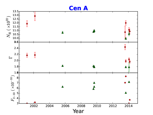
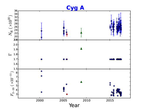
Figure 1.— The light curves of $N_{\rm H}$, $\Gamma$, and the $2-10\rm\,\,{\rm keV}$ unabsorbed flux of the sources in the sample. The red circles, blue stars and the green triangles denote the data points obtained from XMM-Newton, Chandra and Suzaku telescopes respectively.

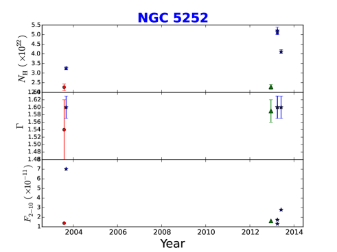
Figure 1.— The light curves of $N_{\rm H}$, $\Gamma$, and the $2-10\rm\,\,{\rm keV}$ unabsorbed flux of the sources in the sample. The red circles, blue stars and the green triangles denote the data points obtained from XMM-Newton, Chandra and Suzaku telescopes respectively.

Figure 1.— The light curves of $N_{\rm H}$, $\Gamma$, and the $2-10\rm\,\,{\rm keV}$ unabsorbed flux of the sources in the sample. The red circles, blue stars and the green triangles denote the data points obtained from XMM-Newton, Chandra and Suzaku telescopes respectively.

Figure 1.— The light curves of $N_{\rm H}$, $\Gamma$, and the $2-10\rm\,\,{\rm keV}$ unabsorbed flux of the sources in the sample. The red circles, blue stars and the green triangles denote the data points obtained from XMM-Newton, Chandra and Suzaku telescopes respectively.

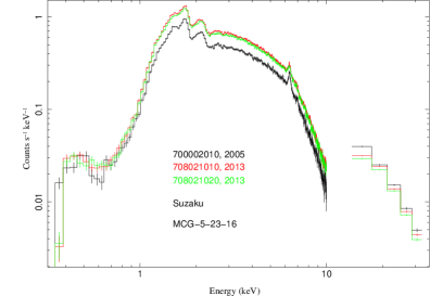
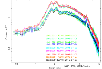
Figure 2.— The overplot of the spectra of the sources listed in Table 2 and discussed in Section 4 whose full-covering $N_{\rm H}$ values have varied between the observations. Here the spectra have been binned by a factor of four for plotting and visual purposes only. The source names, instruments, the observation identifiers (obsid), and dates of observations are written in the individual figures.

Figure 3.— Mean values of full-covering column density for each object in our sample are plotted in ranked order. Superimposed are estimates of X-ray-absorbing column density based on various optical or IR extinction, assuming the standard Galactic dust/gas conversion: Balmer decrements for broad lines or narrow lines (Maiolino et al., 2001; Malkan et al., 2017, , respectively), 9.7 $\mu$m Si line absorption (Gallimore et al., 2010), IR SED modeling (Burtscher et al., 2016), or color-color maps (Mulchaey et al., 1994a, b; Schreier et al., 1996; Prieto et al., 2014). “${\Delta}N_{\rm H}$” denotes a detection of variability in the full-covering absorption component as measured in this paper. ”PC” denotes those 11 sources wherein a partial covering component was detected in most or all of a given sources’ observations. The top row denotes the nuclear dust morphology classification from Malkan et al. (1998), for those sources included in their sample; “DC”, “D-[directional]”, “DI”, and “F/W” denote a dust lane directly crossing the line of sight to the nucleus, a dust lane just offset from the line of sight to one direction, irregular dust, and flocculent/wispy, respectively.

Figure 4.— Left panel: The histogram plots for the the $N_{\rm H}$ values of the two sets of sources in our sample, the ones which have been detected with partial covering absorption (red solid line) and the ones which do not have partial absorbers (blue dash-dotted line) Right panel: Same as left, except that here we consider the sets of sources which have shown $N_{\rm H}$ variability (pink bold line) and the ones that have not shown $N_{\rm H}$ variability (black dash-dotted line).

Appendix A Appendix A: Previous studies and details of analysis of the sources in the sample.

In this section we discuss the previous studies of the sources in the sample in context to the analysis we have carried out and science goals in the paper. We also comment on a few important issues in analysis for each of the sources and the best fit baseline model used in each case. Here NH22 denotes $N_{\rm H}/(10^{22}\rm\,\,{\rm cm^{-2}})$ :

1. CenA: This is the nearest radio-loud galaxy. RXTE monitoring revealed two previous eclipse events by transiting clouds, each causing total line-of-sight $N_{\rm H}$ to increase by $8\pm 1\times 10^{22}$ cm^-2: one in $\sim$2003–4 and one in 2010–11, studied by Rothschild et al. (2011) and Rivers et al. (2011), respectively. MKN14 inferred these clouds to reside in the inner dusty torus. As described earlier, MKN14 also noted mild, smooth variations in the baseline level of $N_{\rm H}$, thanks to the combination of Cen A’s X-ray brightness and sustained, regular monitoring (and to our knowledge, this is the only such case so far).

   Chandra data for the core of Cen A were not usable; the pileup was too severe to derive any reliable fluxes or spectral slopes (even with modeling the pileup during spectral fitting). Hence the Chandra observations were not used for this source.

   Following e.g., Markowitz et al. (2007), we model the soft band emission for the Suzaku data using two apec components plus a flat power law, the latter to model blended emission from point sources, jet components, and diffuse emission. For XMM-Newton data, using only one apec component sufficed; adding a second, lower-temperature component yielded no improvement to the fit and poor parameter constraints. No strong evidence for Compton reflection component has been found so far. Various studies with RXTE, Suzaku, INTEGRAL, and NuSTAR have yielded upper limits to the pexrav reflection fraction $R$ of e.g., 0.28, 0.05, 0.05, 0.01, and 0.005 by Beckmann et al. (2011); Markowitz et al. (2007); Benlloch et al. (2001); Fürst et al. (2016); Rivers et al. (2011), respectively; we thus freeze $R$ at 0 in our fits.

   We find evidence for a partial-covering component in observation S-1, consistent with Markowitz et al. (2007), and in X-6. We also modeled partial covering components for S-2, S-3, and S-4, following Fukazawa et al. (2011). However, for S-2, S-3, and S-4, the improvement in fit when the partial covering component is added is modest, the covering fractions are quite low, and moreover, values of $N_{\rm H,pc}$ are poorly constrained in each case, usually falling to the same value as $N_{\rm H,full}$. We detected that NH22 dropped from $11.03\pm 0.08$ (S-3) to $9.98\pm 0.14$ (S-5) and hence consider this source as a variable $N_{\rm H}$ source.

2. CygA: This is another powerful radio galaxy. Reynolds et al. (2015) observed the source with NuSTAR and measured a powerlaw $\Gamma=1.7$, a neutral absorption column of $N_{\rm H}\sim 1.6\times 10^{23}\rm\,\,{\rm cm^{-2}}$, a Compton hump at energies $>10\rm\,\,{\rm keV}$ with a reflection coefficient of $R=1.0$, and a high temperature thermal emission in the soft X-rays modeled by APEC ($kT\sim 6.4\rm\,\,{\rm keV}$).

   Here, we describe the Chandra ACIS observations of Cyg A. The active nucleus is embedded in hot, X-ray emitting gas, and Chandra ACIS has been used to image both the active nucleus and the surrounding cluster gas (e.g., Snios et al., 2018, and references therein). The archive contains dozens of observations aimed at mapping the cluster emission, with the effect that the nucleus was not observed consistently, with many observations using different ACIS-I or ACIS-S chips and having different off-axis angles to the nucleus.

   We excluded those observations where the nucleus was located in a chip gap. Backgrounds were generated using the CIAO ”blanksky” tool, as the cluster gas usually fills the majority of the ACIS chip field of view. Our model included a hard X-ray power law absorbed by a full-covering absorber; the photon index of the hard power-law was always poorly constrained, and we froze it at 1.7. We also included two APEC components and a soft power law whose photon index was also frozen at 1.7. The APEC components typically had temperatures of 0.73 and 4.0 keV.

   We paid attention to those observations where the nucleus was within 16” from the edge of a chip, as dithering could cause some fractions of photons to fall into the chip gap. However, we did not see any significant deviation in model parameters in these observations. We searched for, but did not detect, any correlation between $N_{\rm H}$ and the off-axis angle of the nucleus, or between $N_{\rm H}$ the temperature of either thermal component; there was also no correlation with the ACIS chip used.

   We find a mean value (standard deviation) in $N_{\rm H,full}$ of $(25.6\pm 2.1)\times 10^{22}\rm\,\,{\rm cm^{-2}}$. Given the variation in observations from one obsid to the next (e.g., different offset pointings, the nucleus falling on different chips), we conservatively avoid concluding that measured variations in $N_{\rm H,full}$ from one obsid to the next is intrinsic to the source, although we can rule out the presence of strong systematic trends of order $10^{24}$ cm^-2. See Table 1 for details of the best fit parameters.

   The best fit model used is tbabs*(apec+apec(2)+powerlaw(1)+ztbabs*(pexmon+powerlaw(2)+zgauss)). We do not detect significant variability in $N_{\rm H}$ for this source.

3. Fairall 49: Also known as IRAS 18325-5926. The source was studied by Iwasawa et al. (2004) who found a relatively steep powerlaw slope $\Gamma=2.2$, and a neutral absorption column of $N_{\rm H}=1.62\times 10^{22}\rm\,\,{\rm cm^{-2}}$. Kawamuro et al. (2016) detected a partial covering absorption with covering fraction of $f_{\rm PC}=0.22$ and column density of $N_{\rm H}=3.2\times 10^{22}\rm\,\,{\rm cm^{-2}}$, in addition to a full covering absorption, with Suzaku observations. We detected partial covering in addition to full covering absorption in all the observation, except for CH-2, where the low SNR did not allow us to constrain $N_{\rm H}$ of the partial absorber. We detected significant variability in $N_{\rm H}$ for this source with XMM-Newton observations, with variations of $N_{\rm H}$ by almost an order of magnitude. The best fit model used is tbabs*(apec(1)+powerlaw(1)+ztbabs*zpcfabs*(pexmon+powerlaw(2)+zgauss))

4. IRAS F00521–7054: Ricci et al. (2014) modeled the X-ray spectrum by a steep powerlaw of $\Gamma=2.2-2.3$, obscured by a neutral column of $N_{\rm H}\sim 10^{22.9}\rm\,\,{\rm cm^{-2}}$, in addition to a blurred ionised disk reflection component with a reflection coefficient of $R=2.7$. In our study, we too detected steep powerlaw slope pegged at $\Gamma=2.5$. The best fit model is tbabs*(apec+powerlaw(1)+ztbabs*zpcfabs*(pexmon+powerlaw(2)+zgauss)). We do not detect any significant variability in $N_{\rm H}$ for the source, as also concluded by a recent study by Walton et al. (2019) using NuSTAR observations.
   

5. IRAS F05189–2524: A detailed study of this source has been carried out by Teng et al. (2009), where the authors have found interesting variability in spectral shape and flux between different observations taken between 2001 and 2006 with Chandra, XMM-Newton and Suzaku satellites. The source has shown an increase in obscuring column by a factor of 10 from 2002 (Chandra) to 2006 (Suzaku) observations, although the intrinsic unabsorbed $2-10\rm\,\,{\rm keV}$ flux is constant over time. This source has been studied as a part of a sample of ULIRGs by Teng & Veilleux (2010) using Chandra observations. They found that for different observations the hard X-ray powerlaw varied from $\Gamma=1.4-2.3$ (between 2001 and 2002 observations). They also detected a non-variable partial covering absorber of the source with $N_{\rm H}\sim 7\times 10^{22}\rm\,\,{\rm cm^{-2}}$ and a covering fraction of $f^{\rm pc}\sim 0.96$. A more recent study by Teng et al. (2015) using NuSTAR data revealed a powerlaw $\Gamma=2.5$ and two partial covering absorbers of $N_{\rm H}$ of $5.2\times 10^{22}\rm\,\,{\rm cm^{-2}}$ and $9.3\times 10^{22}\rm\,\,{\rm cm^{-2}}$ with covering fractions of $98\pm 0.2\%$ and $74\pm 1.2\%$ respectively. Another study by Xu et al. (2017) using NuSTAR and XMM-Newton observations have constrained the powerlaw slope $\Gamma=2.29$ and Pexrav reflection component $R=1.48$. In our study we too required a partially covering neutral intrinsic absorber, but only for the observation X-2. The best fit model used is: tbabs*(powerlaw(1)+apec+ztbabs*zpcfabs*(zgauss+pexmon+powerlaw(1)+zgauss(2))). We do not detect any significant variability in $N_{\rm H}$ for the source.
   

6. MCG–5–23–16: Zoghbi et al. (2017) observed this source using NuSTAR for half mega seconds, with a focus on the relativistic reflection and primary coronal emission. The authors detected the presence of reflection features with a reflection coefficient of $R=0.84$. Braito et al. (2007) carried out a time resolved spectral study of this source and found that there is an absorption variability intrinsic to the source.

   In our study we found that the X-ray spectra of this source are quite complex for all the observations. In particular the high SNR long exposure XMM-Newton observations X-2, X-3 and X-4 ($\sim 130\,\rm ks$ each) exhibited several discrete spectral features which were visible after the ‘basline’ model fit. We found that in the cases of X-2, X-3 and X-4, the FeK$\alpha$ emission line and the compton reflection hump coule not be modeled simultaneously, using the pexmon parameter values obtained from Suzaku observations. We therefore thawed the pexmon normalization and this improved the fit by $\,\Delta\chi^{2}=500$. But the FeK emission line was not fully modeled, so we thawed the Fe abundance assuming that the reprocessing media for FeK emission and the Compton hump are different, which again improved the fit by $\,\Delta\chi^{2}=300$ and the best fit Fe abundance $\sim 0.15-0.19$ times solar abundance. We used a zgauss model to describe the higher ionization Fe emission lines. The best fit model used is: tbabs*(apec+powerlaw(1)+ztbabs*(pexmon+powerlaw(2)+zgauss)). We detect significant variability in $N_{\rm H}$ for the source using XMM-Newton observations.

7. Mkn 348: Marchese et al. (2014) studied this Seyfert 2 galaxy with Suzaku and XMM-Newton. The authors detected variability in the X-ray spectral curvature which they concluded could be due to changes in column density of neutral and ionized absorbers. They obtained a powerlaw photon index of $\Gamma=1.72$, a neutral absorber column density of $N_{\rm H}=4.50\times 10^{22}\rm\,\,{\rm cm^{-2}}$, and a reflection coefficient of $R=0.24_{-0.04}^{+0.04}$. In our analysis we found that the spectra need a partial covering absorber in addition to a full covering absorption, in all but one observation (CA-1, possibly due to low SNR). The best fit model used is tbabs*(apec+apec(2)+powerlaw(1)+zpcfabs*ztbabs*(zgauss+pexmon+powerlaw(1))). We detected variability in $N_{\rm H}$ between 2008 observation with Suzaku and 2010 observation with Chandra. However, the variations are within the uncertainties of cross-instrument-calibration as discussed in Section 4.2, and so we have not considered this as one of the variable $N_{\rm H}$ sources.

8. NGC 526A: This is a Seyfert 1.9 galaxy, studied by Landi et al. (2001) using BeppoSAX X-ray telescope in the energy band $0.1-150\rm\,\,{\rm keV}$. The authors detected a relatively flat powerlaw slope of $\Gamma=1.6$. Although the source flux varies strongly between the observations, the powerlaw slope remains constant over time. The reflection component detected is weak ($R\sim 0.7$). In our study we found that the best fit baseline model for this source is tbabs $\times$ (apec(1) + apec(2)+ powerlaw(1)+ ztbabs $\times$ (powerlaw(2) + pexmon + zgauss )). The spectra did not require any soft X-ray powerlaw for any of the observations. We do not detect any significant variability in $N_{\rm H}$ for the source.

9. NGC 1052: Identified as a low ionization nuclear emission region (LINER) by Heckman (1980), the galaxy hosts a low luminosity AGN (LLAGN) of a luminosity $L_{\rm 1-100GHz}=4.4\times 10^{40}\rm\,erg\,s^{-1}$ (Wrobel, 1984). The compact core of the AGN has a very flat X-ray powerlaw slope. The source is absorbed by an intrinsic neutral column of $N_{\rm H}\sim(0.6-0.8)\times 10^{22}\rm\,\,{\rm cm^{-2}}$. In our analysis we found that the Chandra observations are piled up. We used the best fit model tbabs*(apec+apec(2)+powerlaw(2)+ztbabs*zpcfabs*(zgauss+pexmon+powerlaw(1))). We detected variability in $N_{\rm H}$ between 2005 observation with Chandra and 2007 observation with Suzaku. However, due to uncertain cross-instrument-calibration we have not considered this as one of the variable $N_{\rm H}$ cases.

10. NGC 2110: Marinucci et al. (2015) studied this Seyfert 2 galaxy using NuSTAR, XMM-Newton, Chandra etc. No detectable contribution from Compton reflection has been found. The powerlaw slope $\Gamma=1.64$ and neutral absorption measured is $N_{\rm H}=4.3\times 10^{22}\rm\,\,{\rm cm^{-2}}$. In our study, the best fit model used is: tbabs $\times$ (apec(1) + powerlaw(1)+ ztbabs $\times$ zpcfabs $\times$ (powerlaw(2) + pexmon + zgauss )). For the XMM-Newton observation the frozen pexmon parameters (obtained from the Suzaku fits) were over-predicting the FeK$\alpha$ emission line, likely pointing towards a different origin of the emission line as that of the Compton hump. We thawed the Fe abundance in the pexmon fit and fitted the data. The fit improved by $\,\Delta\chi^{2}=81$, with a best fit Fe abundance of the pexmon model $\rm Fe_{\rm abund}=0.55\pm 0.07$ relative to Solar. This has also been observed in MCG-5-23-16. The powerlaw slope $\Gamma$ could not be constrained for the observation CH-2(01) and hence frozen to 1.74 (the $\Gamma$ estimated from S-1(05)). We do not detect any significant variability in $N_{\rm H}$ for the source.

11. NGC 2992: Shu et al. (2010) studied the variability of the source in X-rays. This source is known to exhibit X-ray flaring on timescales of days to weeks. They measured a powerlaw $\Gamma=1.83$, the neutral absorption column density $N_{\rm H}=6.45\times 10^{21}\rm\,\,{\rm cm^{-2}}$, the reflection fraction $R=0.40$.

    In our analysis we detected large changes in flux (almost an order of magnitude) between the XMM-Newton observation in 2003 X-1 and the rest of them in 2010 (X-2 to X-10). The X-1 observation is in an unusually high flux state of the source with both the soft and the hard X-ray bands orders of magnitude higher than the other observations. The soft X-ray band in X-1 is dominated by the nuclear emission from the AGN. In our analysis we therefore could not use averaged values for X-1. From X-1 to X-2: NH22 increased from $0.60\pm 0.01$ to $0.82\pm 0.03$ from 2003 to 2010, and hence we regard this source as a $N_{\rm H}$ variable source. The best fit model used is tbabs*(apec+powerlaw(1)+ztbabs*(zgauss+pexmon+powerlaw(2)++zgauss(3))).

12. NGC 4258: Reynolds et al. (2009) have studied this low-luminosity AGN, also classified as Seyfert-2, with XMM-Newton and Suzaku. The authors conclude that the circumnuclear environment of this AGN is very clean and lacks Compton-thick obscuring torus. They obtained a best fit powerlaw $\Gamma=1.75$, and an absorption column of $N_{\rm H}=9.2\times 10^{22}\rm\,\,{\rm cm^{-2}}$. In our analysis we found that this source has spatially extended structures in soft X-ray emission as viewed with XMM EPIC-pn camera. The best fit model we used is tbabs*(apec+apec(2)+powerlaw(1)+ztbabs*(zgauss+pexmon+powerlaw(2))). We do not detect any significant variability in $N_{\rm H}$ for the source.

13. NGC 4507: The Chandra HETG and XMM-Newton data of this source has been studied by Matt et al. (2004) where they detect a Compton-thin absorption of column density of $N_{\rm H}=4\times 10^{23}\rm\,\,{\rm cm^{-2}}$. This source has also been studied as a part of a sample using Suzaku data by Kawamuro et al. (2016), and the authors found that the source required a Compton-thin absorber, a partial covering absorber and a neutral reflection component of $R=0.43\pm 0.07$. The powerlaw slope estimated by the authors are $\Gamma=1.79$. In our study, the best fit model used is tbabs*(apec+apec(2)+powerlaw(1)+zgauss(2)+ztbabs*zpcfabs*(zgauss+pexmon+powerlaw(2))). We do not detect any significant variability in $N_{\rm H}$ for the source.

14. NGC 5252: Dadina et al. (2010) studied this source with Chandra. The intrinsic powerlaw slope and absorption column density obtained are $\Gamma=1.4-1.5$, and $N_{\rm H}=10^{22}\rm\,\,{\rm cm^{-2}}$ respectively. No mention is made of a possible Compton hump.

    In our fits to the Chandra-ACIS data, $\Gamma_{\rm Hard}$ is very poorly constrained, but we obtained best fits when it is frozen at 1.4 (i.e., forcing $\Gamma_{\rm Hard}$ to 1.66, as measured by Kawamuro et al. (2016) with Suzaku, yielded high values of $\chi^{2}_{\nu}\sim 1.2$). This value consistent with previous fits to Chandra data done by Dadina et al. (2010), who measured $\Gamma=1.4-1.5$. Traditionally, such flat values of $\Gamma_{\rm Hard}$ culd be attributed to unmodeled Compton Reflection Hump emission, but we did not find any mention in the literature of a Compton Hump, and our fits to the Suzaku data did not require one.

    In our study, the best fit model used is tbabs*(apec+apec(2)+powerlaw(1)+zpcfabs*ztbabs*(zgauss+pexmon+powerlaw(2))). We obtained good fits in the soft band by using a single apec component with a common temperature and normalization for all four spectra. $\Gamma_{\rm Soft}$ was poorly constrained, but an average value of 1.32 allowed for good fits in all four spectra. However, the soft power-law normalization was found to vary: Satisfactory fits to CA2, CA3, and CA4 were obtained with an average normalization of $9.65\times 10^{-5}$, but for CA1, which occurred ten years earlier, this value yielded a poor fit. CA1 required a normalization of $4.50\pm 0.43\times 10^{-5}$ (and in the MultiNest runs, this parameter is left free in CA1).

    Partial coverers were required in the XMM-Newton and Suzaku data only. We tried to insert partial coverers into the Chandra fits, but could obtain reasonable constraints on those parameters. We note, though, that through using various values of photon index or requiring/lacking partial coverers, that the sequence of $N_{\rm H}$ values in the ACIS data always consistently followed $N_{\rm H}$(CA1) $<$ $N_{\rm H}$(CA2) $\sim$ $N_{\rm H}$(CA3) $>$ $N_{\rm H}$(CA4), and $N_{\rm H}$(CA1) $<$ $N_{\rm H}$(CA4).

15. NGC 5506: Matt et al. (2015) studied this source using NuSTAR observations. They found that the spectrum is well fitted by $\Gamma=1.9$ intrinsically absorbed by $N_{\rm H}=3.10\times 10^{22}\rm\,\,{\rm cm^{-2}}$, and a distant reflection component and narrow Fe emission lines. Guainazzi et al. (2010) studied this source using XMM-Newton and measured a $\Gamma=1.9$.

    In our study, we used the best fit model tbabs*(ztbabs(2)*(apec+powerlaw(1))+zgauss(3)+ztbabs*(pexmon+powerlaw(1)+
    zgauss+zgauss(2))). Note that we required two different full covering absorbers. One that absorbs the central AGN and the other which absorbs both the AGN and the outer parts of the galaxy (stellar emission) with a lower absorbing column density. The outer absorption column density is $N_{\rm H}\sim 10^{20}\rm\,\,{\rm cm^{-2}}$, and the inner absorption column $N_{\rm H}\sim 10^{22}\rm\,\,{\rm cm^{-2}}$ . Most of the Chandra observations are piled-up and the pile-up could not be modeled using the pile-up kernel alone, hence we have reported only one Chandra-HETG observation which has lower pile-up. We detect significant variability of $N_{\rm H}$ in this source, with a gradual increase in column density from 2002-2004. The XMM-Newton observation of this source X9, has a long exposure ($\sim 132\,\rm ks$) with high SNR. The soft X-ray spectra ($<1.3\rm\,\,{\rm keV}$) could be modeled by a single Apec model component with a higher normalization but a lower abundance of elements, $Z=0.0162\pm 0.0012$ relative to Solar, as also detected in previous studies (Bianchi et al., 2003). We did not require any soft X-ray powerlaw for this observation. The measured value of $N_{\rm H}=(3.00\pm 0.01)\times 10^{22}\rm\,\,{\rm cm^{-2}}$ for this observation is consistent with those detected for observations from 2004-2015 indicating a constant absorption for that period of time.

16. NGC 6251: This is a low excitation radio loud galaxy. Evans et al. (2011) studied the Suzaku observation and detected a powerlaw of $\Gamma=1.82$ and two thermal plasma components, $kT=0.89\rm\,\,{\rm keV}$, and $kT=2.63\rm\,\,{\rm keV}$, and no reflection component in the hard X-rays. The authors however could not rule out a Compton-thick obscuration. In our analysis the best fit model used is tbabs*(apec+powerlaw(1)+ztbabs*(pexmon+powerlaw(2)+zgauss)). The Chandra-ACIS observation has no sufficient SNR to constrain the column density. We do not detect any significant variability in $N_{\rm H}$ for the source.

17. NGC 6300: Matsumoto et al. (2004) studied the Seyfert 2 galaxy using XMM-Newton and obtained a powerlaw $\Gamma=1.83\pm 0.08$ and a Compton-thin absorber of column density $N_{\rm H}=2.2\times 10^{23}\rm\,\,{\rm cm^{-2}}$. The authors could model the soft emission using a powerlaw. The relative reflection strength producing the Compton hump is estimated to be $R=1.1_{-0.6}^{+1.1}$ using Pexrav model. In our study we used the best fit model: tbabs*(apec+powerlaw(1)+ztbabs*(zgauss+pexmon+powerlaw(2))). We do not detect any significant variability in $N_{\rm H}$ for the source.

18. NGC 7172: Awaki et al. (2006) studied the variability of this source in a sample of Seyfert 2 galaxies, and measured a $\Gamma=1.55\pm 0.07$, and an absorption column of $N_{\rm H}=(8.3\pm 0.4)\times 10^{22}\rm\,\,{\rm cm^{-2}}$. Akylas et al. (2001) have studied this source and detected a flatter slope of $\Gamma=1.64$ and a neutral absorption of $N_{\rm H}=9.0\times 10^{22}\rm\,\,{\rm cm^{-2}}$. However, they could not rule out the possiblity of an alternative scenario of a steeper slope of $\Gamma=1.78$ and a reflection component of $R=1.2_{-0.9}^{+0.7}$. In our work we found that the Chandra observations are mostly piled up. The best fit model we have used is tbabs*(powerlaw(1) + apec(2) + ztbabs * zpcfabs * (zgauss+pexmon+powerlaw(2))). We do not detect any significant variability in $N_{\rm H}$ for the source.

19. NGC7314: Ebrero et al. (2011) studied the source using XMM-Newton and Suzaku and found that the source shows rapid short term variability. No Compton reflection was detected. A powerlaw slope of $\Gamma=2.14$ was measured along with a neutral absorber column of $N_{\rm H}=2.9\times 10^{21}\rm\,\,{\rm cm^{-2}}$. Dewangan & Griffiths (2005) studied this source as a part of a small sample of obscured NLSy1 galaxies and found a reflection component of $R=2.83$, $\Gamma=2.19$, and no intrinsic absorption.In our study, we used the best fit model tbabs*(apec+powerlaw+ztbabs*(zgauss+pexrav)). We do not detect any significant variability in $N_{\rm H}$ for the source.

20. NGC 7582: This is a star-burst dominated galaxy with a Seyfert 2 nucleus at the centre. Rivers et al. (2015) studied the source using NuSTAR and found that the source is variable with strong reflection features. The obscuring torus is patchy with a covering fraction of $80-90\%$ with a column density of $3.6\times 10^{24}\rm\,\,{\rm cm^{-2}}$. Another full covering absorber was also needed with a column density of $\sim 3-12\times 10^{23}\rm\,\,{\rm cm^{-2}}$. The authors modeled the Compton hump with a Pexrav model with a best fit reflection $R=4.3$, which is much higher than expected. The authors suggest that the geometry of the reflecting material is not that of a flat disk. The powerlaw photon index obtained by them is $\Gamma=1.78\pm 0.07$. Bianchi et al. (2009) studied this source with Suzaku. The source is characterized by very rapid changes of the column density of an inner absorber, which makes the authors conclude the presence of complex absorbing system and not just a simple torus followed from the unification model.

    In our study the best fit model used is tbabs*(apec + apec(2) + apec(3) + powerlaw + zpcfabs * ztbabs * (zgauss + pexrav + zgauss(2) + zgauss(3) + zgauss(4))) . We detected variability of $N_{\rm H}$ in this source both using XMM-Newton and Suzaku observations. However, the Suzaku estimated values of $N_{\rm H}$ are different with respect to each other at only 90% error margins obtained using ISIS, and do not qualify our ‘variability’ criteria described in Section 4.1. Due to high SNR in the XMM-Newton observations, we detected discrete emission lines at $2.5\rm\,\,{\rm keV}$ (Sulphur K-$\alpha$) and $6.4\rm\,\,{\rm keV}$, $7.12\rm\,\,{\rm keV}$ and $7.5\rm\,\,{\rm keV}$ indicative of FeK$\alpha$ and higher ionization of Fe emission lines. The observations X-1 and X-2 required a partial covering absorption, while X-3 and X-4 did not require them. When we used a zpcfabs model for X-3 and X-4 and froze the parameter values to those obtained in X-1, we found that fit worsened by $\,\Delta\chi^{2}=200$. When left free the value of $N_{\rm H}^{\rm pc}$ went to zero with an improvement in statistics. We required three Apec models for this source, possibly because this source is dominated by stellar emission from different regions in the galaxy (with different temperatures and emissivity) in the soft X-rays.

Appendix B Appendix B: CygA Chandra observations

In this section we list the best fit parameters obtained from the fits to the Chandra observation of Cyg A (See Table 1).

Table 1The Chandra observations of Cyg-A and the best fit absorption column densities, Apec temperatures and best fit statistic. The powerlaw slope has been fixed at $\Gamma=1.7$ in all cases.

Chandra obs-id	Date of obs	$N_{\rm H}$	Apec-KT	Apec-KT	Fluxesa	$\chi^{2}/\chi^{2}_{\nu}$
		$(\times 10^{22}\rm\,\,{\rm cm^{-2}})$	($\rm\,\,{\rm keV}$)	($\rm\,\,{\rm keV}$)	$\times 10^{-11}\rm\,erg\,cm^{-2}\,s^{-1}$
359	2000-03-08	$23.6^{+5.0}_{-4.1}$	1.1	4.6	8.40	$25.93/0.960$
360	2000-05-21	$23.6^{+1.5}_{-1.4}$	0.26	1.9	3.52	$375.92/0.989$
1707	2000-05-26	$19.6^{+1.6}_{-1.4}$	0.28	2.0	7.28	$170.69/0.938$
6225	2005-02-15	$21.9^{+1.5}_{-1.8}$	0.92	3.9	3.77	$298.73/1.205$
5831	2005-02-16	$22.6^{+1.2}_{-1.1}$	0.78	3.3	4.22	$448.74/1.039$
6226	2005-02-19	$23.7^{+1.8}_{-1.6}$	1.1	3.5	4.23	$270.43/1.104$
6250	2005-02-21	$25.4^{+4.3}_{-3.5}$	0.43	3.3	4.57	$80.97/0.976$
5830	2005-02-22	$25.9^{+2.1}_{-2.0}$	0.43	4.0	4.14	$265.78/1.089$
6229	2005-02-23	$25.3^{+1.8}_{-1.8}$	0.69	4.1	4.26	$228.11/0.939$
6228	2005-02-25	$23.5^{+2.1}_{-2.0}$	0.85	2.7	4.50	$156.82/0.866$
6252	2005-09-07	$22.8^{+1.6}_{-1.5}$	0.93	4.0	5.33	$350.30/1.052$
17505	2015-01-05	$26.4^{+1.0}_{-0.8}$	0.82	4.9	5.21	$471.77/1.051$
17145	2015-01-10	$25.6^{+1.0}_{-0.9}$	0.97	5.1	5.66	$420.56/0.960$
17530	2015-04-19	$24.2^{+3.1}_{-2.6}$	0.52	4.7	2.85	$116.75/0.965$
17650	2015-04-22	$29.7^{+3.8}_{-2.9}$	1.06	7.0	2.75	$161.40/1.121$
17144	2015-05-03	$28.1^{+2.1}_{-1.9}$	0.74	4.7	3.52	$236.37/0.879$
17528	2015-08-30	$26.1^{+1.5}_{-1.4}$	0.88	3.7	3.37	$390.46/1.004$
17143	2015-09-03	$23.1^{+1.8}_{-1.7}$	0.68	2.7	3.32	$228.42/1.053$
17524	2015-09-08	$26.9^{+2.4}_{-2.2}$	0.66	2.6	2.87	$196.28/1.175$
18441	2015-09-14	$26.3^{+2.2}_{-2.2}$	0.86	3.5	2.82	$186.22/1.029$
17526	2015-09-20	$25.4^{+1.1}_{-1.3}$	0.35	3.3	3.34	$397.67/1.063$
17527	2015-10-11	$26.3^{+2.3}_{-2.3}$	0.92	4.5	3.74	$159.48/0.886$
18682	2015-10-14	$24.4^{+3.3}_{-2.3}$	0.79	7.2	3.32	$142.93/0.928$
18641	2015-10-15	$26.0^{+2.8}_{-2.7}$	2.0	4.0	3.16	$121.57/0.921$
18683	2015-10-18	$24.2^{+3.8}_{-2.7}$	0.69	4.3	2.67	$98.54/1.263$
17508	2015-10-28	$27.7^{+2.9}_{-2.6}$	1.0	4.4	4.06	$144.79/0.894$
18688	2015-11-01	$27.8^{+1.7}_{-1.6}$	0.54	1.3	4.96	$344.60/0.999$
18871	2016-06-13	$29.1^{+2.4}_{-2.5}$	0.44	2.7	3.92	$200.73/0.947$
17133	2016-06-18	$25.3^{+2.1}_{-1.9}$	0.85	3.5	3.39	$298.38/1.033$
17510	2016-06-26	$26.2^{+1.7}_{-1.6}$	1.03	4.4	3.91	$311.58/0.898$
17509	2016-07-10	$24.5^{+1.3}_{-1.2}$	0.70	3.6	3.74	$414.29/0.989$
17518	2016-07-16	$23.2^{+1.2}_{-1.4}$	0.52	4.0	3.62	$382.97/0.930$
17521	2016-07-20	$23.2^{+1.9}_{-1.8}$	0.43	2.0	3.78	$297.22/1.126$
18886	2016-07-23	$24.7^{+1.9}_{-1.8}$	0.69	2.6	4.20	$234.27/1.014$
17138	2016-07-25	$22.6^{+1.5}_{-1.6}$	0.89	2.9	3.97	$320.98/1.180$
17513	2016-08-15	$26.2^{+1.4}_{-1.4}$	0.76	4.0	4.20	$428.77/1.033$
17516	2016-08-18	$24.3^{+1.4}_{-1.3}$	0.67	3.2	3.82	$418.26/1.023$
17523	2016-08-31	$23.5^{+1.7}_{-1.6}$	1.04	4.8	2.67	$258.93/0.838$
17512	2016-09-15	$24.9^{+1.2}_{-1.2}$	0.82	3.8	3.73	$445.67/0.975$
17139	2016-09-16	$27.3^{+1.9}_{-1.7}$	0.54	2.2	4.00	$361.65/1.005$
17517	2016-09-17	$25.2^{+2.0}_{-1.9}$	1.11	4.1	3.65	$253.62/0.998$
19888	2016-10-01	$25.4^{+2.1}_{-1.9}$	0.43	5.5	4.17	$194.71/0.969$
17140	2016-10-02	$27.4^{+2.0}_{-1.8}$	0.44	2.2	4.22	$304.83/0.929$
17507	2016-11-12	$25.6^{+1.9}_{-1.7}$	1.06	4.3	3.49	$319.56/1.055$
17520	2016-12-06	$31.0^{+3.0}_{-2.6}$	0.74	10.9	3.58	$209.14/0.890$
19956	2016-12-10	$26.4^{+1.6}_{-1.4}$	0.71	5.0	3.47	$391.13/0.959$
17514	2016-12-13	$24.1^{+1.4}_{-1.3}$	0.72	2.8	3.54	$407.98/0.990$
17529	2016-12 15	$25.1^{+1.8}_{-1.7}$	0.98	1.7	3.86	$314.61/0.948$
17519	2016-12-19	$28.2^{+2.3}_{-2.0}$	0.17	4.3	3.86	$7300.66/1.051$
17135	2017-01-20	$29.1^{+2.6}_{-2.4}$	0.70	3.8	4.15	$182.04/0.910$
17136	2017-01-26	$26.0^{+2.3}_{-2.0}$	0.12	3.2	3.58	$216.93/1.028$
19996	2017-01-28	$26.3^{+2.0}_{-1.8}$	0.54	4.4	3.32	$282.59/1.075$

^a The $2-10\rm\,\,{\rm keV}$ unasborbed power law fluxes.

Table 1The Chandra observations of Cyg-A and the best fit absorption column densities, Apec temperatures and best fit statistic. The powerlaw slope has been fixed at $\Gamma=1.7$ in all cases.

Chandra obs-id	Date of obs	$N_{\rm H}$	Apec-KT	Apec-KT	Fluxes	$\chi^{2}/\chi^{2}_{\nu}$
		$(\times 10^{22}\rm\,\,{\rm cm^{-2}})$	($\rm\,\,{\rm keV}$)	($\rm\,\,{\rm keV}$)	$\times 10^{-11}\rm\,erg\,cm^{-2}\,s^{-1}$
19989	2017-02-12	$26.5^{+1.6}_{-1.6}$	0.68	3.9	3.48	373.15/1.014
17515	2017-03-21	$24.9^{+1.7}_{-1.5}$	0.7	4.2	3.23	295.30/0.937
20043	2017-03-25	$27.7^{+2.3}_{-2.1}$	1.0	6.9	3.14	194.67/0.801
20044	2017-03-26	$22.6^{+2.3}_{-2.1}$	0.12	2.4	3.47	140.45/1.025
17137	2017-03-29	$26.1^{+2.0}_{-2.0}$	1.4	5.0	3.20	215.37/1.002
17522	2017-04-08	$27.5^{+1.6}_{-1.5}$	0.72	5.9	3.49	336.64/0.879
20059	2017-04-19	$30.0^{+4.8}_{-2.7}$	0.27	4.3	2.95	114.31/1.099
17142	2017-04-20	$27.0^{+3.4}_{-2.7}$	0.54	5.0	2.88	174.94/1.346
17525	2017-04-22	$24.4^{+1.8}_{-2.3}$	1.22	4.1	2.62	191.00/1.151
20063	2017-04-22	$28.1^{+3.7}_{-2.6}$	0.88	6.3	3.18	193.57/1.030
17511	2017-05-10	$24.3^{+2.8}_{-2.2}$	0.44	2.4	3.46	131.70/0.808
20077	2017-05-13	$24.6^{+2.}_{-1.9}$	0.21	4.2	3.25	272.28/1.072
20048	2017-05-19	$26.9^{+3.2}_{-2.7}$	0.70	3.5	2.78	119.64/0.989
17134	2017-05-20	$25.1^{+1.8}_{-1.7}$	1.1	4.3	3.46	270.15/0.986
20079	2017-05-21	$25.8^{+2.8}_{-2.3}$	0.74	2.8	3.13	229.10/1.046

Appendix C Appendix C: The spectral overplots

Figure 1.— The overplot of the spectra of Cen A. Here the spectra have been binned by a factor of four for plotting and visual purposes only.

Figure 2.— Same as Fig. 1, except for the source which is Cyg A.

Figure 3.— Same as Fig. 1, except for the source which is Fairall 49

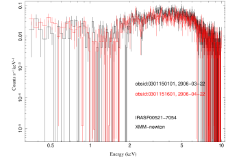
Figure 4.— Same as Fig. 1, except for the source which is IRASF00521.

Figure 5.— Same as Fig. 1, except for the source which is IRASF05189

Figure 6.— Same as Fig. 1, except for the source which is MCG-5-23-16.

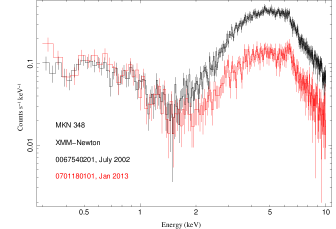
Figure 7.— Same as Fig. 1, except for the source which is MKN 348.

Figure 8.— Same as Fig. 1, except for the source which is NGC 526A

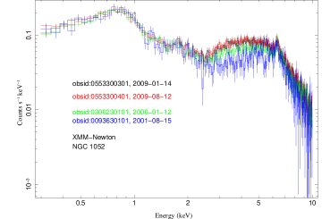
Figure 9.— Same as Fig. 1, except for the source which is NGC 1052.

Figure 10.— Same as Fig. 1, except for the source which is NGC 2110.

Figure 11.— Same as Fig. 1, except for the source which is NGC 2992.

Figure 12.— Same as Fig. 1, except for the source which is NGC 4258

Figure 13.— Same as Fig. 1, except for the source which is NGC 4507

Figure 14.— Same as Fig. 1, except for the source which is NGC 5252

Figure 15.— Same as Fig. 1, except for the source which is NGC 5506

Figure 16.— Same as Fig. 1, except for the source which is NGC 6251

Figure 17.— Same as Fig. 1, except for the source which is NGC 6300

Figure 18.— Same as Fig. 1, except for the source which is NGC 7172

Figure 19.— Same as Fig. 1, except for the source which is NGC 7314.

Figure 20.— Same as Fig. 1, except for the source which is NGC 7582.

Appendix D Appendix D: Bayesian X-ray Analysis (BXA) simulations

As discussed in Section 4, we ran the MultiNest nested-sampling algorithm (Skilling 2004; Feroz et al. 2009) via the Bayesian X-ray Analysis (BXA) and PyMultiNest packages (Buchner et al. 2014) for XSPEC version 12.10.1f to assess fit parameter distributions and explore potential model degeneracies between $N_{\rm H}$ and other model parameters. Due to the long computational times required, it was not feasible to run MultiNest on all observations for a given source/instrument combination. Instead we ran MultiNest on select cases of interest to make sure that deviating parameter values for a particular observation were not the result of e.g., a low exposure time in that observation (as we had initially suspected, but then ruled out, for Cen A S5).

We caution the reader, however, about the limitations of such simulations, as they are intended for exploring fit parameter distributions for an assumed model. They are not intended for determining goodness-of-fit of that model to the observed data. In addition, a couple assumptions implicit in these simulations are worth noting. When we specify a model as input for these simulations, we implicitly assume that the input model is accurate in terms of containing the proper components (we assume we’re not missing spectral components that are intrinsically present in the source, nor have we added components to our model that are intrinsically lacking in the source). We also assume that each spectral component intrinsically present in the real data follows the equation-based model components we use (e.g., we assume that the real data’s primary continuum indeed follows a strict power law). If the real data has, for example, some very mild continuum curvature such that our modeling cannot signficantly reject a strict power law, then best-fit parameters could differ slightly between in the observed/modeled spectrum and the simulated spectra.

We display the resulting parameter posterior contour plots in Figures 1 through 12.

Figure 1.— Parameter posterior distributions for the MultiNest run of Cen A, observation S-5. Green solid lines denote the median posterior value; dashed black lines denote the 5 and 95$\%$-tile values. The solid black contours denote the 68, 90, and 99$\%$ confidence levels. Here, $A_{\rm apec1,2}$ denote apec normalizations, $A_{\rm S,H}$ denote the 1 keV normalization of the soft- and hard-band power laws, $A_{\rm HXD}$ refers to the HXD-PIN/XIS0 cross-instrument constant.

Figure 2.— Same as Fig. 1, but for Fairall49, X1. Here, $N_{\rm H,pc}$ and $f_{\rm pc}$ denote partial-covering absorber parameters.

Figure 3.— Same as Fig. 1, but for Fairall 49, X2

Figure 4.— Same as Fig. 1, but for MCG-5-23-16, S-1

Figure 5.— Same as Fig. 1, but for MCG-5-23-16, X1

Figure 6.— Same as Fig. 1, but for NGC 2992, X1

Figure 7.— Same as Fig. 1, but for NGC 5252, CA-1

Figure 8.— Same as Fig. 1, but for NGC 5252, CA4

Figure 9.— Same as Fig. 1, but for NGC 5506, X1. Here, $N_{\rm H,1}$ refers to the component absorbing the soft-band emission components, as discussed in Appendix A; $N_{\rm H,2}$ refers to the variable full-covering absorber absorbing the hard-band components.

Figure 10.— Same as Fig. 9, but for NGC 5506 X3.

Figure 11.— Same as Fig. 1, but for NGC 7582, X1

Figure 12.— Same as Fig. 1, but for NGC 7582 X-4, and which lacks a partial-covering component.

References

- Akylas et al. (2001) Akylas, A., Georgantopoulos, I., & Comastri, A. 2001, MNRAS, 324, 521
- Antonucci & Miller (1985) Antonucci, R. R. J., & Miller, J. S. 1985, ApJ, 297, 621
- Awaki et al. (2006) Awaki, H., Murakami, H., Ogawa, Y., & Leighly, K. M. 2006, ApJ, 645, 928
- Awaki et al. (2008) Awaki, H., et al. 2008, PASJ, 60, S293
- Baskin & Laor (2018) Baskin, A., & Laor, A. 2018, MNRAS, 474, 1970
- Bassani et al. (1999) Bassani, L., Dadina, M., Maiolino, R., Salvati, M., Risaliti, G., Della Ceca, R., Matt, G., & Zamorani, G. 1999, ApJS, 121, 473
- Beckmann et al. (2011) Beckmann, V., Jean, P., Lubiński, P., Soldi, S., & Terrier, R. 2011, A&A, 531, A70
- Benlloch et al. (2001) Benlloch, S., Rothschild, R. E., Wilms, J., Reynolds, C. S., Heindl, W. A., & Staubert, R. 2001, A&A, 371, 858
- Bianchi et al. (2003) Bianchi, S., Balestra, I., Matt, G., Guainazzi, M., & Perola, G. C. 2003, A&A, 402, 141
- Bianchi et al. (2007) Bianchi, S., Chiaberge, M., Piconcelli, E., & Guainazzi, M. 2007, MNRAS, 374, 697
- Bianchi et al. (2006) Bianchi, S., Guainazzi, M., & Chiaberge, M. 2006, A&A, 448, 499
- Bianchi et al. (2012a) Bianchi, S., Maiolino, R., & Risaliti, G. 2012a, Advances in Astronomy, 2012, 782030
- Bianchi et al. (2009) Bianchi, S., Piconcelli, E., Chiaberge, M., Bailón, E. J., Matt, G., & Fiore, F. 2009, ApJ, 695, 781
- Bianchi et al. (2012b) Bianchi, S., et al. 2012b, MNRAS, 426, 3225
- Blandford & Payne (1982) Blandford, R. D., & Payne, D. G. 1982, MNRAS, 199, 883
- Blustin et al. (2005) Blustin, A. J., Page, M. J., Fuerst, S. V., Brand uardi-Raymont, G., & Ashton, C. E. 2005, A&A, 431, 111
- Boone et al. (2011) Boone, F., et al. 2011, A&A, 525, A18
- Braito et al. (2007) Braito, V., et al. 2007, ApJ, 670, 978
- Buchner & Bauer (2017) Buchner, J., & Bauer, F. E. 2017, MNRAS, 465, 4348
- Buchner et al. (2014) Buchner, J., et al. 2014, A&A, 564, A125
- Burtscher et al. (2016) Burtscher, L., Davies, R. I., Graciá-Carpio, J., Koss, M. J., Lin, M.-Y., Lutz, D., & Nandra, P. a. 2016, A&A, 586, A28
- Cappellari et al. (2009) Cappellari, M., Neumayer, N., Reunanen, J., van der Werf, P. P., de Zeeuw, P. T., & Rix, H. W. 2009, MNRAS, 394, 660
- Cappi et al. (2006) Cappi, M., et al. 2006, A&A, 446, 459
- Combes et al. (2019) Combes, F., et al. 2019, A&A, 623, A79
- Contopoulos & Lovelace (1994) Contopoulos, J., & Lovelace, R. V. E. 1994, ApJ, 429, 139
- Czerny & Hryniewicz (2011) Czerny, B., & Hryniewicz, K. 2011, A&A, 525, L8
- Dadina et al. (2010) Dadina, M., Guainazzi, M., Cappi, M., Bianchi, S., Vignali, C., Malaguti, G., & Comastri, A. 2010, A&A, 516, A9
- Dewangan & Griffiths (2005) Dewangan, G. C., & Griffiths, R. E. 2005, ApJ, 625, L31
- Dorodnitsyn & Kallman (2012) Dorodnitsyn, A., & Kallman, T. 2012, ApJ, 761, 70
- Driver et al. (2007) Driver, S. P., Popescu, C. C., Tuffs, R. J., Liske, J., Graham, A. W., Allen, P. D., & de Propris, R. 2007, MNRAS, 379, 1022
- Ebrero et al. (2011) Ebrero, J., Costantini, E., Kaastra, J. S., de Marco, B., & Dadina, M. 2011, A&A, 535, A62
- Elitzur (2007) Elitzur, M. 2007, in Astronomical Society of the Pacific Conference Series, Vol. 373, The Central Engine of Active Galactic Nuclei, ed. L. C. Ho & J. W. Wang, 415
- Elitzur & Ho (2009) Elitzur, M., & Ho, L. C. 2009, ApJ, 701, L91
- Elitzur & Shlosman (2006) Elitzur, M., & Shlosman, I. 2006, ApJ, 648, L101
- Evans et al. (2011) Evans, D. A., Summers, A. C., Hardcastle, M. J., Kraft, R. P., Gandhi, P., Croston, J. H., & Lee, J. C. 2011, ApJ, 741, L4
- Feroz et al. (2009) Feroz, F., Hobson, M. P., & Bridges, M. 2009, MNRAS, 398, 1601
- Ferrarese & Ford (1999) Ferrarese, L., & Ford, H. C. 1999, ApJ, 515, 583
- Fukazawa et al. (2011) Fukazawa, Y., et al. 2011, ApJ, 743, 124
- Fukumura et al. (2010) Fukumura, K., Kazanas, D., Contopoulos, I., & Behar, E. 2010, ApJ, 715, 636
- Fürst et al. (2016) Fürst, F., et al. 2016, ApJ, 819, 150
- Gallimore et al. (2010) Gallimore, J. F., et al. 2010, ApJS, 187, 172
- Gallimore et al. (2016) —. 2016, ApJ, 829, L7
- García-Burillo et al. (2016) García-Burillo, S., et al. 2016, ApJ, 823, L12
- Goulding et al. (2012) Goulding, A. D., Alexander, D. M., Bauer, F. E., Forman, W. R., Hickox, R. C., Jones, C., Mullaney, J. R., & Trichas, M. 2012, ApJ, 755, 5
- Guainazzi & Bianchi (2007) Guainazzi, M., & Bianchi, S. 2007, MNRAS, 374, 1290
- Guainazzi et al. (2010) Guainazzi, M., Bianchi, S., Matt, G., Dadina, M., Kaastra, J., Malzac, J., & Risaliti, G. 2010, MNRAS, 406, 2013
- Guainazzi et al. (2001) Guainazzi, M., Fiore, F., Matt, G., & Perola, G. C. 2001, MNRAS, 327, 323
- Guainazzi et al. (2005) Guainazzi, M., Matt, G., & Perola, G. C. 2005, A&A, 444, 119
- Heckman (1980) Heckman, T. M. 1980, A&A, 87, 152
- Herrnstein et al. (1999) Herrnstein, J. R., et al. 1999, Nat, 400, 539
- Hönig et al. (2013) Hönig, S. F., et al. 2013, ApJ, 771, 87
- Houck & Denicola (2000) Houck, J. C., & Denicola, L. A. 2000, in Astronomical Society of the Pacific Conference Series, Vol. 216, Astronomical Data Analysis Software and Systems IX, ed. N. Manset, C. Veillet, & D. Crabtree, 591
- Imanishi et al. (2016) Imanishi, M., Nakanishi, K., & Izumi, T. 2016, ApJ, 822, L10
- Imanishi et al. (2018) Imanishi, M., Nakanishi, K., Izumi, T., & Wada, K. 2018, ApJ, 853, L25
- Iwasawa et al. (2004) Iwasawa, K., Lee, J. C., Young, A. J., Reynolds, C. S., & Fabian, A. C. 2004, MNRAS, 347, 411
- Jaffe et al. (2004) Jaffe, W., et al. 2004, Nat, 429, 47
- Kalberla et al. (2005) Kalberla, P. M. W., Burton, W. B., Hartmann, D., Arnal, E. M., Bajaja, E., Morras, R., & Pöppel, W. G. L. 2005, A&A, 440, 775
- Kallman & Bautista (2001) Kallman, T., & Bautista, M. 2001, ApJS, 133, 221
- Kawamuro et al. (2016) Kawamuro, T., Ueda, Y., Tazaki, F., Ricci, C., & Terashima, Y. 2016, ApJS, 225, 14
- Kishimoto et al. (2009) Kishimoto, M., Hönig, S. F., Antonucci, R., Kotani, T., Barvainis, R., Tristram, K. R. W., & Weigelt, G. 2009, A&A, 507, L57
- Konigl & Kartje (1994) Konigl, A., & Kartje, J. F. 1994, ApJ, 434, 446
- Koyama et al. (2007) Koyama, K., Tsunemi, H., Dotani, T., & Bautz, M. W. 2007, PASJ, 59, 23
- Kraft et al. (2008) Kraft, R. P., et al. 2008, ApJ, 677, L97
- Krolik & Begelman (1988) Krolik, J. H., & Begelman, M. C. 1988, ApJ, 329, 702
- Lagos et al. (2011) Lagos, C. D. P., Padilla, N. D., Strauss, M. A., Cora, S. A., & Hao, L. 2011, MNRAS, 414, 2148
- Laha et al. (2014) Laha, S., Guainazzi, M., Dewangan, G. C., Chakravorty, S., & Kembhavi, A. K. 2014, MNRAS, 441, 2613
- Lamer et al. (2003) Lamer, G., Uttley, P., & McHardy, I. M. 2003, MNRAS, 342, L41
- Landi et al. (2001) Landi, R., et al. 2001, A&A, 379, 46
- Maiolino et al. (2001) Maiolino, R., Marconi, A., & Oliva, E. 2001, A&A, 365, 37
- Maiolino & Rieke (1995) Maiolino, R., & Rieke, G. H. 1995, ApJ, 454, 95
- Maiolino et al. (2010) Maiolino, R., et al. 2010, A&A, 517, A47
- Malkan et al. (1998) Malkan, M. A., Gorjian, V., & Tam, R. 1998, ApJS, 117, 25
- Malkan et al. (2017) Malkan, M. A., Jensen, L. D., Rodriguez, D. R., Spinoglio, L., & Rush, B. 2017, ApJ, 846, 102
- Marchese et al. (2014) Marchese, E., et al. 2014, MNRAS, 437, 2806
- Marinucci et al. (2015) Marinucci, A., Matt, G., Bianchi, S., Lu, T. N., & Arevalo, P. 2015, MNRAS, 447, 160
- Markowitz et al. (2007) Markowitz, A., Takahashi, T., Watanabe, S., Nakazawa, K., & Fukazawa, Y. 2007, ApJ, 665, 209
- Markowitz et al. (2014) Markowitz, A. G., Krumpe, M., & Nikutta, R. 2014, MNRAS, 439, 1403
- Matsumoto et al. (2004) Matsumoto, C., Nava, A., Maddox, L. A., Leighly, K. M., Grupe, D., Awaki, H., & Ueno, S. 2004, ApJ, 617, 930
- Matt (2000) Matt, G. 2000, A&A, 355, L31
- Matt et al. (2004) Matt, G., Bianchi, S., D’Ammando, F., & Martocchia, A. 2004, A&A, 421, 473
- Matt et al. (2015) Matt, G., et al. 2015, MNRAS, 447, 3029
- Moran et al. (2007) Moran, E. C., Barth, A. J., Eracleous, M., & Kay, L. E. 2007, ApJ, 668, L31
- Mulchaey et al. (1994a) Mulchaey, J. S., Koratkar, A., Ward, M. J., Wilson, A. S., Whittle, M., Antonucci, R. R. J., Kinney, A. L., & Hurt, T. 1994a, ApJ, 436, 586
- Mulchaey et al. (1994b) Mulchaey, J. S., Wilson, A. S., Bower, G. A., Heckman, T. M., Krolik, J. H., & Miley, G. K. 1994b, ApJ, 433, 625
- Nagar et al. (2002) Nagar, N. M., Falcke, H., Wilson, A. S., & Ulvestad, J. S. 2002, A&A, 392, 53
- Nenkova et al. (2008) Nenkova, M., Sirocky, M. M., Nikutta, R., Ivezić, Ž., & Elitzur, M. 2008, ApJ, 685, 160
- Netzer & Laor (1993) Netzer, H., & Laor, A. 1993, ApJ, 404, L51
- Nikutta et al. (2009) Nikutta, R., Elitzur, M., & Lacy, M. 2009, ApJ, 707, 1550
- Nowak et al. (2012) Nowak, M. A., et al. 2012, ApJ, 759, 95
- Oliva et al. (1999) Oliva, E., Origlia, L., Maiolino, R., & Moorwood, A. F. M. 1999, A&A, 350, 9
- Ponti et al. (2012) Ponti, G., Papadakis, I., Bianchi, S., Guainazzi, M., Matt, G., Uttley, P., & Bonilla, N. F. 2012, A&A, 542, A83
- Prieto et al. (2014) Prieto, M. A., Mezcua, M., Fernández-Ontiveros, J. A., & Schartmann, M. 2014, MNRAS, 442, 2145
- Puccetti et al. (2007) Puccetti, S., Fiore, F., Risaliti, G., Capalbi, M., Elvis, M., & Nicastro, F. 2007, MNRAS, 377, 607
- Raban et al. (2009) Raban, D., Jaffe, W., Röttgering, H., Meisenheimer, K., & Tristram, K. R. W. 2009, MNRAS, 394, 1325
- Ramos Almeida et al. (2014) Ramos Almeida, C., Alonso-Herrero, A., Levenson, N. A., Asensio Ramos, A., Rodríguez Espinosa, J. M., González-Martín, O., Packham, C., & Martínez, M. 2014, MNRAS, 439, 3847
- Ramos Almeida & Ricci (2017) Ramos Almeida, C., & Ricci, C. 2017, Nature Astronomy, 1, 679
- Ramos Almeida et al. (2011) Ramos Almeida, C., et al. 2011, ApJ, 731, 92
- Rees (1987) Rees, M. J. 1987, MNRAS, 228, 47P
- Reeves et al. (2007) Reeves, J. N., et al. 2007, PASJ, 59, 301
- Reynolds et al. (2015) Reynolds, C. S., Lohfink, A. M., Ogle, P. M., & Harrison, F. A. 2015, ApJ, 808, 154
- Reynolds et al. (2009) Reynolds, C. S., Nowak, M. A., Markoff, S., Tueller, J., Wilms, J., & Young, A. J. 2009, ApJ, 691, 1159
- Ricci et al. (2014) Ricci, C., Tazaki, F., Ueda, Y., Paltani, S., Boissay, R., & Terashima, Y. 2014, ApJ, 795, 147
- Ricci et al. (2017a) Ricci, C., et al. 2017a, ApJS, 233, 17
- Ricci et al. (2017b) —. 2017b, Nat, 549, 488
- Risaliti et al. (2007) Risaliti, G., Elvis, M., Fabbiano, G., Baldi, A., Zezas, A., & Salvati, M. 2007, ApJ, 659, L111
- Risaliti et al. (2002) Risaliti, G., Elvis, M., & Nicastro, F. 2002, ApJ, 571, 234
- Risaliti et al. (2011) Risaliti, G., Nardini, E., Salvati, M., Elvis, M., Fabbiano, G., Maiolino, R., Pietrini, P., & Torricelli-Ciamponi, G. 2011, MNRAS, 410, 1027
- Risaliti et al. (2009) Risaliti, G., et al. 2009, ApJ, 696, 160
- Rivers et al. (2011) Rivers, E., Markowitz, A., & Rothschild, R. 2011, ApJ, 742, L29
- Rivers et al. (2015) Rivers, E., et al. 2015, ApJ, 815, 55
- Rothschild et al. (2011) Rothschild, R. E., Markowitz, A., Rivers, E., Suchy, S., Pottschmidt, K., Kadler, M., Müller, C., & Wilms, J. 2011, ApJ, 733, 23
- Sanfrutos et al. (2013) Sanfrutos, M., Miniutti, G., Agís-González, B., Fabian, A. C., Miller, J. M., Panessa, F., & Zoghbi, A. 2013, MNRAS, 436, 1588
- Schinnerer et al. (2000) Schinnerer, E., Eckart, A., Tacconi, L. J., Genzel, R., & Downes, D. 2000, ApJ, 533, 850
- Schreier et al. (1996) Schreier, E. J., Capetti, A., Macchetto, F., Sparks, W. B., & Ford, H. J. 1996, ApJ, 459, 535
- Shao et al. (2007) Shao, Z., Xiao, Q., Shen, S., Mo, H. J., Xia, X., & Deng, Z. 2007, ApJ, 659, 1159
- Shu et al. (2010) Shu, X. W., Yaqoob, T., Murphy, K. D., Braito, V., Wang, J. X., & Zheng, W. 2010, ApJ, 713, 1256
- Siebenmorgen et al. (2015) Siebenmorgen, R., Heymann, F., & Efstathiou, A. 2015, A&A, 583, A120
- Skilling (2004) Skilling, J. 2004, in American Institute of Physics Conference Series, Vol. 735, American Institute of Physics Conference Series, ed. R. Fischer, R. Preuss, & U. V. Toussaint, 395–405
- Snios et al. (2018) Snios, B., Nulsen, P. E. J., Wise, M. W., de Vries, M., Birkinshaw, M., Worrall, D. M., & Duffy, R. T. e. a. 2018, ApJ, 855, 71
- Stalevski et al. (2012) Stalevski, M., Fritz, J., Baes, M., Nakos, T., & Popović, L. Č. 2012, MNRAS, 420, 2756
- Suganuma et al. (2006) Suganuma, M., et al. 2006, ApJ, 639, 46
- Tadhunter et al. (2003) Tadhunter, C., Marconi, A., Axon, D., Wills, K., Robinson, T. G., & Jackson, N. 2003, MNRAS, 342, 861
- Takahashi et al. (2007) Takahashi, T., Abe, K., Endo, M., & Endo, Y. Yonetoku, D. 2007, PASJ, 59, 35
- Teng & Veilleux (2010) Teng, S. H., & Veilleux, S. 2010, ApJ, 725, 1848
- Teng et al. (2009) Teng, S. H., et al. 2009, ApJ, 691, 261
- Teng et al. (2015) —. 2015, ApJ, 814, 56
- Tristram et al. (2009) Tristram, K. R. W., et al. 2009, A&A, 502, 67
- Turner et al. (1997) Turner, T. J., George, I. M., Nandra, K., & Mushotzky, R. F. 1997, ApJS, 113, 23
- Turner et al. (2018) Turner, T. J., Reeves, J. N., Braito, V., Lobban, A., Kraemer, S., & Miller, L. 2018, MNRAS, 481, 2470
- Ueda et al. (2007) Ueda, Y., et al. 2007, ApJ, 664, L79
- Vasudevan et al. (2010) Vasudevan, R. V., Fabian, A. C., Gandhi, P., Winter, L. M., & Mushotzky, R. F. 2010, MNRAS, 402, 1081
- Wada (2012) Wada, K. 2012, ApJ, 758, 66
- Walton et al. (2019) Walton, D. J., et al. 2019, MNRAS, 484, 2544
- Winter et al. (2009) Winter, L. M., Mushotzky, R. F., Reynolds, C. S., & Tueller, J. 2009, ApJ, 690, 1322
- Woo & Urry (2002) Woo, J.-H., & Urry, C. M. 2002, ApJ, 579, 530
- Wrobel (1984) Wrobel, J. M. 1984, ApJ, 284, 531
- Xu et al. (2017) Xu, Y., Baloković, M., Walton, D. J., Harrison, F. A., García, J. A., & Koss, M. J. 2017, ApJ, 837, 21
- Zoghbi et al. (2017) Zoghbi, A., et al. 2017, ApJ, 836, 2