A new approach to the Thomas-Fermi boundary-value problem

Abstract

Given the Thomas-Fermi equation $\sqrt{x}\varphi^{\prime\prime}=\varphi^{3\over 2}$, this paper changes first the dependent variable by defining $y(x)\equiv\sqrt{x\varphi(x)}$. The boundary conditions require that $y(x)$ must vanish at the origin as $\sqrt{x}$, whereas it has a fall-off behaviour at infinity proportional to the power ${1\over 2}(1-\chi)$ of the independent variable $x$, $\chi$ being a positive number. Such boundary conditions lead to a $1$-parameter family of approximate solutions in the form $\sqrt{x}$ times a ratio of finite linear combinations of integer and half-odd powers of $x$. If $\chi$ is set equal to $3$, in order to agree exactly with the asymptotic solution of Sommerfeld, explicit forms of the approximate solution are obtained for all values of $x$. They agree exactly with the Majorana solution at small $x$, and remain very close to the numerical solution for all values of $x$. Remarkably, without making any use of series, our approximate solutions achieve a smooth transition from small-$x$ to large-$x$ behaviour. Eventually, the generalized Thomas-Fermi equation that includes relativistic, non-extensive and thermal effects is studied, finding approximate solutions at small and large $x$ for small or finite values of the physical parameters in this equation.

1 Introduction

Since the early days of quantum mechanics, it was of interest to investigate a hybrid model where the electrostatic potential $V$ due to the nucleus and to the cloud of electrons obeys again a Poisson equation but with a charge density that is affected by quantum mechanics [1, 2]. On assuming a central potential, one can write

$$V(r)=\varphi(r){Ze\over r},$$ (1.1)

where $\varphi(r)$ is the ratio between the effective atomic number $Z_{\rm eff}$ and the atomic number $Z$, and is the function describing how the mutual repulsion of electrons modifies the otherwise Coulomb-type potential ${Ze\over r}$. The potential $V(r)$ is required to approach the pure Coulomb form as $r\rightarrow 0$, while it has to vanish as $r\rightarrow\infty$, in order to ensure that the atom as a whole is uncharged. Eventually, one arrives at the Thomas-Fermi boundary-value problem, consisting of a non-linear equation that, in dimensionless units, reads as [3, 5]

$$\sqrt{x}{d^{2}\varphi\over dx^{2}}=\varphi^{3\over 2},$$ (1.2)

supplemented by the boundary conditions at the origin and at infinity (cf. Ref. [5])

$$\lim_{x\to 0}\varphi(x)=1,$$ (1.3)

$$\lim_{x\to\infty}\varphi(x)=0.$$ (1.4)

The aim of the present paper is to develop a new method for solving the Thomas-Fermi boundary-value problem, that relies on a more convenient form of Eq. (1.2) and a more careful formulation of the boundary condition at infinity. For this purpose, section $2$ studies a change of dependent variable and the resulting equations. Section $3$ considers a $1$-parameter family of boundary conditions at infinity, while section $4$ obtains approximate solutions of the problem (1.2)-(1.4) by means of a ratio of linear combinations of integer and half-odd powers of $x$. Plots of approximate vs. numerical solutions are displayed in section $5$. Section $6$ is instead devoted to solving the generalized Thomas-Fermi equation that includes relativistic, non-extensive and thermal corrections. Concluding remarks are presented in section $7$.

2 Change of dependent variable for the Thomas-Fermi equation

In Eq. (1.2), fractional powers of $x$ and $\varphi$ are an undesirable feature if one wants to deal with integer powers of the unknown function and its derivatives, but if we multiply both sides by $\sqrt{\varphi}$ we obtain

$$\sqrt{x\varphi}{d^{2}\varphi\over dx^{2}}=\varphi^{2}={\varphi^{2}x^{2}\over x^{2}}.$$ (2.1)

This suggests defining

$$y\equiv\sqrt{x\varphi(x)},$$ (2.2)

which, by virtue of (1.3), implies the boundary condition at the origin

$$\lim_{x\to 0}\Bigr{[}x^{-{1\over 2}}y(x)\Bigr{]}=\pm 1.$$ (2.3)

Moreover, by virtue of the definition (2.2), we obtain $\varphi(x)={y^{2}(x)\over x}$, and hence Eq. (2.1) reads as

$$y{d^{2}\over dx^{2}}\left({y^{2}\over x}\right)={y^{4}\over x^{2}},$$ (2.4)

i.e.

$$2{y^{3}\over x^{3}}-4{y^{2}\over x^{2}}{dy\over dx}+2{y^{2}\over x}{d^{2}y\over dx^{2}}+2{y\over x}\left({dy\over dx}\right)^{2}={y^{4}\over x^{2}}.$$ (2.5)

This suggests multiplying both sides of Eq. (2.5) by ${x\over 2y^{2}}$, obtaining therefore the quasi-linear equation (i.e. linear with respect to the highest order derivative)

$$\left[{d^{2}\over dx^{2}}-{2\over x}{d\over dx}+{1\over x^{2}}\right]y={1\over 2}{y^{2}\over x}-{1\over y}\left({dy\over dx}\right)^{2}.$$ (2.6)

The operator on the left-hand side is a linear second-order operator for which the origin is a regular singular point. The non-linear terms occur on the right-hand side of Eq. (2.6).

3 The boundary condition at infinity

The boundary condition at infinity needs a more careful formulation, since the rate of fall-off is not specified by Eq. (1.4). The large-$x$ solution found by Sommerfeld [6], i.e. $\varphi(x)\sim{144\over x^{3}}$, fails to satisfy Eq. (1.3) and hence it is not a solution of the Thomas-Fermi boundary-value problem (1.2)-(1.4). However, it remains of some value because it suggests considering a positive number $\chi$ for which

$$\lim_{x\to\infty}x^{\chi}\varphi(x)={\rm constant}.$$ (3.1)

By virtue of our definition (2.2), Eq. (3.1) can be re-expressed in the form

$$\lim_{x\to\infty}x^{\chi-1}y^{2}(x)={\rm constant},$$ (3.2)

i.e.

$$\lim_{x\to\infty}\Bigr{[}x^{{1\over 2}(\chi-1)}y(x)\Bigr{]}=\sigma={\rm constant}.$$ (3.3)

We also notice, by inspection of Eqs. (2.3) and (3.3), that the boundary conditions of the Thomas-Fermi boundary-value problem can be expressed in a unified way by a single formula:

$$\lim_{x\to a}\Bigr{[}x^{{1\over 2}(f(a)-1)}y(x)\Bigr{]}=g(a),$$ (3.4)

where

$$f(a=0)=0\;\;\;\;\;\;g(a=0)=\pm 1,$$ (3.5)

$$f(a=\infty)=\chi\;\;\;\;\;\;g(a=\infty)={\rm constant}.$$ (3.6)

This is a simple but non-trivial feature, never noted before to the best of our knowledge.

4 A family of approximate solutions for all values of $x$

4.1 Large-$x$ behaviour

Since $\varphi(x)={144\over x^{3}}={y^{2}(x)\over x}$ solves exactly Eq. (1.2) at large $x$, we know that the desired function $y$ should approach ${12\over x}$ at large $x$ (this is fixed up to a sign, but such a detail is inessential for physical purposes). Moreover, we know from the analysis of the boundary-value problem that $y(x)$ should be dominated by $\sqrt{x}$ as $x\rightarrow 0$. Our task is therefore to look for a smooth interpolation between such limiting behaviours. For this purpose, we point out that power series are incompatible with both limiting behaviours, whereas rational functions are incompatible only with the $\sqrt{x}$ behaviour as $x\rightarrow 0$. These features suggest considering ratios of linear combinations of integer and half-odd powers of $x$, that we divide into four sets as follows. Case $1$. On denoting hereafter by $l$ and $m$ two positive integers, we can write

$$y_{1}(x)=\sqrt{x}{\left[1+\alpha_{1}x^{1\over 2}+a_{1}x+...+\alpha_{l}x^{l-{1\over 2}}+a_{l}x^{l}\right]\over\left[1+\beta_{1}x^{1\over 2}+b_{1}x+...+\beta_{m}x^{m-{1\over 2}}+b_{m}x^{m}\right]}.$$ (4.1)

As $x\rightarrow\infty$, $y_{1}(x)$ approaches ${a_{l}\over b_{m}}{1\over x^{m-l-{1\over 2}}}$. This case is therefore ruled out because integer values of $l$ and $m$ are incompatible with the condition

$$m-l-{1\over 2}=1$$

that is enforced by the Sommerfeld solution at large $x$. Case $2$. Here $y(x)$ is taken to be

$$y_{2}(x)=\sqrt{x}{\left[1+\alpha_{1}x^{1\over 2}+a_{1}x+...+\alpha_{l}x^{l-{1\over 2}}\right]\over\left[1+\beta_{1}x^{1\over 2}+b_{1}x+...+\beta_{m}x^{m-{1\over 2}}\right]}.$$ (4.2)

As $x\rightarrow\infty$, $y_{2}(x)$ approaches ${\alpha_{l}\over\beta_{m}}{1\over x^{m-l-{1\over 2}}}$, which is therefore ruled out for the same reason as in Case $1$. Case $3$. We consider $y(x)$ given by

$$y_{3}(x)=\sqrt{x}{\left[1+\alpha_{1}x^{1\over 2}+a_{1}x+...+\alpha_{l}x^{l-{1\over 2}}+a_{l}x^{l}\right]\over\left[1+\beta_{1}x^{1\over 2}+b_{1}x+...+\beta_{m}x^{m-{1\over 2}}\right]}.$$ (4.3)

As $x\rightarrow\infty$, $y_{3}(x)$ approaches ${a_{l}\over\beta_{m}}{1\over x^{m-l-1}}$. This can equal ${12\over x}$ provided that

$${a_{l}\over\beta_{m}}=12,\;\;m-l-1=1.$$ (4.4)

Case $4$. Last, we can assume that

$$y_{4}(x)=\sqrt{x}{\left[1+\alpha_{1}x^{1\over 2}+a_{1}x+...+\alpha_{l}x^{l-{1\over 2}}\right]\over\left[1+\beta_{1}x^{1\over 2}+b_{1}x+...+\beta_{m}x^{m-{1\over 2}}+b_{m}x^{m}\right]}.$$ (4.5)

As $x\rightarrow\infty$, $y_{4}(x)$ approaches ${\alpha_{l}\over b_{m}}{1\over x^{m-l}}$. This can equal ${12\over x}$ provided that

$${\alpha_{l}\over b_{m}}=12,\;\;m-l=1.$$ (4.6)

Thus, only cases $3$ and $4$ are picked out by the requirement of recovering the Sommerfeld behaviour at large $x$.

4.2 Small-$x$ behaviour

As $x\rightarrow 0$, Majorana [3, 4] obtained a formula in excellent agreement with the numerical solution. According to his analysis, the solution of Eq. (1.2) has the small-$x$ behaviour

$$\varphi(x)\sim 1-px+{4\over 3}x^{3\over 2}-{2\over 5}px^{5\over 2}+{\rm O}(x^{2}),$$ (4.7)

where $p\approx 1.58$ and the fourth term on the right-hand side improves the previous analysis of Fermi [2], who did not go beyond $x^{3\over 2}$. Hence we obtain, as $x\rightarrow 0$,

$$y(x)=\sqrt{x\varphi(x)}\sim\sqrt{x}\left[1-{1\over 2}px+{2\over 3}x^{3\over 2}-{1\over 8}p^{2}x^{2}+{2\over 15}px^{5\over 2}+{\rm O}(x^{3})\right],$$ (4.8)

where we have exploited the Taylor expansion of $\sqrt{1+z}$ about $z=0$, having set

$$z\equiv-px+{4\over 3}x^{3\over 2}-{2\over 5}px^{5\over 2}.$$

Now we require that the approximate solutions (4.3) and (4.5), when expanded about $x=0$, agree with Eq. (4.8). This can be achieved with a patient calculation, leaving the numerator of (4.3) and (4.5) untouched, while the inverse of the denominator is expanded according to the geometric series algorithm for $|w|<<1$, i.e.,

$${1\over(1+w)}\sim 1-w+w^{2}-w^{3}+{\rm O}(w^{4}).$$

As is clear from Eqs. (4.4) and (4.6), we can regard $l$ as being freely specifiable, while

$$m=l+2\;{\rm in}\;y_{3},\;m=l+1\;{\rm in}\;y_{4}.$$ (4.9)

The allowed approximate solutions can be therefore denoted by $y_{l,m}(x)$, where

$$y_{l,l+2}(x)=y_{3}(x),\;y_{l,l+1}(x)=y_{4}(x).$$ (4.10)

The labels $l$ and $m$ tell us explicitly that we have solved a boundary-value problem, since their values affect our choice of how many integer and half-odd powers of $x$ should occur in (4.3) and (4.5) in order to fulfill the boundary conditions. For example, when $l$ is set to $1$ for simplicity, the requirement that $y_{1,3}(x)$ should agree as $x\rightarrow 0$ with Eq. (4.8), leads to the following values of the coefficients:

$$\alpha_{1}=\beta_{1},\;a_{1}={p\over 30}(-32+15p\beta_{1}),$$ (4.11)

$$b_{1}={p\over 30}(-17+15p\beta_{1}),\;\beta_{2}={1\over 6}(-4+3p\beta_{1}),$$ (4.12)

$$b_{2}={1\over 120}(-19p^{2}-80\beta_{1}+30p^{3}\beta_{1}),$$ (4.13)

$$\beta_{3}={p\over 360}(-32+15p\beta_{1}),$$ (4.14)

where we note that

$$a_{1}=12\beta_{3}$$ (4.15)

in order to agree with the Sommerfeld condition $y_{1,3}(x)\sim{12\over x}$ as $x\rightarrow\infty$. In particular, upon setting $\beta_{1}=0$, we find

$$y_{1,3}(x)=\sqrt{x}{\left(1-{16\over 15}px\right)\over\left(1-{17\over 30}px-{2\over 3}x^{3\over 2}-{19\over 120}p^{2}x^{2}-{4\over 45}px^{5\over 2}\right)},$$ (4.16)

and, with entirely analogous procedure,

$$y_{1,2}(x)=\sqrt{x}{\left[1-{p\over 2}x+\left({p^{3}\over 6}+{8\over 9}\right)x^{3\over 2}\right]\over\left[1+\left({p^{3}\over 6}+{2\over 9}\right)x^{3\over 2}+{p^{2}\over 8}x^{2}+\left({p^{4}\over 12}-{p\over 45}\right)x^{5\over 2}+\left({p^{3}\over 72}+{2\over 27}\right)x^{3}\right]}.$$ (4.17)

5 Plots of $y(x)$ and $\varphi(x)$

Hereafter, we plot our approximate solutions $y_{1,3}(x)$ and $y_{1,2}(x)$ with $\alpha_{1}=\beta_{1}=0$, against the numerical solution of Eq. (2.6). Moreover, we also plot the resulting approximate solutions of the Thomas-Fermi boundary-value problem (1.2)-(1.4), i.e.,

$$\varphi_{1,3}(x)={[y_{1,3}(x)]^{2}\over x},\;\varphi_{1,2}(x)={[y_{1,2}(x)]^{2}\over x}.$$ (5.1)

against the corresponding numerical solution.

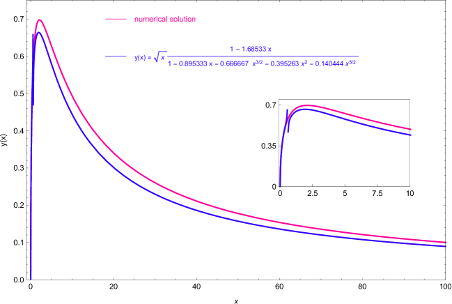
Figure 1: Our $y_{1,3}(x)$ in Eq. (4.16) vs. the numerical solution.

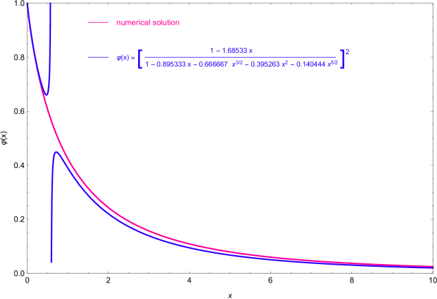
Figure 2: Our $\varphi_{1,3}(x)$ vs. the numerical solution.

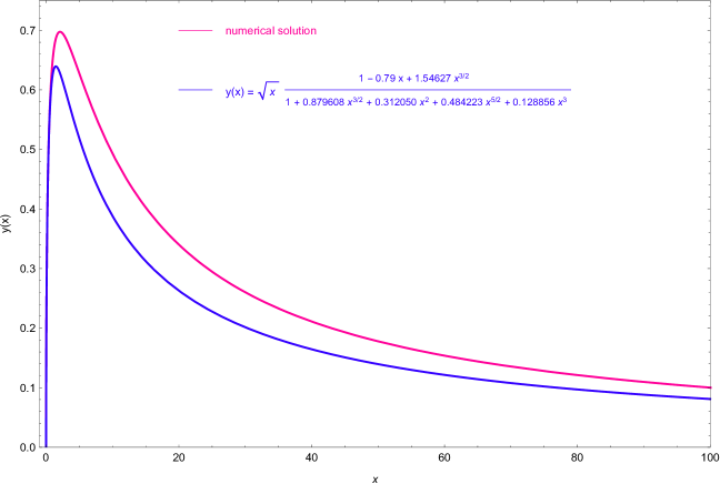
Figure 3: Our $y_{1,2}(x)$ in Eq. (4.17) vs. the numerical solution.

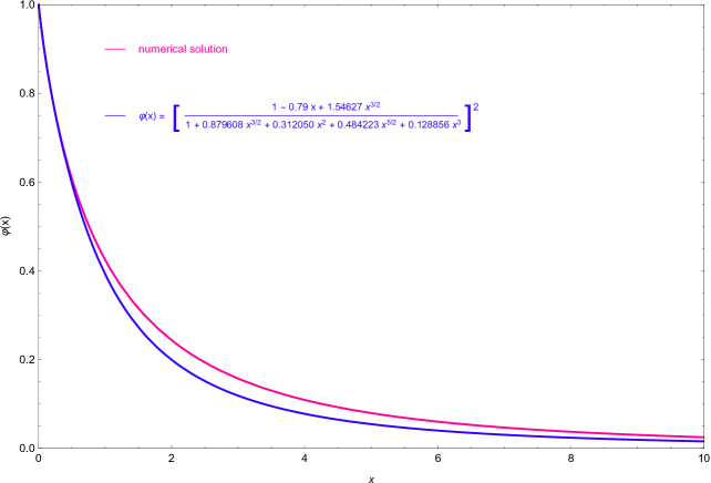
Figure 4: Our $\varphi_{1,2}(x)$ vs. the numerical solution.

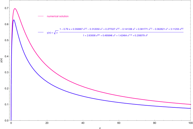
Figure 5: Our $y_{5,6}(x)$ from Eq. (4.5) vs. the numerical solution.

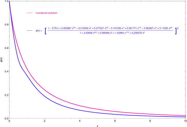
Figure 6: Our $\varphi_{5,6}(x)$ vs. the numerical solution.

Our findings are as follows. (i) Upon adding polynomial terms to numerator and denominator in the general formulae (4.3) and (4.5), the agreement between our approximate solutions and the numerical solutions starts worsening. More precisely, the additional terms lead to deviations from the numerical solutions at intermediate values of $x$, while for $x\rightarrow 0$ and $x\rightarrow\infty$ there is still good agreement. However, no conclusive evidence exists for the need to include or avoid bigger values of $l$ in Eqs. (4.3) and (4.5). (ii) As is clear from our plots, special attention must be payed to the interval of values of $x$ for which the denominator in Eqs. (4.16) and (4.17) approaches $0$. If we focus on $y(x)$ and on its pronounced maximum as the denominator approaches $0$, we discover that our approximate solution reproduces well such a feature, but there is no overlapping with the plot of the numerical solution.

6 Modern applications

The Thomas-Fermi equation has been applied and extended to many branches of modern physics until very recent times, including many-body systems in quantum mechanics [7, 8, 9], semiclassical theory of atoms [10], mathematical refinements [11, 12, 13], non-extensive statistical mechanics and relativistic formulation of the generalized non-extensive Thomas-Fermi model [13, 14]. In particular, we are here interested in the differential equation resulting from the latter framework. The work in Ref. [14] has proved that, upon defining the parameters

$$\alpha\equiv\left({4Z^{2}\over 3\pi}\right)^{2\over 3}{e^{4}\over\hbar^{2}c^{2}},$$ (6.1)

$$a\equiv\left({9\pi^{2}\over 128Z}\right)^{1\over 3}{\hbar^{2}\over me^{2}},$$ (6.2)

and denoting by $q$ the parameter that measures the departure of entropy from its additive nature in standard thermodynamics, one can further define the integrals

$$I_{n}^{(q)}\equiv q\int_{-\infty}^{\infty}{z^{n}[1+(q-1)z]^{1\over(q-1)}\over\left\{1+[1+(q-1)z]^{q\over(q-1)}\right\}^{2}}dz,$$ (6.3)

and the parameters ($T$ being the temperature in energy units)

$$\beta\equiv{3\over 2}TI_{1}^{(q)}{a\over e^{2}Z},$$ (6.4)

$$\gamma\equiv{3\over 8}T^{2}I_{2}^{(q)}{a^{2}\over e^{4}Z^{2}},$$ (6.5)

so that the desired generalized form of the Thomas-Fermi equation (1.2) reads as

$$\sqrt{x}{d^{2}\varphi\over dx^{2}}=\varphi^{3\over 2}\left[1+\alpha{\varphi\over x}\right]^{3\over 2}\left\{1+\beta{x\over\varphi}\left[1+\alpha{\varphi\over x}\right]^{-1}+\gamma{x^{2}\over\varphi^{2}}\left[1+\alpha{\varphi\over x}\right]^{-2}\right\}.$$ (6.6)

In this equation, relativistic effects are included by means of the $\alpha$ parameter, while non-extensive and thermal effects correspond to $\beta$ and $\gamma$, respectively [14]. It should be stressed that both non-extensive and thermal corrections depend on the $q$ parameter, that underpins the generalized entropy and is linked to the underlying dynamics of the atomic system while also providing a measure of the degree of its correlation.

At this stage, if we define the function $y$ as in Eq. (2.2), we obtain eventually the non-linear equation

$${d^{2}y\over dx^{2}}-{2\over x}{dy\over dx}+{y\over x^{2}}+{1\over y}\left({dy\over dx}\right)^{2}={1\over 2}{y^{2}\over x}F_{\alpha\beta\gamma}(x,y(x)),$$ (6.7)

having defined

$$f_{\alpha}(x,y(x))\equiv\left(1+\alpha{y^{2}\over x^{2}}\right),$$ (6.8)

$$F_{\alpha\beta\gamma}(x,y(x))\equiv f_{\alpha}^{3\over 2}\left[1+\beta{x^{2}\over y^{2}}f_{\alpha}^{-1}+\gamma{x^{4}\over y^{4}}f_{\alpha}^{-2}\right].$$ (6.9)

The desired approximate solution of Eq. (6.7) differs substantially from the Sommerfeld solution, as we will show in the following.

6.1 Small deviations from the Sommerfeld asymptotics

Let us look for an asymptotic expansion of the solution of the Thomas-Fermi equation in the limit $x\rightarrow\infty$. First of all, we will explore the inverse power law

$$y\sim\frac{k}{x^{\eta}}$$ (6.10)

for large $x$ and positive $\eta$ (corresponding to the physically relevant case of a vanishing electrostatic potential at large distances). As a first step, let us consider the standard Thomas-Fermi equation (6.7) with $F_{\alpha\beta\gamma}=1$; by substituting Eq. (6.10) into this equation we find:

$$\frac{2(2\eta^{2}+3\eta+1)}{x^{\eta+2}}=\frac{k}{x^{2\eta+1}},$$ (6.11)

which means that Eq. (6.10) yields a solution of the standard Thomas-Fermi equation provided that

$$\left\{\begin{array}[]{l}2(2\eta^{2}+3\eta+1)=k,\\ \eta+2=2\eta+1,\end{array}\right.\qquad\Longrightarrow\qquad\left\{\begin{array}[]{l}k=12,\\ \eta=1.\end{array}\right.$$ (6.12)

We then find the well-known result that the Sommerfeld solution $y\sim 12/x$ is the only inverse power-law solution of the standard Thomas-Fermi equation at large $x$.

Let us now restore the term $F_{\alpha\beta\gamma}\neq 1$ into Eq. (6.7); by substituting Eq. (6.10), and retaining only leading terms for large $x$, so that

$$F_{\alpha\beta\gamma}\sim 1+\frac{3}{2}\,\alpha\,\frac{k^{2}}{x^{2(\eta+1)}}+\beta\,\frac{x^{2(\eta+1)}}{k^{2}}\,+\,\gamma\,\frac{x^{4(\eta+1)}}{k^{4}}\sim\gamma\,\frac{x^{4(\eta+1)}}{k^{4}},$$ (6.13)

we obtain

$$\frac{2k^{3}(2\eta^{2}+3\eta+1)}{x^{\eta+2}}=\gamma\,{x^{2\eta+3}}.$$ (6.14)

This implies that, in order for Eq. (6.7) to be satisfied (in the large-$x$ limit) we should impose

$$\left\{\begin{array}[]{l}2k^{3}(2\eta^{2}+3\eta+1)=\gamma,\\ -\eta-2=2\eta+3,\end{array}\right.$$ (6.15)

finding therefore a negative $\eta=-5/3$, which of course does not correspond to an inverse power law. This means that non-standard effects in the modified Thomas-Fermi equation (6.7) prevent such a solution for large $x$ even, quite interestingly, just approximately for small (but finite) $\alpha,\beta,\gamma$ parameters. This result is not unexpected, since it results from the divergent part of $F_{\alpha\beta\gamma}$ for $y\sim k/x^{\eta}$, i.e., the last two terms in Eq. (6.9), that are proportional to $\beta$ and $\gamma$. A notable exception is the inclusion of only relativistic effects in the Thomas-Fermi equation, for which

$$F_{\alpha 00}\sim 1+{3\over 2}\,\alpha\,{y^{2}\over x^{2}}.$$ (6.16)

In such a case, however, the Sommerfeld solution $y\sim 12/x$ is only an approximate one for small values of the $\alpha$ parameter.

From a strictly physical viewpoint, we expect that the solution of the modified Thomas-Fermi equation (with $F_{\alpha\beta\gamma}\neq 1$) tends to that of the standard one (with $F_{\alpha\beta\gamma}=1$) for small values of the $\alpha,\beta,\gamma$ parameters. This has to be true also in the large-$x$ limit, so that, in such a limit, for $y\sim 12/x$ we should recover $F_{\alpha\beta\gamma}\sim 1$ for $\alpha,\beta,\gamma\rightarrow 0$. Now, since

$$\alpha\,{y^{2}\over x^{2}}\sim\alpha\,{144\over x^{4}}\rightarrow 0$$ (6.17)

for $x\rightarrow\infty$ independently of the value of $\alpha$ (so that $f_{\alpha}\rightarrow 1$ for $x\rightarrow\infty$), we should have

$$\beta\,{x^{2}\over y^{2}}+\gamma\,{x^{4}\over y^{4}}\rightarrow 0$$ (6.18)

in this limit, or, retaining only the leading term,

$$\gamma\,x^{4}\rightarrow 0.$$ (6.19)

Such a term effectively vanishes for $\gamma\rightarrow 0$, provided that the actual value of $x$ is not exceedingly large since, for fixed values of the parameter $\gamma$, $x$ might increase indefinitely. In other words, there should exist a large but finite value $x_{\infty}$ for which the asymptotic solution $y\sim 12/x$ holds as long as $x\ll x_{\infty}$. By contrast, notwithstanding $\gamma\rightarrow 0$, the condition (6.18) no longer holds in the opposite limit for ever increasing $x$ but, as long as we still approximately have $y\sim 12/x$, from the requirement that $F_{\alpha\beta\gamma}\sim 1$ for $x\sim x_{\infty}$ we now find

$$\gamma\,{x_{\infty}^{8}\over 12^{4}}\rightarrow 1.$$ (6.20)

We thus deduce that the cutoff value $x_{\infty}$,

$$x_{\infty}\sim\frac{\sqrt{12}}{\sqrt[8]{\gamma}},$$ (6.21)

diverges for $\gamma$ approaching zero, as expected.

Of course, for $x\gg x_{\infty}$ the asymptotic expression $y\sim 12/x$ is no longer valid and non-standard effects strongly affect the behaviour of $y(x)$, as we will see below.

6.2 Emergence of non-standard effects

The negative-$\eta$ solution of Eq. (6.15) would suggest a mathematical ansatz $y\sim s\,x^{\tau}$ with a positive power $\tau$, describing only non-standard effects for large $x$. However, following the same lines of reasoning as above, it is simple to show that similar contradictions as for (6.15) arise both for $0<\tau<1$ and for $\tau>1$, with the interesting exception of the case $\tau=1$. Indeed, by substituting

$$y\sim s\,x$$ (6.22)

into equation (6.7), we find that the modified Thomas-Fermi equation is satisfied provided that

$$0=\frac{1}{2}\,s^{2}xF_{\alpha\beta\gamma}.$$ (6.23)

Such a condition is actually fulfilled for $x\sim 0$ and any value of the non-standard parameters $\alpha,\beta,\gamma$, so that the linear function in Eq. (6.22) is an approximate solution of the modified Thomas-Fermi equation (for any value of $s$) in the small-$x$ regime, thus deviating appreciably from the $\sqrt{x}$ behaviour of the standard Thomas-Fermi case studied earlier.

By contrast, for finite $x$ (and $s$), from definition (6.9) the condition (6.23) leads to the requirement that the constant $s$ should satisfy the relation

$$\left(1+\alpha\,s^{2}\right)^{3/2}\left[1+\frac{\beta}{s^{2}(1+\alpha\,s^{2})}+\frac{\gamma}{s^{4}(1+\alpha\,s^{2})^{2}}\right]=0,$$ (6.24)

which displays a physically realizable solution. Indeed, for any value of the non-standard (positive) parameters $\alpha,\beta,\gamma$, we obtain $s=s_{\ast}$, with

$$s_{\ast}=\sqrt{\frac{1}{2\alpha}\left[\sqrt{1+2\alpha\left(\sqrt{\beta^{4}+4\gamma^{2}}-\beta\right)}-1\right]}.$$ (6.25)

Thus, the linear solution (6.22) effectively rules strong non-standard effects, for which $F_{\alpha\beta\gamma}$ vanishes rather than approaching the unit value.

6.3 Small-$x$ solutions

Non-standard effects resulting from a linear behaviour (underlying a vanishing $F_{\alpha\beta\gamma}$ term) for finite $x$ are even more pronounced in the neighborhood of the origin. This can be explored by looking for an approximate solution in the form

$$y\sim Q\,x^{\tau},$$ (6.26)

for $x\rightarrow 0$ and positive $\tau$. It is straightforward to see that in the small $x$-regime, for $\tau<1$, we recover the square root behaviour (corresponding to $\tau=1/2$) for vanishing values of the $\alpha$ parameter, by simply substituting Eq. (6.26) into the modified Thomas-Fermi equation (6.7). However, for finite values of the non-standard parameters (mainly ruled by $\gamma$, as we will see), the small-$x$ behaviour manifests itself into a different, larger value of the exponent. Again, substitution of Eq. (6.26) into Eq. (6.7) leads for $\tau>1$ to the equation

$$\frac{2Q^{3}(2\tau^{2}-3\tau+1)}{x^{2-\tau}}=\frac{\gamma}{x^{2\tau-3}},$$ (6.27)

when retaining only the leading terms, which is actually satisfied provided that

$$\left\{\begin{array}[]{l}\displaystyle 2Q^{3}(2\tau^{2}-3\tau+1)=\gamma,\\ \displaystyle 2-\tau=2\tau-3,\end{array}\right.\qquad\Longrightarrow\qquad\left\{\begin{array}[]{l}\displaystyle Q=Q_{\ast}\equiv\sqrt[3]{\frac{9\gamma}{28}}\,,\\ \\ \displaystyle\tau=\frac{5}{3}.\end{array}\right.$$ (6.28)

Note that, in the small-$x$ regime, such a solution corresponds to a large value of the $F_{\alpha\beta\gamma}$ term in the modified Thomas-Fermi equation that, although signaling a non-standard behaviour ($F_{\alpha\beta\gamma}\neq 1$), is at variance with the linear solution underpinning a vanishing $F_{\alpha\beta\gamma}$ term. However, as for the linear case, such $x^{5/3}$ behaviour is again ruled by thermal effects by means of a finite value of the $\gamma$ parameter.

7 Concluding remarks

Our sections 2-5 have been devoted to a detailed investigation of the non-relativistic Thomas-Fermi boundary-value problem. As far as we know, our auxiliary differential equation (2.6), the form (3.4)-(3.6) of the boundary conditions, and the two families of approximate solutions in Eq. (4.10) are completely new, as well as the particular examples in Eqs. (4.16) and (4.17). The fairly good agreement with the numerical solution, displayed in the plots of Section 5, is encouraging. Moreover, the smooth transition from the small-$x$ to the large-$x$ behaviour is another merit of our original approximate solutions.

In section $6$, we have instead investigated the joint effect of relativistic, non-extensive and thermal effects in the Thomas-Fermi equation, and we have discovered the following approximate power-law behaviours for the solution of the modified Thomas-Fermi equation in the different regimes:

$$\begin{array}[]{rlll}{\rm small}\,x:&\quad y\sim k\,\sqrt{x},&\quad{\rm small}\,\alpha,&\quad{\rm arbitrary}\,F_{\alpha\beta\gamma};\\ \\ {\rm small}\,x:&\quad\displaystyle y\sim Q_{\ast}\,x^{5/3},&\quad{\rm finite}\,\alpha,\beta,\gamma,&\quad{\rm large}\,F_{\alpha\beta\gamma};\\ \\ {\rm finite}\,x:&\quad\displaystyle y\sim s_{\ast}\,x,&\quad{\rm finite}\,\alpha,\beta,\gamma,&\quad{\rm small}\,F_{\alpha\beta\gamma};\\ \\ \begin{array}[]{r}{\rm large}\,x:\\ \left[x\ll x_{\infty}\right]\end{array}\!\!&\quad\displaystyle y\sim\frac{12}{x},&\quad{\rm small}\,\beta,\gamma,&\quad{\rm unit}\,F_{\alpha\beta\gamma};\end{array}$$

The original calculations of our work provide encouraging evidence in favour of the Thomas-Fermi equation being a valuable source of inspiration for understanding the wide range of modern applications [15, 16, 17, 18, 19] of atomic physics.

References

- [1] L.H. Thomas, The calculations of atomic fields, Proc. Cambridge Philos. Soc. 23, 542-598 (1927).
- [2] E. Fermi, Eine statistiche methode zur bestimmung einiger eigenschaften des atoms und ihre anwendung auf die theories des periodischen systems der elemente, Z. Phys. 48, 73-79 (1928).
- [3] S. Esposito, E. Majorana Jr., A. van der Merwe, E. Recami, Ettore Majorana: Notebooks in Theoretical Physics (Kluwer, Dordrecht, 2003).
- [4] E Di Grezia and S. Esposito, Fermi, Majorana and the statistical model of atoms, Found. Phys. 34, 1431-1450 (2004).
- [5] S. Esposito, Majorana solution of the Thomas-Fermi equation, Am. J. Phys. 70, 852-856 (2002).
- [6] A. Sommerfeld, Integrazione asintotica dell’equazione differenziale di Thomas-Fermi, Rend. R. Accademia dei Lincei 15, 293-308 (1932).
- [7] J. Sanudo, A.F. Pacheco, Electrons in a box: Thomas-Fermi solution, Can. J. Phys. 84, 833 (2006).
- [8] R.J. Komlos, A. Rabinovitch, Thomas-Fermi model for quasi one-dimensional finite crystals, Phys. Lett. A 372, 6670 (2008).
- [9] W. Wilcox, Thomas-Fermi statistical models of finite quark matter, Nucl. Phys. A 826, 49 (2009).
- [10] B.G. Englert, Semiclassical Theory of Atoms (Springer, Berlin, 1988).
- [11] E. Martinenko, B.K. Shamoggi, Thomas-Fermi model: Nonextensive statistical mechanics approach, Phys. Rev. A 69, 52504 (2004).
- [12] A. Nagy, E. Romera, Maximum Rényi entropy and the generalized Thomas-Fermi model, Phys. Lett. A 373, 844 (2009).
- [13] K. Ourabah, M. Tribeche, The nonextensive Thomas-Fermi theory in an -dimensional space, Physica A 392, 4477-4480 (2013).
- [14] K. Ourabach, M. Tribeche, Relativistic formulation of the generalized nonextensive Thomas-Fermi model, Physica A 393, 470-474 (2014).
- [15] H. Shababi, K. Ourabah, Thomas-Fermi theory at the Planck scale: A relativistic approach, Ann. Phys. (N.Y.) 413, 168051 (2020).
- [16] M. Ghozanfari Mojamad, J. Ranjbar, Thomas-Fermi approximation in the phase transition of neutron star matter from -stable nuclear matter to quark matter, Ann. Phys. (N.Y.) 412, 168048 (2020).
- [17] S. Kumar Roy, S. Mukhopadhyay, J. Lahiri, D.N. Basu, Relativistic Thomas-Fermi equation of state for magnetized white dwarfs, Phys. Rev. D 100, 063008 (2019).
- [18] M. Ghazanfari Mojarrad, J. Ranjbar, Hybrid neutron stars in the Thomas-Fermi theory, Phys. Rev. C 100, 015804 (2019).
- [19] K. Pal, L. V. Sales, J. Wudka, Ultralight Thomas-Fermi dark matter, Phys. Rev. D 100, 083007 (2019).