Augmented resolution of linear hyperbolic systems under nonconservative form

Abstract

Hyperbolic systems under nonconservative form arise in numerous applications modeling physical processes, for example from the relaxation of more general equations (e.g. with dissipative terms). This paper reviews an existing class of augmented Roe schemes and discusses their application to linear nonconservative hyperbolic systems with source terms. We extend existing augmented methods by redefining them within a common framework which uses a geometric reinterpretation of source terms. This results in intrinsically well-balanced numerical discretizations. We discuss two equivalent formulations: (1) a nonconservative approach and (2) a conservative reformulation of the problem. The equilibrium properties of the schemes are examined and the conditions for the preservation of the well-balanced property are provided. Transient and steady state test cases for linear acoustics and hyperbolic heat equations are presented. A complete set of benchmark problems with analytical solution, including transient and steady situations with discontinuities in the medium properties, are presented and used to assess the equilibrium properties of the schemes. It is shown that the proposed schemes satisfy the expected equilibrium and convergence properties.

Key words: Augmented Roe solver, nonconservative system, moving equilibria, well-balanced scheme

1 Introduction

In this work, our aim is to give a detailed overview of using augmented solvers for linear nonconservative hyperbolic systems, with an emphasis on preserving exact (moving) equilibria. The preservation of such equilibria is an issue of paramount importance since many events of interest are just perturbations of an equilibrium state. However, especially in the presence of source terms, preserving the correct equilibrium is numerically challenging. Schemes that recover these solutions exactly are referred to as well-balanced schemes [2]. General frameworks to design well-balanced numerical schemes for nonlinear nonconservative systems have been developed in, for example, [22, 15]. These frameworks are based on the so-called path-conservative methods. In contrast, we will design our framework based on the augmented solver methods [19]. These augmented solver-based schemes have been successfully applied to various hyperbolic conservation and balance laws, see, for example, [18], but have not yet been discussed in the context of nonconservative systems.

In the following, we will consider linear systems of partial differential equations in the form of

$$\frac{\partial U}{\partial t}+\mathcal{A}\left(x\right)\frac{\partial U}{\partial x}=S,$$ (1)

where $U=U\left(x,t\right)\in\Xi\subset\mathbb{R}^{n}$ is the vector of conserved quantities that takes values on $\Xi$, the set of admissible states of $U$, $\mathcal{A}=\mathcal{A}\in\mathbb{R}^{n\times n}$ is a variable coefficient matrix, and $S$ is the vector of sources, which will be considered to be of the form $S=S\left(U\right)$. $n$ denotes the number of equations and unknowns. The domain of definition for the problem in Eq. (1) is given by $\Psi=\Omega\times\left[0,T\right]$, hence $x\in\Omega\subset\mathbb{R}$.

The system in Eq. (1) is said to be hyperbolic, if $\forall x\in\Omega\subset\mathbb{R}$ and $\forall U\in\Xi$, the matrix $\mathcal{A}$ is diagonalizable with $n$ real eigenvalues. If the eigenvalues are distinct, then the system is said to be strictly hyperbolic [8]. Further, the system in Eq. (1) is considered nonconservative, if the matrix $\mathcal{A}\in\mathbb{R}^{n\times n}$ is not assumed to be a Jacobian matrix of a conservative flux [6]. Hyperbolic partial differential equations often arise from the relaxation of more general problems, such as those involving dissipative terms. In these cases, the issue of having infinite wave speeds associated with the diffusive terms is resolved.

The ability of a numerical scheme to preserve the correct equilibrium is closely related to the equilibrium condition across a discontinuity. This condition can be derived by integrating Eq. (1) inside a sufficiently large spatial domain. Consider the discontinuous solution of Eq. (1), located at $x=x_{d}$ at the initial time $t=0$, defined as

$$U\left(x,t\right)=\begin{cases}U_{L}&\text{if }x<x_{d}+\sigma t,\\ U_{R}&\text{if }x>x_{d}+\sigma t,\end{cases}$$ (2)

where the subscripts $L$ and $R$ denote the left and right hand-side of the discontinuity, and $\sigma$ is the wave celerity. Using an integration volume $\left[x_{L},x_{R}\right]\in\mathbb{R}$ such that $x_{L}<x_{d}<x_{R}$, the integration of Eq. (1) inside this volume yields

$$\int_{x_{L}}^{x_{R}}\mathcal{A}\left(x\right)\frac{\partial U}{\partial x}dx-\sigma\left(U_{R}-U_{L}\right)=\int_{x_{L}}^{x_{R}}S\left(U\right)dx.$$ (3)

Eq. (3) is only satisfied if the source term is considered to be a singular source defined at $x_{d}$ at the initial time that travels with the wave—its position in time is given by $x_{d}+\sigma t$) [13]. In what follows, source terms will be considered to be defined at fixed locations—in other words, not traveling with the wave. Thus, for traveling waves, Eq. (3) reduces to

$$\int_{x_{L}}^{x_{R}}\mathcal{A}\left(x\right)\frac{\partial U}{\partial x}dx-\sigma\left(U_{R}-U_{L}\right)=0.$$ (4)

For steady waves with $\sigma=0$, Eq. (3) reduces to

$$\int_{x_{L}}^{x_{R}}\mathcal{A}\left(x\right)\frac{\partial U}{\partial x}dx=\int_{x_{L}}^{x_{R}}S\left(U\right)dx.$$ (5)

This separation leads to the generalized Rankine-Hugoniot relation (GRH) in the steady state, which are a keystone in the construction of augmented solvers.

The methods herein used focus on the resolution of non-conservative systems with geometric source terms, defined as a function of the system variables and the gradient of a scalar field. In contrast, nongeometric source terms do not include such a gradient in their definition.

In what follows, we will redefine augmented schemes to solve arbitrary linear hyperbolic systems under nonconservative form. For well-balancing purposes, we use a geometric reinterpretation of source terms, which is a generalization of the idea introduced in [3]. In this method, source terms are considered in the Riemann problem as singular sources in the sense of distributions. Our generalization of this method allows to obtain well-balanced properties even in cases with nongeometrical source terms. In combination with augmented Riemann solvers, this source term treatment enables exact equilibrium solutions for linear hyperbolic systems.

We present two equivalent forms of this numerical scheme: (1) the fluctuation form and (2) the numerical flux form. The fluctuation form of our approach can be directly applied to the nonconservative system. The numerical flux form requires rewriting the system by augmenting with additional equations accounting for the variation in time of the system matrix coefficients and additional source terms. In this way, a conservative flux can be defined and the scheme can be written in numerical flux form.

We apply these schemes to the linear acoustic equations and to the hyperbolized heat equation with source term. The latter involves a stiff relaxation source term which must be exactly balanced in order to provide a conservative estimation of the heat flux. A complete set of steady and transient test cases are presented together with their analytical solution. To emphasize the importance of well-balancing, the solution provided by the well-balanced schemes is compared with the solution provided by a wave propagation algorithm that uses a centered explicit—that is to say not well-balanced—integration of source terms.

2 Numerical resolution of nonconservative systems

Consider the Cauchy problem defined in the domain $\Omega\times[0,T]$ for the partial differential equation in Eq. (1) with

$$\left\{\begin{aligned} &\text{IC: }U\left(x,0\right)=\accentset{\circ}{U}\left(x\right),\;\forall x\in\Omega,\\ &\text{BC: }U\left(x,t\right)=U_{\partial\Omega}\left(x,t\right)\;\forall x\in\partial\Omega,\end{aligned}\right.$$ (6)

where IC denotes the initial condition specified by a suitable function $\accentset{\circ}{U}\left(x\right):\Omega\rightarrow\Xi$, and BC denotes the boundary condition specified by a suitable function $U_{\partial\Omega}\left(x,t\right):\Omega\times[0,T]\rightarrow\Xi$. The spatial domain is given by $\Omega=\left[a,b\right]$, with $a$ and $b$ being the start and end points of the domain, respectively. It is discretized in $N$ volume cells, defined as $\Omega_{i}\subseteq\Omega$, such that $\Omega\approx\Omega_{\Delta x}=\bigcup_{i=1}^{N}\Omega_{i}$, with cell edges at

$$a=x_{\frac{1}{2}}<x_{\frac{3}{2}}<...<x_{N-\frac{1}{2}}<x_{N+\frac{1}{2}}=b,$$ (7)

and with cell size $\Delta x$. In the following, we assume that the discretized domain $\Omega_{\Delta x}$ is identical to $\Omega$. Inside each cell, at time $t^{n}$, the conserved quantities are defined as cell averages as

$$U_{i}^{n}=\frac{1}{\Delta x}\int_{x_{i-\frac{1}{2}}}^{x_{i+\frac{1}{2}}}U\left(x,t^{n}\right)dx,\quad i=1,\dots,N.$$ (8)

Integration of the system in Eq. (6) inside the control volume $\Omega_{i}\times\left[t^{n},t^{n+1}\right]$ yields Godunov’s scheme [9]

$$U_{i}^{n+1}=U_{i}^{n}-\frac{\Delta t}{\Delta x}\left(D_{i+\frac{1}{2}}^{-}+D_{i-\frac{1}{2}}^{+}\right)^{n}+{\Delta t}\bar{S}_{i}^{n},$$ (9)

where $D_{i+\frac{1}{2}}^{-}$ and $D_{i-\frac{1}{2}}^{+}$ are the nonconservative fluctuations, and $\bar{S}_{i}$ is the numerical approximation of the integral of the source term as

$$\bar{S}_{i}\approx\int_{x_{i-\frac{1}{2}}}^{x_{i+\frac{1}{2}}}S\left(U\right)dx.$$ (10)

$D_{i+\frac{1}{2}}^{-}$ and $D_{i-\frac{1}{2}}^{+}$ are computed by solving the Riemann problem (RP) for Eq. (1) across the interfaces $i+\frac{1}{2}$ and $i-\frac{1}{2}$ of the cell, respectively. For example, at the interface $i+\frac{1}{2}$, the RP is

$$\accentset{\circ}{U}\left(x\right)=\begin{cases}U_{i}&\text{if }x<x_{i+\frac{1}{2}},\\ U_{i+1}&\text{if }x>x_{i+\frac{1}{2}}.\end{cases}$$ (11)

Let us study the conditions that such a numerical scheme must satisfy to preserve equilibrium states. Consider the FV discretization of cell values in Eq. (8). In order to preserve an initial steady state, the equilibrium condition in Eq. (5) must be satisfied at each cell interface. Across a discontinuity at an interface $i+\frac{1}{2}$, the integration of Eq. (1) on $\left[x_{i},x_{i+1}\right]$ gives

$$\int_{x_{i}}^{x_{i+1}}\mathcal{A}\left(x\right)\frac{\partial U}{\partial x}dx=\int_{x_{i}}^{x_{i+1}}S\left(U\right)dx.$$ (12)

The integral of the nonconservative products on the left hand side of Eq. (12) can be approached as

$$\int_{x_{i}}^{x_{i+1}}\mathcal{A}\left(x\right)\frac{\partial U}{\partial x}dx=\left(\widetilde{\mathcal{A}}\delta U\right)_{i+\frac{1}{2}},$$ (13)

where

$$\widetilde{\mathcal{A}}_{i+\frac{1}{2}}=\frac{1}{2}\left(\mathcal{A}_{i}+\mathcal{A}_{i+1}\right),$$ (14)

and $\delta U_{i+\frac{1}{2}}=U_{i+1}-U_{i}$. This allows to rewrite Eq. (12) as

$$\left(\widetilde{\mathcal{A}}\delta U\right)_{i+\frac{1}{2}}=\int_{x_{i}}^{x_{i+1}}S\left(U\right)dx.$$ (15)

In order to preserve the equilibrium state, suitable numerical approximations to the integral of the source term that depend on both the form of the fluctuations and the source term must be derived to satisfy Eq. (15). We see that the traditional finite volume (FV) updating scheme in Eq. (9) in combination with Eq. (10) does not intrinsically preserve equilibria, because we have not specified how the integration is carried out. Hence, the integral of the source term is not guaranteed to satisfy Eq. (15) at cell interfaces.

Finding suitable approximations that satisfy Eq. (15) is a subtle issue, commonly studied in depth-averaged geophysical flow modeling, see for example [1, 2, 18, 29]. In this context, a geometric reinterpretation of the source term $S\left(U\right)$ yields a well-balanced numerical scheme with the nature of the source term [3].

2.1 Geometric reinterpretation of source terms

The nonconservative products in Eq. (15) may be exactly balanced with the source terms using a geometric reinterpretation of $S\left(U\right)$ as

$$S\left(U\right)=\frac{\partial}{\partial x}V\left(x,S\right).$$ (16)

Here, $V$ is the primitive variable of $S\left(U\right)$ that satisfies

$$V\left(x,S\right)=\int_{-\infty}^{x}S\left(U\right)dx.$$ (17)

If the piecewise constant FV discretization of data, given in Eq. (8), is also applied to the source term, $V$ can be evaluated at the cell interfaces as

$$\left\{\begin{aligned} &V_{i+\frac{1}{2}}=V\left(0\right)+\sum_{\iota=1}^{i}S_{\iota}\Delta x,\\ &S_{i}=\frac{1}{\Delta x}\int_{x_{i-\frac{1}{2}}}^{x_{i+\frac{1}{2}}}S\left(U\right)dx,\end{aligned}\right.$$ (18)

where we set $V\left(0\right)=0$ for the sake of simplicity. If considering a linear approximation, cell averages of the primitive variable $V$ can computed as

$$V_{i}=\frac{1}{2}\left(V_{i+\frac{1}{2}}+V_{i-\frac{1}{2}}\right),$$ (19)

which can also be written as

$$V_{i}=V_{i-\frac{1}{2}}+\frac{1}{2}S_{i}\Delta x.$$ (20)

Using Eq. (20), we define

$$\delta V_{i+\frac{1}{2}}=V_{i+1}-V_{i}=V_{i+\frac{1}{2}}+\frac{1}{2}S_{i+1}\Delta x-V_{i-\frac{1}{2}}-\frac{1}{2}S_{i}\Delta x.$$ (21)

The integral of the source term in Eq. (15), hereafter referred to as integral of the source term at the interface, can be approached by using Eq. (16) as

$$\left\{\begin{aligned} \bar{S}_{i+\frac{1}{2}}&=\int_{x_{i}}^{x_{i+1}}S\left(U\right)dx,\\ &=\int_{x_{i}}^{x_{i+1}}\frac{\partial}{\partial x}V\left(x,S\right)dx,\\ &\approx\delta V_{i+\frac{1}{2}}\equiv\frac{1}{2}\left(S_{i}+S_{i+1}\right)\Delta x,\end{aligned}\right.$$ (22)

provided a linear approximation. Note that the degree of the approximation for $V_{i}$ will have an impact on the overall order of the numerical scheme (e.g. the linear approximation in Eq. (19) yields a second order of accuracy). Moreover, when dealing with nonlinear systems and source terms, a more sophisticated averaging for Eq. (19) might be required.

The steady equilibrium condition that relates the discontinuous left and right states at the interface $i+\frac{1}{2}$ given by Eq. (12) can be obtained by combining Eq. (15) with Eq. (22) as

$$\left(\widetilde{\mathcal{A}}\delta U\right)_{i+\frac{1}{2}}=\delta V_{i+\frac{1}{2}},$$ (23)

which states that the jump across cell interfaces under steady state is

$$\delta U_{i+\frac{1}{2}}=\frac{1}{2}\widetilde{\mathcal{A}}^{-1}\left(S_{i+1}+S_{i}\right)\Delta x.$$ (24)

Proposition 2.1

For a numerical scheme that satisfies the approximate GRH relation in Eq. (12) at cell interfaces and considers the linear approximation of the nonconservative product and source term in Eq. (15) and Eq. (22), respectively, the numerical solution of Eq. (1) will be equal to the analytical solution (considering machine accuracy) iff for the analytical solution of Eq. (1), $\mathcal{A}\left(U\right)\frac{\partial U}{\partial x}$ can be expressed as a polynomial of degree at most 1 ($\mathcal{A}\left(x\right)\frac{\partial U}{\partial x}\in P_{1}(\Omega)$), with $P_{1}$ the degree 1-polynomial basis and $x\in\Omega$, and at the same time $S$ can also be expressed as a polynomial of degree at most 1 ($S\in P_{1}(\Omega)$).

Proof 2.1

Since the linear approximation of the nonconservative products and source term in Eq. (15) and Eq. (22), respectively, provide the exact integral if those terms are polynomials of degree at most one, the exact GRH relation in Eq. (12) is recovered at every cell interface and the exact solution is thus obtained. Since the linear approximation of the nonconservative products and source term can not ensure an exact integral if those terms are polynomials of degree higher than one, the exact GRH relation in Eq. (12) can not be recovered, and the numerical solution deviates from the exact solution. Prop. 2.1 is thus proved.

Corollary 2.1.1

Let us consider a numerical scheme for the resolution of Eq. (1) that satisfies the approximate GRH relation in Eq. (12) at cell interfaces and considers the linear approximation of the nonconservative products and source term in Eq. (15) and Eq. (22), respectively. Let $q$ be a variable of the system in Eq. (12), that represents a physical conservative flux. Further, let $q$ satisfy $\partial q/\partial t=0$ and $\partial q/\partial x=\phi$ at the steady state, where $\phi$ (e.g., a source of the quantity associated to $q$), is a polynomial of degree at most 1 ( $\phi\in P_{1}(\Omega)$). Then, the numerical scheme will preserve the exact conservation of $q$ at the discrete level under steady state. The conditions $\partial q/\partial t=0$ and $\partial q/\partial x=\phi$ will be fulfilled with machine accuracy.

We will now discuss how to combine this source term treatment with augmented solvers to obtain a well-balanced numerical scheme.

2.2 Augmented resolution of the nonhomogeneous system

The augmented Riemann solver approach is based on the consideration of the source terms directly in the definition of the Riemann problem as a singular source term. This way, the contribution of the source term is not explicitly included in the updating scheme for the problem in Eq. (6), but in the definition of the fluctuations, yielding

$$U_{i}^{n+1}=U_{i}^{n}-\frac{\Delta t}{\Delta x}\left(D_{i+\frac{1}{2}}^{-}+D_{i-\frac{1}{2}}^{+}\right)^{n}.$$ (25)

The fluctuations must satisfy

$$D_{i+\frac{1}{2}}^{-}+D_{i+\frac{1}{2}}^{+}=\int_{x_{i}}^{x_{i+1}}\mathcal{A}\left(x\right)\frac{\partial U}{\partial x}dx-\int_{x_{i}}^{x_{i+1}}S\left(U\right)dx$$ (26)

for a suitable approximation of the integrals of the nonconservative product and the source term. Since we directly average the coefficient matrix, and use the geometric reinterpretation of the source term in Eq. (22), Eq. (26) becomes

$$D_{i+\frac{1}{2}}^{-}+D_{i+\frac{1}{2}}^{+}=\left(\widetilde{\mathcal{A}}\delta U-\delta V\right)_{i+\frac{1}{2}},$$ (27)

which recovers the equilibrium condition in Eq. (23) at the steady state. In the following, the fluctuations, $D_{i+\frac{1}{2}}^{-}$ and $D_{i-\frac{1}{2}}^{+}$, are derived following two equivalent approaches. The first approach is based on the resolution of the nonconservative system, allowing to satisfy Eq. (27) by decomposing the source term in the system matrix eigenvector basis. It is referred to as the fluctuation form of the augmented scheme. The second approach is based on rewriting the system in conservative form by introducing the definition of a conservative flux. In this way, the updating scheme can be written in numerical flux form and Eq. (27) will be satisfied by decomposing the source term using the eigenvector basis of the Jacobian of the conservative flux. Consequently, we refer to this approach as the flux form of the augmented scheme.

2.2.1 Augmented scheme in fluctuation form

We consider the RP in Eq. (11) for the hyperbolic system in Eq. (1), and approximate it by a constant coefficient linear RP as

$$\left\{\begin{aligned} &\text{PDE: }\frac{\partial\hat{U}}{\partial t}+\widetilde{\mathcal{A}}_{i+\frac{1}{2}}\frac{\partial\hat{U}}{\partial x}=\bar{S}_{i+\frac{1}{2}}\delta_{x=x_{i+1/2}},\\ &\text{IC: }\accentset{\circ}{\hat{U}}\left(x\right)=\begin{cases}U_{i}&\text{if }x<x_{i+\frac{1}{2}},\\ U_{i+1}&\text{if }x>x_{i+\frac{1}{2}},\end{cases}\end{aligned}\right.$$ (28)

where $\widetilde{\mathcal{A}}_{i+\frac{1}{2}}$ is computed using the linear averaging in Eq. (14), $\hat{U}\left(x,t\right)$ is the approximate solution of the RP in Eq. (11) for Eq. (1), and the singular source term is defined as

$$\bar{S}_{i+\frac{1}{2}}\delta_{x=x_{i+1/2}}=\begin{cases}\delta V_{i+\frac{1}{2}}&\text{if }x=x_{i+\frac{1}{2}},\\ 0&\text{else},\end{cases}$$ (29)

allowing to recover the GRH condition in Eq. (23) at the interface. Note that $\delta_{x=x_{i+1/2}}$ is the Dirac mass placed at $x_{i+\frac{1}{2}}$. Since in our case linear averaging of $\mathcal{A}$ yields a Roe-type matrix [23], $\widetilde{\mathcal{A}}_{i+\frac{1}{2}}$ is diagonalizable with ${N_{\lambda}}=n$ real eigenvalues $\widetilde{\lambda}^{m}_{i+\frac{1}{2}}$ and right eigenvectors $\widetilde{e}^{m}$ that approximate the eigenvalues and eigenvectors of $\mathcal{A}$ from the original RP in Eq. (11). Using $\widetilde{\lambda}^{m}_{i+\frac{1}{2}}$ and $\widetilde{e}^{m}$, we can construct the matrix $\widetilde{\mathcal{P}}_{i+\frac{1}{2}}=\left[\widetilde{e}^{1},\widetilde{e}^{2},\dots,\widetilde{e}^{N_{\lambda}}\right]$ and its inverse $\widetilde{\mathcal{P}}^{-1}_{i+\frac{1}{2}}$. Then, $\widetilde{\mathcal{A}}_{i+\frac{1}{2}}$ can be diagonalized as

$$\widetilde{\mathcal{A}}_{i+\frac{1}{2}}=\left(\widetilde{\mathcal{P}}\widetilde{\Lambda}\widetilde{\mathcal{P}}\right)_{i+\frac{1}{2}},$$ (30)

where $\widetilde{\Lambda}_{i+\frac{1}{2}}=\text{diag}\left(\widetilde{\lambda}^{1},\widetilde{\lambda}^{2},\dots,\widetilde{\lambda}^{N_{\lambda}}\right)$ is a diagonal matrix with the approximate eigenvalues as entries.

The system in Eq. (28) can now be decoupled as

$$\left\{\begin{aligned} &\text{PDE: }\frac{\partial\hat{W}}{\partial t}+\widetilde{\Lambda}_{i+\frac{1}{2}}\frac{\partial\hat{W}}{\partial x}=\bar{B}_{i+\frac{1}{2}}\delta_{x=x_{i+1/2}},\\ &\text{IC: }\accentset{\circ}{\hat{W}}\left(x\right)=\begin{cases}W_{i}=\widetilde{\mathcal{P}}^{-1}_{i+\frac{1}{2}}U_{i}&\text{if }x<x_{i+\frac{1}{2}},\\ W_{i+1}=\widetilde{\mathcal{P}}^{-1}_{i+\frac{1}{2}}U_{i+1}&\text{if }x>x_{i+\frac{1}{2}},\end{cases}\end{aligned}\right.$$ (31)

where $\hat{W}=\widetilde{\mathcal{P}}^{-1}_{i+\frac{1}{2}}\hat{U}$ are the characteristic variables, $\hat{W}=\left[\hat{w}^{1},\hat{w}^{2},\dots,\hat{w}^{N_{\lambda}}\right]$, and $\bar{B}_{i+\frac{1}{2}}=\widetilde{\mathcal{P}}^{-1}_{i+\frac{1}{2}}\bar{S}_{i+\frac{1}{2}}$ is the projection of the source term onto the eigenbasis of the coefficient matrix $\widehat{\mathcal{A}}$.

The general solution $\hat{U}\left(x,t\right)$ can be derived by expanding the solution as a linear combination of the eigenvectors as

$$\hat{U}\left(x,t\right)=\sum_{m=1}^{N_{\lambda}}\hat{w}^{m}\left(x,t\right)\widetilde{e}^{m}_{i+\frac{1}{2}},$$ (32)

where the scalar values $\hat{w}^{m}(x,t)$ are the characteristic solutions and represent the strength of each $m$-wave.

Let $U^{-}_{i+\frac{1}{2}}$ and $U^{+}_{i+\frac{1}{2}}$ be the left and right states in the vicinity of $x_{i+\frac{1}{2}}$, respectively, defined as

$$\left\{\begin{aligned} U^{-}_{i+\frac{1}{2}}=\lim_{x\rightarrow x_{i+\frac{1}{2}}^{-}}\hat{U}\left(x,t\right),\\ U^{+}_{i+\frac{1}{2}}=\lim_{x\rightarrow x_{i+\frac{1}{2}}^{+}}\hat{U}\left(x,t\right),\end{aligned}\right.$$ (33)

They can be computed as shown in [19] as

$$\left\{\begin{aligned} &U^{-}_{i+\frac{1}{2}}=U_{i}+\sum_{\lambda^{m}<0}\left[\left(\alpha-\frac{\bar{\beta}}{\widetilde{\lambda}}\right)\widetilde{e}\right]^{m}_{i+{\frac{1}{2}}},\\ &U^{+}_{i+\frac{1}{2}}=U_{i+1}-\sum_{\lambda^{m}>0}\left[\left(\alpha-\frac{\bar{\beta}}{\widetilde{\lambda}}\right)\widetilde{e}\right]^{m}_{i+{\frac{1}{2}}},\end{aligned}\right.$$ (34)

where the set of wave and source strengths, $\vec{\alpha}$ and $\vec{\beta}$, respectively, are defined as

$$\left\{\begin{aligned} &\vec{\alpha}_{i+\frac{1}{2}}=\left[\alpha^{1},\alpha^{2},\dots,\alpha^{N_{\lambda}}\right]^{T}_{i+{\frac{1}{2}}}=\left(\widetilde{\mathcal{P}}^{-1}\delta U\right)_{i+\frac{1}{2}},\\ &\vec{\beta}_{i+\frac{1}{2}}=\left[\beta^{1},\beta^{2},\dots,\beta^{N_{\lambda}}\right]_{i+\frac{1}{2}}^{T}=\left(\widetilde{\mathcal{P}}^{-1}\delta V\right)_{i+\frac{1}{2}}.\end{aligned}\right.$$ (35)

The fluctuations are calculated as

$$\left\{\begin{aligned} D_{i+\frac{1}{2}}^{-}=\sum_{\lambda^{m}<0}\left[\left(\widetilde{\lambda}\alpha-\beta\right)\widetilde{e}\right]^{m}_{i+\frac{1}{2}},\\ D_{i+\frac{1}{2}}^{+}=\sum_{\lambda^{m}>0}\left[\left(\widetilde{\lambda}\alpha-\beta\right)\widetilde{e}\right]^{m}_{i+\frac{1}{2}}.\end{aligned}\right.$$ (36)

This satisfies

$$\delta V_{i+\frac{1}{2}}=\widetilde{\mathcal{A}}_{i+\frac{1}{2}}\left(U^{+}_{i+\frac{1}{2}}-U^{-}_{i+\frac{1}{2}}\right),$$ (37)

which under steady state yields

$$\delta V_{i+\frac{1}{2}}=\widetilde{\mathcal{A}}_{i+\frac{1}{2}}\delta U_{i+\frac{1}{2}},$$ (38)

allowing to recover Eq. (23).

2.2.2 Augmented scheme in flux form

An equivalent to the numerical scheme in Sec. 2.2.1 can be derived by augmenting the system to include the elements of $\mathcal{A}$ in Eq. (1) as conserved quantities, hereafter denoted by $a_{i,j}$. This is accomplished by adding the trivial equation

$$\frac{\partial a_{i,j}}{\partial t}=0$$ (39)

to the system of equations.

This gives augmented vectors of the size $n+n^{2}$, and we will denote these augmented vectors by a bar symbol (e.g., $\bar{U}$ for the augmented vector of conserved variables). These vectors are written as

$$\bar{U}=\left[\begin{array}[]{c|c}U&a_{1,1},\dots,a_{1,n},a_{2,1},\dots,a_{2,n},\dots,a_{n,1},\dots,a_{n,n}\end{array}\right]^{T},$$ (40)

$\bar{U}\in\Xi\subset\mathbb{R}^{n+n^{2}}$. The augmented vector of sources $\bar{S}$ is constructed as

$$\bar{S}=\left[\begin{array}[]{c|c}S&0,\dots,0\end{array}\right]^{T},$$ (41)

and represents the following mapping $\bar{S}:\Xi\rightarrow\mathbb{R}^{n+n^{2}}$. The augmented version of the system matrix $\mathcal{A}$ is defined as the block-structured matrix

$$\bar{\mathcal{A}}=\left[\begin{array}[]{c|c}\mathcal{A}&0\\ \hline\cr 0&0\end{array}\right],\;\bar{\mathcal{A}}\in\mathbb{R}^{(n+n^{2})\times(n+n^{2})}.$$ (42)

Using Eq. (40), Eq. (41) and Eq. (42)), the augmented form of the system in Eq. (1) is written as

$$\frac{\partial\bar{U}}{\partial t}+\bar{\mathcal{A}}\left(x\right)\frac{\partial\bar{U}}{\partial x}=\bar{S}.$$ (43)

Linear nonconservative systems can be cast in conservative form by applying the chain rule of calculus and adding an additional nonconservative geometric source term that allows to recover the original system. In this way, Eq. (1) is rewritten in an extended form as

$$\frac{\partial\bar{U}}{\partial t}+\frac{\partial\bar{F}}{\partial x}=\bar{\mathcal{K}}\frac{\partial\bar{U}}{\partial x}+\bar{S}.$$ (44)

where $\bar{F}$ is the vector of conservative fluxes, given by a linear mapping $\bar{F}:\Xi\rightarrow\mathbb{R}^{n+n^{2}}$ and defined as

$$\bar{F}=\bar{\mathcal{M}}\bar{U},$$ (45)

where $\bar{\mathcal{M}}\in\mathbb{R}^{\left(n+n^{2}\right)\times\left(n+n^{2}\right)}$ is the Jacobian matrix of the conservative flux, computed as

$$\bar{\mathcal{M}}=\bar{\mathcal{A}}+\bar{\mathcal{K}}=\left[\begin{array}[]{c|c}\mathcal{A}&\mathcal{B}\\ \hline\cr 0&0\end{array}\right]\in\mathbb{R}^{(n+n^{2})\times(n+n^{2})}.$$ (46)

Here, $\bar{\mathcal{K}}\in\mathbb{R}^{\left(n+n^{2}\right)\times\left(n+n^{2}\right)}$ is the coefficient matrix associated with the nonconservative terms, written as

$$\bar{\mathcal{K}}=\left[\begin{array}[]{c|c}0&\mathcal{B}\\ \hline\cr 0&0\end{array}\right],$$ (47)

and $\mathcal{B}\in\mathbb{R}^{n^{2}\times n}$ is the following diagonal block-structured matrix

$$\mathcal{B}=\text{diag}\left(U^{T}\right).$$ (48)

Proposition 2.2

The matrix $\bar{\mathcal{M}}$ can be diagonalized as $\bar{\Lambda}=\bar{\mathcal{P}}^{-1}\bar{\mathcal{M}}\bar{\mathcal{P}}$, with $\bar{\mathcal{P}}$ being the column matrix of the right eigenvectors of $\bar{\mathcal{M}}$, yielding

$$\bar{\Lambda}=\left[\begin{array}[]{c|c}\Lambda&0\\ \hline\cr 0&0\end{array}\right],\;\bar{\Lambda}\in\mathbb{R}^{(n+n^{2})\times(n+n^{2})},$$ (49)

where $\Lambda\in\mathbb{R}^{n\times n}$ is $\Lambda=\mathcal{P}^{-1}\mathcal{A}\mathcal{P}$, with $\mathcal{P}$ being the column matrix of the right eigenvectors of $\mathcal{A}$.

Proof 2.2

Using the Schur complement (see, e.g., [11]), it can be shown that the eigenvalues of a block matrix are the combined eigenvalues of its blocks (omitted here). Since all eigenvalues of $\mathcal{B}$ equal $0$, the eigenvalues of $\bar{\mathcal{M}}$ equal the eigenvalues of $\mathcal{A}$ augmented by $n^{2}$ zeros. This corresponds to $\bar{\Lambda}$ given in Eq. (49), and Prop. (2.2) is therefore proved.

Corollary 2.2.1

If the homogeneous part of the system in Eq. (1) is hyperbolic, then the homogeneous part of the system in Eq. (44) is also hyperbolic.

Corollary 2.2.2

The eigenvalues of $\bar{\mathcal{M}}$, denoted as $\bar{\lambda}^{m}$, are given by the diagonal elements of $\bar{\Lambda}$. They are equal to

$$\bar{\lambda}^{m}=\begin{cases}{\lambda}^{m}&\text{if }1\leq m\leq n,\\ 0&\text{if }n<m\leq n+n^{2},\end{cases}$$ (50)

where ${\lambda}^{m}$ are the eigenvalues of $\mathcal{A}$.

We construct a numerical scheme in the form of Eq. (25), using the augmented vectors and matrices. The fluctuations can be written in terms of numerical fluxes as

$$\left\{\begin{aligned} &\bar{D}^{-}_{i+\frac{1}{2}}=\bar{F}^{-}_{i+\frac{1}{2}}-\bar{F}_{i},\\ &\bar{D}^{+}_{i+\frac{1}{2}}=\bar{F}_{i}-\bar{F}^{+}_{i-\frac{1}{2}},\end{aligned}\right.$$ (51)

with $\bar{F}^{-}_{i+\frac{1}{2}}$ and $\bar{F}^{+}_{i-\frac{1}{2}}$ being the numerical fluxes at cell interfaces. Then, Eq. (25) becomes

$$\bar{U}_{i}^{n+1}=\bar{U}_{i}^{n}-\frac{\Delta t}{\Delta x}\left(\bar{F}_{i+\frac{1}{2}}^{-}-\bar{F}_{i-\frac{1}{2}}^{+}\right)$$ (52)

A numerical scheme in the form of Eq. (52) solves the RP

$$\left\{\begin{aligned} &\text{PDE: }\frac{\partial\bar{U}}{\partial t}+\frac{\partial\bar{F}\left(\bar{U}\right)}{\partial x}=\bar{\mathcal{K}}\left(\bar{U}\right)\frac{\partial\bar{U}}{\partial x}+\bar{S}\left(\bar{U}\right),\\ &\text{IC: }\accentset{\circ}{\bar{U}}\left(x\right)=\begin{cases}\bar{U}_{i}&\text{if }x<x_{i+\frac{1}{2}},\\ \bar{U}_{i+1}&\text{if }x>x_{i+\frac{1}{2}}.\end{cases}\end{aligned}\right.$$ (53)

at the interface $i+\frac{1}{2}$. As in the previous section, we approximate Eq. (53) with a constant coefficient RP as

$$\left\{\begin{aligned} &\text{PDE: }\frac{\partial\bar{U}}{\partial t}+\widetilde{\bar{J}}_{i+\frac{1}{2}}\frac{\partial\bar{U}}{\partial x}=\bar{\bar{S}}_{i+\frac{1}{2}}\delta_{x=x_{i+1/2}},\\ &\text{IC: }\accentset{\circ}{\bar{U}}\left(x\right)=\begin{cases}\bar{U}_{i}&\text{if }x<x_{i+\frac{1}{2}},\\ \bar{U}_{i+1}&\text{if }x>x_{i+\frac{1}{2}}.\end{cases}\end{aligned}\right.$$ (54)

where $\widetilde{\bar{J}}_{i+\frac{1}{2}}$ is the approximate Jacobian of the conservative flux $\bar{F}\left(\bar{U}\right)$, which satisfies

$$\delta\bar{F}_{i+\frac{1}{2}}=\widetilde{\bar{J}}_{i+\frac{1}{2}}\delta\bar{U}_{i+\frac{1}{2}},$$ (55)

and is defined using Roe’s averaging procedure [23]

$$\widetilde{\bar{J}}_{i+\frac{1}{2}}\equiv\widetilde{\bar{\mathcal{M}}}_{i+\frac{1}{2}}=\frac{1}{2}\left(\bar{\mathcal{M}}_{i}+\bar{\mathcal{M}}_{i+1}\right).$$ (56)

Let $\widetilde{\bar{\mathcal{K}}}_{i+\frac{1}{2}}$ be an approximate matrix of $\mathcal{K}$ at the interface $i+\frac{1}{2}$ that satisfies the equality

$$\int_{\bar{U}_{i}}^{\bar{U}_{i+1}}\bar{\mathcal{K}}\left(\bar{U}\right)d\bar{U}=\left(\widetilde{\bar{\mathcal{K}}}\delta\bar{U}\right)_{i+\frac{1}{2}},$$ (57)

provided a linear averaging. The term $\bar{\bar{S}}_{i+\frac{1}{2}}$ is defined as a singular source term as follows

$$\bar{\bar{S}}_{i+\frac{1}{2}}\delta_{x=x_{i+1/2}}=\begin{cases}\left(\widetilde{\bar{\mathcal{K}}}\delta\bar{U}+\delta\bar{V}\right)_{i+\frac{1}{2}}&\text{if }x=x_{i+\frac{1}{2}},\\ 0&\text{else}.\end{cases}$$ (58)

Since in our case Eq. (56) yields a Roe matrix [23], $\widetilde{\bar{J}}_{i+\frac{1}{2}}$ is diagonalizable with ${N_{\lambda}}=n+n^{2}$ real eigenvalues $\widetilde{\lambda}^{m}_{i+{\frac{1}{2}}}$, and right eigenvectors $\widetilde{e}^{m}$. Consequently, $\widetilde{\bar{\mathcal{J}}}$ can be diagonalized using the column matrix of right eigenvectors $\widetilde{\bar{\mathcal{P}}}_{i+\frac{1}{2}}$ and its inverse $\widetilde{\bar{\mathcal{P}}}_{i+\frac{1}{2}}^{-1}$ as $\widetilde{\bar{J}}_{i+\frac{1}{2}}=\left(\widetilde{\bar{\mathcal{P}}}\widetilde{\Lambda}\widetilde{\bar{\mathcal{P}}}^{-1}\right)_{i+\frac{1}{2}}$ with $\widetilde{\Lambda}_{i+\frac{1}{2}}=\text{diag}\left(\widetilde{\lambda}^{1},\dots,\widetilde{\lambda}^{N_{\lambda}}\right)$.

The system in Eq. (54) can now be decoupled using $\widetilde{\bar{\mathcal{P}}}^{-1}$, as previously done in Eq. (31). Analogously, an approximate flux function $\hat{\bar{F}}\left(x,t\right)$ with a similar structure as $\hat{\bar{U}}\left(x,t\right)$ can also be constructed. Intercell values for the fluxes in the vicinity of interface $i+\frac{1}{2}$ are defined as

$$\left\{\begin{aligned} &\bar{F}^{-}_{i+\frac{1}{2}}=\lim_{x\rightarrow x_{i+\frac{1}{2}}^{-}}\hat{\bar{F}}\left(x,t\right),\\ &\bar{F}^{+}_{i+\frac{1}{2}}=\lim_{x\rightarrow x_{i+\frac{1}{2}}^{+}}\hat{\bar{F}}\left(x,t\right).\end{aligned}\right.$$ (59)

Here, the approximate fluxes on the left and right side of $x_{i+\frac{1}{2}}$, $\bar{F}^{-}_{i}$ and $\bar{F}^{+}_{i+1}$, respectively, read

$$\left\{\begin{aligned} &\bar{F}^{-}_{i+\frac{1}{2}}=\bar{F}_{i}+\sum_{\lambda^{m}<0}\left[\left(\widetilde{\lambda}\alpha-\bar{\beta}\right)\widetilde{e}\right]^{m}_{i+\frac{1}{2}},\\ &\bar{F}^{+}_{i+\frac{1}{2}}=\bar{F}_{i+1}-\sum_{\lambda^{m}>0}\left[\left(\widetilde{\lambda}\alpha-\bar{\beta}\right)\widetilde{e}\right]^{m}_{i+\frac{1}{2}},\end{aligned}\right.$$ (60)

allowing to define the fluctuations as

$$\left\{\begin{aligned} &D_{i+\frac{1}{2}}^{-}=\sum_{\lambda^{m}<0}\left[\left(\widetilde{\lambda}\alpha-\bar{\beta}\right)\widetilde{e}\right]^{m}_{i+\frac{1}{2}},\\ &D_{i+\frac{1}{2}}^{+}=\sum_{\lambda^{m}>0}\left[\left(\widetilde{\lambda}\alpha-{\bar{\beta}}\right)\widetilde{e}\right]^{m}_{i+\frac{1}{2}},\end{aligned}\right.$$ (61)

where the set of wave and source strengths, $\bar{A}_{i+\frac{1}{2}}$ and $\bar{B}_{i+\frac{1}{2}}$, respectively, are defined as

$$\left\{\begin{aligned} &\bar{A}_{i+\frac{1}{2}}=\left[\alpha^{1},\alpha^{2},\dots,\alpha^{N_{\lambda}}\right]^{T}_{i+\frac{1}{2}}=\left(\widetilde{\bar{\mathcal{P}}}^{-1}\delta\bar{U}\right)_{i+\frac{1}{2}},\\ &\bar{B}_{i+\frac{1}{2}}=\left[\beta^{1},\beta^{2},\dots,\beta^{N_{\lambda}}\right]^{T}_{i+\frac{1}{2}}=\left(\widetilde{\bar{\mathcal{P}}}^{-1}\left(\widetilde{\bar{\mathcal{K}}}\delta\bar{U}+\delta\bar{V}\right)\right)_{i+\frac{1}{2}}.\end{aligned}\right.$$ (62)

This scheme satisfies

$$\left(\widetilde{\bar{\mathcal{K}}}\delta\bar{U}+\delta\bar{V}\right)_{i+\frac{1}{2}}=\bar{F}^{+}_{i+\frac{1}{2}}-\bar{F}^{-}_{i+\frac{1}{2}},$$ (63)

which under steady state yields

$$\left(\widetilde{\bar{\mathcal{K}}}\delta\bar{U}+\delta\bar{V}\right)_{i+\frac{1}{2}}=\left(\widetilde{\bar{\mathcal{M}}}\delta\bar{U}\right)_{i+\frac{1}{2}}.$$ (64)

The relation in Eq. (46) allows to recover Eq. (23) from Eq. (64), and hence the augmented scheme in fluctuation form (Sec. 2.2.1) and flux form (Sec. 2.2.2) are equivalent.

These rather long derivations might be perceived as unnecessarily complicated in the context of linear systems, but may become useful when extending these approaches to the resolution of nonlinear systems.

3 Computational test cases

We study the performance of the presented approaches using two linear hyperbolic systems under nonconservative form. We present transient simulations for the linear acoustic equations, and both transient and steady state simulations for the hyperbolized heat equation. For the augmented solver approach, the fluctuation form and the flux form are equivalent and yield the same results up to machine accuracy. Below, we only show the results obtained by using the fluctuation form.

3.1 Linear acoustics

The linear acoustic equations are obtained by linearizing the isentropic Euler equations [13]. In the one-dimensional case (1D), the system reads

$$\left\{\begin{aligned} \frac{\partial p}{\partial t}+K(x)\frac{\partial u}{\partial x}=0\\ \frac{\partial u}{\partial t}+\frac{1}{\rho(x)}\frac{\partial p}{\partial x}=0,\end{aligned}\right.$$ (65)

where $p$ is the pressure, $u$ is the velocity, $K$ is the bulk modulus of elasticity and $\rho$ is the density. The linear acoustic equations describe the propagation of small amplitude perturbations of $p$ and $u$ in the medium. See Appendix A for the eigenvalues and eigenvectors of the system.

3.1.1 Transient solution considering a piecewise constant density

The augmented scheme is applied here to the 1D linear acoustic equations to simulate an extreme case from [14], where the speed of sound is discontinuous at an interface between two media. The performance of the augmented scheme is assessed by comparing to a high-resolution reference solution computed by the wave propagation algorithm proposed in [14, 13].

The spatial domain is given by $\Omega=[0,1]$ and the simulation time is $T=0.52$. The properties of the media are

$$\left\{\begin{aligned} &K\left(x\right)=1,\\ &\rho\left(x\right)=\begin{cases}1&\text{if }x<0.6,\\ 4&\text{if }x>0.6,\end{cases}\end{aligned}\right.$$ (66)

giving a jump in the wave velocity from $c=1$ on the left region to $c=0.5$ on the right region. As initial condition, we impose $u=0$ and a hump in pressure given by

$$p\left(x\right)=\begin{cases}\hat{p}\sqrt{1-\left(\frac{x-x_{0}}{\hat{x}}\right)^{2}}&\text{if }\left|x-x_{0}\right|<\hat{x},\\ 0&\text{else},\end{cases}$$ (67)

where $x_{0}=0.4$, $\hat{x}=0.075$ and $\hat{p}=0.2$.

We run computations on different mesh sizes from $\Delta x=0.01$ down to $\Delta x=0.0025$ using a Courant, Friedrichs and Lewy condition (CFL) [5] with a CFL number of $0.8$. The solution converges to the reference solution as the grid is refined. This is seen in Fig. 1, where results are plotted at $t=0.104$, $t=0.26$, $t=0.364$ and $t=0.52$.

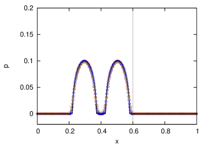
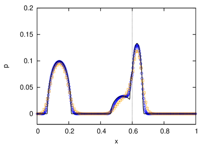
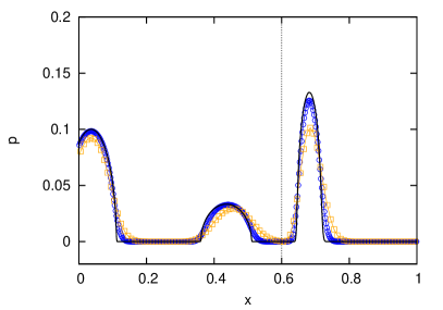
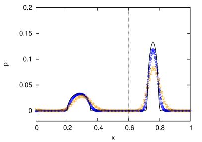
Figure 1: The computed results ($\Delta x=0.01$ (${\color[rgb]{1,0.68,0.36}-\circ-}$) and $\Delta x=0.0025$ (${\color[rgb]{0,0,1}-\circ-}$)) converge to the reference solution (black line) as seen in the snapshots ($t=0.104$ (top-left), $t=0.26$ (top-right), $t=0.364$ (bottom-left) and $t=0.52$ (bottom-right)).

While the augmented scheme converges to the reference solution, it has a higher dispersion error that manifests itself in a phase error of the bumps propagating through the domain. As the mesh resolution is refined, the dispersion error is rapidly reduced. Fig. 2 shows a detail of the small reflected hump at $t=0.52$ for different mesh sizes. It must be noted that the reference wave propagation scheme does not show any dispersion error (i.e., the numerical representation of the bump is symmetric which respect to the center of the exact bump).

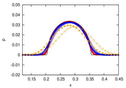
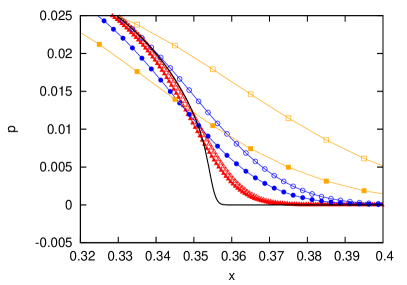
Figure 2: The computed results by the augmented solver ($\Delta x=0.01$ (${\color[rgb]{1,0.68,0.36}-\square-}$), $\Delta x=0.0025$ (${\color[rgb]{0,0,1}-\circ-}$) and $\Delta x=0.00125$ (${\color[rgb]{1,0,0}-\triangle-}$)) and reference solver (filled symbols) show a phase error compared to the reference solution (black line) at $t=0.52$, which rapidly reduces as the grid is refined.

3.2 Hyperbolic heat equation

The 1D heat equation in its original parabolic form reads

$$c\left(x\right)\rho\left(x\right)\frac{\partial u}{\partial t}+\frac{\partial}{\partial x}\left(-k\left(x\right)\frac{\partial u}{\partial x}\right)=\phi,$$ (68)

where $u$ is the temperature, $c$ is the specific heat capacity, $\rho$ is the density, $k$ is the thermal conductivity of the material and $\phi$ is a heat source. The equation can be hyperbolized using Cattaneo’s relaxation approach [4] as

$$\left\{\begin{aligned} c\left(x\right)\rho\left(x\right)\frac{\partial u}{\partial t}+\frac{\partial q}{\partial x}=\phi,\\ \varepsilon\frac{\partial q}{\partial t}+k\left(x\right)\frac{\partial u}{\partial x}=-q.\end{aligned}\right.$$ (69)

Here, we introduce $\varepsilon$ as the relaxation time, and $q$ as the flow of heat energy per unit area. For $\varepsilon\rightarrow 0$, the hyperbolic form in Eq. (69) converges to the original form in Eq. (68). See B for the eigenvalues and eigenvectors of the system.

Proposition 3.1

For a given cell size $\Delta x$ and a first order accurate numerical solver, the value of $\varepsilon$ can be constrained as

$$\left\{\begin{aligned} \varepsilon<\frac{O\left(1\right)\Delta x}{K_{1}},\\ K_{1}=\frac{1-2^{-\frac{1}{2}}}{2^{\frac{1}{2}}-1}.\end{aligned}\right.$$ (70)

Here, $O\left(1\right)$ denotes the error of a first order numerical scheme.

Proof 3.1

Omitted here. See [17] for a detailed proof.

Proposition 3.2

Let $f:\,\mathbb{R}\rightarrow\mathbb{R}$ be a function with compact support on a domain $\Omega$ that satisfies $\frac{\partial f\left(x\right)}{\partial x}=\mathscr{M}f^{-1}\left(x\right)$, with $f^{-1}:\mathbb{R}\rightarrow\mathbb{R}$, and $f\left(x\right)f^{-1}\left(x\right)=1$. Then, if $\phi=0$, $c\left(x\right)=\rho\left(x\right)=1$, and $k\left(x\right)=f$, then $f$ is a steady state solution of Eq. (68) as well as Eq. (69).

Proof 3.2

Since

$$\frac{\partial u}{\partial x}=\mathscr{M}f^{-1},$$ (71)

we obtain

$$q=-k\left(x\right)\frac{\partial u}{\partial x}=-\mathscr{M},$$ (72)

which yields a zero flux in the first equation of the system in Eq. (68) and Eq. (69). Hence, $u$ does not change in time and Prop. 3.2 is thus proved.

Corollary 3.2.1

Consider Eq. (69) in an infinite 1D domain. If $\phi=0$ and $k\left(x\right)=\frac{\mathscr{M}}{\mathscr{W}\text{sin}\left(x\right)+\mathscr{C}}$, then $u\left(x\right)=-\mathscr{W}\text{cos}\left(x\right)+\mathscr{C}x$ is a steady state solution of the system for $\forall{\left(\mathscr{M},\mathscr{W},\mathscr{C}\right)}\in\mathbb{R}:|\mathscr{C}|>|\mathscr{W}|$.

Corollary 3.2.2

Consider Eq. (69) in the domain $\Omega=[a,b]$. Let $\phi=0$ and

$$k\left(x\right)=\begin{cases}k_{1}&\text{if }x\leq\frac{b+a}{2}-\frac{\delta}{2},\\ \tilde{k}&\text{if }\frac{b+a}{2}-\frac{\delta}{2}<x<\frac{b+a}{2}+\frac{\delta}{2},\\ k_{2}&\text{if }x\geq\frac{b+a}{2}+\frac{\delta}{2},\end{cases}$$ (73)

with $k_{1},k_{2}\in\mathbb{R}$ being nonzero constant conductivities, $\tilde{k}=(k_{1}+k_{2})/2$ and $\delta\in\mathbb{R}$ being the conductivity and the thickness of the transition layer. Then $q\left(x\right)=\mathscr{M}$ and

$$u(x)=\begin{cases}-\frac{\mathscr{M}}{k_{2}}x&\text{if }x\leq\frac{b+a}{2}-\frac{\delta}{2},\\ -\mathscr{M}\left(\frac{1}{k_{1}}x+\frac{k_{1}-k_{2}}{k_{1}k_{2}}x^{*}+\frac{1}{k_{1}}\delta-\frac{2}{\tilde{k}}\delta\right)&\text{if }x\geq\frac{b+a}{2}+\frac{\delta}{2},\\ \end{cases}$$ (74)

with $x^{*}=\frac{b+a}{2}-\frac{\delta}{2}$ is a weak solution of Eq. (69) at the steady state, provided that a linear averaging of the coefficient matrix in Eq. (69) is used.

Corollary 3.2.3

In the limit when $\delta\rightarrow 0$, the expressions in Cor. 3.2.2 represents the solution of a pure discontinuous transition in the medium properties (e.g., the conductivity). Such solution reads $q\left(x\right)=\mathscr{M}$ and

$$u\left(x\right)=\begin{cases}-\frac{\mathscr{M}}{k_{2}}x&\text{if }x\leq\frac{b+a}{2},\\ -\mathscr{M}\left(\frac{1}{k_{1}}x+\left(\frac{k_{1}-k_{2}}{k_{1}k_{2}}\right)\left(\frac{b+a}{2}\right)\right)&\text{if }x\geq\frac{b+a}{2}.\\ \end{cases}$$ (75)

Corollary 3.2.4

When considering the numerical resolution of Eq. (69) by means of an augmented scheme and $\delta=\Delta x$, then the solution in Cor. 3.2.2 corresponds to the numerical solution provided by the scheme under steady state. This means that, in the case of a pure discontinuous transition, the numerical scheme will artificially enforce the presence of a transition layer of size $\delta=\Delta x$. As the grid is refined, the size of the transition layer is reduced and tends to zero, thus approaching the exact solution of the pure discontinuous transition.

Proposition 3.3

Consider Eq. (69) in the domain $\Omega=[a,b]$. If $\phi,k\in\mathbb{R}$ are nonzero constants, then $q\left(x\right)=q(a)+\phi(x-a)$ and $u\left(x\right)=u(a)-\frac{q(a)}{k}(x-a)-\frac{\phi}{2k}(x-a)^{2}$ is a steady solution of Eq. (69), with $q(a)$ the heat flux at the inlet and $u(a)$ the temperature at the inlet.

Proof 3.3

The given expressions for the discharge and temperature in Prop. 3.3 satisfy the system in Eq. (69), namely the equations

$$\left\{\begin{aligned} &\frac{\partial q}{\partial x}=\phi,\\ &k\frac{\partial u}{\partial x}=-q.\end{aligned}\right.$$ (76)

Prop. 3.3 is thus proved.

In the following, we show results obtained by the augmented solver for the hyperbolic heat equation at the steady state. For contrast, we compute results with a deliberately not well-balanced wave propagation scheme, which uses a centered integration of the source term.

We note that high-order accurate steady state solutions can be computed using wave propagation algorithms (e.g., by following the approaches in [12] (fractional time stepping) and [15] (path-conservative approach)). The presented results are for illustration purposes only, and do not represent the state of the art wave propagation solvers.

3.2.1 Steady solution considering a constant conductivity

This case is devoted to the resolution of the hyperbolized heat equation with $\rho\left(x\right)=c\left(x\right)=1$ and $\phi=0$, on the domain $x\in[a,b]$, where $a=0$ and $b=10$. The conductivity, $k\left(x\right)$, is set constant. Following Cor. 3.2.1, we impose $\mathscr{M}=1$, $\mathscr{W}=0$ and $\mathscr{C}=2$. Initial conditions for $u$ and $q$ are applied following Cor. 3.2.1. Fixed Dirichlet boundary conditions are applied for both heat flux and temperature. The heat flux is set upstream and the temperature downstream, as

$$q_{in}=-1,\quad u_{out}=\mathscr{C}b.$$ (77)

The augmented solver reproduces the exact solution independent of the grid resolution. Both the nonconservative products and the source term are constant, and the linear approximation of the integral of these terms is exact, see Prop. 2.1. The not well-balanced scheme is not able to reproduce the analytical reference solution, neither for the temperature nor the heat flux. See Fig. 3, which shows the computed solution of both schemes after $30,000$ time steps, using a CFL number of $0.8$. The $L_{\infty}$-norm of the error of the augmented scheme is in the range of machine accuracy, see Tab. 1.

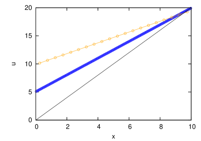
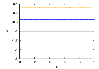
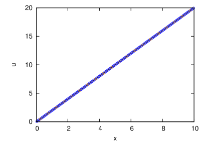
Figure 3: Constant conductivity: The not well-balanced scheme (top) fails to reproduce the reference solution at the steady state (black line), but the augmented scheme (bottom) accurately reproduces it. (Numerical solution computed using $\Delta x=0.5$ (${\color[rgb]{1,0.68,0.36}-\circ-}$) and $\Delta x=0.05$ (${\color[rgb]{0,0.0,1}-\circ-}$)).

	Unbalanced		Augmented
Mesh	$L_{\infty}(u)$	$L_{\infty}(q)$	$L_{\infty}(u)$	$L_{\infty}(q)$
$\Delta x=0.5$	9.65e+00	5.21e-01	2.22e-16	3.33e-16
$\Delta x=0.05$	5.05e+00	2.56e-01	8.88e-16	1.38e-14

Table 1: Constant conductivity: $L_{\infty}$ error norms for the numerical solution computed by the not well-balanced algorithm and the augmented scheme.

3.2.2 Steady solution considering a smoothly varying conductivity

This case considers again the resolution of the hyperbolized homogeneous heat equation (i.e., $\phi=0$) with $\rho\left(x\right)=c\left(x\right)=1$, but in this case a varying conductivity is chosen. $k\left(x\right)$ is set as presented in Cor. 3.2.1, with $\mathscr{M}=1$, $\mathscr{W}=1.8$ and $\mathscr{C}=2$. The computational domain is given by $x\in[a,b]$, where $a=0$ and $b=10$. Initial conditions for $u$ and $q$ are applied following Prop. 3.2.1. Fixed Dirichlet boundary conditions are applied for both heat flux and temperature. The heat flux is set upstream and the temperature downstream, as follows

$$q_{in}=-1,\quad u_{out}=-\mathscr{W}\mathrm{cos}\left(b\right)+\mathscr{C}b$$ (78)

Using a CFL number of $0.8$, steady state is reached after $500,000$ time steps. The augmented solver accurately reproduces the reference solution for heat flux independent of grid resolution (as anticipated in Cor. 2.1.1), but is unable to reproduce the reference solution for the temperature. This is due to the temperature and conductivity being sinusoidal functions that do not satisfy the condition in Prop. 2.1, see the $L_{\infty}$-norms for the errors in Tab. 2. Despite this fact, the augmented scheme is more accurate than the not well-balanced scheme in recovering the steady state solution, see Fig. 4.

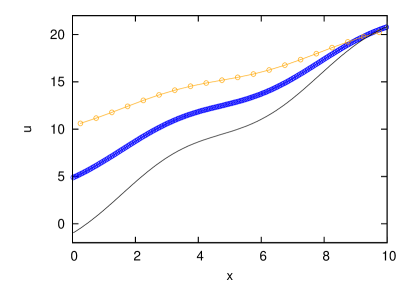
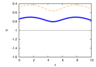
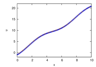
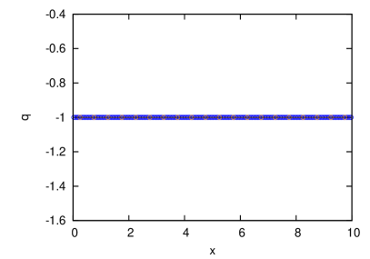
Figure 4: Smoothly varying conductivity: The not well-balanced scheme (top) fails to reproduce the reference solution at the steady state (black line), the augmented scheme (bottom) reproduces it more accurately. (Numerical solution computed using $\Delta x=0.5$ (${\color[rgb]{1,0.68,0.36}-\circ-}$) and $\Delta x=0.05$ (${\color[rgb]{0,0.0,1}-\circ-}$)).

	Unbalanced		Augmented
Mesh	$L_{\infty}(u)$	$L_{\infty}(q)$	$L_{\infty}(u)$	$L_{\infty}(q)$
$\Delta x=0.5$	1.11e+01	5.71e-01	1.86e-01	5.66e-14
$\Delta x=0.05$	5.85e+00	2.96e-01	2.02e-03	7.56e-14

Table 2: Smoothly varying conductivity: $L_{\infty}$ error norms for the numerical solution computed by the not well-balanced algorithm and the augmented scheme.

3.2.3 Steady solution considering a piecewise constant conductivity

In this case, the hyperbolized heat equation with $\phi=0$, $\rho\left(x\right)=c\left(x\right)=1$ is solved considering a piecewise constant conductivity, given by two constant values of conductivity separated by a discontinuity as

$$k\left(x\right)=\begin{cases}k_{1}=1&\text{if }x<\frac{b+a}{2},\\ k_{2}=4&\text{if }x>\frac{b+a}{2}.\\ \end{cases}$$ (79)

This test case represents the limit situation when making $\delta\rightarrow 0$ in the exact solution of Cor. 3.2.2. The computational domain is given by $x\in[a,b]$, where $a=0$ and $b=10$. Fixed Dirichlet boundary conditions are applied for both heat flux and temperature. The heat flux is set upstream and the temperature downstream as

$$q_{in}=-\mathscr{M},\quad u_{out}=-\frac{\mathscr{M}}{k_{2}}b$$ (80)

where $\mathscr{M}=1$.

Steady state is obtained after $30,000$ time steps with a CFL number of $0.8$. The equilibrium solution provided by the augmented scheme converges to the solution in Cor. 3.2.2, where $\delta=\Delta x$, and converges with first order accuracy to the exact analytical solution in Cor. 3.2.3 as the grid resolution is refined, as stated in Cor. 3.2.4, see the solution plot in Fig. 5 and the detail plot of the domain around the conductivity jump in Fig. 6. The $L_{\infty}$ error norm with respect to the exact solution and the analytical discrete equilibrium solution shows that the model converges to the equilibrium solution with machine accuracy, but not to the exact analytical solution, see Tab. 3.

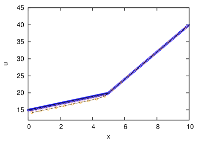
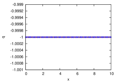
Figure 5: Piecewise constant conductivity: The augmented scheme ($\Delta x=0.5$ (${\color[rgb]{1,0.68,0.36}-\circ-}$), $\Delta x=0.2$ (${\color[rgb]{0.75,0,1}-\circ-}$), $\Delta x=0.05$ (${\color[rgb]{0,0.0,1}-\circ-}$)) converges to the equilibrium solution (dashed line) with machine accuracy, but fails to reproduce the analytical solution (solid black line).

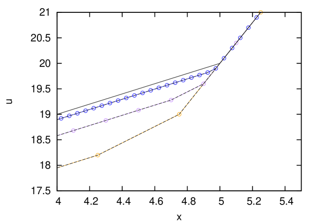
Figure 6: Piecewise constant conductivity: Detail of the solution for temperature, computed by the augmented scheme ($\Delta x=0.5$ (${\color[rgb]{1,0.68,0.36}-\circ-}$), $\Delta x=0.2$ (${\color[rgb]{0.75,0,1}-\circ-}$), $\Delta x=0.05$ (${\color[rgb]{0,0.0,1}-\circ-}$)) shows the deviation between model results and the exact analytical solution (black solid line). The equilibrium solution (dashed line) is always captured with machine accuracy.

	Exact ($\delta=0$)		Equilibrium ($\delta=\Delta x$)
Mesh	$L_{\infty}(u)$	$L_{\infty}(q)$	$L_{\infty}(u)$	$L_{\infty}(q)$
$\Delta x=0.5$	1.05e+00	4.44e-16	1.00e-16	4.44e-16
$\Delta x=0.2$	4.20e-01	5.11e-15	1.78e-15	5.11e-15
$\Delta x=0.05$	1.05e-01	1.58e-14	1.78e-15	1.58e-14

Table 3: Piecewise constant conductivity: $L_{\infty}$ error norms of the numerical solution with respect to the exact solution and the equilibrium solutions computed by the augmented scheme.

3.2.4 Steady solution considering an external heat source

The hyperbolized heat equation with a constant heat source $\phi=0.5$ is considered inside the computational domain $x\in[a,b]$, where $a=0$ and $b=10$. The product of density and specific heat capacity is set to $\rho\left(x\right)c\left(x\right)=0.5$. The conductivity is set constant, $k\left(x\right)=3$, yielding to the solution provided in Prop. 3.3, where the discharge at the inlet is set as $q(a)=-1$. Initial conditions for $u$ and $q$ are applied following such solution in Prop. 3.3. Fixed Dirichlet boundary conditions are applied for both heat flux and temperature. The heat flux is set upstream and the temperature downstream, as follows

$$q_{in}\equiv q(a)=-1,\quad u_{out}=-\frac{\phi}{2k}b^{2}-q(a)\frac{b}{k}$$ (81)

Steady state is obtained after $500,000$ time steps, using a CFL number of $0.9$. As anticipated in Cor. 2.1.1, the augmented scheme provides the exact solution independent of the grid, ensuring the equality in Eq. (12), see Fig. 7, and Tab. 2.

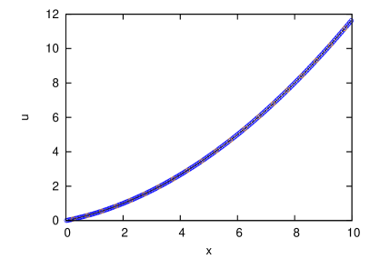
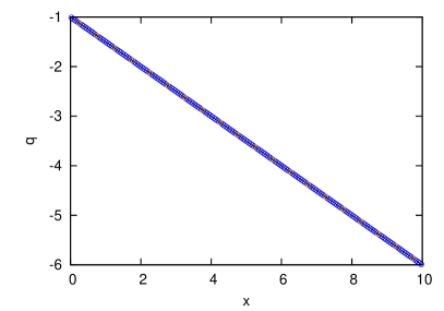
Figure 7: External heat source: Augmented scheme ($\Delta x=0.5$ (${\color[rgb]{1,0.68,0.36}-\circ-}$) and $\Delta x=0.05$ (${\color[rgb]{0,0.0,1}-\circ-}$)) converges to the exact solution (solid line) with machine accuracy.

Mesh	$L_{\infty}(u)$	$L_{\infty}(q)$
$\Delta x=0.5$	1.00e-16	4.44e-16
$\Delta x=0.05$	3.55e-15	1.33e-14

Table 4: External heat source: $L_{\infty}$ error norms for the numerical solution computed by the augmented scheme.

3.2.5 Transient solution for a Riemann problem with constant conductivity

This test considers the resolution of a RP for the hyperbolic heat equation in Eq. (69) with the IC given as

$$\left\{\begin{aligned} &\accentset{\circ}{u}\left(x\right)=\begin{cases}-1&\text{if }x<5,\\ 1&\text{if }x>5,\\ \end{cases}\\ &\accentset{\circ}{q}\left(x\right)=0,\end{aligned}\right.$$ (82)

and considering a constant conductivity $k(x)=0.05$. No source term is considered, $\phi=0$, and $\rho\left(x\right)=c\left(x\right)=1$. The computational domain is set as $\Omega=[0,10]$ and the solution is computed at $t=2$ and $t=5$ using $\Delta x=0.5$ and $\Delta x=0.1$ by means of the augmented scheme. The CFL number is set to 0.5 and $\varepsilon$ is set according to Prop. 3.1.

For this problem configuration it is possible to find an analytical condition, which reads:

$$u(x,t)=\text{erf}\left(\frac{x-5}{2\sqrt{kt}}\right)\,,\quad q(x,t)=-k\frac{e^{-(x-5)^{2}/(4kt))}}{\sqrt{k\pi t}};$$ (83)

The numerical results evidence that the augmented scheme accurately captures the transient evolution of the temperature and heat flux and converges to the exact solution when the mesh is refined. The numerical solution is depicted in Fig. 8.

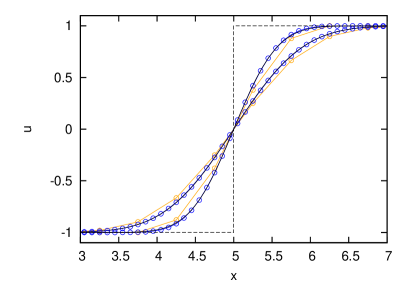
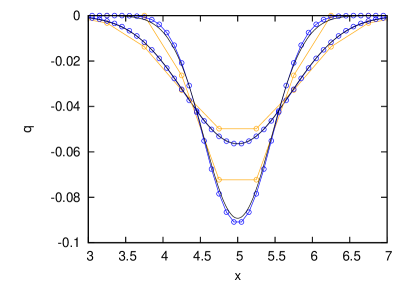
Figure 8: RP with constant conductivity: Numerical solution provided by the augmented scheme ($\Delta x=0.5$ (${\color[rgb]{1,0.68,0.36}-\circ-}$) and $\Delta x=0.1$ (${\color[rgb]{0,0.0,1}-\circ-}$)) accurately captures the exact solution (solid line) in the transient case. Dashed line shows the IC.

3.2.6 Transient solution for a Riemann problem with piecewise constant conductivity

This test considers the resolution of a RP for the heat equation in Eq. (68) with the initial condition in Eq. (82). No source term is considered (i.e., $\phi=0$). Medium properties are set to $\rho\left(x\right)=c\left(x\right)=1$. Two different piecewise constant distributions of conductivity are considered. The first case, referred to as RP-a, uses

$$k(x)=\begin{cases}0.1&\text{if }x<5,\\ 0.01&\text{if }x>5,\end{cases}$$ (84)

whereas the second case, referred to as RP-b, uses

$$k(x)=\begin{cases}0.1&\text{if }x<5,\\ 0.05&\text{if }x>5.\end{cases}$$ (85)

The computational domain is set as $\Omega=[0,10]$ and the solution is computed at $t=8$ using $\Delta x=0.5$ and $\Delta x=0.1$ by means of the augmented scheme. The CFL number is set to 0.5 and $\varepsilon$ is set following Prop. 3.1.

A numerical solution computed with the augmented scheme on a grid of $\Delta x=0.001$ is used as reference solution for this case. The numerical results evidence that the augmented scheme converges to the reference solution when the mesh is refined. The proposed scheme is able to handle strong discontinuities of the conductivity coefficient without generating spurious oscillations. The numerical solution for these test cases is depicted in Fig. 9 and Fig. 10.

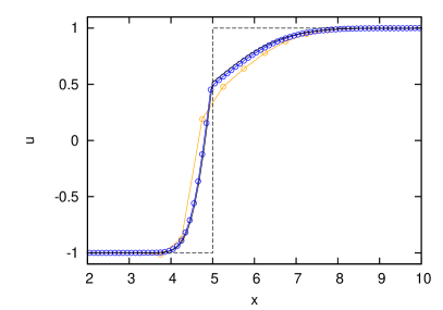
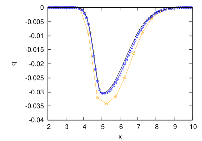
Figure 9: RP-a with conductivity jump: Numerical solution provided by the augmented scheme ($\Delta x=0.5$ (${\color[rgb]{1,0.68,0.36}-\circ-}$) and $\Delta x=0.1$ (${\color[rgb]{0,0.0,1}-\circ-}$)) converges to the reference solution (solid line). Dashed line shows the IC.

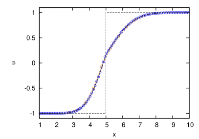
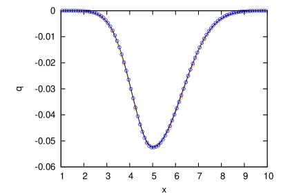
Figure 10: RP-b with conductivity jump: Numerical solution provided by the augmented scheme ($\Delta x=0.5$ (${\color[rgb]{1,0.68,0.36}-\circ-}$) and $\Delta x=0.1$ (${\color[rgb]{0,0.0,1}-\circ-}$)) converges to the reference solution (solid line). Dashed line shows the IC.

4 Conclusions

This paper proposes a general framework to well-balance linear nonconservative hyperbolic systems with source terms, focusing on the equilibrium properties of the numerical schemes. Our schemes are based on augmented Riemann solvers, which are revisited here using a common framework that uses a geometric reinterpretation of source terms. This geometric reinterpretation allows to handle arbitrary sources in the same manner (i.e., they are introduced in the definition of the Riemann problem as a singular source term).

It is proved that the schemes constructed within the proposed framework are intrinsically well-balanced under linearity conditions. In the problems where the source terms are linear and the solution yields linear nonconservative products, the schemes will reproduce the exact solution with machine precision. Otherwise, they will converge to the exact solution with the order of accuracy chosen for the discretization (e.g., first order in this work). It must be noted that the schemes could be extended to higher order of accuracy using traditional TVD, ENO or WENO reconstructions in space [10, 16] and Runge-Kutta or ADER time-stepping [27, 24, 20, 7].

In the presented test cases, we show that the proposed methods accurately capture the transient evolution of the waves, though they involve a higher dispersion error than the traditional wave propagation algorithm [14]. The hyperbolized heat equation allows a very complete exercise of the equilibrium properties of the proposed methods under a wide variety of conditions (e.g., spatial variation of the medium conductivity, presence of a heat source term with a possible variation in space, and presence of discontinuities). The proposed methods have been validated using as benchmark a complete set of test cases, involving transient and steady solutions, for which the analytical solutions have been presented. The numerical results evidence that the proposed scheme is able to provide a time-accurate resolution of transient cases. For steady-state problems, the schemes reproduce the exact discharge with machine accuracy for all cases provided a constant or linear heat source term. The temperature is generally approximated with first order of accuracy. In the case when the system in Eq. (1) satisfies linearity conditions, the scheme also reproduces the exact temperature with machine accuracy.

The schemes also evidence a good performance (i.e., convergence with mesh refinement $L_{\infty}=\mathcal{O}(\Delta x)$), when dealing with discontinuities in the medium properties. The generation of an artificial transition layer in the numerical solution, in the sense of the 3-shock representation of discontinuous solutions in nonlinear systems [21] is observed. The size of such transition layer and the value of the variables in it have been analytically derived and numerically confirmed for the hyperbolized heat equation.

The proposed approach is a reliable tool to provide an accurate numerical solution to heat diffusion problems in heterogeneous media in presence of different source terms. In presence of heat sources, it allows to exactly (or accurately, if the source function is nonlinear and has to be numerically approximated) preserve the balance of heat fluxes. These properties make the proposed schemes a useful tool for realistic engineering problems such as the simulation of phase-change problems, refer to [28, 25, 26, among others], and may represent an alternative to more traditional schemes such as the finite difference methods for instance.

The methods in this work can be easily extended to solve convection-diffusion problems where the nonconservative products coexist with the conservative contributions that arise from the convective term. An exact balancing of those terms can be achieved in the same way. The extension of the proposed methods to higher spatial dimensions is straightforward following a dimensional splitting approach.

Appendix A Eigenanalysis of the linear acoustic equation

The linear acoustic equation in Eq. 65 can be written in the form of Eq. 1 with

$$U=\left[\begin{array}[]{c}p\\ u\end{array}\right],\;\mathcal{A}=\left[\begin{array}[]{c c}0&K\\ \frac{1}{\rho}&0\end{array}\right],\;S=\left[\begin{array}[]{c}0\\ 0\end{array}\right].$$ (86)

The eigenvalues of the coefficient matrix $\mathcal{A}$ read

$$\lambda^{1}=-\sqrt{\frac{K}{\rho}},\;\lambda^{2}=\sqrt{\frac{K}{\rho}},$$ (87)

with corresponding right eigenvalue matrix $\mathcal{P}$, and its inverse as

$$\mathcal{P}=\left[\begin{array}[]{c c}-\frac{1}{\sqrt{K/\rho}}&\frac{1}{\sqrt{K/\rho}}\\ 1&1\end{array}\right],\quad\mathcal{P}^{-1}=\frac{1}{2}\left[\begin{array}[]{c c}-\sqrt{\frac{K}{\rho}}&1\\ \sqrt{\frac{K}{\rho}}&1\end{array}\right].$$ (88)

The system is strictly hyperbolic with $2$ real and distinct eigenvalues.

Appendix B Eigenanalysis of the hyperbolic heat equation

B.1 Original hyperbolic heat equation

The hyperbolic heat equation in Eq. 69 can be written in the form of Eq. 1 with

$$U=\left[\begin{array}[]{c}u\\ q\end{array}\right],\;\mathcal{A}=\left[\begin{array}[]{c c}0&r\\ \frac{k}{\varepsilon}&0\end{array}\right],\;S=\left[\begin{array}[]{c}r\phi\\ -\frac{q}{\varepsilon}\end{array}\right],$$ (89)

and $c\left(x\right)\rho\left(x\right)=1/r$ for simplicity. The eigenvalues of the coefficient matrix $\mathcal{A}$ read

$$\lambda^{1}=-\sqrt{\frac{kr}{\varepsilon}},\;\lambda^{2}=\sqrt{\frac{kr}{\varepsilon}},$$ (90)

with corresponding right eigenvalue matrix $\mathcal{P}$, and its inverse as

$$\mathcal{P}=\left[\begin{array}[]{c c}-\sqrt{\frac{\varepsilon r}{k}}&\sqrt{\frac{\varepsilon r}{k}}\\ 1&1\end{array}\right],\quad\mathcal{P}^{-1}=\frac{1}{2}\left[\begin{array}[]{c c}-\sqrt{\frac{k}{\varepsilon r}}&1\\ \sqrt{\frac{k}{\varepsilon r}}&1\end{array}\right].$$ (91)

The system is strictly hyperbolic with $2$ real and distinct eigenvalues.

B.2 Augmented conservative hyperbolic heat equation

According to the augmented scheme formulation in flux form in Sec. 2.2.2, the convective part of the system of equations in Eq. 69 can be rewritten in conservative form (see Eq. (44)), yielding

$$\left\{\begin{aligned} &\frac{\partial u}{\partial t}+r\frac{\partial q}{\partial x}=r\phi,\\ &\frac{\partial q}{\partial t}+\frac{1}{\varepsilon}\frac{\partial(ku)}{\partial x}=\frac{u}{\varepsilon}\frac{\partial k}{\partial x}-\frac{q}{\varepsilon}.\end{aligned}\right.$$ (92)

This system can be written in matrix form as in Eq. 44 with

$$\bar{U}=\left[\begin{array}[]{c}u\\ q\\ k\end{array}\right],\;\bar{F}=\left[\begin{array}[]{c}q\\ \frac{ku}{\varepsilon}\\ 0\end{array}\right],\;\bar{\mathcal{K}}=\left[\begin{array}[]{c c c}0&0&0\\ 0&0&\frac{u}{\varepsilon}\\ 0&0&0\end{array}\right],\;S=\left[\begin{array}[]{c}r\phi\\ -\frac{q}{\varepsilon}\\ 0\end{array}\right].$$ (93)

For the system in Eq. (44), it is possible to define a Jacobian matrix of the flux $\bar{F}$ (see Eq. (46))

$$\bar{\mathcal{M}}=\left[\begin{array}[]{c c c}0&r&0\\ \frac{k}{\varepsilon}&0&\frac{u}{\varepsilon}\\ 0&0&0\end{array}\right],$$ (94)

The eigenvalues of the coefficient matrix $\bar{\mathcal{M}}$ read

$$\lambda^{1}=-\sqrt{\frac{kr}{\varepsilon}},\quad\lambda^{2}=0,\quad\lambda^{3}=\sqrt{\frac{kr}{\varepsilon}},$$ (95)

with corresponding right eigenvalue matrix $\mathcal{P}$, and its inverse as

$$\bar{\mathcal{P}}=\left[\begin{array}[]{c c c}-\sqrt{\frac{\varepsilon r}{k}}&{\frac{u}{k}}&\sqrt{\frac{\varepsilon r}{k}}\\ 1&0&1\\ 0&1&0\\ \end{array}\right],\quad\bar{\mathcal{P}}^{-1}=\frac{1}{2}\left[\begin{array}[]{c c c}-\sqrt{\frac{k}{\varepsilon r}}&1&-\frac{u}{\sqrt{\varepsilon kr}}\\ 0&0&2\\ \sqrt{\frac{k}{\varepsilon r}}&1&\frac{u}{\sqrt{\varepsilon kr}}\end{array}\right].$$ (96)

The system is strictly hyperbolic with $3$ real and distinct eigenvalues.

References

- [1] E. Audusse, F. Bouchut, M. O. Bristeau, R. Klein, and B. Perthame. A fast and stable well-balanced scheme with hydrostatic reconstruction for shallow water flows. SIAM Journal on Scientific Computing, 25:2050–2065, 2004.
- [2] A. Bermudez and M. Vazquez. Upwind methods for hyperbolic conservation laws with source terms. Computers and Fluids, 23:1049–1071, 1994.
- [3] F. Bouchut, J. Le Sommer, and V. Zeitlin. Frontal geostrophic adjustment and nonlinear wave phenomena in one-dimensional rotating shallow water. Part 2. High-resolution numerical simulations. Journal of Fluid Mechanics, 514:35–63, 2004.
- [4] C. Cattaneo. Sur une forme d’équation de la chaleur éliminant le paradoxe d’une propagation instantanée. Comptes Rendus de l’Académie des Sciences, 247:431–433, 1958.
- [5] R. Courant, K. Friedrichs, and H. Lewy. Über die partiellen Differenzengleichungen der mathematischen Physik. Mathematische Annalen, 100:32–74, 1928.
- [6] Michael Dumbser and Eleuterio F. Toro. A simple extension of the Osher Riemann solver to non-conservative hyperbolic systems. Journal of Scientific Computing, pages 70–88, 2011.
- [7] Michael Dumbser, Olindo Zanotti, Arturo Hidalgo, and Dinshaw S. Balsara. ADER-WENO finite volume schemes with space–time adaptive mesh refinement. Journal of Computational Physics, 248:257 – 286, 2013.
- [8] Edwige Godlewski and Pierre-Arnaud Raviart. Numerical Approximation of Hyperbolic Systems of Conservation Laws. Springer-Verlag, New York, USA, 1996.
- [9] S. K. Godunov. A difference scheme for numerical solution of discontinuous solution of hydrodynamic equations. Matematicheskii Sbornik, 47:271–306, 1959.
- [10] Ami Harten, Bjorn Engquist, Stanley Osher, and Sukumar R Chakravarthy. Uniformly high order accurate essentially non-oscillatory schemes, III. Journal of Computational Physics, 71:231–303, 1987.
- [11] E. V. Haynsworth. On the Schur Complement. Basel Mathematical Notes, #BNB 20, Basel, Switzerland, 1968.
- [12] R. J. LeVeque. Intermediate boundary conditions for time-split methods applied to hyperbolic partial differential equations. Mathematics of Computation, 47:37–54, 1986.
- [13] R. J. LeVeque. Finite Volume Methods for Hyperbolic Problems. Cambridge University Press, New York, USA, 2002.
- [14] Randall J. LeVeque. Wave propagation algorithms for multidimensional hyperbolic systems. Journal of Computational Physics, 131:327–353, 1997.
- [15] Randall J. LeVeque. A well-balanced path-integral f-wave method for hyperbolic problems with source terms. Journal of Scientific Computing, 48:209–226, 2011.
- [16] Xu-Dong Liu, Stanley Osher, and Tony Chan. Weighted essentially non-oscillatory schemes. Journal of Computational Physics, 115:200–212, 1994.
- [17] G. I. Montecinos, L. O. Müller, and E. F. Toro. Hyperbolic reformulation of a 1D viscoelastic blood flow model and ADER finite volume schemes. Journal of Computational Physics, 266:101–123, 2014.
- [18] J. Murillo and P. García-Navarro. Improved Riemann solvers for complex transport in two-dimensional unsteady shallow flow. Journal of Computational Physics, 230:7202–7239, 2011.
- [19] Javier Murillo and Adrián Navas-Montilla. A comprehensive explanation and exercise of the source terms in hyperbolic systems using roe type solutions. Application to the 1D-2D shallow water equations. Advances in Water Resources, 98:70–96, 2016.
- [20] A. Navas-Montilla and J. Murillo. Asymptotically and exactly energy balanced augmented flux-ader schemes with application to hyperbolic conservation laws with geometric source terms. Journal of Computational Physics, 317:108–147, 2016.
- [21] A. Navas-Montilla and J. Murillo. Improved Riemann solvers for an accurate resolution of 1D and 2D shock profiles with application to hydraulic jumps. Journal of Computational Physics, 378:445–476, 2019.
- [22] C. Parés and M. Castro. On the well-balance property of Roe’s method for nonconservative hyperbolic systems. Applications to shallow-water systems. ESAIM: Mathematical Modelling and Numerical Analysis, 38:821–852, 2004.
- [23] P. L. Roe. Approximate Riemann solvers, parameter vectors and difference schemes. Journal of Computational Physics, 43:357–372, 1981.
- [24] T. Schwartzkopff, C. D. Munz, and E. F. Toro. ADER: A high-order approach for linear hyperbolic systems in 2D. Journal of Scientific Computing, 17:231–240, 2002.
- [25] V. Shatikian, G. Ziskind, and R. Letan. Numerical investigation of a PCM-based heat sink with internal fins. International Journal of Heat and Mass Transfer, 48:3689–3706, 2005.
- [26] V. Shatikian, G. Ziskind, and R. Letan. Numerical investigation of a PCM-based heat sink with internal fins: Constant heat flux. International Journal of Heat and Mass Transfer, 51:1488–1493, 2008.
- [27] Chi-Wang Shu. Essentially non-oscillatory and weighted essentially non-oscillatory schemes for hyperbolic conservation laws. In Alfio Quarteroni, editor, Advanced Numerical Approximation of Nonlinear Hyperbolic Equations: Lectures given at the 2nd Session of the Centro Internazionale Matematico Estivo (C.I.M.E.) held in Cetraro, Italy, June 23–28, 1997, pages 325–432. Springer Berlin Heidelberg, 1998.
- [28] V. R. Voller and C. Prakash. A fixed grid numerical modelling methodology for convection-diffusion mushy region phase-change problems. International Journal of Heat and Mass Transfer, 30:1709–1719, 1987.
- [29] X. Xia and Q. Liang. A new depth-averaged model for flow-like landslides over complex terrains with curvatures and steep slopes. Engineering Geology, 234:174–191, 2018.