Dissipative coupling, dispersive coupling and its combination
in simplest opto-mechanical systems

Abstract

We apply strategy of variational measurement to simplest variant of dissipative coupling (test mass displacement change transitivity of a single mirror) and compare it with simplest dispersive coupling (a single mirror as a test mass, which position changes the phase of reflected wave). We compare a ponderomotive squeezing in this two kinds of coupling. Also we analyze simplest variant of combined coupling, in which both dissipative and dispersive couplings are used, and show that it creates stable optical rigidity even in case of single pump. We demonstrate that variational measurement can be applied for combined coupling.

I Introduction

Interaction of light in an optical cavity and a mechanical oscillator or a free mass is a subject of opto-mechanics Aspelmeyer et al. (2014). The simple realization of so called dispersive opto-mechanic coupling is based on cavity in which a position of a mechanical body (movable mirror) changes eigen frequency of cavity and at the same time light pressure experiences a force proportional to optical power or number of optical quanta circulating in the optical cavity. Opto-mechanical systems having several degrees of freedom provide possibility of more complex interactions ranging from radiation puling (negative radiation pressure) Povinelli et al. (2005); Maslov et al. (2013), opto-mechanical interaction proportional to the quadrature of electromagnetic field S.P. Vyatchanin and A.B. Matsko (1993, 1996); A.B. Matsko and S.P. Vyatchanin (1997); H.J. Kimble et al. (2001) to the interaction depending on test mass speed (not the coordinate) of the mechanical system V.B. Braginsky and F.Ya. Khalili. (1990); V.B. Braginsky et al. (2000).

Opto-mechanics are very important in precision measurements using transduction mechanism between the mechanical and optical degrees of freedom via enabling various sensors, like gravitational wave detectors LVC-Collaboration (2013); J. Aasi et al et al.(2015) (LIGO Scientific Collaboration); Martynov et al. (2016); Asernese et al. (2015); Dooley et al. (2016); Aso et al. (2013), torque sensors M. Wu et al. (2014), and magnetometers S. Forstner and S. Prams and J. Knittel and E.D. van Ooijen and J.D. Swaim and G.I. Harris and A. Szorkovszky and W.P. Bowen and H. Rubinsztein-Dunlop (2012).

The accuracy of the mechanical position measurement in an opto-mechanical system usually is restricted due to quantum back action by so called standard quantum limit (SQL) V.B. Braginsky (1968); V.B. Braginsky and F.Ya. Khalili (1992). The SQL was studied in many systems ranging from macroscopic kilometre-sized gravitational wave detectors H.J. Kimble et al. (2001) to microcavities Kippenberg and Vahala (2008); J.M. Dobrindt and T.J. Kippenberg (2010). An example of a measurement restricted by SQL is detection of a classical force acting on a mechanical degree of freedom of an opto-mechanical system. However, SQL of force measurement is not a fundamentally unavoidable limit. It can be surpassed using variational measurement S.P. Vyatchanin and A.B. Matsko (1993); Vyatchanin and Zubova (1995); H.J. Kimble et al. (2001), squeezed light usage The LIGO Scientific collaboration (2011); LIGO Scientific Collaboration and Virgo Collaboration (2013); Tse et al. (2019); Asernese et al. (2019); Yap et al. (2020); Yu et al. (2020); Cripe et al. (2019), opto-mechanical velocity measurement V.B. Braginsky and F.Ya. Khalili. (1990); V.B. Braginsky et al. (2000), and measurements in opto-mechanical systems with optical rigidity V.B. Braginsky and F.Ya. Khalili (1999); F.Ya. Khalili (2001).

There are two kinds of opto-mechanic coupling: dispersive and dissipative ones. For dispersive one displacement of mirror changes normal frequency of cavity, whereas for dissipative coupling displacement of test mass changes transparency of input mirror and, hence, relaxation rate of cavity. Dissipative coupling was proposed theoretically F. Elste and S.M. Girvin and A.A. Clerk (2009) and implemented experimentally M. Li and W.H.P. Pernice and H.X. Tang (2009); Weiss et al. (2013); M. Wu et al. (2014); Hryciw et al. (2015) nearly a decade ago. It was studied in a variety of opto-mechanical systems, including Fabry-Perot interferometer M. Li and W.H.P. Pernice and H.X. Tang (2009); Weiss et al. (2013); M. Wu et al. (2014); Hryciw et al. (2015), Michelson-Sagnac interferometer Xuereb et al. (2011); Tarabrin et al. (2013); Sawadsky et al. (2015), and ring resonators S. Huang and G.S. Agarwal (2010a, b). It was shown S.P. Vyatchanin and A.B. Matsko (2016) that an opto-mechanical transducer based on dissipative coupling of optical and mechanical degrees of freedom gives possibility to realize quantum speed meter which, in turn, allows to surpass SQL.

In this paper we analyze dispersive and dissipative coupling in simplest opto-mechanical system without any cavity.

Recall dispersive coupling in cavity is characterized by dependence of normal frequency on position of test mass, for example, for Fabry-Perot cavity it is position of input or end mirror. So, we model dispersive coupling without cavity by movable mirror (it is free test mass), phase of reflected light depends on test mass position.

In turn, dissipative coupling in cavity means that its relaxation rate depends on test mass position, for Fabry Perot cavity it means that transmittance of input mirror depends on test mass position. So we model dissipative coupling without cavity as mirror which amplitude reflectivity $R$ and transmittance $T$ depend on position of test mass. In particular, it corresponds to Michelson-Sagnac interferometer (MSI) Xuereb et al. (2011); Tarabrin et al. (2013); Sawadsky et al. (2015) as a generalized mirror (GM), where test mass is a movable completely reflecting mirror $M$.

We also consider opposite case of movable beam splitter (BS) in MSI and fixed position of mirror $M$ ($x_{m}$ is a constant) — it is a model of mirror with combined (both dispersive and dissipative) couplings.

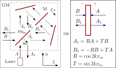
Figure 1: Michelson-Sagnac interferometer in case of fixed position of BS ($y=0$) is a GM which transparency and reflectivity depends on position of test mass (completely reflecting mirror $M$) – example of dissipative coupling. In opposite case of movable BS and fixed position $x_{m}=0$ of mirror $M$ it is a model of mirror with both dispersive and dissipative couplings.

II MSI as a generilized mirror

The detailed analysis of MSI is presented in Appendix A, MSI can be considered as GM with amplitude transmittance $T$ and reflectivity $R$ depending on displacements $x_{m},\ y_{bs}$ (33). Below we present displacements as

$$x_{m} =x_{0}+x,\ y_{bs}=y_{0}+y$$ (1)

where $x_{0},\ y_{0}$ are mean constants (can be chosen) and $x,\ y$ are small variables. Then we can expand $R,\ T$ (33) into series

$$R \simeq R_{0}+T_{0}\,k\big{[}2x+\sqrt{2}\,y\big{]}\,,$$ (2a)

$$T \simeq-T_{0}+R_{0}\,k\big{[}2x+\sqrt{2}\,y\big{]}\,,$$ (2b)

$$R_{0} =\cos k\big{(}2x_{0}+\sqrt{2}\,y_{0}\big{)},\quad T_{0}=-\sin k\big{(}2x_{0}+\sqrt{2}\,y_{0}\big{)},$$

where $k=\omega_{0}/c$, $\omega_{0}$ is a carrier frequency of light waves. Below we put $y_{0}=0$ for simplicity, then only $x_{0}$ defines $T_{0},\ R_{0}$.

Below we present amplitudes of waves as large constant amplitude (denoted capital letter) plus small amplitudes (denoted by the same small letter) containing noise and signal. For example

$$\mathcal{A} =A+\hat{a},\quad\mathcal{A}_{1}=A_{1}+\hat{a}_{1},\quad\text{and so on.}$$ (3)

Input waves are in coherent state so operators $\hat{a},\ \hat{b}$ describe vacuum fluctuation wave, which commutator and correlator are the following

$$\left[\hat{a}(t),\hat{a}^{\dagger}(t^{\prime})\right] =\left[\hat{b}(t),\hat{b}^{\dagger}(t^{\prime})\right]=\delta(t-t^{\prime}),$$ (4)

$$\left\langle\hat{a}(t)\hat{a}^{\dagger}(t^{\prime})\right\rangle =\left\langle\hat{b}(t)\hat{b}^{\dagger}(t^{\prime})\right\rangle=\delta(t-t^{\prime})$$ (5)

Below we use Fourier transform defined as

$$\hat{a}(t) =\int_{-\infty}^{\infty}a(\Omega)\,e^{-i\Omega t}\,\frac{d\Omega}{2\pi}$$ (6)

and by a similar way for others values, denoting Fourier transform by the same letter but without the hat. For Fourier transform of the input fluctuation operators one can derive from (4) and(5):

$$\left[a(\Omega),a^{\dagger}(\Omega^{\prime})\right] =\left[b(\Omega),b^{\dagger}(\Omega^{\prime})\right]=2\pi\,\delta(\Omega-\Omega^{\prime}),$$ (7)

$$\left\langle a(\Omega)a^{\dagger}(\Omega^{\prime})\right\rangle =\left\langle b(\Omega)b^{\dagger}(\Omega^{\prime})\right\rangle=2\pi\,\delta(\Omega-\Omega^{\prime})$$ (8)

III Simplest dissipative couplings

Let consider particular case when BS position is fixed ($y_{0}=0,\ y=0$), then MSI is GM as a model of dissipative coupling Xuereb et al. (2011): reflectivity and transmittance depends on position of mirror $M$ (test mass).

Let consider the simplest particular case for mean amplitudes

$$B =0,\quad A=A^{*}\,.$$ (9)

Then using (33), (2) and (3) we obtain for small amplitudes:

$$\hat{a}_{1} =-T_{0}\hat{b}+R_{0}\hat{a}+AT_{0}\,2kx,$$ (10a)

$$\hat{b}_{1} =-T_{0}\hat{a}-R_{0}\hat{b}+AR_{0}\,2kx$$ (10b)

Let introduce quadrature in frequency domain:

$$a_{a} =\frac{a+a_{-}^{\dagger}}{\sqrt{2}},\quad a_{p}=\frac{a-a_{-}^{\dagger}}{i\sqrt{2}},\quad a_{-}\equiv a(-\Omega)$$ (11)

For other small amplitudes the quadratures are defined by a similar way.

We rewrite (10) for quadratures in frequency domain

$$a_{1a} =-T_{0}b_{a}+R_{0}a_{a}+\sqrt{2}AT_{0}\,2kx(\Omega),$$ (12a)

$$a_{1p} =-T_{0}b_{p}+R_{0}a_{p},$$ (12b)

$$b_{1a} =-T_{0}a_{a}-R_{0}b_{a}+\sqrt{2}AR_{0}\,2kx(\Omega),$$ (12c)

$$b_{1p} =-T_{0}a_{p}-R_{0}b_{p}$$ (12d)

These equations demonstrate feature of dissipative coupling – information on displacement is in amplitude quadratures of reflected and transmitted waves. In contrast, for dispersive coupling information on displacement is in phase quadrature of only reflected wave, it is shown in Sec. IV below.

Signal $F_{s}$ and fluctuation back action force (34b) act on free test mass $m$ (it is mass of mirror $M$). For particular case (9) we obtain in frequency domain:

$$-m\Omega^{2}x=2\sqrt{2}\,\hslash kA\,b_{p}+F_{s}$$ (13)

In case of $T_{0}\ll R_{0}$ combining (12c, 12d, 13) we obtain

$$b_{1a} \simeq-b_{a}-\mathcal{K}\cdot b_{p}-\sqrt{2\mathcal{K}}\cdot f_{s},$$ (15a)

$$b_{1p} \simeq-b_{p},\quad\mathcal{K}=\frac{8\hslash k^{2}A^{2}}{m\Omega^{2}},\quad f_{s}=\frac{F_{s}(\Omega)}{\sqrt{2\hslash m\Omega^{2}}}$$ (15b)

Here $\mathcal{K}$ is recalculated pump, $f_{s}$ is signal force normalized to SQL. We see that information on back action and signal force is in amplitude quadrature and phase quadrature is not disturbed.

We can surpass SQL applying idea of variation measurement S.P. Vyatchanin and A.B. Matsko (1993); Vyatchanin and Zubova (1995); H.J. Kimble et al. (2001) to compensate back action. For it we have to measure combination of amplitude and phase quadratures in transmitted wave using homodyne detection:

$$b_{\theta} =b_{1a}\cos\theta+b_{1p}\sin\theta=$$ (16a)

$$= -b_{a}\cos\theta-b_{p}\left(\sin\theta+\mathcal{K}\cos\theta\right)-\cos\theta\sqrt{2\mathcal{K}}\cdot f_{s},$$

where $\theta$ is homodyne angle. Choosing

$$\tan\theta=-\mathcal{K}(\Omega_{0})$$ (17)

one can completely compensate back action, but only at previously chosen frequency $\Omega_{0}$.

Let input fields are in vacuum state — it means that correlators (8) are valid and single-sided power spectral densities (PSD) of quadratures are equal to $S_{a}(\Omega)=S_{p}(\Omega)=1$ H.J. Kimble et al. (2001). Then PSD of noise recalculated to $f_{s}$ can be easy derived from (16):

$$S_{fs}^{\text{diss}}=\frac{1}{2\mathcal{K}}+\frac{(\mathcal{K}_{0}-\mathcal{K})^{2}}{2\mathcal{K}},\quad\mathcal{K}_{0}=\mathcal{K}(\Omega_{0})$$ (18)

Here $S_{fs}^{\text{diss}}=1$ corresponds to SQL sensitivity. In case of $\mathcal{K}_{0}\gg 1$ minimal PSD $S_{fs}^{\text{min}}\simeq\frac{1}{2\mathcal{K}_{0}}$ is realized in narrow bandwidth $\Gamma$:

$$\frac{\Gamma}{\Omega_{0}}\simeq 2S_{fs}^{\text{min}}$$ (19)

Here $\Gamma$ is defined as $S_{fs}^{\text{diss}}(\Omega_{0}\pm\Gamma/2)\simeq 2S_{fs}^{\text{min}}$. The relation (19) corresponds to known Cramer-Rao bound Mizuno (1996); Mizuno et al. (1993); Miao et al. (2017).

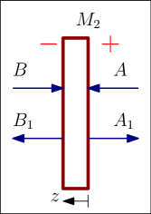
Figure 2: Scheme for simplest case of dispersive coupling. Movable mirror with amplitude reflectivity $R_{0}$ and transmittance $T_{0}$ is a free test mass, its position is measured by phase (phase quadrature) of reflected wave.

IV Simplest dispersive coupling

Here we consider simplest case of dispersive coupling. Movable mirror $M_{2}$ with amplitude reflectivity $R_{2}$ and transmittance $T_{2}$ is a free test mass, its position $z$ is measured by phase (phase quadrature) of reflected wave, see Fig.2. Again we consider case (9) (i.e. $B=0$ and $A$ is real). This scheme is widely known (for example, see Matsko et al. (1996)) and one can write down output small amplitudes

$$\hat{a}_{1} =T_{2}\hat{b}+R_{2}\hat{a}+AR_{2}\,2ikz,$$ (20a)

$$\hat{b}_{1} =T_{2}\hat{a}-R_{2}\hat{b}\,.$$ (20b)

We rewrite (20) for quadrature in frequency domain

$$a_{1a} =T_{2}b_{a}+R_{2}a_{a},$$ (21a)

$$a_{1p} =T_{2}b_{p}+R_{2}a_{p}+\sqrt{2}AR_{2}\,2kz(\Omega),$$ (21b)

$$b_{1a} =T_{2}a_{a}-R_{2}b_{a},$$ (21c)

$$b_{1p} =T_{2}a_{p}-R_{2}b_{p}$$ (21d)

We see that only phase quadrature $a_{1p}$ of reflected wave contains information on displacement.

Signal $F_{s}$ and fluctuation back action force (38) act on free test mass $m_{2}$ (it is a mass of movable mirror $M_{2}$). In case we (9) have obtain in frequency domain:

$$-m_{2}\Omega^{2}z=2\sqrt{2}\hslash kR_{2}A\left(R_{2}a_{a}+T_{2}b_{a}\frac{}{}\right)+F_{s}$$ (22)

Substituting (22) into (21) we obtain

$$a_{1a} =T_{2}b_{a}+R_{2}a_{a},$$ (23a)

$$a_{1p} =T_{2}b_{p}+R_{2}a_{p}-\mathcal{N}\,a_{1a}-\sqrt{2\mathcal{N}}\,f_{s},$$ (23b)

$$\mathcal{N}=\frac{8\hslash k^{2}R_{2}^{2}A^{2}}{m_{2}\Omega^{2}}$$ (23c)

Obviously, output quadratures $b_{1a},\ b_{1p}$ of transmitted wave do not contain any information on displacement $z$.

We see that equations (15) for dissipative coupling are similar to ones (23) for dispersive coupling. The difference is that phase quadrature $a_{a1}$ containing information on displacement in dispersive coupling (23) is replaced by amplitude quadrature $b_{1a}$ for dissipative coupling (15).

The formula (18) is valid also for dispersive coupling but with different homodyne angle: $\tan\theta=1/\mathcal{N}(\Omega_{0})$.

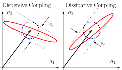
Figure 3: Squeezing of reflected wave on phase plane are denoted by ellipses for dissipative and dispersive couplings. Incident wave is in coherent state, its fluctuations are described by dotted circles.

Obviously both transforms (15) and (23) describe squeezing. The difference is illustrated on Fig. 3 if incident waves are in coherent state, which fluctuations are described by dotted circles. The reflected wave is squeezed (fluctuations denoted by ellipse): for dispersive coupling amplitude quadrature conserves and phase quadrature unsqueezes, whereas for dissipative coupling phase quadrature conserves and amplitude quadrature unsqueezes.

V Combined coupling

Let consider combined coupling when both dissipative and dispersive coupling take place. For it we analyse the same MSI on Fig. 1 but with movable BS, it is test mass $m_{bs}$ and coordinate is $y$ (1) and fixed mirror $M$ ($x=0$). Then using (33), (2) and (3) we obtain for small amplitudes:

$$a_{1} =-T_{0}b+R_{0}a+$$ (24a)

$$\quad+R_{0}B\sqrt{2}ky+T_{0}A\sqrt{2}ky-R_{0}A\,ik\sqrt{2}y,$$ (24b)

$$b_{1} =-T_{0}a-R_{0}b+$$ (24c)

$$\quad+R_{0}A\,k\sqrt{2}y-T_{0}B\,k\sqrt{2}y-R_{0}Bik\sqrt{2}y\,.$$ (24d)

In case of one pump (9) we rewrite input-output relations for quadratures in frequency domain:

$$a_{1a} =-T_{0}b_{a}+R_{0}a_{a}+T_{0}A2ky,$$ (25a)

$$a_{1p} =-T_{0}b_{p}+R_{0}a_{p}-R_{0}A\,2ky,$$ (25b)

$$b_{1a} =-T_{0}a_{a}-R_{0}b_{a}+R_{0}A\,2ky\,,$$ (25c)

$$b_{1p} =-T_{0}a_{p}-R_{0}b_{p}\,.$$ (25d)

We see that here both dissipative and dispersive coupling take place. Indeed, coordinate term in (25b) corresponds to dispersive coupling (compare with (21b)), whereas coordinate terms in (25a, 25c) — to dissipative coupling, compare with (12a, 12c).

Equations (25) should be supplemented by equation for mechanical degree of freedom. For coordinate $y$ we obtain using (36) in approximation (1) and (9) in frequency domain:

$$y =\frac{2\hslash kA\left(-R_{0}^{2}a_{a}+R_{0}T_{0}b_{a}+b_{p}\right)}{(K-m_{bs}\Omega^{2})}+$$ (26)

$$\quad+\frac{\sqrt{2\hbar m_{bs}\Omega^{2}}}{(K-m_{bs}\Omega^{2})}\cdot f_{s},$$ (27)

$$K=4\hslash k^{2}A^{2}R_{0}T_{0},\quad f_{s}=\frac{F_{s}}{\sqrt{2\hslash m_{bs}\Omega^{2}}},$$ (28)

where $f_{s}$ is signal force normalized to SQL, $K$ is optical rigidity, which appears due to existence of both dissipative and dispersive coupling. In order to have positive rigidity we should to keep $T_{0}R_{0}>0$, see definition (2). Note, rigidity $K$ is a constant, it does not depends on frequency.

The terms $\sim a_{a},\ b_{a}$ in (26) correspond to back action force of dispersive coupling, whereas term $\sim b_{p}$ in (26) — to back action force of dissipative coupling.

In order to apply idea of variation measurement we have to generalize it for two output beams. One can measure in transmitted and reflected waves arbitrary quadratures by homodyne detector and then take weighted sum of results. It means that we can take arbitrary linear combination of quadratures (25). Coefficients of this combination can be optimized to find minimum of PSD recalculated to $f_{s}$ (15) at some predefined frequency $\Omega_{0}$

$$S_{fs}^{\text{comb}}(\Omega) =\frac{1}{2LR_{0}}\times$$ (29a)

$$\times\left\{\frac{R_{0}^{2}+1}{T_{0}}\left[\frac{L_{0}-L}{L_{0}-1}\right]^{2}+\frac{T_{0}(L-1)^{2}}{\big{(}R_{0}^{2}+1\big{)}}\right\},$$

$$L =\frac{K}{m_{bs}\Omega^{2}},\quad L_{0}=\frac{K}{m_{bs}\Omega_{0}^{2}}$$ (29b)

See details in Appendix C. Recall that $S_{fs}^{\text{comb}}=1$ corresponds to SQL. At $\Omega=\Omega_{0}$ first term in (29) is equal to zero and second term defines minimum $S_{fs}^{\text{comb}}(\Omega_{0})$. However, at $\Omega=\Omega_{0}+\Delta\Omega$ the first term increases rather rapidly and defines effective bandwidth $\Gamma$. Requiring the increase of PSD by 2 times at $\Delta\Omega=\Gamma/2$ we find:

$$\frac{\Gamma}{\Omega_{0}} \simeq\frac{T_{0}(L_{0}-1)^{2}}{(R_{0}^{2}+1)L_{0}}\,,\quad\frac{\Gamma}{\Omega_{0}}\simeq 2R_{0}S_{fs}^{min}(\Omega_{0})$$ (30)

Here relation between bandwidth $\Gamma$ and $S_{fs}^{min}$ is similar to (19) and corresponds to known Cramer-Rao bound Mizuno (1996); Mizuno et al. (1993); Miao et al. (2017).

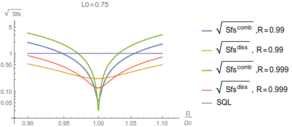
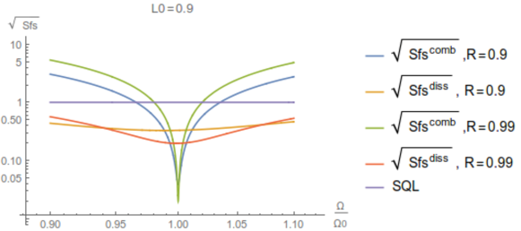
Figure 4: Plots of amplitude spectral densities $S_{fs}^{\text{comb}}(\Omega)$ and $S_{fs}^{\text{diss}}(\Omega)$ with the same pump power ($\hslash kA^{2}$ – const) for parameter $L_{0}=0.75$ (top) and $L_{0}=0.9$ (bottom) for different reflectivity $R_{0}$.

We see that structures of formulas for PSD $S_{fs}^{\text{comb}}$ and $S_{fs}^{\text{diss}}$ are similar. However, there is difference: at the same pump power one can get larger sensitivity (less $S_{fs}^{\text{comb}}$) for combined coupling than for dissipative one. Indeed, comparing (15b, 18) with (28, 29), we see that minimal PSD $S_{fs}^{\text{diss}}(\Omega_{0})$ for dissipative coupling and $S_{fs}^{\text{comb}}(\Omega_{0})$ are achieved at the same power if

$$\frac{2(L_{0}-1)^{2}}{R_{0}^{2}(1+R_{0}^{2})}=1.$$ (31)

For $R_{0}\simeq 1$ it means $L_{0}\simeq 2$. For close to resonance case (chosen frequency $\Omega_{0}$ is close to resonance one, or $(L_{0}-1)^{2}<1$) combined coupling gives larger sensitivity (smaller $S_{fs}^{\text{comb}}$) as compared with dissipative (as well as dispersive) coupling. Obviously, the physical reason is optical rigidity (28) which takes place for combined coupling only. The plots on Fig. 4 illustrate it.

VI Conclusion

We analysed the simplest (without cavity) variants of dissipative and dispersive opto-mechanical couplings and have shown that in case of dissipative coupling information on mechanical displacement as well as back action is in amplitude quadratures of reflected and transmitted waves. In contrast, for dispersive coupling information on displacement is in phase quadrature of reflected wave only, see Fig. 3.

We considered combined coupling based on Michelson-Sagnac interferometer (Fig. 1), when both dissipative and dispersive couplings takes place. For simplicity we considered the case without cavity and with one pump only. The main feature of combined coupling is optical rigidity (28), which appears as consequence of both kinds of couplings.

In spite of back action for pure dissipative and pure dispersive couplings acts in a different way, illustrated on Fig. 3, we have shown that variation measurement S.P. Vyatchanin and A.B. Matsko (1993); Vyatchanin and Zubova (1995); H.J. Kimble et al. (2001) can be applied for case of combined coupling. Moreover, at the same pump power one can surpass SQL more strongly than for pure dissipative (or dispersive) couplings. The physical reason of it is optical rigidity introduced by combined coupling.

Note, for combined coupling one has to use more complicated procedure of measurement with homodyne detection of both reflected and transmitted waves and taking optimal sum of them.

We would like to underline that we analysed simplest case of combined coupling without cavity. The case of combined coupling with cavity should be investigated separately, because of in this case we can use only one reflected wave (end mirror is assumed to be perfectly reflecting). For example, pure dissipative coupling, analysed in this paper, provides quantum transducer of displacement, whereas pure dissipative coupling in cavity gives quantum speed meter S.P. Vyatchanin and A.B. Matsko (2016), not a displacement meter.

Appendix A Analysis of MSI

Here we analyse MSI shown on dashed rectangle on Fig. 1 with 50/50 movable BS (coordinate $y$), movable completely reflected mirror $M$ (coordinate $x$). We calculate input-output relations and Lebedev forces acting on mirror $M$ and BS.

Complex wave amplitudes $\mathcal{A},\ \mathcal{A}_{1},\ \mathcal{B},\ \mathcal{B}_{1},\mathcal{A}_{n,e},\mathcal{B}_{n,e}$ are taken on non-shifted BS.

Input-output relations.

We start from equations:

$$\mathcal{A}_{e} =\frac{i\mathcal{B}+\mathcal{A}e^{-i\sqrt{2}ky_{bs}}}{\sqrt{2}},\quad\mathcal{A}_{n}=\frac{\mathcal{B}e^{i\sqrt{2}ky_{bs}}+i\mathcal{A}}{\sqrt{2}},$$ (32a)

$$\mathcal{A}_{1} =\frac{\mathcal{B}_{e}e^{-i\sqrt{2}ky_{bs}}+i\mathcal{B}_{n}}{\sqrt{2}},\quad\mathcal{B}_{1}=\frac{i\mathcal{B}_{e}+\mathcal{B}_{n}e^{i\sqrt{2}ky_{bs}}}{\sqrt{2}}$$

Where coordinates $$x_{m},\ y_{bs}$$ denote position of mirror M and BS. For waves incident on BS from inside MSI we have

$$\mathcal{B}_{e} =\mathcal{A}_{e}e^{-2ikx_{m}}e^{2i\phi_{e}},\quad\mathcal{B}_{n}=\mathcal{A}_{n}e^{2ikx_{m}}e^{2i\phi_{n}},$$ (32b)

where constants $\phi_{e,n}$ describe phase advance of wave travelling from BS to mirror $M$, when position of BS is $y_{bs}=0$ and position of mirror M is $x_{m}=0$. Substituting (32b) into (32a) and putting $e^{2i\phi_{e}}=1,\quad e^{2i\phi_{n}}=-1$, we obtain

$$\mathcal{A}_{1} =-\mathcal{B}T+e^{-ik\sqrt{2}y_{bs}}\mathcal{A}R,$$ (33a)

$$\mathcal{B}_{1} =-\mathcal{A}T-e^{ik\sqrt{2}y_{bs}}\mathcal{B}R,$$ (33b)

$$R =\cos k\big{(}2x_{m}+\sqrt{2}y_{bs}\big{)},\ T=-\sin k\big{(}2x_{m}+\sqrt{2}y_{bs}\big{)}.$$

So we can consider MSI as a GM with amplitude reflectivity $R$ and transmittance $T$.

Lebedev light pressure force $F_{m}$ acting on mirror $M$.

In general case

$$F_{m} =2\hslash k\left(|\mathcal{A}_{n}|^{2}-|\mathcal{A}_{e}|^{2}\right)=$$ (34a)

$$=2\hslash k\,i\left(\mathcal{A}\mathcal{B}^{*}e^{-ik\sqrt{2}y_{bs}}-\mathcal{A}^{*}\mathcal{B}e^{ik\sqrt{2}y_{bs}}\right)$$ (34b)

Here we used relations (32).

Lebedev light pressure force acting on BS

along axes $\xi,\ \eta$ on Fig. 1 are equal to

$$F_{\xi BS} =\hslash k\left(|\mathcal{B}|^{2}+|\mathcal{B}_{1}|^{2}-2|\mathcal{A}_{e}|^{2}\right),$$ (35a)

$$F_{\eta BS} =\hslash k\left(|\mathcal{A}|^{2}+|\mathcal{A}_{1}|^{2}-2|\mathcal{A}_{n}|^{2}\right).$$ (35b)

We see that light pressure force directed along axis $y$ is equal to

$$F_{bs} =\frac{F_{\xi BS}-F_{\eta BS}}{\sqrt{2}}=$$ (36a)

$$=\sqrt{2}\hslash k\left\{R^{2}\big{[}|\mathcal{B}|^{2}-|\mathcal{A}|^{2}\big{]}-\right.$$ (36b)

$$\quad\left.-RT\left(\mathcal{A}\mathcal{B}^{*}e^{-i\sqrt{2}ky_{bs}}+\mathcal{A}^{*}\mathcal{B}e^{i\sqrt{2}ky_{bs}}\right)\right\}+$$ (36c)

$$\quad+\sqrt{2}\hslash k\,i\left\{\mathcal{A}\mathcal{B}^{*}e^{-i\sqrt{2}ky_{bs}}-\mathcal{A}^{*}\mathcal{B}e^{i\sqrt{2}ky_{bs}}\right\}$$ (36d)

Here we used relations (32, 33) and put $y_{0}=0$ (defined in (1)). In light pressure force (36) terms (36b) and (36c) corresponds to dispersive coupling, whereas term (36d) — to dissipative one.

Appendix B Movable mirror

Here we analyse mirror $M1$ with reflectivity $R_{1}$ and transmittance $T_{1}$ which can move as a free test mass along axis $z$ as shown on Fig. 2. We calculate input-output relations and Lebedev forces acting on mirror.

Complex wave amplitudes $\mathcal{A},\ \mathcal{A}_{1},\ \mathcal{B},\ \mathcal{B}_{1}$ are taken on non-shifted mirror.

Input-output relations

are obvious

$$\mathcal{A}_{1} =\mathcal{B}T_{1}+e^{2ikz}\mathcal{A}R_{1},$$ (37a)

$$\mathcal{B}_{1} =\mathcal{A}T_{1}-e^{-2ikz}\mathcal{B}R_{1},$$ (37b)

Lebedev light pressure force $F_{m1}$ acting on mirror $M_{1}$:

$$F_{m1} =\hslash k\left(|\mathcal{A}|^{2}+|\mathcal{A}_{1}|^{2}-|\mathcal{B}|^{2}-|\mathcal{B}_{1}|^{2}\right)=$$ (38a)

$$=2\hslash k\,\left(R_{1}^{2}|\mathcal{A}|^{2}-R_{1}^{2}|\mathcal{B}|^{2}+\frac{}{}\right.$$ (38b)

$$\qquad\left.\frac{}{}+T_{1}R_{1}\left[\mathcal{A}\mathcal{B}^{*}e^{2ikz}+\mathcal{A}^{*}\mathcal{B}e^{-2ikz}\right]\right)$$ (38c)

Here we substitute (37) into (38a).

Appendix C Derivation of (29)

Let introduce notations for input and output amplitudes quadratures

$$d_{a} =R_{0}a_{a}-T_{0}b_{a},$$ (39a)

$$e_{a} =-T_{0}a_{a}-R_{0}b_{a}\,,$$ (39b)

$$g_{1a} =-T_{0}a_{1a}+R_{0}b_{1a},$$ (39c)

$$j_{1a} =R_{0}a_{1a}-T_{0}b_{1a}$$ (39d)

and rewrite (25) in form

$$g_{1a} =T_{0}d_{a}+R_{0}e_{a}++A2ky,$$ (40a)

$$j_{1a} =R_{0}d_{a}-T_{0}e_{a},$$ (40b)

$$a_{1p} =-T_{0}b_{p}+R_{0}a_{p}-R_{0}A\,2ky,$$ (40c)

$$b_{1p} =-T_{0}a_{p}-R_{0}b_{p},$$ (40d)

$$A2ky =\frac{L\left\{-R_{0}d_{a}+b_{p}\right\}}{(T_{0}R_{0})(L-1)}+\sqrt{\frac{2L}{T_{0}R_{0}}}\cdot\frac{f_{s}}{L-1},$$ (40e)

$$L =\frac{T_{0}R_{0}\,4\hslash k^{2}A^{2}}{m_{bs}\Omega^{2}},\quad f_{s}=\frac{F_{s}}{\sqrt{2\hslash m_{bs}\Omega^{2}}}$$ (40f)

Obviously, new quadratures $d_{a},\,e_{a},\,a_{p},\,b_{p}$ are not correlated with each other, creating orthogonal basis with PSD equal to:

$$S_{da} =1,\quad S_{ea}=1,\quad S_{ap}=1,\quad S_{bp}=1$$ (41)

Let we measure weighted sum

$$G =C\left(g_{1a}+A_{a}j_{1a}\right)+D\left(a_{1p}+A_{p}\tilde{b}_{1p}\right)=$$ (42a)

$$= \left\{C\big{[}T_{0}+A_{a}R_{0}\big{]}+\frac{R_{0}\big{(}DR_{0}-C\big{]}L}{T_{0}R_{0}(L-1)}\right\}d_{1a}-$$ (42b)

$$\quad-\left\{D\big{[}T_{0}+A_{p}R_{0}\big{]}+\frac{\big{(}DR_{0}-C\big{]}L}{T_{0}R_{0}(L-1)}\right\}\tilde{b}_{p}+$$ (42c)

$$\quad+C\big{[}R_{0}-A_{a}T_{0}\big{]}e_{1a}+D\big{[}R_{0}-A_{p}T_{0}\big{]}a_{p}+$$ (42d)

$$\qquad+\big{[}C-DR_{0}\big{]}\sqrt{\frac{2L}{T_{0}R_{0}}}\cdot\frac{f_{s}}{L-1}$$ (42e)

where $$A_{a},\ A_{p},\,C,\,D$$ are some constants to be found.

Lets require back action removal on given frequency $\Omega_{0}$. It means to equate to zero terms (42b, 42c) in (42) in order to find $A_{a},\ A_{p}$:

$$A_{a} =\frac{-1}{R_{0}}\left(T_{0}+\frac{\big{(}DR_{0}-C\big{]}L_{0}}{CT_{0}(L_{0}-1)}\right),\quad L_{0}=L(\Omega_{0})$$

$$A_{p} =\frac{-1}{DR_{0}}\left(DT_{0}+\frac{\big{(}DR_{0}-C\big{]}L_{0}}{T_{0}R_{0}(L_{0}-1)}\right).$$ (43a)

Now we substitute $A_{a},\ A_{p}$ into (42)

$$G =\frac{\big{[}C-DR_{0}\big{]}}{(L_{0}-1)}\sqrt{\frac{2L_{0}}{T_{0}R_{0}}}\times$$ (44a)

$$\left\{\sqrt{\frac{T_{0}R_{0}}{2L_{0}}}\left[\frac{DR_{0}L_{0}-C}{R_{0}(C-DR_{0})}\right]e_{1a}+\right.$$ (44b)

$$\left.+\sqrt{\frac{T_{0}R_{0}}{2L_{0}}}\left[\frac{2DR_{0}L_{0}-DR_{0}-CL_{0}}{R_{0}^{2}(C-DR_{0})}\right]a_{p}+f_{s}\right\}$$ (44c)

and calculate PSD, normalized to SQL

$$S_{fs}(\Omega_{0}) =\frac{T_{0}}{2R_{0}(C-DR_{0})^{2}}\times$$ (45a)

$$\left\{\left[DR_{0}\sqrt{L}_{0}-\frac{C}{\sqrt{L}_{0}}\right]^{2}+\right.$$ (45b)

$$\qquad\left.+\left[\frac{(2DR_{0}-C)\sqrt{L}_{0}}{R_{0}}-\frac{D}{\sqrt{L}_{0}}\right]^{2}\right\}$$ (45c)

Lets choose $D,\ C$ to minimize $S_{fs}(\Omega_{0})$. Obviously $S_{fs}(\Omega_{0})$ depends on ratio $D/C$ only:

$$\left.\frac{D}{C}\right|_{opt} =\frac{L_{0}+R_{0}^{2}}{R_{0}\left(L_{0}\big{[}R_{0}^{2}+2\big{]}-1\right)}.$$ (46)

So with optimal choice $D/C=(D/C)_{opt}$ PSD $S_{fs}^{min}$ at arbitrary frequency $\Omega$ is equal to (29).

References

• Aspelmeyer et al. (2014) M. Aspelmeyer, T. Kippenber, and F. Marquardt, Reviews of Modern Physics 86, 1391–1452 (2014).
• Povinelli et al. (2005) M. L. Povinelli, M. Lončar, M. Ibanescu, E. J. Smythe, S. G. Johnson, F. Capasso, and J. D. Joannopoulos, Opt. Lett. 30, 3042–3044 (2005), URL http://ol.osa.org/abstract.cfm?URI=ol-30-22-3042.
• Maslov et al. (2013) A. V. Maslov, V. N. Astratov, and M. I. Bakunov, Phys. Rev. A 87, 053848 (2013), URL http://link.aps.org/doi/10.1103/PhysRevA.87.053848.
• S.P. Vyatchanin and A.B. Matsko (1993) S.P. Vyatchanin and A.B. Matsko, Sov.Phys – JETP 77, 218–221 (1993).
• S.P. Vyatchanin and A.B. Matsko (1996) S.P. Vyatchanin and A.B. Matsko, Sov. Phys. – JETP 82, 107 (1996).
• A.B. Matsko and S.P. Vyatchanin (1997) A.B. Matsko and S.P. Vyatchanin, Applied Physics B 64, 167–171 (1997), ISSN 1432-0649, URL http://dx.doi.org/10.1007/s003400050161.
• H.J. Kimble et al. (2001) H.J. Kimble, Y. Levin, A.B. Matsko, K.S. Thorne, and S.P. Vyatchanin, Phys. Rev. D 65, 022002 (2001), eprint arXiv:gr-qc/0008026v2.
• V.B. Braginsky and F.Ya. Khalili. (1990) V.B. Braginsky and F.Ya. Khalili., Physics Letters A 147, 251–256 (1990).
• V.B. Braginsky et al. (2000) V.B. Braginsky, M.L. Gorodetsky, F.Y. Khalili, and K.S. Thorne, Physical Review D 61, 044002 (2000).
• LVC-Collaboration (2013) LVC-Collaboration, arXiv 1304.0670 (2013).
• J. Aasi et al et al.(2015) (LIGO Scientific Collaboration) J. Aasi et al (LIGO Scientific Collaboration) et al., Classical and Quantum Gravity 32, 074001 (2015).
• Martynov et al. (2016) D. Martynov et al., Physical Review D 93, 112004 (2016).
• Asernese et al. (2015) F. Asernese et al., Classical and Quantum Gravity 32, 024001 (2015).
• Dooley et al. (2016) K. L. Dooley, J. R. Leong, T. Adams, C. Affeldt, A. Bisht, C. Bogan, J. Degallaix, C. Graf, S. Hild, and J. Hough, Classical and Quantum Gravity 33, 075009 (2016).
• Aso et al. (2013) Y. Aso, Y. Michimura, K. Somiya, M. Ando, O. Miyakawa, T. Sekiguchi, and D. Tats, Physical Review D 88, 043007 (2013).
• M. Wu et al. (2014) M. Wu, A.C. Hryciw, C. Healey, D.P. Lake, H. Jayakumar, M.R. Freeman, J.P. Davis, and P.E. Barclay, Physical Review X 4, 021052 (2014).
• S. Forstner and S. Prams and J. Knittel and E.D. van Ooijen and J.D. Swaim and G.I. Harris and A. Szorkovszky and W.P. Bowen and H. Rubinsztein-Dunlop (2012) S. Forstner and S. Prams and J. Knittel and E.D. van Ooijen and J.D. Swaim and G.I. Harris and A. Szorkovszky and W.P. Bowen and H. Rubinsztein-Dunlop, Physical Review Letters 108, 120801 (2012).
• V.B. Braginsky (1968) V.B. Braginsky, Sov. Phys. JETP 26, 831–834 (1968).
• V.B. Braginsky and F.Ya. Khalili (1992) V.B. Braginsky and F.Ya. Khalili, Quantum Measurement (Cambridge University Press, Cambridge, 1992).
• Kippenberg and Vahala (2008) T. Kippenberg and K. Vahala, Science 321, 1172–1176 (2008).
• J.M. Dobrindt and T.J. Kippenberg (2010) J.M. Dobrindt and T.J. Kippenberg, Physical Review Letters 104, 033901 (2010).
• Vyatchanin and Zubova (1995) S. Vyatchanin and E. Zubova, Physics Letters A 201, 269–274 (1995).
• The LIGO Scientific collaboration (2011) The LIGO Scientific collaboration, Nature Physics 73, 962 (2011).
• LIGO Scientific Collaboration and Virgo Collaboration (2013) LIGO Scientific Collaboration and Virgo Collaboration, Nature Photonics 73, 613–619 (2013).
• Tse et al. (2019) V. Tse et al., Physical Review Letters 123, 231107 (2019).
• Asernese et al. (2019) F. Asernese, et al, and (Virgo Collaboration), Physical Review Letters 123, 231108 (2019).
• Yap et al. (2020) M. Yap, J. Cripe, G. Mansell, et al., Nature Photonics 14, 19–23 (2020).
• Yu et al. (2020) H. Yu et al., arXive 2002.01519 (2020).
• Cripe et al. (2019) J. Cripe, N. Aggarwal, R. Lanza, et al., Nature 568, 364–367 (2019).
• V.B. Braginsky and F.Ya. Khalili (1999) V.B. Braginsky and F.Ya. Khalili, Phys. Lett. A 257, 241 (1999).
• F.Ya. Khalili (2001) F.Ya. Khalili, Physics Letters A 288, 251–256 (2001), eprint arXiv:gr-qc/0107084.
• F. Elste and S.M. Girvin and A.A. Clerk (2009) F. Elste and S.M. Girvin and A.A. Clerk, Physical Review Letters 102, 207209 (2009).
• M. Li and W.H.P. Pernice and H.X. Tang (2009) M. Li and W.H.P. Pernice and H.X. Tang, Physical Review Letters 103, 223901 (2009).
• Weiss et al. (2013) T. Weiss, C. Bruder, and A. Nunnenkamp, New Journal of Physics 15, 045017 (2013).
• Hryciw et al. (2015) A. Hryciw, M. Wu, B. Khanaliloo, and P. Barclay, Optica 2, 491 (2015).
• Xuereb et al. (2011) A. Xuereb, R. Schnabel, and K. Hammerer, Physical Review Letters 107, 213604 (2011).
• Tarabrin et al. (2013) S. Tarabrin, H. Kaufer, F. Khalili, R. Schnabel, and K. Hammerer, Physical Review A 88, 023809 (2013).
• Sawadsky et al. (2015) A. Sawadsky, H. Kaufer, R. Nia, S. Tarabrin, F. Khalili, K. Hammerer, and R. Schnabel, Physical Review Letters 114, 043601 (2015).
• S. Huang and G.S. Agarwal (2010a) S. Huang and G.S. Agarwal, Physical Review A 81, 053810 (2010a).
• S. Huang and G.S. Agarwal (2010b) S. Huang and G.S. Agarwal, Physical Review A 82, 033811 (2010b).
• S.P. Vyatchanin and A.B. Matsko (2016) S.P. Vyatchanin and A.B. Matsko, Physical Review A 93, 063817 (2016).
• Mizuno (1996) J. Mizuno, Master’s thesis (1996), URL http://www2.mpq.mpg.de/~ros/geo600_docu/text/theses/Jun_Mizuno.pdf.
• Mizuno et al. (1993) J. Mizuno, K. Strain, P. Nelson, J. Chen, R. Schilling, A. Rüdiger, W. Winkler, and K. Danzmann, Physics Letters A 175, 273 (1993).
• Miao et al. (2017) H. Miao, R. Adhikari, Y. Ma, B. Pang, and Y. Chen, Physical Review Letters 119, 050801 (2017).
• Matsko et al. (1996) A. Matsko, E. Zubova, and S. Vyatchanin, Optics Communications 131, 107–113 (1996).