Accretion Disc-Jet Couplings in X-ray Binaries

Abstract

When the matter from a companion star is accreted towards the central compact accretor, i.e. a black hole (BH) or a neutron star (NS), an accretion disc and a jet outflow will form, providing bight X-ray and radio emission, which is known as X-ray binaries (XRBs). In the low/hard state, there exist disc-jet couplings in XRBs, but it remains uncertain whether the jet power comes from the disc or the central accretor. Moreover, BHXRBs have different properties compared with NSXRBs: quiescent BHXRBs are typically two to three orders of magnitude less luminous than NSXRBs in X-ray, whereas BHXRBs are more radio loud than NSXRBs. In observations, an empirical correlation has been established between radio and X-ray luminosity, $L_{\rm R}\propto L_{\rm X}^{b}$, where $b\sim 0.7$ for BHXRBs and $b\sim 1.4$ for non-pulsating NSXRBs. However, there are some outliers of BHXRBs showing unusually steep correlation as NSXRBs at higher luminosities. In this work, under the assumption that the origin of jet power is related to the internal energy of the inner disc, we apply our magnetized, radiatively efficient thin disc model and the well-known radiatively inefficient accretion flow model to NSXRBs and BHXRBs. We find that the observed radio/X-ray correlations in XRBs can be well understood by the disc-jet couplings.

1 Introduction

Most stars in the Universe are in the form of binary systems. When one of these two stars evolves into a black hole or a neutron star, its companion star may provide materials to be accreted by the compact object and form an accretion disc and a jet outflow. This process will release large amounts of gravitational energy and radiate bright X-ray from the disc, which is known as X-ray binaries (XRBs), together with radio emission from the jet. Generally, XRBs are classified into black hole X-ray binaries (BHXRBs) and neutron star X-ray binaries (NSXRBs) according to the type of central accretor. The radiation properties are quite different between BHXRBs and NSXRBs: in the quiescent state (QS), BHXRBs are typically two to three orders of magnitude less luminous than NSXRBs (Fender et al., 2003; Narayan & McClintock, 2008), but are more radio loud than NSXRBs, which indicates that the jet power in BHXRBs will be more powerful than that in NSXRBs; while in high/soft state (HSS), jet activities fade away for both BHXRBs and NSXRBs. In summery, we have the following relation for radio luminosities (related to jet activities) of different states:

$$L_{\rm R}^{\rm BH}({\rm QS})>L_{\rm R}^{\rm NS}({\rm QS})>L_{\rm R}({\rm HSS})\ .$$ (1)

In addition, how the relativistic jet forms, and how much power it carries are the key questions. It has long been suggested that relativistic jets could be powered not by the accretion flow but by the spin of the black hole (Blandford & Znajek, 1977; Narayan & McClintock, 2012). However, some scientists (Blandford & Payne, 1982; Fender et al., 2010) believe that the jet power mainly comes from the accretion disc rather than the spin of the black hole due to the disc-jet coupling phenomenon from observation. Corbel et al. (2003) discovered that, over four orders of magnitude in X-ray luminosity, the relation between radio and X-ray luminosity in the low/hard state (LHS) of the BHXRB GX 339-4 has the form of $L_{\mathrm{R}}\propto L_{\mathrm{X}}^{b}$, where $b\sim 0.7$ for $L_{\mathrm{X}}$ in the 3-9 keV range. Gallo et al. (2003) analysed a large sample of BHXRBs (including V404 Cyg, A0620-00) and extended this correlation down to the quiescent level, which is supposed to be a universal correlation between the radio and X-ray luminosity for BHXRBs. However, in recent years, some newly detected BHXRBs sources (e.g., H1743-322, Swift J1753.5-0127 and MAXI J1659-152) are found to lie significantly below the standard correlation (hereafter “outliers”). Coriat et al. (2011a) found BHXRB H1743-322 with a steeper correlation index of $b\sim 1.4$, but at lower luminosity it may return to the standard correlation, which presents an evidence for two different tracks for BHXRBs. Nowadays, the origin of these outliers are still under debate: on the one hand, Gallo et al. (2014); Gallo et al. (2018) argued that there is no statistical evidence for black hole systems following different tracks in the radio/X-ray luminosity plane; on the other hand, in the meantime, Islam & Zdziarski (2018) claimed that H1743-322 still follows different tracks from GX 339-4 when considering radio/bolometric flux correlations, which suggests that the accretion disc may undergo a morphological transition from radiatively inefficient to radiatively efficient flow (Koljonen & Russell, 2019).

As for NSXRBs, they are generally less radio loud for a given X-ray luminosity (regardless of mass differences for NS and BH) and they do not appear to show the strong suppression of radio emission in HSS that we observe in BHXRBs. However, recent studies (Tudor et al., 2017; Tetarenko et al., 2018) show that different NSXRB classes follow different correlations and normalizations in the radio/X-ray plane (possibly owing to the limited range of X-ray luminosities). Specifically, Migliari & Fender (2006) found that the correlation is consistent with $L_{\mathrm{R}}\propto L_{\mathrm{X}}^{1.4}$ including data taken from Aql X-1 and 4U 1728-34, over only one order of magnitude in X-ray luminosity. Tetarenko et al. (2016a) reported the third individual NSXRB simultaneous radio and X-ray measurements of EXO1745-248 and obtained its radio/X-ray correlation in the form of $L_{\mathrm{R}}\propto L_{\mathrm{X}}^{1.68}$. While pulsating systems such as accreting millisecond X-ray pulsars (AMXPs) and transitional millisecond X-ray pulsars (tMSPs) tend to show a shallower correlation $b\sim 0.7$ (Deller et al., 2015). Especially for the strongly magnetized accreting X-ray pulsar, they are likely to occupy a different radio/X-ray plane region with fainter radio luminosity (van den Eijnden et al., 2018; van den Eijnden et al., 2019). In this paper, we will focus on the non-pulsating NSXRBs with the steeper correlation $b\sim 1.4$, since the strong large-scale magnetic fields in X-ray pulsars can disrupt the inner disc and therefore the accretion disc may not extend to the NS surface.

It has been commonly believed that the correlation indexes of $\sim 1.4$ and $\sim 0.7$ correspond to a radiatively efficient and a radiatively inefficient accretion flows, respectively (Soleri et al., 2010; Coriat et al., 2011a; Jonker et al., 2012; Ratti et al., 2012; Russell et al., 2015; Plotkin et al., 2017). Table 1 present a concise comparisons among different accretion disc models. The luminous hot accretion flow (LHAF) proposed by Yuan (2001) and some magnetic accretion disc corona models (Merloni, 2003) can be applied to the radiatively efficient track. As for the radiatively inefficient track, it can be explained by the advection-dominated accretion flow (ADAF) (Narayan & Yi, 1994, 1995; Abramowicz et al., 1995) or some X-ray jet-dominated models (Markoff et al., 2003; Markoff et al., 2005). In previous researches (Narayan et al., 1997a, 1998; Narayan & McClintock, 2012), the ADAF model has been widely applied to BHXRBs, since the existence of horizon will not interrupt the process of advection, and the accreted matter can pass the horizon smoothly at a speed of light. However, things are quite different for NSXRBs: due to the substantial surface, there remains a caveat that the matter falling towards NS may be rebounded back, blocking up the advection-dominated flow. In this case, the ADAF model may not be well applicable to NSXRBs. Nevertheless, in order to explain the high frequency spectrum of NSXRBs, the disc ought to be optically thin. Except for ADAF, Shapiro et al. (1976) established an accretion disc model called Shapiro-Lightman-Eardley (SLE) disc, which is both optically and geometrically thin. Unfortunately, the original SLE disc was identified to be thermally unstable (Pringle, 1976; Piran, 1978), while later on Yu et al. (2015) found that the SLE disc could be stable when the small-scale turbulent magnetic pressure is strong enough, which is called the magnetized-SLE disc model (hereafter the M-thin disc). They showed that the M-thin disc is more likely to exist than other radiatively efficient disc models, and briefly indicated that it could be used to uncover the disc-jet couplings of XRBs.

In this paper, we take a further step to formulize the disc-jet coupling correlations based on the M-thin disc and the ADAF model, by assuming the jet power is related to the internal energy at the inner radius of the accretion disc. In Section 2, we introduce the equations of the M-thin disc and the ADAF model respectively, along with deducing the analytical radio/X-ray correlations with the aid of the aforementioned jet power assumption. The results for the theoretical temperature properties, as well as the comparison between theoretical regions with 35 observational XRB sources are presented in Section 3. Our conclusions and discussion are given in Section 4.

Table 1: Properties of different accretion disc models

Models	Optically	Geometrically	Thermally	Pressure	Cooling	Inner Disc $T_{\mathrm{i}}$	$L_{\mathrm{R}}\propto L_{\mathrm{X}}^{b}$
SSD	thick	thin	stable/unstable	gas/radiation	radiation	$\sim 10^{7}$ K	N/A
SLE	thin	thin	unstable	gas	radiation	$\sim 10^{9}$ K	N/A
ADAF	thin	thick	stable	gas	advection	$\sim 10^{11}$ K	$\sim 0.7$
LHAF	thin	thick	stable/unstable	gas	radiation	$\sim 10^{10}$ K	$\sim 1.4$
M-thin	thin	thin	stable	gas/magnetic	radiation	$\sim 10^{9}$ K	$\sim 1.4$

2 Equations

2.1 M-thin disc

The traditional SLE model follows these assumptions:

• The disc is assumed to rotate at $\Omega_{\mathrm{K}}$, which is the Keplerian angular velocity. We adopt that the general relativistic effect of the central accretor is simulated by the well-known pseudo-Newtonian potential introduced by Paczyńsky & Wiita (1980), i.e., $\Phi=-GM/(R-R_{\mathrm{s}})$, where $M$ is the mass of accretor, $R$ is the radius, and $R_{\mathrm{s}}=2GM/c^{2}$ is the Schwarzschild radius. Therefore, $\Omega=\Omega_{\mathrm{K}}=(GM/R)^{1/2}/(R-R_{\mathrm{s}})$;

• The vertical half thickness of the flow $H$ is smaller than the radius $R$, i.e. $H(R)=c_{\mathrm{s}}/\Omega_{\mathrm{K}}\lesssim R$, where $c_{\mathrm{s}}=\sqrt{p/\rho}$ is the isothermal local sound speed, with $p$ and $\rho$ being the pressure and mass density respectively;

• The kinematic viscosity coefficient $\nu$ is expressed as $\nu=\alpha c_{\mathrm{s}}H$, where $\alpha$ is the constant viscosity parameter.

Considering a vertically average, steady axis-symmetric accretion flow, we use unified steady state accretion flow equations introduced by Chen (1995):

$$\nu\Sigma=\frac{\dot{M}}{3\pi}fg^{-1}\ ,$$ (2)

where $\dot{M}$ is accretion rate, surface density $\Sigma=2H\rho$, $f=1-j/(\Omega R^{2})$, $g=-(2/3)(\mathrm{d}\ln\Omega_{\rm K}/\mathrm{d}\ln R)$ and $j$ is the specific angular momentum. When $\Omega=\Omega_{\mathrm{K}}$, $g=1+(2/3)/(R/R_{\rm s}-1)$, and

$$\dot{M}=-2\pi R\Sigma v_{\mathrm{R}}\ ,$$ (3)

where $v_{\mathrm{R}}$ is the radial velocity. To construct the energy conservation equation, we introduce the following assumptions:

• The dissipation energy goes into the ions;

• The energy is transferred from the ions to the electrons through Coulomb coupling;

• The electrons are cooled by bremsstrahlung process.

Based on these assumptions, the energy equations of the ions and electrons can be respectively written as

$$Q_{\mathrm{+}}=Q_{\mathrm{-}};\;Q_{\mathrm{-}}=\Lambda_{\mathrm{ie}};\;\Lambda_{\mathrm{ie}}=Q_{\mathrm{brems}}\ ,$$ (4)

where $Q_{\mathrm{+}}$ is the viscous heating rate per unit area, $Q_{\mathrm{-}}$ is the cooling rate per unit area, $\Lambda_{\mathrm{ie}}$ is the energy transfer rate from the ions to the electrons per unit area and $Q_{\mathrm{brems}}$ is the sum of radiatively cooling rate of electron per unit area. $Q_{\mathrm{+}}$ can be written as

$$Q_{\mathrm{+}}=\frac{3\dot{M}}{4\pi}\Omega^{2}fg\ .$$ (5)

$\Lambda_{\mathrm{ie}}$ is given by Kato et al. (2008):

$$\Lambda_{\mathrm{ie}}=\frac{3}{2}\nu_{\mathrm{E}}\frac{\Sigma k_{\rm B}(T_{\mathrm{i}}-T_{\mathrm{e}})}{m_{\mathrm{p}}}\ ,$$ (6)

where $k_{\rm B}$ is the Boltzmann constant, $m_{\mathrm{p}}$ is the proton mass, and $T_{\mathrm{i}}$ and $T_{\mathrm{e}}$ are the ion and electron temperatures, respectively. $\nu_{\mathrm{E}}=2.4\times 10^{21}\ln\Lambda~{}\rho\,T_{\mathrm{e}}^{-3/2}$, $\ln\Lambda$ is the Coulomb logarithm, here we take $\ln\Lambda=15$. Bremsstrahlung loss per unit volume from an electron gas is (Svensson, 1984):

$$q_{\mathrm{brems}}=\alpha_{\mathrm{f}}r_{\mathrm{e}}^{2}m_{\mathrm{e}}c^{3}n_{\mathrm{e}}^{2}f_{\mathrm{brems}}\ ,$$ (7)

where $\alpha_{\mathrm{f}}=e^{2}/2\pi\epsilon_{0}hc\approx 1/137$ is the fine-structure constant, $r_{\mathrm{e}}=e^{2}/m_{\mathrm{e}}c^{2}$ is the classical electron radius, and $n_{\mathrm{e}}$ is the electron number density. Here we assumed $n_{\mathrm{i}}=n_{\mathrm{e}}=\rho/m_{\mathrm{p}}$. $f_{\mathrm{brems}}$ is the dimensionless radiation rate due to relativistic bremsstrahlung, which can be decomposed into a part due to proton-electron collisions, $f_{\mathrm{ep}}$, and that due to electron-electron collisions, $f_{\mathrm{ee}}$, as

$$f_{\mathrm{brems}}=f_{\mathrm{ep}}+f_{\mathrm{ee}}\ ,$$ (8)

where $f_{\mathrm{ep}}$ and $f_{\mathrm{ee}}$ are approximated according to the following forms (Svensson, 1984):

$$f_{\mathrm{ep}}(\Theta_{\mathrm{e}})=\left\{\begin{array}[]{rl}12\Theta_{\mathrm{e}}\left(\mathrm{log}(2\,\eta_{\mathrm{E}}\,\Theta_{\mathrm{e}}+0.42)+\frac{3}{2}\right),&\Theta_{\mathrm{e}}>1\\[2.0pt] \frac{32}{3}\left(\frac{2}{\pi}\right)^{1/2}\Theta_{\mathrm{e}}^{1/2}(1+1.78\Theta_{\mathrm{e}}^{1.34}),&\Theta_{\mathrm{e}}<1\ ,\end{array}\right.$$ (9)

$$f_{\mathrm{ee}}(\Theta_{\mathrm{e}})=\left\{\begin{array}[]{rl}24\Theta_{\mathrm{e}}\left(\mathrm{log}(2\,\eta_{\mathrm{E}}\,\Theta_{\mathrm{e}})+\frac{5}{4}\right),&\Theta_{\mathrm{e}}>1\\[2.0pt] \frac{20}{9\pi^{1/2}}(44-3\pi^{2})^{1/2}\Theta_{\mathrm{e}}^{3/2}\times\\ (1+1.11\Theta_{\mathrm{e}}+\Theta_{\mathrm{e}}^{2}-1.25\Theta_{\mathrm{e}}^{2.5}),&\Theta_{\mathrm{e}}<1\ ,\end{array}\right.$$ (10)

where $\eta_{\mathrm{E}}=\mathrm{e}^{-\gamma_{\mathrm{E}}}$ and $\gamma_{\mathrm{E}}\approx 0.5772$ is the Euler constant, $\Theta_{\mathrm{e}}=k_{\rm B}\,T_{\mathrm{e}}/m_{\mathrm{e}}c^{2}$ the dimensionless electron temperature. The cooling rate per unit surface area of discs by bremsstrahlung is given by

$$Q_{\mathrm{brems}}=2Hq_{\mathrm{brems}}\ ,$$ (11)

where we neglect Compton amplification. Since the radiation pressure is negligible in optically thin discs, and we take the magnetic pressure into account in the M-thin disc, the total pressure $p$ is expressed as

$$p=p_{\mathrm{gas}}+p_{\mathrm{mag}}\ ,$$ (12)

where $p_{\mathrm{gas}}=\beta p$ is the gas pressure and $p_{\mathrm{mag}}=(1-\beta)p$ is the magnetic pressure. In this paper, we take $\beta=0.5$ in all calculations, which was previously adopted for global ADAF solutions (Narayan et al., 1997b), and was used in Yu et al. (2015) for the thermal stability analyses.

The gas is assumed to consist of protons and electrons, so the gas pressure $p_{\mathrm{gas}}$ is written as

$$p_{\mathrm{gas}}=\frac{\rho\,k_{\rm B}}{\mu\,m_{\mathrm{p}}}(T_{\mathrm{i}}+T_{\mathrm{e}})\ ,$$ (13)

where $\mu$ is the mean molecular weight, we set $\mu=1$ in this paper.

2.2 ADAF

Different from the M-thin disc, the ADAF is advection-dominated, thus we cannot expect angular velocity to be Keplerian. The original radial momentum equation in fluid dynamics is

$$v_{\mathrm{R}}\frac{\mathrm{d}v_{\mathrm{R}}}{\mathrm{d}R}-\Omega^{2}R=-\Omega^{2}_{\mathrm{K}}R-\frac{1}{\rho}\frac{\mathrm{d}}{\mathrm{d}R}(\rho c^{2}_{\mathrm{s}})\ .$$ (14)

We assume $v_{\mathrm{R}}\propto R^{-1/2}$, $\rho c_{\mathrm{s}}^{2}\propto R^{-5/2}$, the radial momentum equation is reduced to an algebraic form

$$-\frac{1}{2}\frac{v_{\mathrm{R}}^{2}}{R}-\Omega^{2}R=-\Omega_{\mathrm{K}}^{2}R+\frac{5}{2}\frac{c_{\mathrm{s}}^{2}}{R}\ .$$ (15)

$v_{\mathrm{R}}$ is negligible compared with $c_{\mathrm{s}}$, then we obtain the angular velocity in ADAFs:

$$\Omega^{2}=\Omega_{\mathrm{K}}^{2}-\frac{5}{2}\frac{c_{\mathrm{s}}^{2}}{R^{2}}\ .$$ (16)

Except for the angular velocity, another difference between the ADAF and the M-thin disc is the energy equation:

$$Q_{\mathrm{+}}=Q_{\mathrm{-}};\;Q_{\mathrm{-}}=\Lambda_{\mathrm{ie}}+Q_{\mathrm{adv}};\;\Lambda_{\mathrm{ie}}=Q_{\mathrm{brems}}\ .$$ (17)

The additional term $Q_{\mathrm{adv}}$ is the cooling rate per unit area by advection, which is given by (Chen & Taam, 1993):

$$Q_{\mathrm{adv}}=\frac{\dot{M}}{2\pi R^{2}}\frac{p}{\rho}\xi\ ,$$ (18)

where $\xi=-[(4-3\beta)/(\Gamma_{3}-1)](\mathrm{dln}T/\mathrm{dln}R)+(4-3\beta)(\mathrm{dln}\Sigma/\mathrm{dln}R)$, $\Gamma_{3}=1+(4-3\beta)(\gamma-1)/[\beta+12(\gamma-1)(\beta-1)]$, and $\gamma$ is the ratio of specific heats. For simplicity, we take $\xi=1$ into calculation.

Since the ADAF is a geometrically thick accretion disc, the outflow in the inner region ($R<100R_{\mathrm{s}}$) cannot be negligible. We assume the accretion rate varies as

$$\dot{M}=\dot{M}_{*}\frac{R}{100R_{\mathrm{s}}},\quad R<100R_{\mathrm{s}}\ ,$$ (19)

where $\dot{M}_{*}$ is the accretion rate at $R=100R_{\mathrm{s}}$. When $R>100R_{\mathrm{s}}$, $\dot{M}=\dot{M}_{*}$ at any given $R$.

Other assumptions and equations for the ADAF remain the same as the M-thin disc.

2.3 Analytical correlations

Except for numerical calculation, Fender et al. (2003) and Migliari & Fender (2006) obtain the indexes of radio/X-ray correlations via algebraic calculation. Analogously, we can also deduce these slope indexes from our model. For simplicity, in the following discussion, the accretion rate is given in the Eddington unit, i.e. $\dot{m}\equiv\dot{M}/\dot{M}_{\mathrm{Edd}}~{}(\dot{M}_{\mathrm{Edd}}\equiv L_{\mathrm{Edd}}/\eta c^{2})$, where $L_{\mathrm{Edd}}$ is the Eddington luminosity of $1.3\times 10^{38}(M/M_{\odot})\;\mathrm{erg/s}$, $\eta$ is the accretion efficiency of $\sim 1/16$ in the pseudo-Newtonian potential. The radius is also denoted in the Schwarzschild unit, i.e. $r=R/R_{\mathrm{s}}$.

Theoretically, the ADAF is usually applied to the inner region of the accretion disc for BHXRBs, the maximum ion temperature is around $10^{11}$K (Narayan & McClintock, 2008). Through our calculation, the maximum ion temperature of M-thin discs is significantly lower than ADAFs, which is around $10^{9}$K (see Figure 1 and Section 3 for details). Besides, an optically thick but geometrically thin standard Shakura-Sunyaev disc (SSD) was proposed to describe XRBs in HSS, whose maximum ion temperature is around $10^{7}$K (Shakura & Sunyaev, 1973). To sum up, the relation for temperatures of different accretion disc models are shown as:

$$T_{\mathrm{ADAF}}>T_{\mathrm{M-thin}}>T_{\mathrm{SSD}}\ ,$$ (20)

Comparing Equation (20) with Equation (1), we find that there remain some connections between jet power $L_{\mathrm{jet}}$ and internal energy rate $\dot{U}$ (since materials are accreting, energy per unit time is a meaningful term). The internal energy rate $\dot{U}$ can be estimated by

$$\dot{U}=\frac{3k\,T_{\mathrm{i}}^{\mathrm{max}}}{2\mu\,m_{\mathrm{p}}}\dot{M}\ .$$ (21)

If we assume the radio luminosity is related to internal energy rate, we can obtain the radio luminosity as

$$L_{\mathrm{R}}=f_{*}\dot{U}\ ,$$ (22)

where $f_{*}$ is the transferred fraction from internal energy rate to radio luminosity. Note that the value of $f_{*}$ should be relatively small since the fraction of the disc internal energy converting to the jet power is already a small value. Moreover, the portion of the jet emitting radio is also very small. Through fitting with the observational data, we set $f_{*}=10^{-6.5}$ for both M-thin discs and ADAFs. The X-ray luminosity can be obtained by integration:

$$L_{\mathrm{X}}=2\pi\int Q_{\mathrm{brems}}R\,\mathrm{d}R\ .$$ (23)

Since the X-ray luminosity is dominated by the inner region, we integrate it from the inner stable circular orbit $3R_{\mathrm{s}}$ to 100$R_{\mathrm{s}}$.

In ADAFs, the accretion flow is radiatively inefficient, the X-ray luminosity follows (Rees et al., 1982)

$$L_{\mathrm{X}}\propto\dot{m}^{2}\ .$$ (24)

The temperature of ADAFs is nearly independent of $\dot{m}$ (see Figure 2 and Section 3 for details),

$$L_{\mathrm{R}}=f_{*}\dot{U}=f_{*}\frac{3k\,T_{\mathrm{i}}^{\mathrm{max}}}{2\mu\,m_{\mathrm{p}}}\dot{M}\propto\dot{m}\ .$$ (25)

Thus the theoretical radio/X-ray correlation is given by $L_{\mathrm{R}}\propto L_{\mathrm{X}}^{0.5}$. As for the M-thin disc, the accretion flow is radiatively efficient, and the X-ray luminosity is proportional to the accretion rate

$$L_{\mathrm{X}}\propto\dot{m}\ .$$ (26)

Different from ADAFs, the temperature of M-thin discs is varied with accretion rate, we should deduce the correlation via basic energy equations (4). The viscous heating rate per unit area $Q_{\mathrm{+}}$ can be simplified as

$$Q_{\mathrm{+}}=\dot{m}F_{1}(r)\ ,$$ (27)

and the electron radiatively cooling rate per unit area $Q_{\mathrm{brems}}$ can be estimated by

$$Q_{\mathrm{brems}}=\Lambda_{\mathrm{ie}}=\dot{m}^{2}\frac{(T_{\mathrm{i}}-T_{\mathrm{e}})}{T_{\mathrm{e}}^{3/2}(T_{\mathrm{i}}+T_{\mathrm{e}})^{5/2}}F_{2}(r)\approx\frac{\dot{m}^{2}}{T_{\mathrm{i}}^{2}}F_{2}(r)\ ,$$ (28)

where $F_{1}(r),F_{2}(r)$ denote some complicated functions only varied with $r$. The thermal stability forces the M-thin disc to maintain $Q_{\mathrm{+}}=Q_{\mathrm{brems}}$ at any given $r$, which makes the temperature follow $T_{\mathrm{i}}\propto\dot{m}^{0.5}$ (this correlation is close to our numerical result $T_{\mathrm{i}}^{\mathrm{max}}\propto\dot{m}^{0.7}$ in Figure 2). Hence, the radio luminosity is given by

$$L_{\mathrm{R}}=f_{*}\dot{U}=f_{*}\frac{3k\,T_{\mathrm{i}}^{\mathrm{max}}}{2\mu\,m_{\mathrm{p}}}\dot{M}\propto\dot{m}^{0.5}\times\dot{m}=\dot{m}^{1.5}\ .$$ (29)

Therefore, the radio/X-ray correlation in the M-thin disc is approximately in the form of $L_{\mathrm{R}}\propto L_{\mathrm{X}}^{1.5}$.

3 Results

3.1 Temperature properties

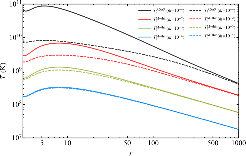
Figure 1: Radial variations of the ion temperature $T_{\mathrm{i}}$ (solid) and the electron temperature $T_{\mathrm{e}}$ (dashed) for $\dot{m}$ = 10^-4 (blue), 10^-3 (green), and 10^-2 (red) in M-thin discs ($M=1.4M_{\odot}$), as well as for ADAFs ($M=10M_{\odot}$, black), where $\alpha=0.1$, $j=1.8cR_{\mathrm{s}}$ in both models.

Based on the equations introduced above, we can calculate the temperature distributions for M-thin discs and ADAFs, respectively. We take $M=1.4M_{\odot}$ for M-thin discs and $M=10M_{\odot}$ for ADAFs. Figure 1 shows the radial variations of the ion and electron temperatures for M-thin discs and ADAFs with $\alpha=0.1$, $j=1.8cR_{\mathrm{s}}$. We can see that the ion temperature $T_{\mathrm{i}}$ (solid line) is significantly higher than the electron temperature $T_{\mathrm{e}}$ (dashed line) in the inner region of the disc. We set $\dot{m}$ = 10^-4 (blue), 10^-3 (green), and 10^-2 (red) for M-thin discs, and $\dot{m}_{*}$ = 10^-4 (black) for ADAFs (recall that $\dot{m}_{*}$ is the accretion rate given in Eddington unit at $R=100R_{\mathrm{s}}$). It is seen that the ion temperature of the ADAF is significantly higher than the M-thin disc, and they both have maximum ion temperature $T_{\mathrm{i}}^{\mathrm{max}}$ and maximum electron temperature $T_{\mathrm{e}}^{\mathrm{max}}$ in the inner region. When $\alpha=0.1$, $j=1.8cR_{\mathrm{s}}$, $T_{\mathrm{i}}^{\mathrm{max}}$ of the M-thin disc reaches $3.29\times 10^{8}$K, $1.31\times 10^{9}$K, $6.83\times 10^{9}$K for $\dot{m}=10^{-4},10^{-3},10^{-2}$, respectively, at $R=7.9R_{\mathrm{s}}$. As for ADAFs, $T_{\mathrm{i}}^{\mathrm{max}}$ remains $8.8\times 10^{10}$K at $R=5.4R_{\mathrm{s}}$, regardless of the variation of the accretion rate.

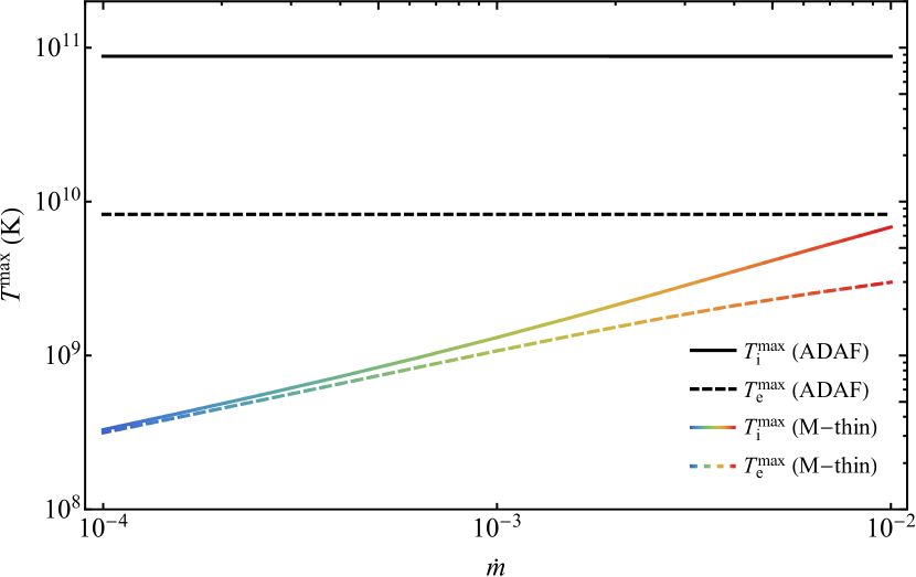
Figure 2: The maximum ion temperature $T_{\mathrm{i}}^{\mathrm{max}}$ (solid) and the maximum electron temperature $T_{\mathrm{e}}^{\mathrm{max}}$ (dashed) as a function of the accretion rate $\dot{m}$ for ADAFs ($M=10M_{\odot}$, black) and M-thin discs ($M=1.4M_{\odot}$, rainbow changing from blue to red as the temperature increases), where $\alpha=0.1$, $j=1.8cR_{\mathrm{s}}$ in both models.

Specifically in our calculation, $T_{\mathrm{i}}^{\mathrm{max}}$ and $T_{\mathrm{e}}^{\mathrm{max}}$ of ADAFs are nearly independent of $\dot{m}$, whereas the relation between $T_{\mathrm{i}}^{\mathrm{max}}$ and $\dot{m}$ in M-thin discs is close to $T_{\mathrm{i}}^{\mathrm{max}}\propto\dot{m}^{0.7}$, which is presented in Figure 2. Therefore, for clarity we only show the temperature distribution of ADAFs calculated by $\dot{m}_{*}=10^{-4}$ in Figure 1. Nevertheless, we point out that the value of $\alpha$ and $j$ can significantly change the temperature properties. For example, if we take $j=1.5cR_{\mathrm{s}}$ and $\alpha=0.3$, $T_{\mathrm{i}}^{\mathrm{max}}$ of M-thin discs will reach $1.74\times 10^{8}$K, $6.19\times 10^{8}$K, $2.87\times 10^{9}$K for $\dot{m}=10^{-4}$, 10^-3, 10^-2, respectively, at $R=3R_{\mathrm{s}}$, and $T_{\mathrm{i}}^{\mathrm{max}}$ of ADAFs will remain $3.77\times 10^{11}$K at $R=3R_{\mathrm{s}}$.

3.2 Theoretical regions

Now we can solve out the X-ray and radio luminosity theoretically when $M,\alpha,j,\dot{m}$ are given. Considering the observational data are scattered in some regions, it is reasonable for us to change above parameters within suitable ranges to create theoretical counterparts, comparing them with the observational data to verify our models.

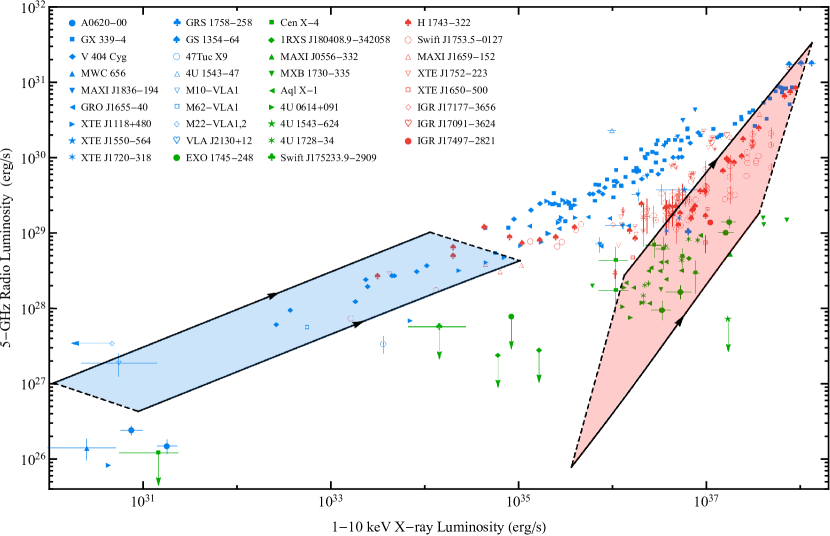
Figure 3: Radio (5 GHz) and X-ray (1-10 keV) luminosities for BHXRBs and NSXRBs (see Table 2 for references). Blue dots are data of BHXRBs following the standard radio/X-ray correlation; Red dots are data of BHXRB outliers; Green dots are data of non-pulsating NSXRBs. The blue region is calculated by ADAFs with $M=10M_{\odot}$, $\dot{m}_{*}=10^{-4}-10^{-2}$, where $\alpha=0.3$, $j=1.5cR_{\mathrm{s}}$ are given in the upper boundary and $\alpha=0.1$, $j=1.8cR_{\mathrm{s}}$ are given in the lower boundary, showing a slope of $\sim 0.5$; The red region is calculated by the M-thin disc with $\dot{m}=10^{-3}-10^{-1}$, where $M=10M_{\odot}$, $\alpha=0.01$, $j=1.8cR_{\mathrm{s}}$ are given in the upper boundary for BHXRBs outliers and $M=1.4M_{\odot}$, $\alpha=0.3$, $j=1.5cR_{\mathrm{s}}$ are given in the lower boundary for NSXRBs, showing a slope of $\sim 1.6$. Black arrows indicate the increase of the accretion rate; Colorful arrows denote the upper limits of the observational data.

Figure 3 illustrates two theoretical regions obtained by ADAFs and M-thin discs with different parametric ranges, whose black arrows in the upper/lower boundaries indicate the increase of the accretion rate. The blue region is calculated by ADAFs with $M=10M_{\odot}$ to explain the standard BHXRBs radio/X-ray correlation. In order to create a theoretical region, we firstly take $\alpha=0.3$ and $j=1.5cR_{\mathrm{s}}$ into the calculation, together with $\dot{m}_{*}$ changing from $10^{-4}$ to $10^{-2}$. The results are shown as the upper boundary of the blue region, where the radio and X-ray luminosities both increase as $\dot{m}_{*}$ goes up. Then we change $\alpha$ and $j$ into $0.1$ and $1.8cR_{\mathrm{s}}$, the corresponding results are given in the lower boundary of the region. Through adjusting $\alpha$ and $j$ linearly, we link the aforementioned two upper/lower boundaries with two dashed lines, which forms the theoretical ADAF region. Analogously, we can obtain the red region for BHXRBs outliers and NSXRBs by M-thin discs with $\dot{m}=10^{-3}-10^{-1}$, where $M=10M_{\odot}$, $\alpha=0.01$, $j=1.8cR_{\mathrm{s}}$ are given in the upper boundary for BHXRBs outliers, and $M=1.4M_{\odot}$, $\alpha=0.3$, $j=1.5cR_{\mathrm{s}}$ are set in the lower boundary for NSXRBs. Not only do the theoretical results of ADAFs and M-thin discs lie in different parts of the plane, but also they exhibit different slopes apparently. Our numerical solutions give 0.49 for ADAFs and 1.68 for M-thin discs, which are consistent with previous observational data fitting results within the range of errors.

3.3 Observations and correlations

Since the theoretical regions have already been obtained, we are able to introduce the simultaneous radio and X-ray observational data to verify our model assumptions. We adopt 35 XRB sources from the online repository (Bahramian et al., 2018), where all the measurements are converted to 5 GHz (in radio) and 1-10 keV (in X-rays), respectively, by assuming a flat radio spectral index and a power-law model in X-rays. For the standard radio/X-ray correlation of BHXRBs, we choose 17 sources: A0620-00, GX339-4, V404Cyg, MWC 656, MAXI J1836-194, GRO J1655-40, XTE J1118+480, XTE J1550-564, XTE J1720-318, GRS 1758-258, GS 1354-64, 47Tuc X9, 4U 1543-47, M10-VLA1, M62-VLA1, M22-VLA1,2 and VLA J2130+12, whose data are ranging from LHS to QS. As for NSXRBs, we only consider 10 non-pulsating sources: EXO 1745-248, Cen X-4, 1RXS J180408.9-342058, MAXI J0556-332, MXB 1730-335, Aql X-1, 4U 0614+091, 4U 1543-624, 4U 1728-34 and Swift J175233.9-2909. In terms of BHXRB outliers, we collect 8 sources, including H1743-322, Swift J1753.5-0127, MAXI J1659-152, IGR J17091-3624, IGR J17177-3656, IGR J17497-2821, XTE J1650-500 and XTE J1752-223. Their corresponding references are listed individually in Table 2.

Figure 3 denotes three types of sources in three colours: blue dots are data of BHXRBs following the standard radio/X-ray correlation; red dots are data of BHXRB outliers; green dots are data of non-pulsating NSXRBs. Different types of data lie well inside the corresponding theoretical regions and show nearly the same slope as the theoretical expectation. However, due to the fact that there is no solution for ADAFs for large radii if $\dot{m}>0.01$, our blue region cannot cover data of standard BHXRBs at high luminosity, which indicates that the ADAF is applicable to the QS and the LHS. As for BHXRBs at high X-ray luminosity, the LHAF model may be a promising model to understand their behaviour (Coriat et al., 2011a; Koljonen & Russell, 2019).

4 Conclusions and discussion

Table 2: References of 35 simultaneous radio and X-ray sources

Sources	Types	References
A0620-00	BHXRB	Gallo et al. 2006; Dinçer et al. 2017; Jonker & Nelemans 2004
GX 339-4	BHXRB	Corbel et al. 2013; Zdziarski et al. 2004
V 404 Cyg	BHXRB	Corbel et al. 2008; Miller-Jones et al. 2009; Rana et al. 2016; Plotkin et al. 2017
MWC 656	BHXRB	Ribó et al. 2017
MAXI J1836-194	BHXRB	Russell et al. 2015
GRO J1655-40	BHXRB	Coriat et al. 2010; Calvelo et al. 2010
XTE J1118+480	BHXRB	Fender et al. 2010; Gallo et al. 2014
XTE J1550-564	BHXRB	Gallo et al. 2003
XTE J1720-318	BHXRB	Brocksopp et al. 2005
GRS 1758-258	BHXRB	Gallo et al. 2003
GS 1354-64	BHXRB	Gallo et al. 2003
47Tuc X9	BHXRB	Miller-Jones et al. 2015; Bahramian et al. 2017
4U 1543-47	BHXRB	Gallo et al. 2003
M10-VLA1	BHXRB	Shishkovsky et al. 2018.
M62-VLA1	BHXRB	Chomiuk et al. 2013
M22-VLA1,2	BHXRB	Strader et al. 2012
VLA J2130+12	BHXRB	Tetarenko et al. 2016b
EXO 1745-248	NSXRB	Valenti et al. 2007; Tetarenko et al. 2016a
Cen X-4	NSXRB	Tudor et al. 2017
1RXS J180408.9-342058	NSXRB	Gusinskaia et al. 2017
MAXI J0556-332	NSXRB	Coriat et al. 2011b
MXB 1730-335	NSXRB	Rutledge et al. 1998
Aql X-1	NSXRB	Jonker & Nelemans 2004; Tudose et al. 2009; Miller-Jones et al. 2010; Migliari et al. 2011
4U 0614+091	NSXRB	Migliari et al. 2011
4U 1543-624	NSXRB	Ludlam et al. 2017
4U 1728-34	NSXRB	Migliari et al. 2003; Galloway et al. 2003; Migliari et al. 2011
Swift J175233.9-2909	NSXRB	Tetarenko et al. 2017
H 1743-322	BH Outlier	Coriat et al. 2011a
Swift J1753.5-0127	BH Outlier	Zurita et al. 2008; Soleri et al. 2010; Rushton et al. 2016; Plotkin et al. 2017
MAXI J1659-152	BH Outlier	Jonker et al. 2012
XTE J1752-223	BH Outlier	Ratti et al. 2012; Brocksopp et al. 2013
XTE J1650-500	BH Outlier	Corbel et al. 2004
IGR J17177-3656	BH Outlier	Paizis et al. 2011
IGR J17091-3624	BH Outlier	Rodriguez et al. 2011
IGR J17497-2821	BH Outlier	Rodriguez et al. 2007

In this work, we have applied the magnetized, optically and geometrically thin, two-temperature, radiative cooling-dominated accretion disc (the M-thin disc) to BHXRB outliers and non-pulsating NSXRBs. We have also calculated the ADAF for standard BHXRBs. Firstly, we have derived the ion and electron temperatures as a function of radius and accretion rate for both models. Then we investigated the relations between radio luminosity and temperatures, and assumed that the jet power is offered by a fraction of the internal energy from the accretion disc. We used the maximum ion temperature for an estimation of the internal energy rate and calculated the theoretical X-ray and radio luminosity. Moreover, we have also deduced the powerlaw indexes 0.5 and 1.5 for BHXRBs and NSXRBs via ADAFs and M-thin discs, respectively, and have found the two different theoretical regions well match the observational data. Therefore, the black hole system may have two choices, i.e., either the ADAF or the M-thin disc, whose slope corresponds to $\sim 0.5$ (radiatively inefficient) and $\sim 1.5$ (radiatively efficient), respectively.

Recently, Tremou et al. (2020) reported new simultaneous radio/X-ray measurements of the quiescent GX 339-4, which well lie inside the ADAF region in Figure 3. Nonetheless at the same time, Yan et al. (2020) found an unexpected “cooler when fainter” (positive $T_{\mathrm{e}}-L_{\mathrm{X}}$ correlation) branch in the low-luminosity regime ($L_{\mathrm{X}}<3\times 10^{36}$ erg s^-1), which puts a challenge to the classic ADAF model. On the other hand, as shown by our Figure 1, the M-thin disc may well explain such a correlation.

Nevertheless, we should point out that in order to simplify the analysis and the calculation, some simple assumptions have been made in our models. For instance, several parameters (e.g., the magnetic pressure $\beta$, the transferred fraction $f^{*}$) are assumed to be constant, together with a flat spectral index in the observational data. It is worth evaluating our models under more variables and a non-flat spectral index (Espinasse & Fender, 2018) in further studies; Except for the power of jets, there are other factors (e.g., the mass of the compact object in Körding et al. 2006, radiative efficiency in Yuan & Narayan 2014, inclination of the binary system in Motta et al. 2018) could mildly affect the radio luminosity, and it would be interesting to take these factors into consideration in future works; Only the bremsstrahlung cooling process is taken into account, which indicates temperatures in the real cases may be lower than the current solutions. In addition, we should note that the M-thin disc model is limited to the non-pulsating NSXRBs, while it is of great interest to develop new accretion disc models (e.g, the magnetic flux-dominated jet model proposed by Parfrey et al. 2016) to understand the disc-jet couplings in pulsating NSXRBs.

However, in our opinion, these assumptions are valid for us to make a comparison between theoretical results and observational data over orders of magnitude, delivering fruitful insights of the disc-jet couplings of BHXRBs and non-pulsating NSXRBs, along with revealing the potential connections between the jet power and the internal energy of the inner accretion disc.

References

- Abramowicz et al. (1995) Abramowicz M. A., Chen X., Kato S., Lasota J.-P., Regev O., 1995, ApJ, 438, L37
- Bahramian et al. (2017) Bahramian A., et al., 2017, MNRAS, 467, 2199
- Bahramian et al. (2018) Bahramian A., et al., 2018, Radio/X-Ray Correlation Database for X-Ray Binaries, doi:10.5281/zenodo.1252036
- Blandford & Payne (1982) Blandford R. D., Payne D. G., 1982, MNRAS, 199, 883
- Blandford & Znajek (1977) Blandford R. D., Znajek R. L., 1977, MNRAS, 179, 433
- Brocksopp et al. (2005) Brocksopp C., Corbel S., Fender R. P., Rupen M., Sault R., Tingay S. J., Hannikainen D., O’Brien K., 2005, MNRAS, 356, 125
- Brocksopp et al. (2013) Brocksopp C., Corbel S., Tzioumis A., Broderick J. W., Rodriguez J., Yang J., Fender R. P., Paragi Z., 2013, MNRAS, 432, 931
- Calvelo et al. (2010) Calvelo D. E., et al., 2010, MNRAS, 409, 839
- Chen (1995) Chen X., 1995, MNRAS, 275, 641
- Chen & Taam (1993) Chen X., Taam R. E., 1993, ApJ, 412, 254
- Chomiuk et al. (2013) Chomiuk L., Strader J., Maccarone T. J., Miller-Jones J. C. A., Heinke C., Noyola E., Seth A. C., Ransom S., 2013, ApJ, 777, 69
- Corbel et al. (2003) Corbel S., Nowak M. A., Fender R. P., Tzioumis A. K., Markoff S., 2003, A&A, 400, 1007
- Corbel et al. (2004) Corbel S., Fender R. P., Tomsick J. A., Tzioumis A. K., Tingay S., 2004, ApJ, 617, 1272
- Corbel et al. (2008) Corbel S., Koerding E., Kaaret P., 2008, MNRAS, 389, 1697
- Corbel et al. (2013) Corbel S., Coriat M., Brocksopp C., Tzioumis A. K., Fender R. P., Tomsick J. A., Buxton M. M., Bailyn C. D., 2013, MNRAS, 428, 2500
- Coriat et al. (2010) Coriat M., et al., 2010, IAU Symp., 6, 255
- Coriat et al. (2011a) Coriat M., et al., 2011a, MNRAS, 414, 677
- Coriat et al. (2011b) Coriat M., Tzioumis T., Corbel S., Fender R., Brocksopp C., Broderick J., Casella P., Maccarone T., 2011b, ATel, 3119
- Deller et al. (2015) Deller A. T., et al., 2015, ApJ, 809, 13
- Dinçer et al. (2017) Dinçer T., Bailyn C. D., Miller-Jones J. C. A., Buxton M., MacDonald R. K. D., 2017, ApJ, 852, 4
- Espinasse & Fender (2018) Espinasse M., Fender R., 2018, MNRAS, 473, 4122
- Fender et al. (2003) Fender R. P., Gallo E., Jonker P. G., 2003, MNRAS, 343, L99
- Fender et al. (2010) Fender R. P., Gallo E., Russell D., 2010, MNRAS, 406, 1425
- Gallo et al. (2003) Gallo E., Fender R. P., Pooley G. G., 2003, MNRAS, 344, 60
- Gallo et al. (2006) Gallo E., Fender R. P., Miller-Jones J. C. A., Merloni A., Jonker P. G., Heinz S., Maccarone T. J., Van Der Klis M., 2006, MNRAS, 370, 1351
- Gallo et al. (2014) Gallo E., et al., 2014, MNRAS, 445, 290
- Gallo et al. (2018) Gallo E., Degenaar N., van den Eijnden J., 2018, MNRAS, 478, L132
- Galloway et al. (2003) Galloway D. K., Psaltis D., Chakrabarty D., Muno M. P., 2003, ApJ, 590, 999
- Gusinskaia et al. (2017) Gusinskaia N. V., et al., 2017, MNRAS, 470, 1871
- Islam & Zdziarski (2018) Islam N., Zdziarski A. A., 2018, MNRAS, 481, 4513
- Jonker & Nelemans (2004) Jonker P. G., Nelemans G., 2004, MNRAS, 354, 355
- Jonker et al. (2012) Jonker P. G., Miller-Jones J. C. A., Homan J., Tomsick J., Fender R. P., Kaaret P., Markoff S., Gallo E., 2012, MNRAS, 423, 3308
- Kato et al. (2008) Kato S., Fukue J., Mineshige S., 2008, Black-Hole Accretion Disks: Towards a New Paradigm. Kyoto University Press, Kyoto, Japan
- Koljonen & Russell (2019) Koljonen K. I. I., Russell D. M., 2019, ApJ, 871, 26
- Körding et al. (2006) Körding E., Falcke H., Corbel S., 2006, A&A, 456, 439
- Ludlam et al. (2017) Ludlam R., Miller J. M., Miller-Jones J., Reynolds M., 2017, ATel, 0690
- Markoff et al. (2003) Markoff S., Nowak M., Corbel S., Fender R., Falcke H., 2003, A&A, 397, 645
- Markoff et al. (2005) Markoff S., Nowak M. A., Wilms J., 2005, ApJ, 635, 1203
- Merloni (2003) Merloni A., 2003, MNRAS, 341, 1051
- Migliari & Fender (2006) Migliari S., Fender R. P., 2006, MNRAS, 366, 79
- Migliari et al. (2003) Migliari S., Fender R. P., Rupen M., Jonker P. G., Klein-Wolt M., Hjellming R. M., van der Klis M., 2003, MNRAS, 342, L67
- Migliari et al. (2011) Migliari S., Miller-Jones J. C. A., Russell D. M., 2011, MNRAS, 415, 2407
- Miller-Jones et al. (2009) Miller-Jones J. C. A., Jonker P. G., Dhawan V., Brisken W., Rupen M. P., Nelemans G., Gallo E., 2009, ApJ, 706, L230
- Miller-Jones et al. (2010) Miller-Jones J. C. A., et al., 2010, ApJL, 716, L109
- Miller-Jones et al. (2015) Miller-Jones J. C. A., et al., 2015, MNRAS, 453, 3918
- Motta et al. (2018) Motta S. E., Casella P., Fender R. P., 2018, MNRAS, 478, 5159
- Narayan & McClintock (2008) Narayan R., McClintock J. E., 2008, New Astron. Rev., 51, 733
- Narayan & McClintock (2012) Narayan R., McClintock J. E., 2012, MNRAS, 419, L69
- Narayan & Yi (1994) Narayan R., Yi I., 1994, ApJ, 428, L13
- Narayan & Yi (1995) Narayan R., Yi I., 1995, ApJ, 444, 231
- Narayan et al. (1997a) Narayan R., Garcia M. R., McClintock J. E., 1997a, ApJ, 478, L79
- Narayan et al. (1997b) Narayan R., Kato S., Honma F., 1997b, ApJ, 476, 49
- Narayan et al. (1998) Narayan R., Mahadevan R., Quataert E., 1998, in Abramowicz M. A., Bjornsson G., Pringle J. E., eds, Theory of Black Hole Accretion Disks. Cambridge Univ. Press, Cambridge, p. 148
- Paczyńsky & Wiita (1980) Paczyńsky B., Wiita P. J., 1980, A&A, 88, 23
- Paizis et al. (2011) Paizis A., et al., 2011, ApJ, 738, 183
- Parfrey et al. (2016) Parfrey K., Spitkovsky A., Beloborodov A. M., 2016, ApJ, 822, 33
- Piran (1978) Piran T., 1978, ApJ, 221, 652
- Plotkin et al. (2017) Plotkin R. M., et al., 2017, ApJ, 834, 104
- Pringle (1976) Pringle J. E., 1976, MNRAS, 177, 65
- Rana et al. (2016) Rana V., et al., 2016, ApJ, 821, 103
- Ratti et al. (2012) Ratti E. M., et al., 2012, MNRAS, 423, 2656
- Rees et al. (1982) Rees M. J., Begelman M. C., Blandford R. D., Phinney E. S., 1982, Nature, 295, 17
- Ribó et al. (2017) Ribó M., et al., 2017, ApJL, 835, L33
- Rodriguez et al. (2007) Rodriguez J., Bel M. C., Tomsick J. A., Corbel S., Brocksopp C., Paizis A., Shaw S. E., Bodaghee A., 2007, ApJ, 655, L97
- Rodriguez et al. (2011) Rodriguez J., Corbel S., Caballero I., Tomsick J. A., Tzioumis T., Paizis A., Bel M. C., Kuulkers E., 2011, A&A, 533, L4
- Rushton et al. (2016) Rushton A. P., et al., 2016, MNRAS, 463, 628
- Russell et al. (2015) Russell T. D., et al., 2015, MNRAS, 450, 1745
- Rutledge et al. (1998) Rutledge R., Moore C., Fox D., Lewin W., van Paradijs J., 1998, ATel, 8
- Shakura & Sunyaev (1973) Shakura N. I., Sunyaev R. A., 1973, X- Gamma-Ray Astron., 55, 155
- Shapiro et al. (1976) Shapiro S. L., Lightman A. P., Eardley D. M., 1976, ApJ, 204, 187
- Shishkovsky et al. (2018) Shishkovsky L., et al., 2018, ApJ, 855, 55
- Soleri et al. (2010) Soleri P., et al., 2010, MNRAS, 406, 1471
- Strader et al. (2012) Strader J., Chomiuk L., Maccarone T. J., Miller-Jones J. C. A., Seth A. C., 2012, Nature, 490, 71
- Svensson (1984) Svensson R., 1984, MNRAS, 209, 175
- Tetarenko et al. (2016a) Tetarenko A. J., et al., 2016a, MNRAS, 460, 345
- Tetarenko et al. (2016b) Tetarenko B. E., et al., 2016b, ApJ, 825, 10
- Tetarenko et al. (2017) Tetarenko A. J., et al., 2017, ATel, 0422
- Tetarenko et al. (2018) Tetarenko A. J., et al., 2018, ApJ, 854, 125
- Tremou et al. (2020) Tremou E., et al., 2020, MNRAS, 493, L132
- Tudor et al. (2017) Tudor V., et al., 2017, MNRAS, 470, 324
- Tudose et al. (2009) Tudose V., Fender R. P., Linares M., Maitra D., Van Der Klis M., 2009, MNRAS, 400, 2111
- Valenti et al. (2007) Valenti E., Ferraro F. R., Origlia L., 2007, AJ, 133, 1287
- Yan et al. (2020) Yan Z., Xie F.-G., Zhang W., 2020, ApJL, 889, L18
- Yu et al. (2015) Yu X.-F., Gu W.-M., Liu T., Ma R.-Y., Lu J.-F., 2015, ApJ, 801, 47
- Yuan (2001) Yuan F., 2001, MNRAS, 324, 119
- Yuan & Narayan (2014) Yuan F., Narayan R., 2014, ARA&A, 52, 529
- Zdziarski et al. (2004) Zdziarski A. A., Gierlinski M., Mikolajewska J., Wardzinski G., Smith D. M., Alan Harmon B., Kitamoto S., 2004, MNRAS, 351, 791
- Zurita et al. (2008) Zurita C., Durant M., Torres M. a. P., Shahbaz T., Casares J., Steeghs D., 2008, ApJ, 681, 1458
- van den Eijnden et al. (2018) van den Eijnden J., Degenaar N., Russell T. D., Wijnands R., Miller-Jones J. C. A., Sivakoff G. R., Hernández Santisteban J. V., 2018, Nature, 562, 233
- van den Eijnden et al. (2019) van den Eijnden J., Degenaar N., Russell T. D., Hernández Santisteban J. V., Wijnands R., Miller-Jones J. C. A., Rouco Escorial A., Sivakoff G. R., 2019, MNRAS, 483, 4628