The Spectacular Ultraviolet Flash From the
Peculiar Type Ia Supernova 2019yvq

Abstract

Early observations of Type Ia supernovae (SNe Ia) provide essential clues for understanding the progenitor system that gave rise to the terminal thermonuclear explosion. We present exquisite observations of SN 2019yvq, the second observed SN Ia, after iPTF 14atg, to display an early flash of emission in the ultraviolet (UV) and optical. Our analysis finds that SN 2019yvq was unusual, even when ignoring the initial flash, in that it was moderately underluminous for an SN Ia ($M_{g}\approx-18.5$ mag at peak) yet featured very high absorption velocities ($v\approx 15,000$ km s^-1 for Si II $\lambda$6355 at peak). We find that many of the observational features of SN 2019yvq, aside from the flash, can be explained if the explosive yield of radioactive ⁵⁶Ni is relatively low (we measure $M_{{}^{56}\mathrm{Ni}}=0.31\pm 0.05\,M_{\odot}$) and it and other iron-group elements are concentrated in the innermost layers of the ejecta. To explain both the UV/optical flash and peak properties of SN 2019yvq we consider four different models: interaction between the SN ejecta and a nondegenerate companion, extended clumps of ⁵⁶Ni in the outer ejecta, a double-detonation explosion, and the violent merger of two white dwarfs. Each of these models has shortcomings when compared to the observations; it is clear additional tuning is required to better match SN 2019yvq. In closing, we predict that the nebular spectra of SN 2019yvq will feature either H or He emission, if the ejecta collided with a companion, strong [Ca II] emission, if it was a double detonation, or narrow [O I] emission, if it was due to a violent merger.

1 Introduction

There is now no doubt that Type Ia supernovae (SNe Ia) are the result of thermonuclear explosions in C/O white dwarfs (WDs) in multiple star systems (see, e.g., Maoz et al., 2014, and references therein). Despite this certainty, the nature of the binary companion, which plays an essential role in driving the primary WD toward explosion, remains highly uncertain.

Historically, most studies have focused on whether or not the companion is also a WD, the double degenerate (DD) scenario (e.g., Webbink, 1984), or some other nondegenerate star, the single degenerate (SD) scenario (e.g., Whelan & Iben, 1973). In addition to this fundamental question, recent efforts have also focused on whether or not sub-Chandrasekhar mass WDs can explode (e.g., Fink et al., 2010; Scalzo et al., 2014b; Shen & Bildsten, 2014; Polin et al., 2019a; Gronow et al., 2020) and the specific scenario in which the WD explodes (see Hillebrandt et al., 2013; Röpke & Sim, 2018, and references therein).

Unfortunately, maximum-light observations of SNe Ia have not provided the discriminatory power necessary to answer these questions and infer the progenitor system (e.g., Röpke et al., 2012). It has recently been recognized that extremely early observations, in the hours to days after explosion, may help to constrain which progenitor scenarios are viable and which are not. In particular, Kasen (2010) showed that for favorable configurations in the SD scenario, the SN ejecta will collide with the nondegenerate companion producing a shock that gives rise to an ultraviolet (UV)/optical flash in excess of the typical emission from an SN Ia.

The findings in Kasen (2010) launched a bevy of studies to search for such a signal (e.g., Hayden et al., 2010; Bianco et al., 2011; Ganeshalingam et al., 2011; Nugent et al., 2011; Olling et al., 2015), including several claims of a detection of the interaction with a nondegenerate companion (e.g., Cao et al. 2015; Marion et al. 2016; Hosseinzadeh et al. 2017; Dimitriadis et al. 2019; though see also Kromer et al. 2016; Jiang et al. 2018; Shappee et al. 2018, 2019 for alternative explanations). In the meantime, it has been found that an early optical bump, or flash, in the light curves of SNe Ia is not uniquely limited to the SD scenario (e.g., Raskin & Kasen, 2013; Piro & Morozova, 2016; Jiang et al., 2017; Levanon & Soker, 2017; Noebauer et al., 2017; Maeda et al., 2018; De et al., 2019; Polin et al., 2019a; Magee & Maguire, 2020).

Despite some observational degeneracies, early observations have and will continue to play a critical role in understanding the progenitors of SNe Ia (e.g., early photometry of SN 2011fe constrained the size of the exploding star to be $\lesssim 0.02$ $R_{\odot}$, providing the most direct evidence to date that SNe Ia come from WDs; Bloom et al., 2012).

Here we present X-ray, UV, and optical observations of the spectacular SN 2019yvq, only the second observed SN Ia, after iPTF 14atg (Cao et al., 2015), to exhibit an early UV flash. SN 2019yvq declined by $\sim$2.5 mag in the UV in the $\sim$3 d after discovery followed by a more gradual rise and fall, typical of SNe Ia, in the ensuing weeks. Our observations and analysis show that, even if the early flash had been observationally missed, we would conclude that SN 2019yvq is unusual relative to normal SNe Ia. We consider several distinct models to explain the origin of SN 2019yvq and find that they all have considerable shortcomings. Spectroscopic observations of SN 2019yvq obtained during the nebular phase will narrow the range of potential explanations for this highly unusual explosion.

Along with this paper, we have released our open-source analysis and the data utilized in this study. These are available online at https://github.com/adamamiller/SN19yvq; a version of these materials is archived on Zenodo (doi:10.5281/zenodo.3897419).

2 Discovery and Observations

SN 2019yvq was discovered by Itagaki (2019), and detected at an unfiltered magnitude of 16.7 mag, in an image obtained on 2019 December 28.74 UT. The transient candidate was announced $\sim$2 hr later on the Transient Name Server, and given the designation AT 2019yvq (Itagaki, 2019). Subsequent spectroscopic observations confirmed the SN nature of the transient, with an initial report that the event was an SN Ib/c, and subsequent spectra confirming the event as an SN Ia. These spectroscopic observations also showed SN 2019yvq to be at the same redshift as NGC 4441, its host galaxy.

2.1 Zwicky Transient Facility (ZTF) Photometric Observations

Table 1: ZTF P48 Photometry of SN 2019yvq

MJD					Flux					$\sigma_{\mathrm{flux}}$					Filter
					($\mu\mathrm{Jy}$)					($\mu\mathrm{Jy}$)
58,846.4699					504.81					7.28					$r_{\mathrm{ZTF}}$
58,846.5385					374.33					4.99					$i_{\mathrm{ZTF}}$
58,846.5583					595.33					5.56					$g_{\mathrm{ZTF}}$
58,849.4489					487.54					7.75					$r_{\mathrm{ZTF}}$
58,849.5078					379.06					5.54					$g_{\mathrm{ZTF}}$

Note. — Observed fluxes in the ZTF passbands, no correction for reddening has been applied. Due to poor observing conditions, SN 2019yvq is not detected in one $g_{\mathrm{ZTF}}$ and one $i_{\mathrm{ZTF}}$ image from 2020 March 9, and we therefore do not provide a flux measurement for those epochs.

(This table is available in its entirety in a machine-readable form in the online journal.)

ZTF (Bellm et al., 2019a; Graham et al., 2019; Dekany et al., 2020)) simultaneously conducts multiple time-domain surveys using the ZTF camera on the the Palomar Oschin Schmidt 48 inch (P48) telescope. SN 2019yvq was first detected by ZTF on 2019 December 29.46, as part of the ZTF public survey (see Bellm et al. 2019b). The automated ZTF pipeline (Masci et al., 2019) detected SN 2019yvq using the image-differencing technique of Zackay et al. (2016). The candidate passed internal thresholds (e.g., Mahabal et al. 2019), leading to the production and dissemination of a real-time alert (Patterson et al., 2019) and the internal designation ZTF19adcecwu. The public alert included the position, $\alpha=12^{\mathrm{h}}27\arcmin 21\farcs 836$, $\delta=+64\arcdeg 47\arcmin 59\farcs 87$ (J2000), and brightness, $r_{\mathrm{ZTF}}$$=17.14\pm 0.05$ mag, which, together with the Itagaki (2019) discovery report suggested the SN was fading. There was an $\sim$8 d gap in ZTF observations prior to its initial detection of SN 2019yvq, meaning ZTF nondetections cannot directly constrain the time of explosion, $t_{\mathrm{exp}}$. Continued monitoring with ZTF, and follow-up with other telescopes, confirmed a spectacular decline in the early emission from SN 2019yvq (Figure 1).

Figure 1: Photometric evolution of SN 2019yvq, highlighting the initial decline observed in the light curve. $g_{\mathrm{ZTF}}$, $r_{\mathrm{ZTF}}$, and $i_{\mathrm{ZTF}}$ observations are shown as filled green circles, open red circles, and filled golden crosses, respectively. UVOT $uvw1$ and $uvm2$ are shown as filled and open squares, respectively. Upper limits are shown as downward pointing arrows. The lower axis shows time measured in rest-frame days relative to the time of first light, $t_{\mathrm{fl}}$ (see §4), while the upper axis shows time relative to the time of $B$-band maximum, $T_{B,\mathrm{max}}$. Note that the horizontal axis is shown with a linear scale from $0\,\mathrm{d}\leq t-t_{\mathrm{fl}}\leq 3$ d and a log scale for $t-t_{\mathrm{fl}}>3$ d. Vertical gray ticks show the epochs of the spectroscopic observations.

The field of SN 2019yvq was additionally observed by ZTF with nearly a nightly cadence as part of the ZTF partnership Uniform Depth Survey (ZUDS; D. Goldstein et al. 2020, in preparation). Using images obtained as part of the ZUDS program, we perform forced point-spread function (PSF) photometry at the location of SN 2019yvq following the procedure described in Yao et al. (2019). The evolution of SN 2019yvq in the $g_{\mathrm{ZTF}}$, $r_{\mathrm{ZTF}}$, and $i_{\mathrm{ZTF}}$ filters is shown in Figure 1, and the ZTF flux measurements are summarized in Table 1.

2.2 Swift Ultraviolet/Optical Telescope (UVOT) and X-ray Telescope (XRT) Observations

Table 2: UVOT Photometry of SN 2019yvq

MJD					Flux					$\sigma_{\mathrm{flux}}$					Filter
					($\mu\mathrm{Jy}$)					($\mu\mathrm{Jy}$)
58,846.8969					457.90					30.80					$uvw1$
58,846.9017					314.30					22.96					$uvw2$
58,846.9066					392.00					24.90					$uvm2$
58,846.9607					390.40					27.64					$uvw1$
58,846.9655					307.40					22.56					$uvw2$

Note. — Host-subtracted fluxes in the UVOT passbands, no correction for reddening has been applied. Epochs with a signal-to-noise ratio $\mathrm{(S/N)}<3$ are shown as upper limits in Figure 1.

(This table is available in its entirety in a machine-readable form in the online journal.)

UV observations of SN 2019yvq were obtained with the UVOT (Roming et al., 2005)) onboard the Neil Gehrels Swift Observatory (hereafter Swift; Gehrels et al. 2004) following a time-of-opportunity request. Pre-SN UVOT reference images are limited to the $uvw1$, $uvm2$, and $uvw2$ filters. Therefore, accurate estimates of the SN flux in the Swift $u$, $b$, and $v$ filters are not possible.

We estimate the flux in the $uvw1$, $uvm2$, and $uvw2$ filters using a circular aperture with a $3\arcsec$ radius at the SN position, and subtract the flux measured using an identical procedure in the pre-SN images, as summarized in Table 2. For clarity, we only show the Swift $uvw1$ and $uvm2$ light curves in Figure 1. Swift/UVOT observations show that the initial decline seen in the optical is even more dramatic in the UV.

While absolute flux measurements in the UVOT $u$, $b$, and $v$ filters are not available, if we assume the underlying flux from the host is constant in time we can estimate the time of $B$-band maximum, $T_{B,\mathrm{max}}$, from the relative $b$-band light curve. Using a second-order polynomial, we model the $b$-band light curve near peak (including observations between MJD$\,>\,$58,855 and MJD$\,<\,$58,871). From this fit we measure $T_{B,\mathrm{max}}=58$,863.33$\,\pm\,0.21$ MJD. The UVOT $b$ filter is slightly different from the Johnson $B$ filter, with the latter typically being used to estimate $T_{B,\mathrm{max}}$. Using nine SNe with $T_{B,\mathrm{max}}$ estimates from Johnson $B$-band observations (Krisciunas et al., 2017), we repeat the above procedure on Swift $b$-band observations (data from Brown et al., 2014). We find that most of these SNe have $T_{B,\mathrm{max}}$ measurements consistent to within the uncertainties. On average, $T_{B,\mathrm{max}}$ estimates from Swift $b$-band observations occur later than those in the Johnson $B$-band, with a median offset of $\sim$0.26 d.

In parallel with the Swift/UVOT observations, Swift observed SN 2019yvq with the XRT (Burrows et al., 2005) between 0.3 and 10 keV in the photon counting mode from 2019 December 29 through 2020 February 27. We analyzed the data with the online tools of the UK Swift team, which uses the methods described in Evans et al. (2007, 2009) and the software package HEASOFT version 6.26.1 (NASA High Energy Astrophysics Science Archive Research Center (2014), HEASARC).

To build the light curve of SN 2019yvq and test whether transient X-ray emission is present at the SN position, we stack the data of each Swift observing segment. In the pre-SN observations from 2012, we detect X-ray emission at the position of SN 2019yvq. The average count rate in the 2012 observations is $0.0026\pm 0.0008\,\mathrm{ct\,s}^{-1}$ (0.3–10 keV). The detected count rate during observations of SN 2019yvq is marginally higher than in 2012, however, spectra of the two epochs show no differences to within the uncertainties. Therefore, the same source from 2012 dominates the ongoing emission at the position of SN 2019yvq.

In the first epoch of XRT observations of SN 2019yvq, corresponding to the time we would expect the X-ray flux to be largest if the UV/optical flash is due to the collision of the ejecta with either circumstellar material or a nondegenerate companion, we marginally detect emission at the position of SN 2019yvq with a count rate of $0.0031^{+0.0017}_{-0.0013}$ ct s^-1. This flux is identical to that measured in 2012 to within the uncertainties. To estimate an upper limit on the SN flux, we take the difference between the 2019 and 2012 flux measurements and arrive at a $3\sigma$ upper limit on the SN count rate of $<0.0057$ ct s^-1. The upper limits in future epochs of XRT observations are less constraining than this first epoch.

To convert the count rate to flux, we extracted a spectrum of the 2019–2020 data set. The spectrum is adequately described with an absorbed power law where the two absorption components represent absorption in the Milky Way and the host galaxy. The Galactic equivalent neutral-hydrogen column density was fixed to $2.03\times 10^{20}~{}{\rm cm}^{-2}$ (HI4PI Collaboration et al., 2016). The best fit suggests negligible host absorption, though we note that the data do not constrain this parameter, and a photon index of $\Gamma=1.9^{+1.0}_{-0.5}$ (all uncertainties at 90% confidence; $\chi^{2}=30.8$, with 32 degrees of freedom assuming Cash statistics). From this fit the unabsorbed count-rate-to-energy conversion factor is $5\times 10^{-11}\,\mathrm{erg\,cm}^{-2}\,\mathrm{ct}^{-1}$.

From the count-rate conversion factor, we estimate an upper limit on the X-ray flux of $2.9\times 10^{-13}$ erg cm^-2 s^-1 at the first epoch of Swift observations. At the distance of SN 2019yvq (see §3), this corresponds to an X-ray luminosity of $L_{X}<6.2\times 10^{40}$ erg s^-1. This luminosity is significantly lower than the $\sim$5$\times 10^{44}$ erg s^-1 estimate from Kasen (2010) for the interaction between the SN ejecta and a nondegenerate companion. However, this discrepancy is not surprising as the X-ray emission is only expected to last for minutes to hours, and the Swift observations occurred at least 1.1 d after explosion (based on the initial detection from Itagaki 2019).

2.3 Optical Spectroscopy

Table 3: Spectroscopic Observations of SN 2019yvq

$t_{\mathrm{obs}}$	Phase	Telescope/	$R$	Range	Air
(MJD)	(d)	Instrument	$(\Delta\lambda/\lambda)$	(Å)	Mass
58,848.27	$-$14.9	LT/SPRAT	350	4020–7990	1.24
58,850.28	$-$12.9	LT/SPRAT	350	4020–7990	1.24
58,851.21	$-$12.0	LT/SPRAT	350	4020–7990	1.29
58,852.07	$-$11.2	LT/SPRAT	350	4020–7990	1.88
58,853.07	$-$10.2	LT/SPRAT	350	4020–7990	1.86
58,854.22	$-$9.0	LT/SPRAT	350	4020–7990	1.27
58,860.13	$-$3.2	LT/SPRAT	350	4020–7990	1.46
58,860.34	$-$3.0	P60/SEDM	100	3850–9150	1.64
58,863.38	$+$0.0	P60/SEDM	100	3850–9150	1.40
58,866.50	$+$3.1	MMT/Binospec	4000	4645–6155	1.19
58,872.61	$+$9.2	Keck I/LRIS	1100	3200–10250	1.41
58,873.30	$+$9.9	P60/SEDM	100	3850–9150	1.64
58,875.54	$+$12.1	P60/SEDM	100	3850–9150	1.19
58,878.09	$+$14.6	NOT/ALFOSC	360	3760–9620	1.41
58,880.39	$+$16.9	P60/SEDM	100	3850–9150	1.26
58,887.10	$+$23.5	LT/SPRAT	350	4020–7990	1.32
58,888.07	$+$24.5	LT/SPRAT	350	4020–7990	1.39
58,888.97	$+$25.4	LT/SPRAT	350	4020–7990	1.87
58,890.01	$+$26.4	LT/SPRAT	350	4020–7990	1.60
58,891.06	$+$27.5	LT/SPRAT	350	4020–7990	1.40
58,892.25	$+$28.6	P60/SEDM	100	3850–9150	1.66
58,900.22	$+$36.5	P60/SEDM	100	3850–9150	1.69
58,906.45	$+$42.7	P200/DBSP	700	3410–9995	1.19
58,908.32	$+$44.6	P60/SEDM	100	3850–9150	1.25
58,930.47	$+$66.5	Keck I/LRIS	1100	3200–10250	1.42

Note. — Phase is measured relative to $T_{B,\mathrm{max}}$ in the SN rest frame. The resolution $R$ is reported for the central region of the spectrum.

Spectroscopic observations of SN 2019yvq were initiated because the transient passed the threshold criteria for both the ZTF Bright Transient Survey (Fremling et al., 2020) and the ZTF Census of the Local Universe experiment (De et al., 2020). Our first spectrum, obtained $\sim$1.8 d after the initial ZTF detection with the SPectrograph for the Rapid Acquisition of Transients (SPRAT; Piascik et al., 2014) on the 2 m Liverpool Telescope (LT; Steele et al., 2004), had a blue and nearly featureless continuum. Further spectroscopy was obtained with a variety of telescopes, including: the Spectral Energy Density machine (SEDM; Blagorodnova et al., 2018; Rigault et al., 2019) on the Palomar 60 inch telescope (P60), Binospec (Fabricant et al., 2019) on the 6.5 m MMT telescope, the Low-Resolution Imaging Spectrometer (LRIS; Oke et al., 1995) on the 10 m Keck I telescope, the Andalucia Faint Object Spectrograph and Camera (ALFOSC) on the 2.5 m Nordic Optical Telescope (NOT), and the Double Spectrograph (DBSP; Oke & Gunn, 1982) on the Palomar 200 in Hale Telescope. The optical spectral evolution of SN 2019yvq is illustrated in Figure 2, with an accompanying observing log listed in Table 3.

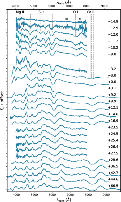
Figure 2: Observed spectral sequence of SN 2019yvq. Spectra have been normalized by their median flux between 7200 and 7400 Å. The phase of each observation relative to $T_{B,\mathrm{max}}$ is shown to the right of the individual spectra. Prominent spectral features from intermediate mass elements (IMEs) are highlighted with vertical-dashed lines. Some of the spectra show imperfect Telluric subtractions, giving rise to the non-smooth features around $\lambda_{\mathrm{obs}}\approx 7600$ Å. The blue and red edges of the $-12.9$ d spectrum are not shown for clarity.

With the exception of SEDM, all observations were obtained with the slit positioned along the parallactic angle, and the spectra were reduced using standard procedures in IDL/Python/Matlab. SEDM is a low-resolution ($R\approx 100$) integral field unit (Blagorodnova et al., 2018), and the observations are reduced using the custom pysedm software package (Rigault et al., 2019). While SEDM was designed specifically for SN classification (e.g., Fremling et al., 2020), the quality for SN 2019yvq is high enough to provide detailed absorption line measurements (see §5.2).

3 NGC 4441: The Host of SN 2019yvq

NGC 4441 is the host galaxy of SN 2019yvq. Sloan Digital Sky Survey (SDSS; York et al. 2000) spectroscopic measurements of the nucleus of NGC 4441 yield a heliocentric-recession velocity of 2663 km s^-1 ($z_{\mathrm{helio}}=0.00888$; Abolfathi et al. 2018) and a template-matched STARBURST classification for NGC 4441. Morphologically, NGC 4441 is classified as a peculiar, weakly barred, late-type lenticular galaxy (SABO$+$ pec; de Vaucouleurs et al. 1991). SDSS images show a clear dust lane near the center of the galaxy.

Using the 2M++ model of Carrick et al. (2015), we estimate a peculiar velocity toward NGC 4441 of $+328.6$ km s^-1, which combined with the recession velocity in the frame of the cosmic microwave background (CMB; $v_{\mathrm{CMB}}=2770.6$ km s^-1), yields a total recession velocity $=3099.2\pm 150$ km s^-1. The final uncertainty in the total recession velocity is dominated by systematic uncertainties in the 2M++ model. The 2M++ estimate is consistent, to within $\sim$5%, with the Virgo and Great Attractor infall models of Mould et al. (2000). Adopting $H_{0}=73$ km s^-1 Mpc^-1, we estimate the distance to NGC 4441 to be $42.5\pm 2.1$ Mpc, corresponding to a distance modulus of $\mu=33.14\pm 0.11$ mag, where the uncertainty on $\mu$ is dominated by the uncertainty in the peculiar velocity correction. We hereafter adopt $33.14\pm 0.11$ mag as the distance modulus to NGC 4441.

We estimate the total reddening toward SN 2019yvq to be small. There is relatively little line-of-sight extinction due to the Milky Way, $E(B-V)\approx 0.018$ mag (Schlegel et al., 1998; Schlafly & Finkbeiner, 2011). Furthermore, we do not find significant evidence for strong interstellar extinction in NGC 4441. Figure 3 highlights the Na I D absorption in the spectrum of SN 2019yvq due to gas in NGC 4441 and the Milky Way from our highest-resolution spectrum, $R\approx 4000$, obtained with Binospec+MMT. The Na I D absorption is weak, and we estimate a total equivalent width (EW) $=390$ mÅ for NGC 4441 and $220$ mÅ for the Milky Way. There is a systematic uncertainty of $\sim$10% on each of these estimates due to uncertainties in the continuum-fitting procedure.

Assuming similar properties for the dust in NGC 4441 and the Milky Way, we scale the color excess measurement for the Milky Way by the ratio of Na I D EWs to estimate $E(B-V)\approx 0.032$ mag for SN 2019yvq due to interstellar absorption in NGC 4441. This yields a total color excess toward SN 2019yvq of $E(B-V)\approx 0.05$ mag, which we adopt for the subsequent analysis in this study. We note that this estimate is consistent, to within the uncertainties, with the EW(Na I D)–$E(B-V)$ relations presented in Poznanski et al. (2012). Further support for low interstellar extinction toward SN 2019yvq is the lack of a detection of the K I $\lambda\lambda$7665, 7699 interstellar lines, or the diffuse interstellar band at 5780 Å, which also serve as proxies for extinction (Phillips et al., 2013).

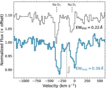
Figure 3: Zoom in on our moderate resolution ($R\approx 4000$) MMT+Binospec spectrum of SN 2019yvq highlighting absorption due to Na I D in the host galaxy, NGC 4441 (blue solid line), and the Milky Way (thin black line). The velocity scale is centered on the D₁ line in NGC 4441, with the SDSS redshift shown via the vertical-dashed line. The velocity scale is centered on 5895.92 Å for the Milky Way absorption lines. The Na I D lines, which serve as a proxy for interstellar dust-obscuration along the line of sight (e.g., Poznanski et al. 2012; Phillips et al. 2013) are weak, indicating a relatively small amount of reddening.

The measured redshift of the Na I D doublet in the Binospec spectrum is 0.0094. We adopt this, rather than the SDSS measurement of 0.00888, as the redshift of SN 2019yvq, $z_{\mathrm{SN}}$. This choice does not ultimately play a significant role in our final analysis, as our ejecta velocity measurements and rest-frame time differences would change by $<1\%$ when using $z_{\mathrm{SDSS}}$ versus our adopted $z_{\mathrm{SN}}$.

4 Photometric Analysis

4.1 The Time of First Light, $t_{\mathrm{fl}}$

We estimate the time of first light, $t_{\mathrm{fl}}$, for SN 2019yvq following the procedure described in Miller et al. (2020). Briefly, Miller et al. (2020) model the early emission from an SN Ia as a power law in time, $f\propto(t-t_{\mathrm{fl}})^{\alpha}$, where $f$ is the flux, $t$ is time, and $\alpha$ is the power-law index. $t_{\mathrm{fl}}$ is assumed to be the same everywhere in the optical, allowing us to simultaneously fit observations in each of the ZTF filters.

An important caveat for SN 2019yvq is that the observed early decline in the light curve clearly does not follow the simple power-law model, and thus these observations must be masked when performing the fit. We conservatively exclude observations from the first two nights of ZTF detection from the fit (this choice is conservative as it is unclear when the mechanism that powers the initial bump in SN 2019yvq no longer significantly contributes to the flux in the $g_{\mathrm{ZTF}}$ and $r_{\mathrm{ZTF}}$ filters). From the fit we find $t_{\mathrm{fl}}$$=-17.5^{+1.0}_{-1.3}$ d relative to $T_{B,\mathrm{max}}$. We know that the time of explosion must be $<-17.4$ d based on the discovery detection in Itagaki 2019, and, by definition $t_{\mathrm{fl}}\geq t_{\mathrm{exp}}$, meaning a portion of the posterior distribution for our model cannot be correct. We find $\alpha_{g}=2.15^{+0.49}_{-0.36}$ and $\alpha_{r}=1.91^{+0.42}_{-0.31}$, which are typical of the normal SNe Ia studied in Miller et al. (2020). If we only exclude the first observation from the model fit we find significantly different results with a rise time that increases by $\sim$5 d and power-law indices that increase by $\gtrsim 1$. We note that such a long rise is unlikely, however, as our spectroscopic models (see §5.1) estimate the time of explosion, $t_{\mathrm{exp}}$, to be $\sim$17.9 d prior to $T_{B,\mathrm{max}}$, fully consistent with our estimate of $t_{\mathrm{fl}}$.

4.2 Luminosity of the Initial UV/optical Flash

To estimate the luminosity and temperature of the initial UV/optical flash from SN 2019yvq, we model the broadband SED as a blackbody. The assumed distance and reddening toward SN 2019yvq are taken from §3. The ZTF optical and Swift UV observations were not simultaneous, so we interpolate the optical light curves to estimate the flux during the same epochs as Swift observations. While SNe Ia do not emit as pure blackbodies, our initial spectrum of SN 2019yvq shows a blue and nearly featureless continuum largely consistent with blackbody emission. The blackbody assumption is therefore reasonable for the early flash from SN 2019yvq, which is distinctly different from normal SNe.

Following interpolation to an epoch 1.24 d after $t_{\mathrm{fl}}$ ($\mathrm{MJD}=58$,846.93), and including the $uvw2$ filter, we estimate a blackbody luminosity $L=(1.7^{+0.2}_{-0.1})\times 10^{42}$ erg s^-1 and temperature $T_{\mathrm{eff}}=14.8^{+0.9}_{-1.2}$ kK. This estimate represents a lower limit to the peak luminosity of the initial flash, as the UV flux was already decreasing at this time (Swift obtained two sets of UV observations separated by $\sim$90 min during the first epoch of observations, and the $uvm2$ and $uvw1$ flux is clearly decreasing during this time; see Figure 1).

At an epoch 3.15 d after $t_{\mathrm{fl}}$, we estimate the luminosity and temperature to have fallen to $L=(7.0^{+0.9}_{-0.6})\times 10^{41}$ erg s^-1 and $T_{\mathrm{eff}}=8.7^{+0.5}_{-0.4}$ kK, respectively. For this epoch we have excluded the $uvw2$ flux from the blackbody model due to the significantly lower temperature, and known red leak for that filter (see §2.2). This measurement of $T_{\mathrm{eff}}$ is consistent with our model spectrum from 2.6 d after $t_{\mathrm{fl}}$ (see §5.1). At a similar epoch, $\sim$4 d after explosion, Cao et al. (2015) estimated a UV flash luminosity of $\sim$3$\times 10^{41}$erg s^-1 in iPTF 14atg, a factor of $\sim$2 less than for SN 2019yvq.

Finally, if we conservatively assume that the early flash peaked 1 d after $t_{\mathrm{fl}}$ (i.e., at the epoch of the first Swift observation), and abruptly ended 3 d after $t_{\mathrm{fl}}$ (i.e., at the epoch of the second Swift observation), then the initial flash emitted a total integrated energy of $\sim$4$\times 10^{42}$ erg. These assumed times are highly uncertain, however, it is likely that the SN exploded before $t_{\mathrm{fl}}$ (see, e.g., §5.1 and 6), and the UV flux continues to decline $>$3 d after $t_{\mathrm{fl}}$ (Figure 1) suggesting the flash lasted longer than 3 d.

4.3 Bolometric Luminosity, ⁵⁶Ni Mass, and Mass of the Ejecta

While the early emission from SN 2019yvq may be approximated as a blackbody, SNe Ia do not emit as blackbodies around maximum light. To estimate the bolometric luminosity of SN 2019yvq, we model changes in the observed flux in the $uvm2$, $uvw1$, $g_{\mathrm{ZTF}}$, $r_{\mathrm{ZTF}}$, and $i_{\mathrm{ZTF}}$ filters as a Gaussian process (Rasmussen & Williams, 2006) using the gaussian_process library in scikit-learn (Pedregosa et al., 2011). This allows us to interpolate flux measurements in each of these filters to a grid of times between 1 and 70 d after $t_{\mathrm{fl}}$, while also estimating an uncertainty on the interpolation. From there, we can estimate the bolometric luminosity, $L_{\mathrm{bol}}$, via trapezoidal integration of the SED.

There is emission blueward of the $uvm2$-band and redward of the $i_{\mathrm{ZTF}}$-band that is not constrained by our observations, and for fast-declining SNe the near-infrared (NIR) provides a significant contribution to $L_{\mathrm{bol}}$ (e.g., Taubenberger et al., 2008). To estimate the NIR flux, we extrapolate redward from the $i_{\mathrm{ZTF}}$-band to the $K_{s}$-band ($\lambda_{\mathrm{eff}}=2.159\,\mu$m) by assuming the $K_{s}$-band flux is equal to the ratio of the $i_{\mathrm{ZTF}}$-band to the $K_{s}$-band flux for a 8500 K blackbody. This choice of temperature is reasonable based on our TARDIS spectral models (see §5.1 and Table 4). While the true temperature is not constant, we find that varying the temperature between 6000 and 12,500 K changes the peak $L_{\mathrm{bol}}$ by $\lesssim\,3$%, which is significantly less than the total systematic uncertainty. The assumed emission redward of the $i_{\mathrm{ZTF}}$-band results in a NIR contribution of $\sim$20% to $L_{\mathrm{bol}}$ near maximum light, and $\sim$35% at $T_{B,\mathrm{max}}$ $\approx+30$ d. This is similar to SN 2004eo, an SN with an intermediate decline rate like SN 2019yvq (see §4.4), and other fast-declining SNe Ia (Taubenberger et al., 2008).

Similar to our procedure in the NIR, we estimate the flux in the far-UV by extrapolating between the $uvm2$-band and 1000 Å assuming a 12,500 K blackbody. While such a high temperature is only appropriate for the early UV flash from SN 2019yvq (see §4.2), the far-UV contribution to $L_{\mathrm{bol}}$ following this assumption is negligible ($\lesssim 1$%) around maximum light and later epochs.

In the near-UV, probed by the UVOT $uvm2$ and $uvw1$ filters, the SN is only marginally detected at epochs $>26.5$ d after $t_{\mathrm{fl}}$ (see Figure 1). Given the low S/N in the Swift observations at these epochs, for $t>t_{\mathrm{fl}}+26.5$ d we interpolate the $uvm2$ and $uvw1$ flux by assuming their ratio relative to the $g_{\mathrm{ZTF}}$ flux, which is measured at very high S/N, is fixed and set by their relative ratios at $t=t_{\mathrm{fl}}+26.5$ d. Fixing the UV flux in this manner does not change our estimate of the ⁵⁶Ni mass, and does not have a significant effect on our estimate of the total ejecta mass.

The bolometric luminosity of SN 2019yvq is shown as a function of time in Figure 4. Statistical uncertainties in $L_{\mathrm{bol}}$ are estimated via bootstrap resampling of the interpolated flux at each epoch, and are typically on the order of a few percent. We estimate a systematic uncertainty of $\sim$10% based on the total procedure (including interpolation, extrapolation, and integration).

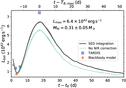
Figure 4: Bolometric luminosity, $L_{\mathrm{bol}}$, of SN 2019yvq as a function of time. $L_{\mathrm{bol}}$ is estimated via SED integration (see text) and shown as a black line, with statistical uncertainties shown in light gray. Purple squares show luminosity estimates from spectral modeling (see §5.1), orange circles show luminosity estimates from a blackbody fit to the SED (see §4.2). The methods generally agree, though the TARDIS spectral models likely overestimate the flux around maximum light (see text). The luminosity of SN 2019yvq assuming no NIR correction is shown as a dashed green line. The total inferred mass of synthesized ⁵⁶Ni is $0.31\pm 0.05\,M_{\odot}$.

As shown in Figure 4 the method compares favorably with a blackbody model (at early epochs) and spectroscopic modeling (during the SN rise). The maximum-light luminosity estimate from the TARDIS spectral model likely overestimates the flux in the NIR (see the third panel in Figure 7), due to the model assumption that there is a single, sharp photosphere that does not vary with wavelength. This explains the discrepancy between SED integration and the TARDIS model at that epoch.

From the SED integration we find that the bolometric luminosity of SN 2019yvq peaked 18.1 d after $t_{\mathrm{fl}}$ ($\sim$0.6 d after $T_{B,\mathrm{max}}$) at $L_{\mathrm{bol,max}}=6.4\pm 0.1\,(\mathrm{statistical})\pm 0.6\,(\mathrm{systematic})\times 10^{42}\,\mathrm{erg\,s}^{-1}$. This peak luminosity is $\sim$70% larger than the peak luminosity of iPTF 14atg ($3.8\times 10^{42}\,\mathrm{erg\,s}^{-1}$; Kromer et al., 2016).

From Arnett’s rule (Arnett, 1982), which states that the peak luminosity is equal to the instantaneous rate of radioactive energy released by ⁵⁶Ni, we estimate the total mass of ⁵⁶Ni, $M_{\mathrm{{}^{56}Ni}}$, synthesized in the explosion. Using Equation 19 from Nadyozhin (1994, see also ), we find $M_{\mathrm{{}^{56}Ni}}=0.31\pm 0.05\,M_{\odot}$, where the uncertainty is dominated by the (assumed) systematic uncertainty on $L_{\mathrm{bol}}$. We note that if our previous assumption about the NIR contribution to $L_{\mathrm{bol}}$ at maximum light is revised downward from $\sim$20% to $\sim$5%, as is typical for normal SNe Ia (e.g., Suntzeff, 1996; Contardo et al., 2000), the total ⁵⁶Ni mass still agrees with the above estimate to within the uncertainties. This yield is low for a normal SN Ia as typical explosions yield $\sim$0.4–0.8 $M_{\odot}$ of ⁵⁶Ni (e.g., Scalzo et al., 2014b).

Following Jeffery (1999), we can estimate the total mass ejected by SN 2019yvq, $M_{\mathrm{ej}}$, by calculating the transparency timescale, $t_{0}$, from the decline of the bolometric light curve (see also Stritzinger et al., 2006; Scalzo et al., 2014a; Dhawan et al., 2018). Briefly, $t_{0}$ is a parameter that governs the time-varying $\gamma$-ray optical depth of an SN, and it is related to $M_{\mathrm{ej}}$ as follows (Jeffery, 1999; Dhawan et al., 2018):

$$M_{\mathrm{ej}}=1.38\left(\frac{1/3}{q}\right)\left(\frac{v_{e}}{3000\,\mathrm{km\,s}^{-1}}\right)^{2}\left(\frac{t_{0}}{36.80\,\mathrm{d}}\right)^{2}M_{\odot},$$ (1)

where $v_{e}$ is the e-folding velocity of an exponential density profile, and $q$ is a form factor that describes the distribution of ⁵⁶Ni in the ejecta ($q=1/3$ corresponds to an evenly distributed ⁵⁶Ni profile). In Equation 1, the $\gamma$-ray opacity has been assumed to be 0.025 cm² g^-1.

For SN 2019yvq we estimate $t_{0}=42.0\pm 1.0$ d (the uncertainty is dominated by the uncertainty on the rise time, for which we adopt 1 d). Assuming $v_{e}=3000\pm 180$ km s^-1 and that $q=0.45\pm 0.08$, we find $M_{\mathrm{ej}}=1.33\pm 0.27\,M_{\odot}$. Unlike our estimate of $M_{\mathrm{{}^{56}Ni}}$, the adopted NIR correction does affect the measurement of $t_{0}$. In addition to the total luminosity, Figure 4 shows the SED-integrated luminosity assuming no NIR flux (i.e., $\mathrm{flux}=0$ for all $\lambda>1\,\mu$m). From this light curve we estimate $t_{0}=38.1\pm 1.0$ d, corresponding to $M_{\mathrm{ej}}=1.10\pm 0.22\,M_{\odot}$. Given the overall uncertainty in the NIR correction, our observations broadly bracket the total mass of ejecta to be somewhere between $\sim$0.9 and 1.5 $M_{\odot}$.

4.4 Maximum Light and Decline

While the rise time and power-law indices of SN 2019yvq are similar to other normal SNe Ia (see §4.1), the full photometric evolution does not resemble a normal SN Ia. The photometric evolution of SN 2019yvq is highlighted in Figure 5, where SN 2019yvq is compared to 121 normal SNe Ia from Yao et al. (2019). SN 2019yvq is somewhat underluminous ($M_{g,\mathrm{max}}\approx-18.5$ mag), declines rapidly [$\Delta m_{15}(g)=1.30^{+0.01}_{-0.02}$ mag, uncertainties represent the 68% credible region], and does not exhibit a “shoulder” in the $r_{\mathrm{ZTF}}$ or a strong secondary maximum in the $i_{\mathrm{ZTF}}$ light curves post maximum. The slightly underluminous peak and moderately fast decline of SN 2019yvq are very similar to SN 1986G-like SNe Ia, which represent a transitional group between normal SNe Ia and the underluminous SN 1991bg-like class (e.g., Taubenberger 2017 and references therein). While the photometric evolution of SN 2019yvq is similar to 86G-like SNe, we show that SN 2019yvq is spectroscopically distinct from these transitional SNe (§5.3).

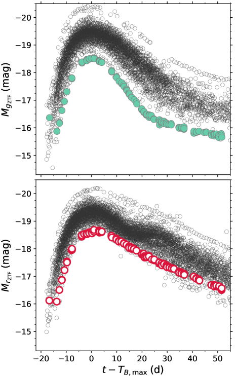
Figure 5: Photometric evolution of SN 2019yvq compared to 121 normal SNe Ia observed by ZTF (Yao et al., 2019) in the $g_{\mathrm{ZTF}}$ (top) and $r_{\mathrm{ZTF}}$ (bottom) filters. The normal SNe are shown as open gray circles, while the symbols for SN 2019yvq are the same as Figure 1. Relative to normal SNe Ia, SN 2019yvq is fainter, declines faster in $g_{\mathrm{ZTF}}$, and lacks the “shoulder” typically seen in the $r_{\mathrm{ZTF}}$ filter. Normal SNe light curves have been corrected for host-galaxy reddening and $K$-corrections have been applied, with both determined via SNooPY (see Bulla et al. 2020 for details of our implementation). $K$-corrections have not been applied to the light curve of SN 2019yvq.

We also find that standard SN Ia fitting techniques do not provide good matches to the evolution of SN 2019yvq. For example, a SNooPY (Burns et al., 2011) fit to the optical light curve requires significant host-galaxy extinction [$E(B-V)_{\mathrm{host}}\approx 0.4$ mag, see §3] to match the observed red colors, while predicting a secondary maximum in the $i_{\mathrm{ZTF}}$-band and a fast evolution after peak that is not seen in SN 2019yvq. A SALT2 (Guy et al., 2007) fit leads to similar inconsistencies to those in SNooPy. These inconsistencies support our conclusion above that the photometric evolution of SN 2019yvq does not match normal SNe Ia.

4.5 Color Evolution

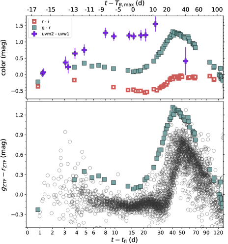
Figure 6: Photometric color evolution of SN 2019yvq relative to $t_{\mathrm{fl}}$ (the timescale relative to $T_{B,\mathrm{max}}$ shown along the top axis only applies to SN 2019yvq). Bottom: $g_{\mathrm{ZTF}}$$-$$r_{\mathrm{ZTF}}$ evolution of SN 2019yvq (solid green squares), corrected for the total interstellar extinction (see §3), and compared with the evolution of 62 normal SNe Ia (open circles) observed within 5 d of $t_{\mathrm{fl}}$ by ZTF (from Bulla et al. 2020). SN 2019yvq is the reddest SN in the group, and it exhibits the fastest evolution to red colors post-$T_{B,\mathrm{max}}$. Top: the $uvm2-uvw1$ (purple crosses), $g_{\mathrm{ZTF}}$$-$$r_{\mathrm{ZTF}}$ (solid, green squares), and $r_{\mathrm{ZTF}}$$-$$i_{\mathrm{ZTF}}$ (open, red squares) color evolution of SN 2019yvq.

SN 2019yvq is further distinguished from normal SNe Ia by its unusual color evolution (Figure 6). The lower panel of Figure 6 shows the $g_{\mathrm{ZTF}}$$-$$r_{\mathrm{ZTF}}$ evolution of 62 spectroscopically normal SNe Ia with ZTF observations within 5 d of $t_{\mathrm{fl}}$ (see Bulla et al. 2020), with the color evolution of SN 2019yvq over-plotted. The initially blue colors in SN 2019yvq rapidly evolve to the red over the first few days of observation before gradually becoming bluer in the time leading up to $T_{B,\mathrm{max}}$ (this behavior is deemed an early “red bump” in Bulla et al. 2020). Similar red bumps are only seen in 6 of the 62 normal SNe Ia ($\sim$10%) in the ZTF sample (Bulla et al., 2020), and they are typically less pronounced than what is observed in SN 2019yvq.

Furthermore, while normal SNe Ia exhibit a large scatter in $g_{\mathrm{ZTF}}$$-$$r_{\mathrm{ZTF}}$ shortly after $t_{\mathrm{fl}}$ they evolve to form a tight locus between $\sim$10 and 30 d after $t_{\mathrm{fl}}$. SN 2019yvq is redder at peak than each of the normal SNe Ia in the Bulla et al. (2020) sample. Post maximum, only one normal SN Ia, ZTF 18abeegsl (SN 2018eag), exhibits a similarly rapid decline in $g_{\mathrm{ZTF}}$$-$$r_{\mathrm{ZTF}}$ color. The $g_{\mathrm{ZTF}}$$-$$r_{\mathrm{ZTF}}$ color evolution of SN 2019yvq is again intermediate between normal SNe Ia and underluminous 91bg-like SNe. Figure 6 shows that normal SNe Ia are reddest at $\sim$+30 d, while 91bg-like SNe are reddest between $\sim$+10 and 15 d (Burns et al., 2014). SN 2019yvq reaches a $g_{\mathrm{ZTF}}$$-$$r_{\mathrm{ZTF}}$ maximum at an intermediate time of $\sim$+20 d.

The offset in the $g_{\mathrm{ZTF}}$$-$$r_{\mathrm{ZTF}}$ color evolution of SN 2019yvq relative to normal SNe Ia would be reduced if the reddening toward SN 2019yvq has been significantly underestimated. A color excess of $E(B-V)\approx 0.25$ mag, rather than the 0.05 mag adopted in §3, would roughly align the $g_{\mathrm{ZTF}}$$-$$r_{\mathrm{ZTF}}$ color of SN 2019yvq with the tight locus between $\sim$5 and 20 d after $t_{\mathrm{fl}}$ seen in Figure 6. Such a correction would also bring the peak optical brightness of SN 2019yvq in line with normal SNe Ia [for $E(B-V)\approx 0.25$ mag, $M_{g}\approx-19.25$ mag and $M_{r}\approx-19.1$ mag for SN 2019yvq].

While the spectral appearance of SN 2019yvq is similar to some normal SNe Ia (see §5.3), the observed rapid decline in the $g_{\mathrm{ZTF}}$ filter provides strong evidence that SN 2019yvq is not a normal luminosity SN Ia. Phillips (1993) showed that in the optical SNe Ia follow a brightness–width relation, whereby brighter explosions decline less rapidly. Thus, with a typical peak in the optical, as would be implied with $E(B-V)\approx 0.25$ mag, the fast decline in SN 2019yvq [$\Delta m_{15}(g)=1.3$ mag] would be largely unprecedented. This conclusion is further corroborated by the rapid evolution of the $g_{\mathrm{ZTF}}$$-$$r_{\mathrm{ZTF}}$ color to the red after $T_{B,\mathrm{max}}$ and the lack of a secondary maximum in the $i_{\mathrm{ZTF}}$-band, each of which is typical of lower luminosity SNe Ia (see Taubenberger, 2017, and references therein). We therefore conclude that the color excess toward SN 2019yvq is not underestimated, and that the SN is instead intrinsically red in the optical.

Even if one ignores the striking initial bump in the light curve of SN 2019yvq, we can still conclude that SN 2019yvq is not a normal SN Ia based on its other photometric properties (e.g., relatively faint peak optical brightness, moderately fast decline, lack of a NIR secondary maximum, and red appearance at peak).

5 Spectral Evolution of SN 2019yvq

Optical spectra of SN 2019yvq were obtained at phases from $-$14.9 d (2.6 d after $t_{\mathrm{fl}}$) to 66.5 d after $T_{B,\mathrm{max}}$. Details of the spectra are presented in Table 3 and the spectral evolution is shown in Figure 2. The absorption features in SN 2019yvq are typical of SNe Ia, including IMEs, primarily Si, Ca, and O, as well as iron-group elements (IGEs).

Table 4: TARDIS input parameters

Date	MJD	Phase	$t-t_{\mathrm{exp}}$	$L$	$v_{\mathrm{boundary}}$	$T_{\mathrm{boundary}}$
(UT)		(d)	(d)	($\log L_{\odot}$)	(km s-1)	(K)
2019 Dec 31.277	58,848.277	$-14.9$	3.0	8.55	25,000	8173
2020 Jan 03.217	58,851.217	$-12.0$	6.0	8.60	16,500	7925
2020 Jan 15.392	58,863.392	$+0.0$	18.0	9.29	10,500	9696

Note. — Phase is measured in rest-frame days relative to $T_{B,\mathrm{max}}$. The time of explosion, $t_{\mathrm{exp}}$, is assumed to be 0.4 d before $t_{\mathrm{fl}}$ for the TARDIS model.

5.1 TARDIS Models

To determine the structure of the ejecta and relative contributions of different ions at early and maximum-light phases, we have modeled the spectra at $-$14.9, $-12.0$, and $+$0.0 d using the one-dimensional (1D) Monte Carlo radiative transfer code TARDIS (Kerzendorf & Sim, 2014). We note that TARDIS assumes a single, sharp photosphere between the optically thick and thin regions. Therefore, if there is a contribution to the spectrum from an underlying quasi-blackbody (at early times this could be due to interaction, for example; see §6.1), this will impact the ability of TARDIS to fully reproduce the observations. Nevertheless, our models should provide a reasonable approximation of the plasma state within the ejecta. The parameters of our TARDIS models are given in Table 4.

The first spectrum of SN 2019yvq at $-$14.9 d (2.6 d after $t_{\mathrm{fl}}$, 3.0 d after the TARDIS-inferred $t_{\mathrm{exp}}$) shows shallow features consistent with IMEs moving at extremely high velocities ($>$ 20,000 km s^-1, Figure 2). The best-fitting TARDIS model is shown in Figure 7, along with the contribution of individual elements to the spectral features. For this model, we have assumed a uniform composition of O, Mg, Si, and S. Our model demonstrates that the shallow absorption features observed at this phase can be reproduced solely by IMEs (predominantly Si II), and that the presence of IGE is not required to match the data. Our model also confirms the high velocities of the ejecta – we find the spectral features and temperature are best reproduced with a photospheric velocity of $\sim$25,000 km s^-1.

Similarly, for the $-12.0$ d spectrum we find that a model that does not contain IGE above $\sim$16,500 km s^-1 reproduces the majority of the spectroscopic features. Again, our model contains a uniform composition of O, Mg, Si, and S, and is shown in Figure 7. At this phase the model suggests the photospheric temperature has not significantly changed, however, the features have become much more prominent. Compared to modeling of the spectroscopically similar SN 2002bo (see §5.3) at the same epoch (Stehle et al., 2005), we find SN 2019yvq has a lower photospheric temperature ($\sim$8000 K, compared to $\sim$9500 K for SN 2002bo).

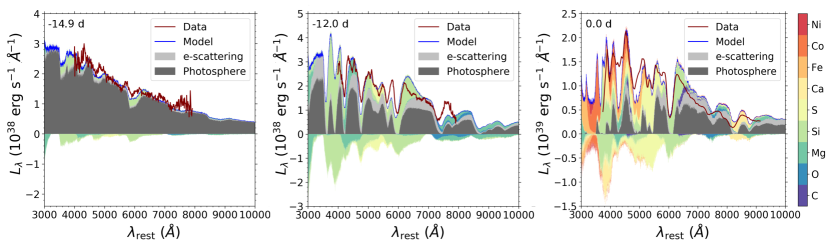
Figure 7: Comparison of TARDIS models to SN 2019yvq at $-$14.9 d (left), $-12.0$ d (middle), and $+$0.0 d (right), relative to $T_{B,\mathrm{max}}$. For each model, we color code a histogram showing the contribution of each element to the spectroscopic features, based on the last element with which a Monte Carlo photon packet experienced an interaction. Photon packets may be absorbed and re-emitted at different wavelengths, with the exception of those packets that only experience electron scattering. During electron scattering, only the direction of propagation is changed. These packets are shown in light gray. Photon packets that did not interact during the simulation are shown in dark gray. Contributions below and above zero show the SED of packets before and after their last line interaction. Note that non-interacting (photosphere) and e-scattering photon packets are not shown below zero.

While the early spectra of SN 2019yvq are dominated by IMEs, there is no evidence in the observed spectra for C II absorption. However, in our TARDIS models even if we increase the C abundance in the outer ejecta to large amounts (50%), the model spectra still lack any significant C II features at the time of our observations. Our ability to detect C II in the spectra of SN 2019yvq is likely affected by the extremely high ejecta velocities, which leads to blending with Si II. Therefore, despite the lack of a C II detection in the observed spectra, we are unable to place meaningful constraints on the C abundance in the very outermost ejecta.

Given that our $+0$ d maximum-light spectrum occurs 12 d after our previous model spectrum, we assume a composition for the inner ejecta ($\textless$ 16,500 km s^-1) similar to that found for SN 2002bo (Stehle et al., 2005). A more detailed ejecta structure could be achieved through modeling additional pre-maximum spectra, but is beyond the scope of the work presented here. As shown in Figure 7, our model is able to broadly reproduce many of the features observed. Notable exceptions include the features around $\sim$4200 and 4900 Å, which we attribute to Fe. Better spectroscopic agreement could potentially be achieved if SN 2019yvq had a lower abundance of IGE within the inner ejecta relative to SN 2002bo.

Overall, our TARDIS modeling demonstrates that SN 2019yvq is consistent with a low (or zero) fraction of IGE in the outer ejecta (i.e., there is little mixing in the SN ejecta). Additionally, the earliest phases show little change in temperature (see Table 4), as expected from the color evolution.

5.2 Si II Evolution

We have measured the velocity of the Si II $\lambda$6355 absorption feature following the procedure in Maguire et al. (2014, see their Section 2.5). We have also estimated the pseudo-equivalent widths (pEWs) of the Si II $\lambda\lambda$5972, 6355 features, allowing us to measure their ratio, also known as $\mathcal{R}($Si II$)$; see Hachinger et al. (2008) for the updated definition relative to Nugent et al. (1995).

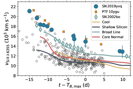
Figure 8: Velocity evolution of Si II $\lambda$6355 absorption in SN 2019yvq (large, filled circles). For comparison we also show the measurements for 264 SNe Ia observed by PTF (data from Maguire et al., 2014) as open circles, with SN 2010jn (PTF 10ygu), the SN with the fastest moving ejecta in the PTF sample, highlighted via orange crosses. We additionally show the velocity evolution of SN 2002bo (data from Benetti et al., 2004), an SN that is very similar to SN 2019yvq, as open diamonds. The median velocity evolution of each of the spectroscopic classes defined by Branch et al. (2006, Shallow Silicon, Core Normal, Broad Line, and Cool) are shown via solid lines. It is clear that SN 2019yvq has exceptionally high-velocity ejecta.

The velocity evolution of Si II $\lambda$6355 is shown in Figure 8, compared to measurements for the Palomar Transient Factory (PTF) SN Ia sample from Maguire et al. (2014) and the median velocity evolution of SNe Ia belonging to the four different classes (Shallow Silicon, Core Normal, Broad Line, and Cool) identified in Branch et al. (2006); hereafter, the Branch class. The Si II $\lambda$6355 velocity in SN 2019yvq is $\sim$15,000 km s^-1 around $T_{B,\mathrm{max}}$.

At $T_{B,\mathrm{max}}$, the pEW measurements for the Si II $\lambda$6355 and $\lambda$5972 features are $183\pm 1$ Å, and $13\pm 2$ Å, respectively, unambiguously classifying SN 2019yvq as a Branch Broad Line SN Ia. SN 2019yvq stands out in Figure 8 with some of the highest Si II velocities that have ever been observed. Within the PTF sample, only SN 2010jn (PTF 10ygu) exhibits a Si II absorption velocity as high as SN 2019yvq at every phase in its evolution. Furthermore, we also find that the Ca II infrared triplet (IRT) velocities are high (we first detect this feature in the $-3.0$ d SEDM spectrum; see Table 3), with a photospheric component velocity of $\sim$13,200 km s^-1 and a clear high-velocity component at $\sim$23,500 km s^-1. Within the PTF sample only one other SN (PTF 09dnp) has a Ca II high-velocity component with a similarly large velocity at the same phase.

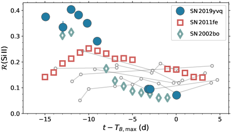
Figure 9: Evolution of the ratio of the pEW of Si II $\lambda$5972 to Si II $\lambda$6355, $\mathcal{R}($Si II$)$, in SN 2019yvq (large, filled circles). SN 2002bo (data from Benetti et al., 2004) and SN 2011fe (data from Pereira et al., 2013) are also highlighted as open diamonds and open squares, respectively. For comparison we also show the $\mathcal{R}($Si II$)$ evolution for five PTF SNe Ia (10mwb, 10qjq, 10tce, 10wof, 11hub) with $>3$ measurements over a duration $>8$ d (data from Maguire et al. 2014) and SN 2017erp (data from Brown et al., 2019) as connected, open circles. SN 2019yvq and SN 2002bo exhibit an unusual inversion in $\mathcal{R}($Si II$)$ as they evolve toward maximum light.

As first noted by Nugent et al. (1995), and later confirmed by Hachinger et al. (2008), $\mathcal{R}($Si II$)$ is a luminosity indicator, with larger values of $\mathcal{R}($Si II$)$ corresponding to lower luminosities. This correlation is driven by the ionization balance of Si II/Si III, with cooler objects having stronger Si II $\lambda$5972 features. In Figure 9 we show the evolution of $\mathcal{R}($Si II$)$ as a function of time for SN 2019yvq, compared to SN 2011fe, SN 2002bo, SN 2017erp, and five SNe with multiple measurements over a long baseline from the PTF SN Ia spectral sample. Figure 9 shows that most SNe Ia have a relatively flat evolution in $\mathcal{R}($Si II$)$ in the time leading up to $T_{B,\mathrm{max}}$ (see also Riess et al., 1998). SN 2019yvq and SN 2002bo, however, feature a very different evolution with initially large values of $\mathcal{R}($Si II$)$ that rapidly decrease to very low values between $\sim$10 and $\sim$5 d before $T_{B,\mathrm{max}}$.

At face value, the $\mathcal{R}($Si II$)$ evolution in Figure 9 suggests that the effective temperature of SN 2019yvq increases significantly as it rises to maximum light. Both the optical colors, which become bluer in the $\sim$14 d leading up to $T_{B,\mathrm{max}}$ (see Figure 6), and the TARDIS modeling (see Table 4) confirm an increase in temperature over the period in which $\mathcal{R}($Si II$)$ decreases. While the UV $-$ optical colors become redder over the same time period, this is likely due to the increasing IGE fraction, and hence increased UV blanketing, as the photosphere recedes (see §5.1), and not a decrease in temperature.

This behavior is similar to, though less extreme than, SN 2002bo, which increases in temperature from $\sim$9,500 K at $-12.9$ d to $\sim$14,000 K at maximum light (Stehle et al., 2005). The maximum-light temperature of SN 2002bo is similar to Branch Core Normal SNe, such as SN 2011fe, which typically have temperatures of $\sim$14,500–15,000 K at maximum light (Mazzali et al., 2014).

Benetti et al. (2004) interpreted these competing effects as the result of significant Si II mixing in the ejecta of SN 2002bo. Mixing or synthesized Si in the outermost layers of the ejecta would (i) lead to larger Si II velocities, (ii) produce Si II line ratios that indicate cool temperatures (because there is less radioactive material to heat the ejecta), before eventually (iii) producing low values of $\mathcal{R}($Si II$)$ as the photosphere recedes through the ejecta to higher temperature regions. This picture is consistent with the Stehle et al. (2005) models of SN 2002bo. In those models, Si completely dominates the species at velocities above $\sim$23,000 km s^-1, while there is very little ($\sim$1%) IGE above 1.35 $M_{\odot}$ in radial mass coordinates. A similar physical scenario likely explains the changes in Si II absorption seen in SN 2019yvq. Although the temperature change in SN 2019yvq is less dramatic than in SN 2002bo, this may reflect slight differences in the ejecta composition as we find SN 2019yvq is consistent with no IGEs in the outer layers of the SN ejecta.

5.3 Spectral Comparison

In Figure 10, we compare the spectral evolution of SN 2019yvq to two Branch Broad Line SNe Ia, SN 2002bo and SN 2010jn, and two Branch Cool SNe Ia, SN 1986G and SN 2004eo (Cristiani et al., 1992; Benetti et al., 2004; Pastorello et al., 2007; Silverman et al., 2011; Hachinger et al., 2013; Maguire et al., 2014) at four phases, pre-maximum, maximum, $\sim$1 week post maximum, and $\sim$6 weeks post maximum. The evolution of SN 2019yvq and SN 2002bo is remarkably similar at all phases. The only significant difference between the two is the absorption trough at $\sim$4800 Å in the pre-maximum and maximum-light spectra. This feature, which is typically attributed to a combination of Fe II, Fe III, and Si II, is extremely narrow in SN 2019yvq. This is in agreement with the TARDIS modeling results where no Fe is required in the outer ejecta of SN 2019yvq to match the observed spectra at early times. SN 2010jn, which exhibits large Si II velocities like SN 2019yvq, shows weaker IME absorption and stronger IGE absorption than SN 2019yvq. While the Branch Cool SNe 1986G and 2004eo show lower velocities than SN 2019yvq, there is strong agreement in the relative Si II line strengths of SN 1986G and the earliest spectra of SN 2019yvq.

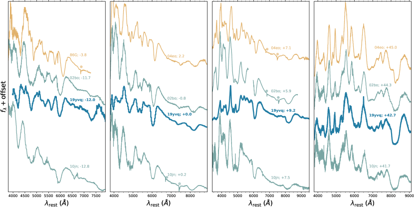
Figure 10: Spectral comparison of SN 2019yvq to Branch Broad Line and Cool SNe Ia. All spectra have been corrected for the total line-of-sight extinction with adopted $E(B-V)$ values of 0.9, 0.38, 0.39, 0.109, and 0.05 mag for SNe 1986G (Phillips et al., 1987), 2002bo (Stehle et al., 2005), 2010jn (Hachinger et al., 2013), 2004eo (Pastorello et al., 2007), and SN 2019yvq (this work), respectively. Left panel: pre-maximum spectra showing the similarity of SN 2019yvq and SN 2002bo. While the expansion velocities in the Cool SN 1986G spectrum are considerably lower than those in the Broad Line SNe, the relative ratios of the Si II features are similar to SN 2019yvq. Second panel: Comparison of SN 2019yvq to the Broad Line SNe 2002bo and SN 2010jn. These SNe all feature nearly identical maximum-light spectra. By this phase, the relative strength of the Si II absorption features is no longer similar to Branch Cool SNe, as illustrated by SN 2004eo. Third panel: $\sim$1 week post-maximum spectra. Fourth panel: Transitional phase spectra. Comparison spectra have been downloaded from WISeREP (Yaron & Gal-Yam, 2012), with spectra for individual SNe from the following sources: SN 1986G (Cristiani et al., 1992), SN 2002bo (Benetti et al., 2004; Silverman et al., 2011), SN 2010jn (PTF 10ygu) (Hachinger et al., 2013; Maguire et al., 2014), SN 2004eo (Pastorello et al., 2007).

The maximum-light spectra shown in the second panel of Figure 10 reveal a higher temperature for SN 2019yvq, as the Si II $\lambda$5972 absorption has nearly disappeared around $T_{B,\mathrm{max}}$ [see discussion of $\mathcal{R}($Si II$)$ in §5.2]. This increase in temperature is consistent with the change in optical colors (Figure 6) and TARDIS spectral modeling (§5.1). The appearance of SN 2019yvq, SN 2002bo, and SN 2010jn are all similar at this epoch, with the exception of the 4800 Å feature mentioned above. SN 2004eo has a similar appearance to SN 2019yvq, though it has lower velocities and cooler temperatures (as traced by Si II $\lambda$5972).

The $+9.2$ d spectrum of SN 2019yvq, shown in the third panel of Figure 10, shows absorption due to IGE. Additional differences between SN 2019yvq and SN 2002bo can be seen at this phase. There is stronger absorption in SN 2019yvq blueward of Ca II H&K, and the S II “W” absorption feature is still present in SN 2019yvq and it cannot be identified in SN 2002bo or SN 2010jn. SN 2004eo maintains an appearance that is somewhat similar to SN 2019yvq, though as before, the temperature [as indicated by $\mathcal{R}($Si II$)$] and velocities are lower.

Spectra obtained $\sim$6 weeks after maximum light are shown in the fourth panel of Figure 10. By this time, as the SNe are transitioning into a nebular phase, the appearance of each spectrum is similar modulo some minor differences in the relative line strengths of different features.

6 A Physical Explanation for SN 2019yvq

The most striking feature of SN 2019yvq is the observed UV/optical peak that occurs shortly after discovery (Figure 1). Any model to explain SN 2019yvq must account for this highly unusual feature. A UV decline in the early phase of an SN Ia has previously only been observed in a single event, iPTF 14atg (Cao et al., 2015). Like SN 2019yvq, iPTF 14atg was a peculiar SN Ia, though it did not resemble SN 2019yvq in its peculiarity (iPTF 14atg exhibited low expansion velocities, and the spectra resembled SN 2002es; Ganeshalingam et al. 2012; Cao et al. 2015). Clearly resolved “bumps” in the early optical emission of SNe Ia are also rare, having only been seen in a few events: SN 2014J (Goobar et al., 2015), MUSSES1604D (Jiang et al., 2017), SN 2017cbv (Hosseinzadeh et al., 2017) and SN 2018oh (Dimitriadis et al., 2019; Shappee et al., 2019).

SN 2019yvq features other properties, in addition to an initial peak $\sim$17 d prior to $T_{B,\mathrm{max}}$, that separate it from normal SNe Ia. A good model should be able to explain the following:

1. The early UV/optical “flash” (Figure 1).

2. The moderately faint luminosity at peak (§4.3).

3. The relatively fast optical decline (§4.4).

4. The red optical colors at all epochs (Figure 6).

5. The lack of IGE in the early spectra (§5.1).

6. The evolution in $\mathcal{R}($Si II$)$ (§5.2 and Figure 9).

7. The high Si II velocities (Figure 8).

The moderately faint peak combined with the high Si II velocity is particularly rare (see, e.g., Figure 11 in Polin et al. 2019a, where SN 2019yvq would be well isolated from all the other SNe Ia).

As noted in §4.4, the photometric evolution of SN 2019yvq is similar to intermediate 86G-like SNe, however, the spectra feature much weaker Si II $\lambda$5972 absorption and larger expansion velocities than what is seen in 86G-like SNe (see Figure 10). Similarly, while the spectral appearance and evolution of SN 2019yvq is similar to SN 2002bo, and other Branch Broad Line SNe, the photometric properties are entirely different. SN 2002bo features a relatively slow decline [$\Delta{m}_{15}(B)=1.13$ mag, which corresponds to $\Delta{m}_{15}(g)\approx 0.8$ mag (see, e.g., Figure 2 in Folatelli et al., 2010)] with a clear secondary maximum in the $I$-band (Benetti et al., 2004), which stands in contrast to moderately fast decline [$\Delta{m}_{15}(g)=1.3$ mag, roughly $\Delta{m}_{15}(B)\approx 1.55$ mag (Folatelli et al., 2010)], and lack of $i_{\mathrm{ZTF}}$ secondary maximum in SN 2019yvq.

If we otherwise ignore the early flash, several of the remaining features (2–6) in the list above can be understood if the explosion that gave rise to SN 2019yvq produced a relatively small amount of ⁵⁶Ni (§4.3) that is confined to the inner regions of the SN ejecta. A low ⁵⁶Ni yield could explain the underluminous light curve and red colors, while a centrally concentrated IGE distribution could explain the IME-dominated early spectra, as the IGE would not have been mixed to these outer layers. Furthermore, with a centrally compact IGE ejecta composition, the photosphere would transition somewhat rapidly from ⁵⁶Ni poor to ⁵⁶Ni rich, resulting in a significant change in the temperature of the ejecta along the lines of what we see in the evolution of $\mathcal{R}($Si II$)$.

This interpretation is supported by photometric modeling of the rise of SN 2019yvq. Magee et al. (2020) developed a suite of models featuring different ⁵⁶Ni structures within the SN ejecta. These models were compared to early observations of SNe Ia to see which ones replicate what is observed in nature. Generally, it is found that centrally concentrated ⁵⁶Ni models do not match the early evolution of normal SNe Ia (Magee et al., 2020). Using the methods described in Magee et al. (2020), we have modeled the post-flash rise of SN 2019yvq using a new model with $M_{{}^{56}Ni}=0.3\,M_{\odot}$ (the models in Magee et al., 2020, all have $M_{{}^{56}Ni}>0.4\,M_{\odot}$ and are therefore more luminous than SN 2019yvq). After excluding the first two epochs of ZTF observations, as we consider the mechanism that produces the early UV flash to be different from the standard ⁵⁶Ni decay that powers most SNe Ia, we find that SN 2019yvq is best matched with compact ⁵⁶Ni distributions (following the convention of Magee et al., 2020, an EXP_Ni0.3_KE1.40_P21 model provides the best match to SN 2019yvq, see also Figure 12). We note, however, that Magee et al. (2020) demonstrate that the time of first detection can dramatically alter the inferred model properties and it is unclear which epochs (if any) should be excluded. Nevertheless, a scenario in which the ⁵⁶Ni and other IGEs are confined to the central regions of the ejecta is also consistent with our spectroscopic analysis (see §5.1).

On their own, a low-⁵⁶Ni yield that is centrally concentrated fails to explain the blue UV/optical flash seen in SN 2019yvq. A large number of scenarios have been proposed to explain early “bumps” or “flashes” in SN Ia light curves, including: shock cooling following the shock breakout from the surface of the WD (e.g., Piro et al. 2010; Rabinak & Waxman 2011), interaction between the SN ejecta and a nondegenerate binary companion (Kasen, 2010), extended clumps of ⁵⁶Ni in the SN ejecta (e.g., Dimitriadis et al. 2019; Shappee et al. 2019), double-detonation explosions (e.g., Noebauer et al. 2017; Polin et al. 2019a), and interaction between the SN ejecta and circumstellar material (e.g., Dessart et al. 2014; Piro & Morozova 2016; Levanon & Soker 2017).

Below we discuss each of these models, aside from the shock breakout model, and their ability to replicate observations of SN 2019yvq. We do not discuss shock breakout models as our initial detection of SN 2019yvq occurred at $M_{g}\approx-16.3$ mag. A progenitor radius of $\sim$10$\,R_{\odot}$ is needed to explain such a high luminosity (Piro et al., 2010; Rabinak & Waxman, 2011), which we consider implausible for a WD.

6.1 Companion Interaction

For SD progenitors of SNe Ia, the SN ejecta will shock on the surface of the nondegenerate companion giving rise to a short-lived transient in the days after explosion. Kasen (2010) provided models for the appearance of this interaction, which is primarily dependent upon the binary separation of the system (assuming Roche lobe overflow for the nondegenerate companion). The observed emission following the ejecta-companion collision is dependent upon the orientation of the binary system relative to the line of sight (Kasen, 2010).

An analytic formulation for the luminosity and effective temperature of the emission from the companion shock is given in Equations (22) and (25) in Kasen (2010). Brown et al. (2012) provide an analytic function to approximate the fractional decrease in the observed flux as a function of the orientation of the system. We combine the equations from Kasen (2010) and Brown et al. (2012) to model the early emission from SN 2019yvq as an ejecta-companion collision. We assume the interaction emits as a blackbody, and that the electron scattering opacity $\kappa_{e}=0.2$ cm² g^-1 (as in Kasen 2010). Assuming $z_{\mathrm{SN}}=0.0094$, $E(B-V)_{\mathrm{MW}}=0.018$ mag, and $E(B-V)_{\mathrm{host}}=0.032$ mag, we compare observed flux measurements with those predicted by the Kasen (2010) model at epochs with MJD$\,<58$,849.2 (i.e., the first $\sim$2.5 d after discovery when emission from the companion interaction is significantly brighter than the luminosity due to radioactive decay). The model parameters, summarized in Table 5, are constrained via a Gaussian likelihood and flat priors using an affine-invariant (Goodman & Weare, 2010) Markov Chain Monte Carlo (MCMC) ensemble sampler (Foreman-Mackey et al., 2013).

Table 5: Model Parameters $\Theta$ and Their Priors and Posteriors

$\Theta$	Description	Prior	Posterior
$a$	Companion separation	$\mathcal{U}(10^{10},10^{13})$	$9.1\pm 0.7\times 10^{11}$ cm
$M_{\mathrm{ej}}$	Ejecta mass	$\mathcal{U}(0.6,1.5)$	$1.1\pm 0.3\,M_{\odot}$
$v_{\mathrm{ej}}$	Ejecta velocity	$\mathcal{U}(5\times 10^{8},3\times 10^{9})$	$2.2\pm^{0.5}_{0.3}\times 10^{9}$ cm s-1
$\theta_{\mathrm{obs}}$	Binary viewing angle	$\mathcal{U}(0,180)$	$40\pm 28^{\circ}$
$t_{\mathrm{exp}}$	Time of explosion	$\mathcal{U}(t_{0}-5,t_{0})$	$58,845.82\pm 0.04$ (MJD)

Note. — Marginalized 1D posterior values represent the 68% credible region. $M_{\mathrm{ej}}$ is largely unconstrained by the observations. The posterior distribution on $\theta_{\mathrm{obs}}$ is effectively flat between $0^{\circ}$ and $\sim$70^∘, and $\sim$0 for all angles above $\sim$85^∘. There is a strong covariance between $a$ and $t_{\mathrm{exp}}$ and also between $v_{\mathrm{ej}}$ and $\theta_{\mathrm{obs}}$.

The results of this procedure are shown in Figure 11, where it is clear that the model presented in Kasen (2010) does an adequate job of explaining the early UV/optical emission from SN 2019yvq (constraints on the model parameters are reported in Table 5).

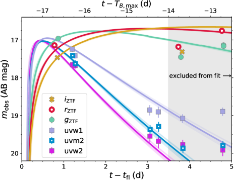
Figure 11: SN ejecta-companion-interaction models compared with the UV/optical observations of SN 2019yvq. Observation symbols are the same as Figure 1 (solid magenta squares show Swift $uvw2$ observations that are not shown in Figure 1). Solid lines show companion-interaction model predictions in each filter (the lines have the same colors as the corresponding symbols for each passband). The maximum a posteriori model is shown via the single bold lines, while other random draws from the posterior are shown as thin transparent lines. The shaded area shows observations that are excluded from the model fit. The overprediction of the optical flux $\sim$13.7 d prior to $T_{B,\mathrm{max}}$ suggests that companion interaction does not explain the early flash in SN 2019yvq (see text).

While the interaction models roughly approximate the SN emission in the $\sim$3 d after explosion, they significantly overestimate the flux immediately after the fitting window as shown in Figure 11. This problem is exacerbated by the fact that the models do not include emission associated with radioactive decay, meaning the true discrepancy between what is predicted and what is observed is even larger than what is shown in Figure 11. If we extend the fitting window to include the optical observations obtained $\sim$13.7 d before $T_{B,\mathrm{max}}$, the interaction models still overpredict the optical flux at this epoch. This overprediction of the optical flux poses a challenge for the companion-interaction scenario; an inability to simultaneously match both UV and optical observations has been noted for other SNe Ia with early bumps or linear rises (Hosseinzadeh et al., 2017; Miller et al., 2018).

Kasen (2010) notes several assumptions and approximations in the derivation of the equations used to estimate the emission from the companion shock. It is possible that the inclusion of more detailed physics, or additional complexity in the analytic formulation of the models, could better reconcile companion-interaction models with SN 2019yvq. Such improvements are beyond the scope of this paper, leading us to explore other explanations for the early flash.

Following arguments from Kromer et al. (2016), the evolution of SN 2019yvq after the UV flash also poses a challenge to the companion-interaction scenario. In the SD scenario the WD explodes at, or very near, the Chandrasekhar mass. The leading mechanism for such an explosion is the delayed detonation scenario, in which the burning starts as a subsonic deflagration and later transitions to a supersonic detonation (Khokhlov, 1991). This scenario was explored in detail via numerous 3D explosion models in Seitenzahl et al. (2013), with radiative transfer calculations of the resulting emission presented in Sim et al. (2013). While the faintest models presented in Sim et al. (2013) have a similar luminosity at peak as SN 2019yvq, they feature Si II velocities that are significantly lower than SN 2019yvq. The Sim et al. models with high Si II velocities are far too luminous to explain SN 2019yvq. In addition to the delayed detonation scenario, Chandrasekhar mass WDs can explode as pure deflagrations. While the ⁵⁶Ni yield and peak luminosity of pure deflagrations is more in line with SN 2019yvq than delayed detonation explosions, pure deflagrations result in low expansion velocities and relatively weak Si II absorption (e.g., Fink et al., 2014) meaning they too provide a poor match to SN 2019yvq.

6.2 Ni Clumps in the SN Ejecta

SN 2018oh was observed with an exquisite 30 minute cadence by the Kepler spacecraft and showed a clearly delineated linear rise in flux followed by a “standard” $t^{2}$ power law $\sim$4 d after $t_{\mathrm{fl}}$. Models with extended clumps of ⁵⁶Ni just below the WD surface have been proposed as a possible explanation for the initial linear rise in SN 2018oh (Dimitriadis et al., 2019; Shappee et al., 2019). The models considered in Shappee et al. (2019) and Dimitriadis et al. (2019), which build on the work of Piro & Morozova (2016), only cover the first $\sim$10 d after explosion and assume relatively simple gray opacities. To further investigate this possibility, Magee & Maguire (2020) recently performed more detailed radiative transfer calculations for SNe Ia with extended clumps of ⁵⁶Ni. They then compared these models to SN 2018oh and SN 2017cbv, another event with a clearly resolved bump in the early light curve (Hosseinzadeh et al., 2017).

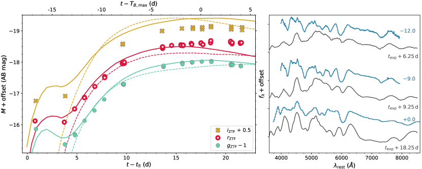
Figure 12: Comparison of SN 2019yvq and our model with a 0.02 $M_{\odot}$ clump of ⁵⁶Ni in the outer ejecta. For the comparison we have adopted a model explosion time $t_{\mathrm{exp}}=t_{\mathrm{fl}}-0.8$ d. Left: photometric comparison between SN 2019yvq and the model. Symbols are the same as Figure 1. The clump model is shown via solid lines, while the best-fit model for the “normal” rise is shown as dashed lines. The clump models have been offset by $-0.1$ mag to account for the blanketing due to the clump (see text). The Ni-clump model provides an adequate match to the flash in the $g_{\mathrm{ZTF}}$- and $r_{\mathrm{ZTF}}$-bands. Right: spectroscopic comparison between SN 2019yvq and the model. Observed spectra of SN 2019yvq are shown in blue, with phases marked relative to $T_{B,\mathrm{max}}$, whereas the model spectra are shown in dark gray, with phases marked relative to the modeled time of explosion. The modeled spectra have been smoothed with a Savitzky-Golay filter (Savitzky & Golay, 1964). While an extended clump of ⁵⁶Ni in the SN ejecta can produce an early optical flash, it leads to strong blanketing in the blue portion of the optical spectra ($\lambda\lesssim 4400$ Å) that is not observed around maximum light in SN 2019yvq.

For SN 2019yvq we follow the procedure in Magee & Maguire (2020) to model the early flash and rise of the SN. As described in the beginning of §6, we generate a “baseline” model that replicates the rise of SN 2019yvq after the first two epochs of ZTF optical detections. Following the generation of this “baseline” model, we add clumps of ⁵⁶Ni to the outer layers of the SN ejecta, and perform full radiative transfer calculations using TURTLS (Magee et al., 2018).

We find that a model with a 0.02 $M_{\rm{\odot}}$ clump of ⁵⁶Ni adequately matches the early optical evolution of SN 2019yvq in the $g_{\mathrm{ZTF}}$ and $r_{\mathrm{ZTF}}$-bands, as shown in Figure 12. The model flux in the $i_{\mathrm{ZTF}}$-band is overestimated, however, meaning the model is redder than what is observed. In Figure 12, the Ni-clump models have been offset by $-0.1$ mag to better match the observations. This offset is necessary as the Ni clump provides some blanketing around maximum light, and the parameter space is too large to simultaneously optimize both the central Ni mass and the clump Ni mass.

While a clump of ⁵⁶Ni can produce an optical bump in the light curve, the same challenges identified in Magee & Maguire (2020) apply to SN 2019yvq. In particular, an extended clump of ⁵⁶Ni dramatically alters the appearance of the SN at maximum light. Figure 12 shows a comparison of the observed spectra with our calculated models. The Ni-clump models feature strong blanketing in the blue-optical region of the spectrum, which is simply not present in the observed spectra of SN 2019yvq. We therefore conclude that Ni clumps cannot explain the early flash seen in SN 2019yvq.

6.3 Double-Detonation Models

WDs that accrete a thin shell of He can explode via a “double detonation” whereby explosive burning in the He shell drives a shock into the C/O core of the WD. This shock can ignite explosive C burning and trigger a detonation that disrupts the entire star (e.g., Nomoto 1982a, b; Woosley & Weaver 1994). Such explosions are even possible in C/O WDs that are well below the Chandrasekhar mass (see Fink et al. 2007, 2010 and references therein).

Recent models of double-detonation explosions presented in Polin et al. (2019a) show that such explosions can replicate several of the peculiar properties of SN 2019yvq, including the early UV/optical flash, a blue to red to blue color transition, the moderately faint optical peak, red colors at maximum, and a lack of IGE in the early spectra.

The appearance of double-detonation SNe is effectively determined by two properties: the mass of the C/O core and the mass of the He shell. The total mass of the system determines the central density of the WD and thus the amount of synthesized ⁵⁶Ni. The ⁵⁶Ni mass directly controls both the peak luminosity and the kinetic energy of the explosion. High mass WDs ($\gtrsim 1.1\,M_{\odot}$) create enough ⁵⁶Ni ($M_{\mathrm{Ni}}\gtrsim 0.5\,M_{\odot}$) to produce large ($\gtrsim 1$4,000 km s^-1) photospheric velocities and reach normal brightness for an SN Ia, while low mass WDs ($\lesssim 0.9\,M_{\odot}$) exhibit lower photospheric velocities ($\lesssim 1$0,000 km s^-1) and produce less ⁵⁶Ni, therefore peaking at fainter luminosities (Polin et al., 2019a). That we see both a high Si II velocity and a low peak luminosity in SN 2019yvq presents a challenge for the Polin et al. (2019a) double-detonation models (see their Figure 11). Furthermore, thick He shells ($M_{\mathrm{He}}\gtrsim 0.05\,M_{\odot}$) produce more pronounced UV/optical flashes shortly after explosion, particularly in conjunction with lower mass WDs, while thin He shells ($M_{\mathrm{He}}\lesssim 0.02\,M_{\odot}$) produce a more extreme color inversion in the days after explosion.

We have attempted to model the evolution of SN 2019yvq as a double-detonation explosion, following the procedure in Polin et al. (2019a). We have specifically focused on matching the photometric evolution (as noted above no models create high-velocity ejecta and underluminous optical peaks), with particular attention to the colors during the early flash and at maximum light. We find that a model with $M_{\mathrm{C/O}}=0.92\,M_{\odot}$ C/O core and a $M_{\mathrm{He}}=0.04\,M_{\odot}$ He shell best match SN 2019yvq, as shown in Figure 13.

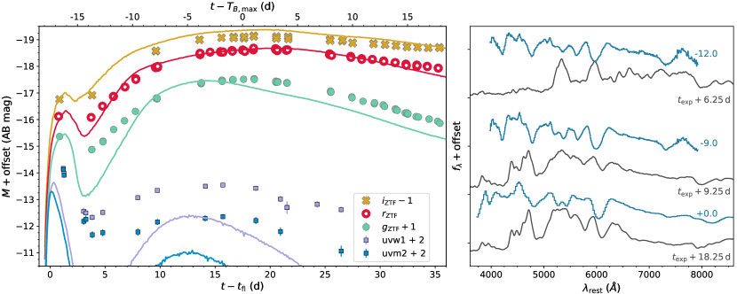
Figure 13: Comparison of SN 2019yvq to a double-detonation model with a C/O core mass $M_{\mathrm{C/O}}=0.92\,M_{\odot}$ and He shell mass $M_{\mathrm{He}}=0.04\,M_{\odot}$ (i.e., $M_{\mathrm{WD}}=0.96\,M_{\odot}$). For the comparison we have adopted a model explosion time $t_{\mathrm{exp}}=t_{\mathrm{fl}}-0.72$ d. Left: photometric comparison between SN 2019yvq and the model. Symbols are the same as Figure 1. The double-detonation model provides a good match to the $r_{\mathrm{ZTF}}$-band evolution, though the flux in the $g_{\mathrm{ZTF}}$- and $i_{\mathrm{ZTF}}$-bands is under- and overpredicted, respectively. The UV emission is also underestimated by the double-detonation model. Right: spectroscopic comparison between SN 2019yvq and the model. Observed spectra of SN 2019yvq are shown in blue, with phases marked relative to $T_{B,\mathrm{max}}$, whereas the model spectra are shown in dark gray, with phases marked relative to the modeled time of explosion. The modeled spectra have been smoothed with a Savitzky-Golay filter (Savitzky & Golay, 1964). The photospheric velocity in the double-detonation model is lower than what is observed in SN 2019yvq, and the models feature more absorption and blanketing in the blue portion of the optical than what is observed.

While this model adequately matches the evolution of SN 2019yvq in the $r_{\mathrm{ZTF}}$ filter, the predictions in the $g_{\mathrm{ZTF}}$- and $i_{\mathrm{ZTF}}$-bands do not match what is observed. We show for the first time that there is an expected UV flash associated with these double-detonation models, however, our best-fit model underestimates the flux that was observed in the UV.

Synthesized spectra from our double-detonation model exhibit features that are not seen in SN 2019yvq. The model spectra are dominated by Si II absorption, and show high-velocity absorption due to O I and Ca II, similar to SN 2019yvq. For our best-fit model, however, the Si II velocities are too slow, the Si II $\lambda$5972 absorption is too strong, and the S II absorption is too weak. Nuclear burning in the He shell creates heavy elements in the outermost ejecta of double-detonation explosions, leading to deep Ti II troughs and other blanketing in the blue-optical portion of the spectrum. Our model exhibits a strong Ti II absorption trough blueward of $\sim$4400 Å (see the $t_{\mathrm{exp}}+9.25$ d spectrum in Figure 13). As was the case for models with extended clumps of ⁵⁶Ni, the lack of such absorption in SN 2019yvq poses a challenge for the double-detonation model.

With observations that probe a previously unexplored phase in the evolution of such explosions, SN 2019yvq provides an opportunity to determine where the double-detonation models must improve. It is possible that such improvements could lead to better agreement with SN 2019yvq. For instance, the nuclear reaction networks and 1D models in Polin et al. (2019a) always burn the He shells to nuclear statistical equilibrium. It is not unreasonable to think that 2D or 3D models, with a more sophisticated nuclear reaction network, would create more IMEs and less IGEs in the He shell, and that the ratio of the two created in the shell could be highly dependent upon the line of sight. For example, Townsley et al. (2019) modeled the explosion of a $M_{\mathrm{C/O}}=1.0\,M_{\odot}$ C/O core with a $M_{\mathrm{He}}=0.02\,M_{\odot}$ He shell and found a higher ratio of IME to IGE than the analogous 1D model presented in Polin et al. (2019a, though see also , which presents a 3D double-detonation explosion with nuclear yields that are only mildly different from 1D models). This could explain the lack of IGEs and strong Si II absorption seen in the early spectra, while less IGEs in the outer layers would also reduce some of the line blanketing seen around maximum light. This would lead to less reprocessing of blue photons, perhaps creating better agreement between the models and photometry, particularly in the $g_{\mathrm{ZTF}}$-band. The velocity discrepancy could also potentially be explained as a line-of-sight effect. If the ignition of the WD occurred off center, then the ejecta aligned with the site of the initial He ignition may receive a boost in velocity (e.g., Kromer et al., 2010). The discrepancies in the UV are less worrisome. While we show a qualitative UV flash, the magnitude of this flash will be highly sensitive to the precise temperature and composition in the very outermost ejecta, and thus any of the changes discussed above could easily boost the model flux in the UV.

6.4 Violent Mergers and Circumstellar Interaction

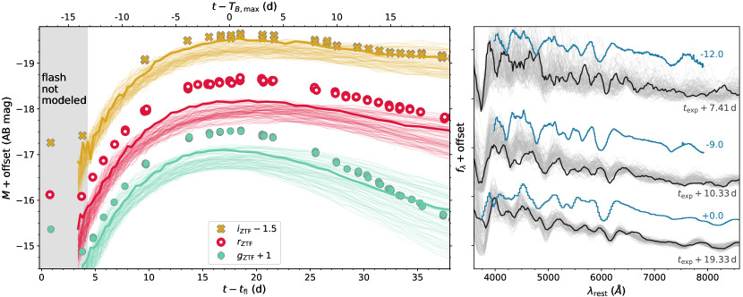
Figure 14: Comparison of SN 2019yvq to the low-metallicity ($Z=0.01Z_{\odot}$) violent merger model of a 0.9 and 0.76 $M_{\odot}$ WD from Kromer et al. (2016). This model provides a good match to iPTF 14atg, and therefore significantly underestimates the brightness of SN 2019yvq. For the comparison we have adopted a model explosion time of $t_{\mathrm{exp}}=t_{\mathrm{fl}}-1.92$ d. Thin lines represent one of 100 sightlines, while the bold lines represent a single sightline for illustrative purposes. Left: photometric comparison between SN 2019yvq and the model. Symbols are the same as those in Figure 1. The shaded area shows the UV/optical flash from SN 2019yvq, which was not modeled by Kromer et al. (2016). Despite the underestimated optical flux, the qualitative behavior of the violent merger model, including red $g_{\mathrm{ZTF}}$$-$$r_{\mathrm{ZTF}}$ colors at peak and a lack of secondary maximum in the $i_{\mathrm{ZTF}}$-band do match SN 2019yvq. Right: Spectroscopic comparison between SN 2019yvq and the violent merger model. Observed spectra of SN 2019yvq are shown in blue, with phases marked relative to $T_{B,\mathrm{max}}$, whereas the model spectra are shown as thin gray lines. The thick black line highlights a specific viewing angle. The modeled spectra have been smoothed with a Savitzky-Golay filter (Savitzky & Golay, 1964). The photospheric velocity in the violent merger model features lower velocities than SN 2019yvq, while the strength of the the IME absorption is weaker in the models than what is observed.

Piro & Morozova (2016) show that circumstellar material in the vicinity of a WD at the time of explosion can give rise to an early flash or bump in the SN Ia light curve. Using a 1D toy model, with an assumed circumstellar density profile $\propto r^{-3}$ and gray opacities, Piro & Morozova (2016) found that the peak of the early emission is roughly proportional to the extent of the circumstellar material, while the duration of the flash is proportional to the square root of the circumstellar mass. While the brightest model from Piro & Morozova (2016) has a flash brightness that peaks at $M_{V}\approx-15$ mag, circumstellar material that extends beyond $\sim$10¹² cm could give rise to a flash that peaks at $M_{g}\lesssim-16.4$ mag, as is observed in SN 2019yvq.

There are few proposed WD explosion models that produce dense circumstellar material in the vicinity of the WD at the time of explosion. A notable exception is the violent merger, so called because the thermonuclear explosion happens while the merger is still ongoing, of two C/O WDs (Pakmor et al., 2010, 2011, 2012). DD mergers should produce a wide variety of circumstellar configurations, depending on the initial parameters of the inspiralling binary, which would, in turn, produce different signals shortly after explosion (e.g., Raskin & Kasen 2013; Levanon & Soker 2019).

Given the vast parameter space populated by different circumstellar configurations, we are going to proceed under the (potentially poor) assumption that such interaction could reproduce the UV/optical flash seen in SN 2019yvq. Following this assumption, a relevant question is – can violent mergers reproduce the properties of SN 2019yvq in the days before and weeks after $T_{B,\mathrm{max}}$?

In Kromer et al. (2016), the violent merger of two C/O WDs with masses of 0.9 and 0.76 $M_{\odot}$ produced a similar rise and maximum-light properties to iPTF 14atg, the other SN Ia with an observed early UV flash. A comparison of SN 2019yvq to the low-metallicity model from Kromer et al. (2016), which provides a good match to iPTF 14atg, is shown in Figure 14. We show that model here to illustrate the qualitative behavior of such a merger; it is not meant to provide an optimal match to SN 2019yvq. The Kromer et al. model was not designed to fit the early UV flash in iPTF 14atg.

The photometric evolution of this violent merger model qualitatively matches SN 2019yvq: (i) a moderately faint peak in the optical ($-17.6\,\mathrm{mag}\gtrsim M_{g}\gtrsim-18.2$ mag, depending on the viewing angle), (ii) red $g-r$ colors at peak, and (iii) a lack of a secondary maximum in the $i$-band. Furthermore, the spectra lack significant IGE absorption in the days after explosion (right panel of Figure 14), as is observed in SN 2019yvq. Interestingly, the violent merger model does show a decrease in the relative strength of the Si II $\lambda$5972 absorption with time, similar to SN 2019yvq and unlike the other models considered here. A critical difference between SN 2019yvq and violent merger models, is that the merger models tend to produce relatively low expansion velocities (e.g., Pakmor et al. 2010; Kromer et al. 2013, 2016). Indeed, this is one of the stark differences between SN 2019yvq and iPTF 14atg, as iPTF 14atg had a Si II $\lambda$6355 absorption velocity of $\sim$7500 km s^-1 at peak, or roughly half that observed in SN 2019yvq. It is also clear from Figure 14 that the violent merger model from Kromer et al. (2016) exhibits weaker IME absorption than what is seen in SN 2019yvq.

It is clear that additional modeling, likely of a different WD binary configuration, is needed to better match SN 2019yvq. For example, it is known that a higher mass primary WD can produce more ⁵⁶Ni, and hence a brighter optical peak (e.g., Pakmor et al., 2012), which would be more in line with SN 2019yvq. If, at the same time, the mass of the secondary were slightly decreased, then the kinetic energy of the ejecta would increase, perhaps bringing the model velocity of Si II and other IMEs in line with SN 2019yvq. It would also be beneficial to track the unbound material following the DD merger, to see if the collision between this material and the SN ejecta can replicate the early UV/optical flash seen in SN 2019yvq. If this feature can readily be recreated, it is possible that a violent merger is responsible for SN 2019yvq.

7 Discussion

Table 6: Summary of Observational Properties of SN 2019yvq

	Does the Model Replicate this Property?
	UV	Low Peak	Intermediate/Fast	Red Colors	Lack of IGE	$\mathcal{R}($Si II$)$	High Si II
Model	Flash	Luminosity	Decline	at All Epochs	in Early Spectra	Evolution	Velocities
Companion interaction	✓	?	?	?	?	?	?
56Ni clumps	✓	?	?	✓	✗	?	?
He shell double detonation	✓	✓	✓	✓	✗	✗	✗
Violent merger	?	✓	✓	✓	✓	✓	✗

Note. — If a model replicates a specific property we show a ✓, whereas properties that are not matched are signified with an ✗. Ambiguous cases are shown as ?. An important distinction for the companion-interaction and ⁵⁶Ni-clump models is that they are empirical, whereas the double-detonation and violent merger models are based on a specific realization of an exploding WD. Given that the companion-interaction and ⁵⁶Ni-clump models do not model the explosion itself, we label all properties that are not generic to the class as ?. While the double-detonation and ⁵⁶Ni-clump models produce a UV flash, it is unclear whether or not they can match the magnitude of the observed flash in SN 2019yvq. The violent merger model does not track circumstellar material, and additional simulations are needed to understand whether interaction between the ejecta and unbound material could reproduce the UV flash (see text). In addition to showing evidence for IGE absorption in the early spectra, the double-detonation and ⁵⁶Ni-clump models show strong IGE absorption and line blanketing around maximum light that is not observed in SN 2019yvq.

We have presented observations of the spectacular SN 2019yvq, the second observed SN Ia to exhibit a clear UV/optical flash in its early evolution. Despite this dazzling, declarative display announcing SN 2019yvq as a unique event among the thousands of SNe Ia that have previously been cataloged, we find that SN 2019yvq would be considered unusual even if the early flash had been missed.

The photometric evolution of SN 2019yvq resembles that of the intermediate 86G-like subclass of SNe Ia. With a moderately faint peak in the optical ($M_{g}\approx-18.5$ mag), relatively fast decline [$\Delta m_{15}(g)=1.3$ mag], and lack of a secondary maximum in the $i_{\mathrm{ZTF}}$ filter, SN 2019yvq is clearly distinguished photometrically from normal SNe Ia. These photometric properties typically correspond to Branch Cool SNe, yet the spectroscopic evolution of SN 2019yvq does not match such events. SN 2019yvq is a Branch Broad Line SN, with relatively weak Si II $\lambda$5972 absorption and large Si II velocities. Furthermore, our TARDIS spectral models show little to no IGE present in the outer layers of the SN ejecta, which further distinguishes SN 2019yvq, even relative to other Branch Broad Line SNe. The fact that SN 2019yvq exhibits high-velocity Si II $\lambda$6355 absorption and an underluminous peak sets it apart from other SNe Ia.

SN 2019yvq is one of a growing group of SNe Ia with photometric properties that may or may not deviate from the standard width-luminosity relationship for normal SNe Ia (e.g., Phillips, 1993; Phillips et al., 1999), but whose spectral evolution is incongruous with their photometric properties. While these SNe all differ in detail, many can be linked via the presence of 91bg-like spectroscopic features, such as the Ti II “trough” at $\sim$4200 Å (Filippenko et al., 1992; Leibundgut et al., 1993), despite relatively broad light curves that are more consistent with normal or intermediate SNe Ia (examples include: SN 2006bt, Foley et al. 2010; PTF 10ops, Maguire et al. 2011; SN 2006ot, Stritzinger et al. 2011; SN 2010lp, Kromer et al. 2013; SN 2002es, Ganeshalingam et al. 2012; and iPTF 14atg, Cao et al. 2015).

Benetti et al. (2005) showed that photometric and spectroscopic properties of SNe Ia are closely linked by connecting normal and subluminous 91bg-like SNe Ia in a tight sequence in the $\mathcal{R}($Si II$)$–$\Delta m_{15}(B)$ plane. As first pointed out in Foley et al. (2010) and later confirmed by Maguire et al. (2011) and Ganeshalingam et al. (2012), the peculiar SNe mentioned above starkly standout from the simple sequence found in Benetti et al. (2005) as the peculiar SNe all have $\mathcal{R}($Si II$)$ values that are much higher than expected given their decline rate as parameterized by $\Delta m_{15}(B)$. SN 2019yvq also stands out in this plane, though in the opposite sense, the low $\mathcal{R}($Si II$)$ at maximum light (§5.2) suggests a slow decline, which is not observed (§4.4). Whether these events all feature a common origin remains to be seen, though it is interesting that the two events with observed early UV flashes, iPTF 14atg and SN 2019yvq, are both peculiar and possibly connected as outliers in the $\mathcal{R}($Si II$)$–$\Delta m_{15}(B)$ plane.

We have found that building a consistent physical model to explain all of the observed properties of SN 2019yvq is challenging. Most models either replicate the early flash but fail to reproduce the observed behavior around maximum light, or vice versa.

We have examined four models in detail to try to explain the dramatic early UV/optical peak in SN 2019yvq, including the collision of the SN ejecta with a nondegenerate companion (e.g., Kasen 2010), extended clumps of ⁵⁶Ni in the outer layers of the SN ejecta (e.g., Magee & Maguire, 2020), the double-detonation explosion of a sub-Chandrasekhar mass WD (e.g., Polin et al., 2019a), and the violent merger of two sub-Chandrasekhar mass WDs (e.g., Kromer et al., 2016). Table 6 summarizes the key observational properties of SN 2019yvq listed in §6 and whether or not these four models can explain the different aspects of SN 2019yvq.

The SN ejecta-companion models, which can easily replicate the early UV flash from SN 2019yvq, simultaneously overpredict the optical flux at similar epochs. Models with extended clumps of ⁵⁶Ni produce significant blanketing in the blue-optical region of the spectrum. While the double-detonation model produces an early flash and $r_{\mathrm{ZTF}}$ evolution that provides a good match to SN 2019yvq, it too produces blanketing that is too strong relative to the blue-optical spectra and features absorption velocities that are much lower than what is observed. The specific WD merger model from Kromer et al. (2016) that we compare to SN 2019yvq does a poor job of replicating the observations. Many of the qualitative features match, however, so it is not unreasonable to think that with some tuning (e.g., higher mass WDs) the merger model could better reflect what is observed in SN 2019yvq.

While we have focused on explaining the spectacular UV flash, we were also unable to identify any models that match the maximum-light properties of SN 2019yvq. One possibility to explain the low ⁵⁶Ni yield and large Si II velocities would be to terminate a lot of the nuclear burning at IMEs, which, in turn, would result in a relatively low fraction of IGE. Such a scenario may be possible at low central densities, which would keep the IGE fraction in the ejecta low, if enough material burns (in order to release a sufficient amount of energy to accelerate the ejecta to high velocities). Further work is needed, however, to know whether such a scenario could be produced by realistic binaries in nature.

Nebular spectra of SN 2019yvq will play a crucial role in disambiguating between these various scenarios. If the ejecta have collided with a nondegenerate companion, then they will have stripped some surface material from the companion, which will be revealed via narrow Balmer lines in the nebular phase (e.g., Wheeler et al., 1975). Alternatively, Polin et al. (2019b) recently showed that low mass ($M_{\mathrm{WD}}\lesssim 1.0\,M_{\odot}$) double-detonation explosions do not create a significant amount of IGEs in their core. This relative lack of IGEs means that [Ca II] provides the best pathway for the ejecta to cool, and as a result strong [Ca II] $\lambda\lambda$7291, 7324 emission is expected in the nebular phase. Finally, violent mergers are expected to exhibit narrow [O I] $\lambda\lambda$6300, 6364 emission in their nebular spectra, as unburned O from the disrupted WD is present at low velocities in the central ejecta (Taubenberger et al., 2013; Kromer et al., 2016). Each of these predictions are unique to the scenarios discussed here.

The critical challenge moving forward in understanding SN 2019yvq-like events is the rapid acquisition of UV observations shortly after explosion. ZTF, and other similar surveys (ATLAS, ASAS-SN; Tonry 2011; Holoien et al. 2017), have demonstrated the ability to routinely find extremely young SNe Ia. Following this the challenge is to (i) recognize these events as likely SNe Ia at the epoch of discovery (i.e., without a significant delay to obtain a spectroscopic classification) and (ii) promptly obtain Swift photometry. While the presence of an early UV flash may be intrinsically rare, in the past $\sim$7 yr it has only been observed twice, it seems more likely that the above process (discovery, classification, Swift ToO) is highly incomplete. Furthermore, if a typical UV flash is either less luminous or of a shorter duration than what was observed in iPTF 14atg and SN 2019yvq, then the chain of events leading to Swift observations may be insufficient to regularly capture such a signal. It would be far more efficient to search for such flashes directly using a wide-field UV telescope (e.g., Sagiv et al., 2014). Only after extremely early UV observations become as routine as the discoveries themselves will we be able to statistically constrain the models discussed herein, and, as a result, answer fundamental questions about the nature of SN Ia progenitors.

References

- Abolfathi et al. (2018) Abolfathi, B., Aguado, D. S., Aguilar, G., et al. 2018, ApJS, 235, 42
- Almgren et al. (2010) Almgren, A. S., Beckner, V. E., Bell, J. B., et al. 2010, ApJ, 715, 1221
- Arnett (1982) Arnett, W. D. 1982, ApJ, 253, 785
- Astropy Collaboration et al. (2013) Astropy Collaboration, Robitaille, T. P., Tollerud, E. J., et al. 2013, A&A, 558, A33
- Barbary et al. (2016) Barbary, K., Barclay, T., Biswas, R., et al. 2016, SNCosmo: Python library for supernova cosmology
- Barnsley et al. (2012) Barnsley, R. M., Smith, R. J., & Steele, I. A. 2012, AN, 333, 101
- Bellm & Sesar (2016) Bellm, E. C., & Sesar, B. 2016, pyraf-dbsp: Reduction pipeline for the Palomar Double Beam Spectrograph
- Bellm et al. (2019a) Bellm, E. C., Kulkarni, S. R., Graham, M. J., et al. 2019a, PASP, 131, 018002
- Bellm et al. (2019b) Bellm, E. C., Kulkarni, S. R., Barlow, T., et al. 2019b, PASP, 131, 068003
- Benetti et al. (2004) Benetti, S., Meikle, P., Stehle, M., et al. 2004, MNRAS, 348, 261
- Benetti et al. (2005) Benetti, S., Cappellaro, E., Mazzali, P. A., et al. 2005, ApJ, 623, 1011
- Bianco et al. (2011) Bianco, F. B., Howell, D. A., Sullivan, M., et al. 2011, ApJ, 741, 20
- Blagorodnova et al. (2018) Blagorodnova, N., Neill, J. D., Walters, R., et al. 2018, PASP, 130, 035003
- Blondin et al. (2012) Blondin, S., Matheson, T., Kirshner, R. P., et al. 2012, AJ, 143, 126
- Bloom et al. (2012) Bloom, J. S., Kasen, D., Shen, K. J., et al. 2012, ApJ, 744, L17
- Branch et al. (2006) Branch, D., Dang, L. C., Hall, N., et al. 2006, PASP, 118, 560
- Breeveld et al. (2011) Breeveld, A. A., Landsman, W., Holland, S. T., et al. 2011, American Institute of Physics Conference Series, 1358, 373
- Brown et al. (2014) Brown, P. J., Breeveld, A. A., Holland, S., et al. 2014, Ap&SS, 354, 89
- Brown et al. (2012) Brown, P. J., Dawson, K. S., Harris, D. W., et al. 2012, ApJ, 749, 18
- Brown et al. (2017) Brown, P. J., Landez, N. J., Milne, P. A., & Stritzinger, M. D. 2017, ApJ, 836, 232
- Brown et al. (2019) Brown, P. J., Hosseinzadeh, G., Jha, S. W., et al. 2019, ApJ, 877, 152
- Bulla et al. (2020) Bulla, M., Miller, A. A., Yao, Y., et al. 2020, arXiv, arXiv:2001.00587
- Burns et al. (2011) Burns, C. R., Stritzinger, M., Phillips, M. M., et al. 2011, AJ, 141, 19
- Burns et al. (2014) —. 2014, ApJ, 789, 32
- Burrows et al. (2005) Burrows, D. N., Hill, J. E., Nousek, J. A., et al. 2005, Space Sci. Rev., 120, 165
- Cao et al. (2015) Cao, Y., Kulkarni, S. R., Howell, D. A., et al. 2015, Nature, 521, 328
- Carrick et al. (2015) Carrick, J., Turnbull, S. J., Lavaux, G., & Hudson, M. J. 2015, MNRAS, 450, 317
- Contardo et al. (2000) Contardo, G., Leibundgut, B., & Vacca, W. D. 2000, A&A, 359, 876
- Cristiani et al. (1992) Cristiani, S., Cappellaro, E., Turatto, M., et al. 1992, A&A, 259, 63
- De et al. (2019) De, K., Kasliwal, M. M., Polin, A., et al. 2019, ApJ, 873, L18
- De et al. (2020) De, K., Kasliwal, M. M., Tzanidakis, A., et al. 2020, arXiv, arXiv:2004.09029
- de Vaucouleurs et al. (1991) de Vaucouleurs, G., de Vaucouleurs, A., Corwin, Herold G., J., et al. 1991, Third Reference Catalogue of Bright Galaxies
- Dekany et al. (2020) Dekany, R., Smith, R. M., Riddle, R., et al. 2020, PASP, 132, 038001
- Dessart et al. (2014) Dessart, L., Blondin, S., Hillier, D. J., & Khokhlov, A. 2014, MNRAS, 441, 532
- Dhawan et al. (2018) Dhawan, S., Bulla, M., Goobar, A., et al. 2018, MNRAS, 480, 1445
- Dimitriadis et al. (2019) Dimitriadis, G., Foley, R. J., Rest, A., et al. 2019, ApJ, 870, L1
- Evans et al. (2007) Evans, P. A., Beardmore, A. P., Page, K. L., et al. 2007, A&A, 469, 379
- Evans et al. (2009) —. 2009, MNRAS, 397, 1177
- Fabricant et al. (2019) Fabricant, D., Fata, R., Epps, H., et al. 2019, PASP, 131, 075004
- Filippenko et al. (1992) Filippenko, A. V., Richmond, M. W., Branch, D., et al. 1992, AJ, 104, 1543
- Fink et al. (2007) Fink, M., Hillebrandt, W., & Röpke, F. K. 2007, A&A, 476, 1133
- Fink et al. (2010) Fink, M., Röpke, F. K., Hillebrandt, W., et al. 2010, A&A, 514, A53
- Fink et al. (2014) Fink, M., Kromer, M., Seitenzahl, I. R., et al. 2014, MNRAS, 438, 1762
- Folatelli et al. (2010) Folatelli, G., Phillips, M. M., Burns, C. R., et al. 2010, AJ, 139, 120
- Foley et al. (2010) Foley, R. J., Narayan, G., Challis, P. J., et al. 2010, ApJ, 708, 1748
- Foreman-Mackey (2016) Foreman-Mackey, D. 2016, JOSS, 24
- Foreman-Mackey et al. (2013) Foreman-Mackey, D., Hogg, D. W., Lang, D., & Goodman, J. 2013, PASP, 125, 306
- Fremling et al. (2020) Fremling, C., Miller, A. A., Sharma, Y., et al. 2020, ApJ, 895, 32
- Ganeshalingam et al. (2011) Ganeshalingam, M., Li, W., & Filippenko, A. V. 2011, MNRAS, 416, 2607
- Ganeshalingam et al. (2012) Ganeshalingam, M., Li, W., Filippenko, A. V., et al. 2012, ApJ, 751, 142
- Gehrels et al. (2004) Gehrels, N., Chincarini, G., Giommi, P., et al. 2004, ApJ, 611, 1005
- Goobar et al. (2015) Goobar, A., Kromer, M., Siverd, R., et al. 2015, ApJ, 799, 106
- Goodman & Weare (2010) Goodman, J., & Weare, J. 2010, CAMCS, 5, 65
- Graham et al. (2019) Graham, M. J., Kulkarni, S. R., Bellm, E. C., et al. 2019, PASP, 131, 078001
- Gronow et al. (2020) Gronow, S., Collins, C., Ohlmann, S. T., et al. 2020, A&A, 635, A169
- Guy et al. (2007) Guy, J., Astier, P., Baumont, S., et al. 2007, A&A, 466, 11
- Hachinger et al. (2008) Hachinger, S., Mazzali, P. A., Tanaka, M., et al. 2008, MNRAS, 389, 1087
- Hachinger et al. (2013) Hachinger, S., Mazzali, P. A., Sullivan, M., et al. 2013, MNRAS, 429, 2228
- Hayden et al. (2010) Hayden, B. T., Garnavich, P. M., Kessler, R., et al. 2010, ApJ, 712, 350
- HI4PI Collaboration et al. (2016) HI4PI Collaboration, Ben Bekhti, N., Flöer, L., et al. 2016, A&A, 594, A116
- Hillebrandt et al. (2013) Hillebrandt, W., Kromer, M., Röpke, F. K., & Ruiter, A. J. 2013, Frontiers of Physics, 8, 116
- Holoien et al. (2017) Holoien, T. W. S., Stanek, K. Z., Kochanek, C. S., et al. 2017, MNRAS, 464, 2672
- Hosseinzadeh et al. (2017) Hosseinzadeh, G., Sand, D. J., Valenti, S., et al. 2017, ApJ, 845, L11
- Howell et al. (2009) Howell, D. A., Sullivan, M., Brown, E. F., et al. 2009, ApJ, 691, 661
- Hunter (2007) Hunter, J. D. 2007, Computing In Science & Engineering, 9, 90
- Itagaki (2019) Itagaki, K. 2019, Transient Name Server Discovery Report, 2019-2720, 1
- Jeffery (1999) Jeffery, D. J. 1999, arXiv, astro
- Jiang et al. (2018) Jiang, J.-a., Doi, M., Maeda, K., & Shigeyama, T. 2018, ApJ, 865, 149
- Jiang et al. (2017) Jiang, J.-A., Doi, M., Maeda, K., et al. 2017, Nature, 550, 80
- Kasen (2010) Kasen, D. 2010, ApJ, 708, 1025
- Kasen et al. (2006) Kasen, D., Thomas, R. C., & Nugent, P. 2006, ApJ, 651, 366
- Kawabata (2020) Kawabata, M. 2020, Transient Name Server Classification Report, 2020-24, 1
- Kerzendorf & Sim (2014) Kerzendorf, W. E., & Sim, S. A. 2014, MNRAS, 440, 387
- Khokhlov (1991) Khokhlov, A. M. 1991, A&A, 245, 114
- Krisciunas et al. (2017) Krisciunas, K., Contreras, C., Burns, C. R., et al. 2017, AJ, 154, 211
- Kromer et al. (2017) Kromer, M., Ohlmann, S., & Röpke, F. K. 2017, Mem. Soc. Astron. Italiana, 88, 312
- Kromer et al. (2010) Kromer, M., Sim, S. A., Fink, M., et al. 2010, ApJ, 719, 1067
- Kromer et al. (2013) Kromer, M., Pakmor, R., Taubenberger, S., et al. 2013, ApJ, 778, L18
- Kromer et al. (2016) Kromer, M., Fremling, C., Pakmor, R., et al. 2016, MNRAS, 459, 4428
- Leibundgut et al. (1993) Leibundgut, B., Kirshner, R. P., Phillips, M. M., et al. 1993, AJ, 105, 301
- Levanon & Soker (2017) Levanon, N., & Soker, N. 2017, MNRAS, 470, 2510
- Levanon & Soker (2019) —. 2019, ApJ, 872, L7
- Maeda et al. (2018) Maeda, K., Jiang, J.-a., Shigeyama, T., & Doi, M. 2018, ApJ, 861, 78
- Magee & Maguire (2020) Magee, M. R., & Maguire, K. 2020, arXiv, arXiv:2007.02101
- Magee et al. (2020) Magee, M. R., Maguire, K., Kotak, R., et al. 2020, A&A, 634, A37
- Magee et al. (2018) Magee, M. R., Sim, S. A., Kotak, R., & Kerzendorf, W. E. 2018, A&A, 614, A115
- Maguire et al. (2011) Maguire, K., Sullivan, M., Thomas, R. C., et al. 2011, MNRAS, 418, 747
- Maguire et al. (2014) Maguire, K., Sullivan, M., Pan, Y. C., et al. 2014, MNRAS, 444, 3258
- Mahabal et al. (2019) Mahabal, A., Rebbapragada, U., Walters, R., et al. 2019, PASP, 131, 038002
- Maoz et al. (2014) Maoz, D., Mannucci, F., & Nelemans, G. 2014, ARA&A, 52, 107
- Marion et al. (2016) Marion, G. H., Brown, P. J., Vinkó, J., et al. 2016, ApJ, 820, 92
- Masci et al. (2019) Masci, F. J., Laher, R. R., Rusholme, B., et al. 2019, PASP, 131, 018003
- Mazzali et al. (2014) Mazzali, P. A., Sullivan, M., Hachinger, S., et al. 2014, MNRAS, 439, 1959
- McKinney (2010) McKinney, W. 2010, 51
- Miller et al. (2018) Miller, A. A., Cao, Y., Piro, A. L., et al. 2018, ApJ, 852, 100
- Miller et al. (2020) Miller, A. A., Yao, Y., Bulla, M., et al. 2020, arXiv, arXiv:2001.00598
- Mould et al. (2000) Mould, J. R., Huchra, J. P., Freedman, W. L., et al. 2000, ApJ, 529, 786
- Nadyozhin (1994) Nadyozhin, D. K. 1994, ApJS, 92, 527
- NASA High Energy Astrophysics Science Archive Research Center (2014) (HEASARC) NASA High Energy Astrophysics Science Archive Research Center (HEASARC). 2014, HEAsoft: Unified Release of FTOOLS and XANADU
- Noebauer et al. (2017) Noebauer, U. M., Kromer, M., Taubenberger, S., et al. 2017, MNRAS, 472, 2787
- Nomoto (1982a) Nomoto, K. 1982a, ApJ, 253, 798
- Nomoto (1982b) —. 1982b, ApJ, 257, 780
- Nugent et al. (1995) Nugent, P., Phillips, M., Baron, E., et al. 1995, ApJ, 455, L147
- Nugent et al. (2011) Nugent, P. E., Sullivan, M., Cenko, S. B., et al. 2011, Nature, 480, 344
- Oke & Gunn (1982) Oke, J. B., & Gunn, J. E. 1982, PASP, 94, 586
- Oke et al. (1995) Oke, J. B., Cohen, J. G., Carr, M., et al. 1995, PASP, 107, 375
- Olling et al. (2015) Olling, R. P., Mushotzky, R., Shaya, E. J., et al. 2015, Nature, 521, 332
- Pakmor et al. (2011) Pakmor, R., Hachinger, S., Röpke, F. K., & Hillebrand t, W. 2011, A&A, 528, A117
- Pakmor et al. (2010) Pakmor, R., Kromer, M., Röpke, F. K., et al. 2010, Nature, 463, 61
- Pakmor et al. (2012) Pakmor, R., Kromer, M., Taubenberger, S., et al. 2012, ApJ, 747, L10
- Pastorello et al. (2007) Pastorello, A., Mazzali, P. A., Pignata, G., et al. 2007, MNRAS, 377, 1531
- Patterson et al. (2019) Patterson, M. T., Bellm, E. C., Rusholme, B., et al. 2019, PASP, 131, 018001
- Pedregosa et al. (2011) Pedregosa, F., Varoquaux, G., Gramfort, A., et al. 2011, Journal of Machine Learning Research, 12, 2825
- Pereira et al. (2013) Pereira, R., Thomas, R. C., Aldering, G., et al. 2013, A&A, 554, A27
- Perley (2019) Perley, D. A. 2019, PASP, 131, 084503
- Phillips (1993) Phillips, M. M. 1993, ApJ, 413, L105
- Phillips et al. (1999) Phillips, M. M., Lira, P., Suntzeff, N. B., et al. 1999, AJ, 118, 1766
- Phillips et al. (1987) Phillips, M. M., Phillips, A. C., Heathcote, S. R., et al. 1987, PASP, 99, 592
- Phillips et al. (2013) Phillips, M. M., Simon, J. D., Morrell, N., et al. 2013, ApJ, 779, 38
- Piascik et al. (2014) Piascik, A. S., Steele, I. A., Bates, S. D., et al. 2014, Society of Photo-Optical Instrumentation Engineers (SPIE) Conference Series, Vol. 9147, SPRAT: Spectrograph for the Rapid Acquisition of Transients, 91478H
- Piro et al. (2010) Piro, A. L., Chang, P., & Weinberg, N. N. 2010, ApJ, 708, 598
- Piro & Morozova (2016) Piro, A. L., & Morozova, V. S. 2016, ApJ, 826, 96
- Polin et al. (2019a) Polin, A., Nugent, P., & Kasen, D. 2019a, ApJ, 873, 84
- Polin et al. (2019b) —. 2019b, arXiv, arXiv:1910.12434
- Poznanski et al. (2012) Poznanski, D., Prochaska, J. X., & Bloom, J. S. 2012, MNRAS, 426, 1465
- Rabinak & Waxman (2011) Rabinak, I., & Waxman, E. 2011, ApJ, 728, 63
- Raskin & Kasen (2013) Raskin, C., & Kasen, D. 2013, ApJ, 772, 1
- Rasmussen & Williams (2006) Rasmussen, C. E., & Williams, C. K. I. 2006, Gaussian Processes for Machine Learning
- Riess et al. (1998) Riess, A. G., Nugent, P., Filippenko, A. V., et al. 1998, ApJ, 504, 935
- Rigault et al. (2019) Rigault, M., Neill, J. D., Blagorodnova, N., et al. 2019, A&A, 627, A115
- Roming et al. (2005) Roming, P. W. A., Kennedy, T. E., Mason, K. O., et al. 2005, Space Science Reviews, 120, 95
- Röpke & Sim (2018) Röpke, F. K., & Sim, S. A. 2018, Space Sci. Rev., 214, 72
- Röpke et al. (2012) Röpke, F. K., Kromer, M., Seitenzahl, I. R., et al. 2012, ApJ, 750, L19
- Sagiv et al. (2014) Sagiv, I., Gal-Yam, A., Ofek, E. O., et al. 2014, AJ, 147, 79
- Savitzky & Golay (1964) Savitzky, A., & Golay, M. J. E. 1964, Analytical Chemistry, 36, 1627
- Scalzo et al. (2014a) Scalzo, R., Aldering, G., Antilogus, P., et al. 2014a, MNRAS, 440, 1498
- Scalzo et al. (2014b) Scalzo, R. A., Ruiter, A. J., & Sim, S. A. 2014b, MNRAS, 445, 2535
- Schlafly & Finkbeiner (2011) Schlafly, E. F., & Finkbeiner, D. P. 2011, ApJ, 737, 103
- Schlegel et al. (1998) Schlegel, D. J., Finkbeiner, D. P., & Davis, M. 1998, ApJ, 500, 525
- Seitenzahl et al. (2013) Seitenzahl, I. R., Ciaraldi-Schoolmann, F., Röpke, F. K., et al. 2013, MNRAS, 429, 1156
- Shappee et al. (2018) Shappee, B. J., Piro, A. L., Stanek, K. Z., et al. 2018, ApJ, 855, 6
- Shappee et al. (2019) Shappee, B. J., Holoien, T. W. S., Drout, M. R., et al. 2019, ApJ, 870, 13
- Shen & Bildsten (2014) Shen, K. J., & Bildsten, L. 2014, ApJ, 785, 61
- Silverman et al. (2011) Silverman, J. M., Ganeshalingam, M., Li, W., et al. 2011, MNRAS, 410, 585
- Sim et al. (2013) Sim, S. A., Seitenzahl, I. R., Kromer, M., et al. 2013, MNRAS, 436, 333
- Steele et al. (2004) Steele, I. A., Smith, R. J., Rees, P. C., et al. 2004, Society of Photo-Optical Instrumentation Engineers (SPIE) Conference Series, Vol. 5489, The Liverpool Telescope: performance and first results, ed. J. Oschmann, Jacobus M., 679
- Stehle et al. (2005) Stehle, M., Mazzali, P. A., Benetti, S., & Hillebrand t, W. 2005, MNRAS, 360, 1231
- Stritzinger et al. (2006) Stritzinger, M., Leibundgut, B., Walch, S., & Contardo, G. 2006, A&A, 450, 241
- Stritzinger et al. (2011) Stritzinger, M. D., Phillips, M. M., Boldt, L. N., et al. 2011, AJ, 142, 156
- Suntzeff (1996) Suntzeff, N. B. 1996, 41
- Taubenberger (2017) Taubenberger, S. 2017, The Extremes of Thermonuclear Supernovae, 317
- Taubenberger et al. (2013) Taubenberger, S., Kromer, M., Pakmor, R., et al. 2013, ApJ, 775, L43
- Taubenberger et al. (2008) Taubenberger, S., Hachinger, S., Pignata, G., et al. 2008, MNRAS, 385, 75
- Tonry (2011) Tonry, J. L. 2011, PASP, 123, 58
- Tonry et al. (2001) Tonry, J. L., Dressler, A., Blakeslee, J. P., et al. 2001, ApJ, 546, 681
- Townsley et al. (2019) Townsley, D. M., Miles, B. J., Shen, K. J., & Kasen, D. 2019, ApJ, 878, L38
- Tully et al. (2013) Tully, R. B., Courtois, H. M., Dolphin, A. E., et al. 2013, AJ, 146, 86
- Virtanen et al. (2020) Virtanen, P., Gommers, R., Oliphant, T. E., et al. 2020, Nature Methods, 17, 261
- Webbink (1984) Webbink, R. F. 1984, ApJ, 277, 355
- Wheeler et al. (1975) Wheeler, J. C., Lecar, M., & McKee, C. F. 1975, ApJ, 200, 145
- Whelan & Iben (1973) Whelan, J., & Iben, Icko, J. 1973, ApJ, 186, 1007
- Woosley & Weaver (1994) Woosley, S. E., & Weaver, T. A. 1994, ApJ, 423, 371
- Yao et al. (2019) Yao, Y., Miller, A. A., Kulkarni, S. R., et al. 2019, ApJ, 886, 152
- Yaron & Gal-Yam (2012) Yaron, O., & Gal-Yam, A. 2012, PASP, 124, 668
- York et al. (2000) York, D. G., Adelman, J., Anderson, Jr., J. E., et al. 2000, AJ, 120, 1579
- Zackay et al. (2016) Zackay, B., Ofek, E. O., & Gal-Yam, A. 2016, ApJ, 830, 27