Bayesian survival analysis with BUGS

Abstract

Survival analysis is one of the most important fields of statistics in medicine and biological sciences. In addition, the computational advances in the last decades have favoured the use of Bayesian methods in this context, providing a flexible and powerful alternative to the traditional frequentist approach. The objective of this paper is to summarise some of the most popular Bayesian survival models, such as accelerated failure time, proportional hazards, mixture cure, competing risks, multi-state, frailty, and joint models of longitudinal and survival data. Moreover, an implementation of each presented model is provided using a BUGS syntax that can be run with JAGS from the R programming language. Reference to other Bayesian R-packages are also discussed.

Key Words: Bayesian inference, JAGS, R-packages, time-to-event analysis.

Introduction

Survival analysis, sometimes referred to as failure-time analysis, is one of the most important fields of statistics, mainly in medicine and biological sciences (Kleinbaum and Klein, 2012; Collett, 2015). Survival times are data that measure follow-up time from a defined starting point to the occurrence of a given event of interest or endpoint, for instance, onset of disease, cure, death, etc. (Kalbfleisch and Prentice, 2002).

Continuous survival times are defined as non-negative random variables, $T$, whose probabilistic behaviour can be equivalently described by its hazard function, survival function, or density function. The hazard function of $T$ at time $t$ represents the instantaneous rate of the event occurrence for the population group that is still at risk at time $t$. It is defined as

$$h(t\mid\bm{\theta})=\lim_{\Delta t\to 0}\frac{P(t\leq T<t+\Delta t\mid T\geq t,\bm{\theta})}{\Delta t}=\frac{f(t\mid\bm{\theta})}{S(t\mid\bm{\theta})},\;\;\;t>0,$$ (1)

where $\bm{\theta}$ is a set of unknown quantities, $f(t\mid\bm{\theta})$ is the density function of $T$ given $\bm{\theta}$, and $S(t\mid\bm{\theta})=P(T>t\mid\bm{\theta})$ is the survival function of $T$ given $\bm{\theta}$. Note that $h(t\mid\bm{\theta})\geq 0$ and in general $\int h(t\mid\bm{\theta})\,\mbox{d}t=\infty$. The hazard function is defined in terms of a conditional probability but is not a probability. It could be interpreted as the approximate instantaneous probability of having the event given that the target individual has not yet experienced it at time $t$.

Usual relationships between $h(t\mid\bm{\theta})$, $f(t\mid\bm{\theta})$, and $S(t\mid\bm{\theta})$ derived from (1) that will be useful throughout the article include

$$H(t\mid\bm{\theta}) = \int_{0}^{t}\,h(u\mid\bm{\theta})\,\mbox{d}u,\;\;\;t>0,$$ (2)

$$S(t\mid\bm{\theta}) = \exp\big{\{}-H(t\mid\bm{\theta})\big{\}},\;\;\;t>0,$$ (3)

$$f(t\mid\bm{\theta}) = h(t\mid\bm{\theta})\,\exp\big{\{}-H(t\mid\bm{\theta})\big{\}},\;\;\;t>0,$$ (4)

where $H(t\mid\bm{\theta})$ denotes the cumulative hazard function of $T$.

Standard statistical techniques cannot usually be applied to survival data because in most cases they are not fully recorded, mainly due to censoring and/or truncation schemes (Klein et al., 2013). Also, normal distributions are usually inappropriate for analyzing survival data at their original scale, since they are positive and often asymmetrical. Distributions such as the Weibull, gamma or log-normal are the ones that now occupy the leading role.

From a Bayesian perspective, censoring mechanisms do not affect the prior distribution but their do affect the likelihood function, which factorises in general as the product of the likelihood function corresponding to each individual $i$ in the sample as $L(\bm{\theta})=\prod_{i=1}^{n}\,L_{i}(\bm{\theta})$. In general terms, censored observations can be classified as right-censored, left-censored and interval-censored. See Klein and Moeschberger (2003) for technical details, interpretations and examples. The contribution of the survival observation $t$ of individual $i$ to the likelihood function, $L_{i}(\bm{\theta})$, depends on the type of censoring as follows:

Exact survival time:	$f_{i}(t\mid\bm{\theta})$
Right-censored observation:	$S_{i}(C_{r}\mid\bm{\theta})$
Left-censored observation:	$1-S_{i}(C_{l}\mid\bm{\theta})$
Interval-censored observation:	$S_{i}(C_{l}\mid\bm{\theta})-S_{i}(C_{r}\mid\bm{\theta})$

Right censoring here is type I, where the end of study period $C_{r}$ is known and prefixed before it begins. In the case of left-censored observations, the survival time is known to be below a certain censoring time $C_{l}$. When survival times are interval-censored in $[C_{l},\,C_{r}]$, the survival time is somewhere in this interval.

Due to these peculiar characteristics and their extreme relevance to different scientific subjects, survival models/methods have been extensively developed over the past 50 years, which includes many R-packages. Hence, in order to illustrate for which situations some survival models are more appropriate than others, we summarise the main models for survival data, such as accelerated failure time (AFT), proportional hazards (PH), mixture cure, competing risks, multi-state, frailty, and joint models of longitudinal and survival data. In particular, the inferential process is performed from a Bayesian perspective, which is an appealing alternative to the traditional frequentist approach, since the Bayesian probability conception allows to measure the uncertainty associated with parameters, models, hypotheses, missing data in probabilistic terms (Ibrahim et al., 2001). So, based on the Bayesian paradigm, we exemplify each survival modelling using Markov chain Monte Carlo (MCMC) methods (Gelman et al., 2013) implemented in BUGS syntax (Gilks et al., 1994) with the support of JAGS (Plummer, 2003) and the rjags (Plummer, 2018) package (version 4-10) for the R language (version 4.0.2) (R Core Team, 2020).

The set of models introduced in this paper is quite comprehensive as it covers the main models in survival analysis. However, there are a number of R-packages to fit different types of Bayesian survival models which can be used in specific contexts. For example, if one is interested in AFT modelling, the bayesSurv package provides implementations of mixed-effects AFT models with various censored data specifications (Komárek, 2018); while the DPpackage package fits nonparametric and semi-parametric models with different prior processes (Jara et al., 2018); and spBayesSurv package includes AFT and PH models (among others) for spatial/non-spatial survival data (Zhou and Hanson, 2018). If a PH specification is preferable, the BMA package implements a Bayesian model averaging approach for Cox PH models (Raftery et al., 2018); the dynsurv package provides time-varying coefficient models for interval-censored and right-censored survival data (Wang et al., 2017); ICBayes package offers semi-parametric regression survival models to interval-censored time-to-event data (Pan et al., 2017); and the spatsurv package fits parametric PH spatial survival models (Taylor et al., 2018). For multi-state problems, we highlight the CFC package that implements a cause-specific framework for competing-risk analysis (Sharabiani and Mahani, 2019); and SemiCompRisks package that provides a broader specification using of independent/clustered semi-competing risks models (Lee et al., 2019). When a joint approach of longitudinal and survival data is required, the most popular package is the JMbayes one, where the longitudinal process is modelled through a linear mixed framework, a Cox PH model is assumed for the survival process, and various association structures between both processes are provided (Rizopoulos, 2019). Other generic packages for Bayesian inference such as, for example, BayesX (Umlauf et al., 2019), RStan (Carpenter et al., 2017; Stan Development Team, 2020) or INLA (Rue et al., 2009) can be used to fit different survival models.

The paper is organised as follows. Sections 2–7 describe the following survival models: AFT, PH, mixture cure, competing risks, multi-state, frailty, and joint models of longitudinal and survival data. In particular, in each one of these sections, we briefly introduce notation and basic concepts of the models under discussion. Then, the survival dataset used (available in an R-package) is described jointly with the BUGS code implementation. Finally, posterior summaries, and graphs of quantities of interest derived from the posterior distribution are provided. To conclude, Section 8 ends with an overview of the Bayesian survival models introduced and implemented in this paper, motivating the use and adaptation of the codes provided. Theoretical and methodological aspects of survival models and Bayesian inference are not discussed in depth in this paper, so we recommend that readers unfamiliar with these topics review specific references, such as Klein et al. (2013) and Gelman et al. (2013).

Survival regression models

Regression models focus on the association between time-to-event random variables and covariates (explanatory/predictor variables or risk factors). They allow the comparison of survival times between groups both with regard to the general behaviour of the individuals in each group and prediction for new members of them. The most popular approaches to survival regression models are the accelerated failure time (AFT) and the proportional hazards (PH) models, also known as Cox models (Cox, 1972).

Accelerated failure time models

AFT models are the survival counterpart of linear models. Survival time $T$ in logarithmic scale is expressed in terms of a linear combination of covariates ${\bm{x}}$ with regression coefficients $\bm{\beta}$ and a measurement error $\xi$ as follows:

$$\log\,(T)={\bm{x}}^{\top}{\bm{\beta}}+\sigma\,\epsilon,$$ (5)

where $\sigma$ is a scale parameter and $\epsilon$ an error term usually expressed via a normal, logistic or a standard Gumbel probabilistic distribution. The particular case of a standard Gumbel distribution for $\epsilon$ implies a conditional (on $\bm{\beta}$ and $\sigma$) Weibull survival model for $T$ with shape $\alpha=1/\sigma$ and scale $\lambda({\bm{\beta}},\sigma)=\exp\left\{-{\bm{x}}^{\top}{\bm{\beta}}/\sigma\right\}$ parameters (Christensen et al., 2011).

larynx dataset

We consider a larynx cancer dataset, referred to as larynx. It is available from the KMsurv package (Klein et al., 2012):

R> library("KMsurv")
R> data("larynx")
R> str(larynx)
’data.frame’:Ψ90 obs. of  5 variables:
 $ stage : int  1 1 1 1 1 1 1 1 1 1 ...
 $ time  : num  0.6 1.3 2.4 2.5 3.2 3.2 3.3 3.3 3.5 3.5 ...
 $ age   : int  77 53 45 57 58 51 76 63 43 60 ...
 $ diagyr: int  76 71 71 78 74 77 74 77 71 73 ...
 $ delta : int  1 1 1 0 1 0 1 0 1 1 ...

This dataset provides observations of 90 male larynx-cancer patients, diagnosed and treated in the period 1970–1978 (Kardaun, 1983). The following variables were observed for each patient:

• stage: disease stage (1–4).

• time: time (in months) from first treatment until death, or end of study.

• age: age (in years) at diagnosis of larynx cancer.

• diagyr: year of diagnosis of larynx cancer.

• delta: death indicator (1: if patient died; 0: otherwise).

Model specification

Survival times are analysed through the following accelerated failure time (AFT) model:

$$\log(T)=\beta_{1}+\beta_{2}\mbox{I}_{(\texttt{stage}=2)}+\beta_{3}\mbox{I}_{(\texttt{stage}=3)}+\beta_{4}\mbox{I}_{(\texttt{stage}=4)}+\beta_{5}\texttt{age}+\beta_{6}\texttt{diagyr}+\sigma\epsilon,$$ (6)

where $T$ represents death time for each individual; $\beta_{1}$ is an intercept; $\mbox{I}_{(\texttt{stage}=\cdot)}$ is an indicator variable for stage=2, 3, 4 with regression coefficients $\beta_{2}$, $\beta_{3}$, and $\beta_{4}$, respectively (stage=1 is considered as the reference category); and $\beta_{5}$ and $\beta_{6}$ are regression coefficients for age and diagyr covariates, respectively. The errors $\epsilon$’s are i.i.d. random variables which follow a standard Gumbel distribution and $\sigma$ is a scale parameter.

The Bayesian model is completed with the specification of a prior distribution for their corresponding parameters. A non-informative prior independent default scenario is considered. The marginal prior distribution for each regression coefficient $\beta_{k}$, $k=1,\ldots,6$, is elicited as a normal distribution centered at zero and with a small precision, N($0,0.001$). A uniform distribution, Un($0,10$), is selected as the marginal prior distribution for $\alpha$ (i.e., the Weibull shape parameter). However, the use of another continuous distributions, e.g., Gamma($1,0.001$) is also common under a non-informative prior framework Sahu et al. (1997).

Model implementation

Censoring is handled in JAGS using the distribution dinterval which implies the modification of the default time variable and the creation of two new ones, cens and is.censored. For a generic database which deals with observations of different censoring types (i.e., right-censored, left-censored, and/or interval-censored) the specification of these variables should be managed as follows:

• time: survival time is time if the event was observed (delta=1); otherwise, NA.

• cens[i,]: two column matrix with $n$ rows (with $n$ equal to the number of individuals). cens[i,] aggregates for each observation $i$ a vector of two cut points. According to the censoring type cens must be specified as:

  • Uncensored : cens[i,1] = 0   (or any arbitrary value is allowed).

  • Right-censored: cens[i,1] =   censoring time.

  • Left-censored: cens[i,2] =   censoring time.

  • Interval-censored: cens[i,] =   (cens.low,  cens.up)   (cens.low corresponds with the lower limit and cens.up with the upper limit of the observed interval).

• is.censored: a help ordinal variable to indicate the censoring status. According to the censoring type cens must be specified as:

  • Uncensored: is.censored = 0

  • Right-censored: is.censored = 1

  • Left-censored: is.censored = 0

  • Interval-censored: is.censored = 1

Thus, for the larynx dataset which contains uncensored and right-censored observations the following code is dedicated to creating or transforming these variables:

R> # Survival and censoring times
R> cens <- matrix(c(larynx$time, rep(NA, length(larynx$time))),
+    nrow = length(larynx$time), ncol = 2)
R> larynx$time[larynx$delta == 0] <- NA # Censored
R> is.censored <- as.numeric(is.na(larynx$time))

Next, we have scaled the age and diagyr, and encoded the stage as a factor. Then, we have created a design matrix X of these covariates:

R> larynx$age <- as.numeric(scale(larynx$age))
R> larynx$diagyr <- as.numeric(scale(larynx$diagyr))
R> larynx$stage <- as.factor(larynx$stage)
R> X <- model.matrix(~ stage + age + diagyr, data = larynx)

Listing 1 shows a generic implementation of an AFT model in BUGS syntax using larynx data.

Listing 1: AFT model in BUGS syntax (file named as AFT.txt).

⬇

1model{

2 for(i in 1:n){

3 # Survival and censoring times

4 is.censored[i] ~ dinterval(time[i],cens[i,1])

5 time[i] ~ dweib(alpha,lambda[i])

6 lambda[i] <- exp(-mu[i] * alpha)

7 mu[i] <- inprod(beta[],X[i,])

8 }

9

10 # Prior distributions

11 for(l in 1:Nbetas){ beta[l] ~ dnorm(0,0.001) }

12 alpha ~ dunif(0,10)

13}

Once the BUGS syntax and its corresponding variables has been created, JAGS requires specifying some elements to run the MCMC simulation:

• d.jags: a list with all the elements/data specified in the model.

• i.jags: a function that returns a list of initial random values for each model parameters.

• p.jags: a character vector with the parameter names to be monitored/saved.

These elements are defined for our AFT model as follows:

R> d.jags <- list(n = nrow(larynx), time = larynx$time, cens = cens, X = X,
+    is.censored = is.censored, Nbetas = ncol(X))
R> i.jags <- function(){ list(beta = rnorm(ncol(X)), alpha = runif(1)) }
R> p.jags <- c("beta", "alpha")

Then, MCMC algorithm is run in three steps. Firstly, the JAGS model is compiled by means of the jags.model function available from the rjags package:

R> library("rjags")
R> m1 <- jags.model(data = d.jags, file = "AFT.txt", inits = i.jags, n.chains = 3)

The n.chains argument indicates the number of Markov chains selected. Secondly, a burn-in period is considered (here the first 1000 simulations) using the update function:

R> update(m1, 1000)

Thirdly, the model is run using coda.samples function for a specific number of iterations to monitor (here n.iter=50000) as well as a specific thinning value (here thin=10) in order to reduce autocorrelation in the saved samples:

R> res <- coda.samples(m1, variable.names = p.jags, n.iter = 50000, thin = 10)

A posterior distributions summary can be obtained through the summary function:

R> summary(res)
Iterations = 2010:52000
Thinning interval = 10
Number of chains = 3
Sample size per chain = 5000

1. Empirical mean and standard deviation for each variable,
   plus standard error of the mean:
            Mean     SD Naive SE Time-series SE
alpha    1.03426 0.1353 0.001105       0.001365
beta[1]  2.55344 0.2967 0.002422       0.003868
beta[2] -0.12702 0.4769 0.003894       0.004812
beta[3] -0.64710 0.3628 0.002962       0.004125
beta[4] -1.66226 0.4431 0.003618       0.004878
beta[5] -0.20953 0.1552 0.001267       0.001323
beta[6]  0.07054 0.1622 0.001324       0.001523

2. Quantiles for each variable:
           2.5%      25%      50%     75%    97.5%
alpha    0.7827  0.93886  1.02986  1.1216  1.31162
beta[1]  2.0427  2.34542  2.52919  2.7382  3.18745
beta[2] -1.0342 -0.44200 -0.13807  0.1745  0.86159
beta[3] -1.3800 -0.88079 -0.63669 -0.4061  0.05082
beta[4] -2.5689 -1.94726 -1.65245 -1.3664 -0.82138
beta[5] -0.5279 -0.31022 -0.20582 -0.1040  0.08472
beta[6] -0.2342 -0.04002  0.06568  0.1766  0.40106

Markov chains must reach stationarity and, to check this condition, several convergence diagnostics can be applied. Trace plots (traceplot function) and the calculation of the Gelman-Rubin diagnostic (gelman.diag function) are used for illustrating this issue (Gelman and Rubin, 1992; Brooks and Gelman, 1998) with the coda package (Plummer et al., 2019), which is already loaded as rjags depends on it:

R> par(mfrow = c(2,4))
R> traceplot(res)

R> gelman.diag(res)
Potential scale reduction factors:
        Point est. Upper C.I.
alpha            1       1.00
beta[1]          1       1.01
beta[2]          1       1.00
beta[3]          1       1.01
beta[4]          1       1.00
beta[5]          1       1.00
beta[6]          1       1.00
Multivariate psrf
1

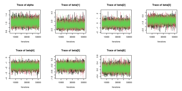
Figure 1: Trace plots for $\alpha$ and $\beta$’s of the AFT model (6).

Trace plots of the sampled values for each parameter in the chain appear overlapping one another and Gelman-Rubin values are very close to 1, which indicates that convergence has been achieved.

From the densplot function, also available from the coda package, we can draw the marginal posterior distributions (using kernel smoothing) for all the model parameters:

R> par(mfrow = c(2,4))
R> densplot(res, xlab = "")

Figure 2: Density plots for $\alpha$ and $\beta$’s of the AFT model (6).

Simulation-based Bayesian inference requires using simulated samples to summarise posterior distributions or calculate any relevant quantities of interest. So, posterior samples from the three Markov chains can be merged together using the following code:

R> result <- as.mcmc(do.call(rbind, res))

Next, the posterior samples of each parameter are extracted from the result object as follows:

R> alpha <- result[,1]; beta1 <- result[,2]; beta2 <- result[,3]; beta3 <- result[,4]
R> beta4 <- result[,5]; beta5 <- result[,6]; beta6 <- result[,7]

A relevant quantity for AFT models is the relative median (RM) between two individuals with covariate vectors ${\bm{x}}_{1}$ and ${\bm{x}}_{2}$. This measure compares the median of the survival time between both individuals and is defined as:

$$\mbox{RM}({\bm{x}}_{1},{\bm{x}}_{2},{\bm{\beta}})=\exp\left\{({\bm{x}}_{1}-{\bm{x}}_{2})^{\top}{\bm{\beta}}\right\}.$$

As an illustration, we can easily summarise the posterior distribution of the RM between two men of the same age and diagyr (year of diagnosis) but one in stage=3 and the other in stage=4:

R> RM.s3_s4 <- exp(beta3 - beta4)
R> summary(RM.s3_s4)
Iterations = 1:15000
Thinning interval = 1
Number of chains = 1
Sample size per chain = 15000

1. Empirical mean and standard deviation for each variable,
   plus standard error of the mean:
          Mean             SD       Naive SE Time-series SE
       3.01520        1.34859        0.01101        0.01179

2. Quantiles for each variable:
 2.5%   25%   50%   75% 97.5%
1.210 2.093 2.764 3.628 6.308

Proportional hazards models

The Cox proportional hazards model (Cox, 1972) expresses the hazard function $h(t)$ of the survival time of each individual of the target population as the product of a common baseline hazard function $h_{0}(t)$, which determines the shape of $h(t)$, and an exponential term which includes the relevant covariates ${\bm{x}}$ with regression coefficients $\bm{\beta}$ as follows:

$$h(t\mid h_{0},{\bm{\beta}})=h_{0}(t)\exp\left\{{\bm{x}}^{\top}{\bm{\beta}}\right\}.$$ (7)

The estimation of the regression coefficients in the Cox model under the frequentist approach can be obtained without specifying a model for the baseline hazard function by using partial likelihood methodology (Cox, 1972). This is not the case of Bayesian analysis which in general needs to specify some model for the baseline hazard (Christensen et al., 2011). Depending on the context of the study, baseline hazard misspecification can imply a loss of valuable model information that makes it impossible to fully report the estimation of the outcomes of interest, such as probabilities or survival curves for relevant covariate patterns (Royston, 2011). This is specially important in survival studies where $h_{0}(t)$ represents the natural course of a disease or an infection, or even the control group when comparing several treatments.

Baseline hazard functions can be defined through parametric or semi-parametric approaches. Parametric models give restricted shapes which do not allow the presence of irregular behaviour. Semi-parametric choices result in more flexible baseline hazard shapes that allow for multimodal patterns such as piecewise constant functions or spline functions. Theoretical and methodological aspects of more flexible approaches to define the baseline hazard function can be found in several specific references such as Ibrahim et al. (2001), Lin et al. (2015), Mitra and Müller (2015), Bogaerts et al. (2017), and Lázaro et al. (2020).

Model specification

The proportional hazards (PH) model implemented here is also illustrated with the larynx dataset (see Section 2.1). Survival time for each individual is modelled by means of the hazard function:

$$h(t\mid h_{0},{\bm{\beta}})=h_{0}(t)\exp\left\{\beta_{2}\mbox{I}_{(\texttt{stage}=2)}+\beta_{3}\mbox{I}_{(\texttt{stage}=3)}+\beta_{4}\mbox{I}_{(\texttt{stage}=4)}+\beta_{5}\texttt{age}+\beta_{6}\texttt{diagyr}\right\},$$ (8)

with baseline hazard function defined as a mixture of piecewise constant functions, $h_{0}(t\mid{\bm{\lambda}})=\sum_{k=1}^{K}\,\lambda_{k}\,I_{(a_{k-1},a_{k}]}(t)$, $t>0$, where ${\bm{\lambda}}=(\lambda_{1},\ldots,\lambda_{K})$ and $I_{(a_{k-1},a_{k}]}(t)$ is the indicator function defined as 1 when $t\in(a_{k-1},a_{k}]$ and 0 otherwise. We consider a total number of knots $K=3$ and an equally-spaced partition of the time axis from $a_{0}=0$ to $a_{4}=10.70$ which corresponds to the longest survival time observed. Prior scenario is set under a non-informative independent framework with a N($0,0.001$) for $\beta$’s and an independent gamma distributions, Ga($0.01,0.01$), for each $\lambda$.

Piecewise constant baseline hazard functions can accommodate different shapes of the hazard depending on the particular characteristics of the partition of the time axis (See Breslow (1974), Murray et al. (2016), and Lee et al. (2016) for different proposals in the subject). Similarly, there is a wide range of approaches to define marginal prior distributions for $h_{0}$ parameters, from prior independence to prior correlation. Correlated scenarios account for shape restrictions and also avoid overfitting and strong irregularities in the estimation process (Lázaro et al., 2020).

The likelihood function of this specific model is not implemented in JAGS, so the “zeros trick” approach using a Poisson distribution has been used to specify it indirectly (Ntzoufras, 2009; Lunn et al., 2012).

Model implementation

The variables age, diagyr, stage, and X are defined as in Section 2.1. In addition, as previously commented, piecewise constant is handled in JAGS considering the “zeros trick” (Ntzoufras, 2009; Lunn et al., 2012). To execute it, it is necessary to reformat the individual times (both observed and right-censored) to build an auxiliary variable (int.obs) that identifies the interval in which the $i$th individual experiences the event of interest. So, the following code is dedicated to define a time axis partition (i.e., intervals) and the int.obs variable:

R> # Time axis partition
R> K <- 3 # number of intervals
R> a <- seq(0, max(larynx$time) + 0.001, length.out = K + 1)
R> # int.obs: vector that tells us at which interval each observation is
R> int.obs <- matrix(data = NA, nrow = nrow(larynx), ncol = length(a) - 1)
R> d <- matrix(data = NA, nrow = nrow(larynx), ncol = length(a) - 1)
R> for(i in 1:nrow(larynx)){
+    for(k in 1:(length(a) - 1)){
+      d[i, k] <- ifelse(time[i] - a[k] > 0, 1, 0) * ifelse(a[k + 1] - time[i] > 0, 1, 0)
+      int.obs[i, k] <- d[i, k] * k
+    }
+  }
R> int.obs <- rowSums(int.obs)

Listing 2 shows a generic implementation of a PH piecewise constant model in BUGS syntax using larynx data.

Listing 2: PH model in BUGS syntax (file named as PH.txt).

⬇

1model{

2 for(i in 1:n){

3 for(k in 1:int.obs[i]){

4 cond[i,k] <- step(time[i] - a[k+1])

5 HH[i,k] <- cond[i,k] * (a[k+1]-a[k]) * lambda[k] +

6 (1-cond[i,k]) * (time[i]-a[k]) * lambda[k]

7 }

8 # Cumulative hazard function

9 H[i] <- sum(HH[i,1:int.obs[i]])

10 }

11 for(i in 1:n){

12 # Linear predictor

13 elinpred[i] <- exp(inprod(beta[],X[i,]))

14 # Log-hazard function

15 logHaz[i] <- log(lambda[int.obs[i]] * elinpred[i])

16 # Log-survival function

17 logSurv[i] <- -H[i] * elinpred[i]

18

19 # Definition of the log-likelihood using zeros trick

20 phi[i] <- 100000 - delta[i] * logHaz[i] - logSurv[i]

21 zeros[i] ~ dpois(phi[i])

22 }

23

24 # Prior distributions

25 for(l in 1:Nbetas){ beta[l] ~ dnorm(0,0.001) }

26 for(k in 1:m){ lambda[k] ~ dgamma(0.01,0.01) }

27}

Once the variables have been defined, a list with all the elements required in the model is created:

R> d.jags <- list(n = nrow(larynx), m = length(a) - 1, delta = larynx$delta,
+    time = larynx$time, X = X[,-1], a = a, int.obs = int.obs, Nbetas = ncol(X) - 1,
+    zeros = rep(0, nrow(larynx)))

The initial values for each PH model parameter are passed to JAGS using a function that returns a list of random values:

R> i.jags <- function(){ list(beta = rnorm(ncol(X) - 1), lambda = runif(3, 0.1)) }

The vector of monitored/saved parameters is:

R> p.jags <- c("beta", "lambda")

Next, the JAGS model is compiled:

R> library("rjags")
R> m2 <- jags.model(data = d.jags, file = "PH.txt", inits = i.jags, n.chains = 3)

We now run the model for 1000 burn-in simulations:

R> update(m2, 1000)

Finally, the model is run for 50000 additional simulations to keep one in 10 so that a proper thinning is done:

R> res <- coda.samples(m2, variable.names = p.jags, n.iter = 50000, n.thin = 10)

Similarly to the first example (Section 2.1), numerical and graphical summaries of the model parameters can be obtained using the summary and densplot functions, respectively. Gelman and Rubin’s convergence diagnostic can be calculated with the gelman.diag function, and the traceplot function provides a visual way to inspect sampling behaviour and assesses mixing across chains and convergence.

Next, simulations from the three Markov chains are merged together for inference:

R> result <- as.mcmc(do.call(rbind, res))

The posterior samples of each parameter are obtained by:

R> beta2 <- result[,1]; beta3 <- result[,2]; beta4 <- result[,3]; beta5 <- result[,4]
R> beta6 <- result[,5]; lambda1 <- result[,6]; lambda2 <- result[,7]; lambda3 <- result[,8]

Table 1 shows posterior summaries for the PH model parameters using larynx data.

Table 1: Posterior summaries for the PH model parameters.

Parameter	Mean	SD	$2.5\%$	$50\%$	$97.5\%$	$P(\cdot>0\mid\mbox{data})$
$\beta_{2}$ (stage=2)	0.152	0.474	-0.811	0.163	1.050	0.633
$\beta_{3}$ (stage=3)	0.672	0.363	-0.037	0.672	1.388	0.969
$\beta_{4}$ (stage=4)	1.804	0.443	0.924	1.809	2.659	1.000
$\beta_{5}$ (age)	0.215	0.155	-0.086	0.214	0.523	0.918
$\beta_{6}$ (diagyr)	-0.042	0.167	-0.368	-0.042	0.288	0.400
$\lambda_{1}$	0.069	0.021	0.035	0.066	0.116	1.000
$\lambda_{2}$	0.104	0.035	0.048	0.100	0.185	1.000
$\lambda_{3}$	0.079	0.064	0.008	0.062	0.246	1.000

The last column of Table 1 contains the posterior probability that the corresponding parameter is positive. A probability equal to $0.5$ indicates that a positive value of the parameter is equally likely than a negative one. Once we have the posterior sample of each parameter stored, the calculation of this posterior probability, for example for $\beta_{2}$, is given by mean(beta2>0).

A relevant quantity for PH models is the hazard ratio (HR), also called relative risk, between two individuals with covariate vectors ${\bm{x}}_{1}$ and ${\bm{x}}_{2}$. This measure is defined as:

$$\mbox{HR}({\bm{x}}_{1},{\bm{x}}_{2},h_{0},{\bm{\beta}})=\frac{h(t\mid{\bm{x}}_{1},h_{0},{\bm{\beta}})}{h(t\mid{\bm{x}}_{2},h_{0},{\bm{\beta}})}=\exp\left\{({\bm{x}}_{1}-{\bm{x}}_{2})^{\top}{\bm{\beta}}\right\},$$

and it is time independent. As an illustration, we can easily summarise the posterior distribution of the HR between two men of the same age and diagyr (year of diagnosis) but one in stage=3 and the other in stage=4:

R> HR.s3_s4 <- exp(beta3 - beta4)
R> summary(HR.s3_s4)
Iterations = 1:15000
Thinning interval = 1
Number of chains = 1
Sample size per chain = 15000

1. Empirical mean and standard deviation for each variable,
   plus standard error of the mean:
          Mean             SD       Naive SE Time-series SE
      0.354210       0.163810       0.001338       0.001338

2. Quantiles for each variable:
  2.5%    25%    50%    75%  97.5%
0.1384 0.2404 0.3217 0.4297 0.7667

Mixture cure models

Cure models

Cure models deal with target populations in which a part of the individuals cannot experience the event of interest. This type of models has widely been matured as a consequence of the discovery and development of new treatments against cancer. The rationale of considering a cure subpopulation comes from the idea that a successful treatment removes totally the original tumor and the individual cannot experience any recurrence of the disease. These models allow to estimate the probability of cure, a key and valuable outcome in cancer research.

Mixture cure models are the most popular cure models (Berkson and Gage, 1952). They consider the target population as a mixture of susceptible and non-susceptible individuals for the event of interest. Let $Z$ be a cure random variable defined as $Z=0$ for susceptible and $Z=1$ for cured or immune individuals. Cure and non cure probabilities are $P(Z=1)=\eta$ and $P(Z=0)=1-\eta$, respectively. The survival function for each individual in the cured and uncured subpopulation, $S_{c}(t)$ and $S_{u}(t)$, $t>0$, respectively, is

$$S_{u}(t)=P(T>t\mid Z=0),\;\;\;\;\;\;S_{c}(t)=P(T>t\mid Z=1),$$ (9)

and the general survival function for $T$ can be expressed as $S(t)=P(T>t)=\eta+(1-\eta)S_{u}(t)$. It is important to point out that $S_{u}(t)$ is a proper survival function but $S(t)$ is not. It goes to $\eta$ and not to zero when $t$ goes to infinity.

The effect of a baseline covariate vector ${\bm{x}}$ on the cure fraction $\eta$ for each individual is typically modelled by means of a logistic link function, logit$(\eta)$, but the probit link or the complementary log-log link could also be used. Covariates for modelling $T$ in the uncured subpopulation are usually considered via Cox models. Cure fraction model is usually known as the incidence model and the survival model (i.e., time-to-event $T$ in the uncured subpopulation) as the latency model Klein et al. (2013).

bmt dataset

We consider a bone marrow transplant dataset, referred to as bmt. It is available from the smcure package (Cai et al., 2012):

R> library("smcure")
R> data("bmt")
R> str(bmt)
’data.frame’:Ψ91 obs. of  3 variables:
 $ Time  : num  11 14 23 31 32 35 51 59 62 78 ...
 $ Status: num  1 1 1 1 1 1 1 1 1 1 ...
 $ TRT   : num  0 0 0 0 0 0 0 0 0 0 ...

This dataset refers to a bone marrow transplant study for the refractory acute lymphoblastic leukemia patients, in which 91 patients were divided into two treatment groups (Kersey et al., 1987). The following variables were observed for each patient:

• Time: time to death (in days).

• Status: censoring indicator (1: if patient is uncensored; 0: otherwise).

• TRT: treatment group indicator (0: allogeneic; 1: autologous).

Model specification

The (cure subpopulation) incidence model for each individual is expressed in terms of a logistic regression:

$$\mbox{logit}\big{[}\eta(\beta_{C1},\beta_{C2})\big{]}=\beta_{C1}+\beta_{C2}\texttt{TRT},$$ (10)

where $\beta_{C1}$ represents an intercept and $\beta_{C2}$ is the regression coefficient for the TRT covariate.

Survival time for each individual in the uncured subpopulation is modelled from a proportional hazards specification:

$$h_{u}(t\mid h_{0},\beta_{U})=h_{0}(t)\exp\left\{\beta_{U}\texttt{TRT}\right\},$$ (11)

with $h_{0}(t)=\lambda\,\alpha\,t^{\alpha-1}$ specified as a Weibull baseline hazard function, where $\alpha$ and $\lambda$ are the shape and scale parameters, respectively; and $\beta_{U}$ is the regression coefficient for the TRT covariate.

We assume prior independence and specify prior marginal distributions based on non-informative distributions commonly employed in the literature. The $\beta$’s follow a N($0,0.001$), while $\lambda$ and $\alpha$ follow a Gamma($0.01,0.01$) and a Un($0,10$), respectively.

The likelihood function for mixture cure models is not implemented in JAGS, so the “zeros trick” approach using a Poisson distribution has also been used to specify it indirectly (Ntzoufras, 2009; Lunn et al., 2012).

Model implementation

We have created two design matrices, one for model (10) and another for model (11), with the TRT covariate:

R> XC <- model.matrix(~ TRT, data = bmt) # Reference = allogeneic
R> XU <- model.matrix(~ TRT, data = bmt)
R> XU <- matrix(XU[,-1], ncol = 1) # Remove intercept

Listing 3 shows a generic implementation of a mixture cure model in BUGS syntax using bmt data.

Listing 3: Mixture cure model in BUGS syntax (file named as Cure.txt).

⬇

1model{

2 for(i in 1:n){

3 # Logistic regression model (cured subpopulation)

4 logit(eta[i]) <- inprod(betaC[],XC[i,])

5

6 # PH model (uncured subpopulation)

7 # Weibull baseline

8 base[i] <- lambda * alpha * pow(t[i],alpha-1)

9 elinpred[i] <- exp(inprod(betaU[],XU[i,]))

10 # Log-hazard function

11 logHaz[i] <- log(base[i] * elinpred[i])

12 # Log-survival function

13 logSurv[i] <- -lambda * pow(t[i],alpha) * elinpred[i]

14

15 # Definition of the log-likelihood using zeros trick

16 logLike[i] <- delta[i] * (log(1-eta[i]) + logHaz[i] + logSurv[i]) +

17 (1-delta[i]) * log(eta[i] + (1-eta[i]) * exp(logSurv[i]))

18 phi[i] <- 100000 - logLike[i]

19 zeros[i] ~ dpois(phi[i])

20 }

21

22 # Prior distributions

23 for(l in 1:NbetasC){ betaC[l] ~ dnorm(0,0.001) }

24 for(l in 1:NbetasU){ betaU[l] ~ dnorm(0,0.001) }

25 lambda ~ dgamma(0.01,0.01)

26 alpha ~ dunif(0,10)

27}

Once the variables have been defined, a list with all the elements required in the model is created:

R> d.jags <- list(n = nrow(bmt), t = bmt$Time, XC = XC, XU = XU,
+    delta = bmt$Status, zeros = rep(0, nrow(bmt)), NbetasC = ncol(XC), NbetasU = ncol(XU))

The initial values for each mixture cure model parameter are passed to JAGS using a function that returns a list of random values:

R> i.jags <- function(){
+    list(betaC = rnorm(ncol(XC)), betaU = rnorm(ncol(XU)), lambda = runif(1), alpha = runif(1))
+  }

The vector of monitored/saved parameters is:

R> p.jags <- c("betaC", "betaU", "alpha", "lambda")

Next, the JAGS model is compiled:

R> library("rjags")
R> m3 <- jags.model(data = d.jags, file = "Cure.txt", inits = i.jags, n.chains = 3)

We now run the model for 10000 burn-in simulations:

R> update(m3, 10000)

Finally, the model is run for 100000 additional simulations to keep one in 100 so that a proper thinning is done:

R> res <- coda.samples(m3, variable.names = p.jags, n.iter = 100000, n.thin = 100)

Similarly to the first example (Section 2.1), numerical and graphical summaries of the model parameters can be obtained using the summary and densplot functions, respectively. Gelman and Rubin’s convergence diagnostic can be calculated with the gelman.diag function, and the traceplot function provides a visual way to inspect sampling behaviour and assesses mixing across chains and convergence.

Next, simulations from the three Markov chains are merged together for inference:

R> result <- as.mcmc(do.call(rbind, res))

The posterior samples of each parameter are obtained by:

R> alpha <- result[,1]; betaC1 <- result[,2]; betaC2 <- result[,3]
R> betaU <- result[,4]; lambda <- result[,5]

Table 2 shows posterior summaries for the mixture cure model parameters using bmt data.

Table 2: Posterior summaries for the mixture cure model parameters.

Parameter	Mean	SD	$2.5\%$	$50\%$	$97.5\%$	$P(\cdot>0\mid\mbox{data})$
$\beta_{C1}$ (intercept)	-1.015	0.349	-1.731	-1.002	-0.365	0.001
$\beta_{C2}$ (TRT)	-0.419	0.519	-1.445	-0.417	0.591	0.208
$\beta_{U}$ (TRT)	0.762	0.269	0.239	0.760	1.294	0.998
$\alpha$	1.143	0.105	0.943	1.140	1.354	1.000
$\lambda$	0.002	0.001	0.000	0.002	0.006	1.000

As we discussed earlier, the cure fraction ($\eta$) is a relevant quantity for mixture cure models. For allogeneic (TRT=0) or autologous (TRT=1) treated patients, it is modelled as:

$$\eta(\texttt{TRT},\beta_{C1},\beta_{C2})=\frac{\exp(\beta_{C1}+\beta_{C2}\texttt{TRT})}{1+\exp(\beta_{C1}+\beta_{C2}\texttt{TRT})}.$$

We can easily summarise the posterior distribution of the cure fraction for individuals in both groups:

R> CP.allo <- exp(betaC1) / (1 + exp(betaC1))
R> CP.auto <- exp(betaC1 + betaC2) / (1 + exp(betaC1 + betaC2))
R> summary(cbind(CP.allo, CP.auto))
    CP.allo           CP.auto
 Min.   :0.01604   Min.   :0.02277
 1st Qu.:0.22426   1st Qu.:0.15680
 Median :0.26850   Median :0.19477
 Mean   :0.27146   Mean   :0.19925
 3rd Qu.:0.31515   3rd Qu.:0.23699
 Max.   :0.65573   Max.   :0.55898

The uncured survival curve based on posterior samples is another relevant information in this type of studies. So, from the posterior samples obtained above, we can summarise the posterior distribution of the mean value of the uncured survival curve for allogeneic and autologous treated patients in a grid of points as follows:

R> grid <- 100
R> time <- seq(0, bmt$Time, len = grid)
R> surv.allo <- surv.auto <- vector()
R> for(l in 1:grid){
+     surv.allo[l] <- mean(exp(-lambda * time[l]^alpha))
+     surv.auto[l] <- mean(exp(-lambda * exp(betaU) * time[l]^alpha))
+  }

Figure 3 shows the difference between both curves using the code below:

R> library("ggplot2")
R> treat.col <- rep(0:1, each = grid)
R> treat.col[treat.col == 0] <- "allogeneic"
R> treat.col[treat.col == 1] <- "autologous"
R> df <- data.frame(time = rep(time, 2), survival = c(surv.allo, surv.auto),
+    treatment = treat.col)
R> ggplot(data = df, aes(x = time, y = survival, group = treatment, colour = treatment)) +
+    geom_line() + theme_bw() + theme(legend.position = "top")

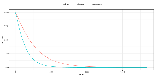
Figure 3: Posterior mean of the uncured survival function from the mixture cure model (11).

Competing risks models

Competing risks occur when the survival process includes more than one cause of failure. In the case of different causes of death it is only possible to report the first event to occur (Putter et al., 2007). There are different approaches for competing risk models: multivariate time to failure model, the cause-specific hazards model, the mixture model, the subdistribution model, and the full specified subdistribution model (Ge and Chen, 2012). We will only consider here the cause-specific hazards model, possibly the most popular of them.

Let $T_{k}$ be the random variable that represents the time-to-event from cause $k$, for $k=1,\ldots,K$, where $K$ is the total number of different events. The only survival time observed $T=\min\{T_{1},T_{2},\ldots,T_{K}\}$ usually corresponds to the earliest cause together with their indicator $\delta=k$ when the subsequent individual experiences the event due to cause $k$. The key concept in a competing risk model is the cause-specific hazard function for cause $k$, which assesses the hazard of experiencing the event $k$ in the presence of the rest of competing events, and it is defined by:

$$h_{k}(t)=\lim_{\Delta t\to 0}\frac{P(t\leq T<t+\Delta t,\delta=k\mid T\geq t)}{\Delta t}.$$ (12)

Inference for each $h_{k}(t)$ considers the observed failure times for cause $k$ as censored observations for the rest of events. Another relevant concept in the competing framework is the cumulative incidence function for cause $k$, defined as follows:

$$F_{k}(t)=P(T\leq t,\delta=k)=\int_{0}^{t}\,h_{k}(u)\,S(u)\,\mbox{d}u,$$ (13)

where $S(t)$ is the overall survival function. It is typically expressed in terms of the different cause-specific hazard functions in accordance with

$$S(t)=P(T>t)=\exp\Big{\{}-\sum_{k=1}^{K}\,\int_{0}^{t}\,h_{k}(u)\,\mbox{d}u\Big{\}}.$$

The cumulative incidence function is not a proper cumulative distribution function, i.e., the probability that the subsequent individual fails from cause $k$ is $F_{k}(\infty)=P(\delta=k)\neq 1$. The sub-survival function for cause $k$, defined as $S_{k}(t)=P(T>t,\delta=k)$, is also not a proper survival function.

okiss dataset

We consider a stem-cell transplanted patients dataset, referred to as okiss. It is available from the compeir package (Grambauer and Neudecker, 2011):

R> library("compeir")
R> data("okiss")
R> str(okiss)
’data.frame’:Ψ1000 obs. of  4 variables:
 $ time  : ’times’ num  21 6 14 12 11 18 10 8 17 10 ...
  ..- attr(*, "format")= chr "h:m:s"
 $ status: num  2 1 2 2 2 2 7 2 2 2 ...
 $ allo  : num  1 1 1 1 1 1 1 0 1 1 ...
 $ sex   : Factor w/ 2 levels "f","m": 1 1 1 2 2 2 2 1 2 2 ...

This dataset provides information about a sub-sample of 1000 patients enrolled in the ONKO-KISS programme, which is part of the German National Reference Centre for Surveillance of Hospital-Acquired Infections (Dettenkofer et al., 2005). These patients have been treated by peripheral blood stem-cell transplantation, which has become a successful therapy for severe hematologic diseases. After transplantation, patients are neutropenic, i.e., they have a low count of white blood cells, which are the cells that primarily avert infections (Beyersmann et al., 2007). Occurrence of bloodstream infection during neutropenia is a severe complication. The following variables were observed for each patient:

• time: time (in days) of neutropenia until first event.

• status: event status indicator (1: infection; 2: end of neutropenia; 7: death; 11: censored observation).

• allo: transplant type indicator (0: autologous; 1: allogeneic).

• sex: sex of each patient (m: if patient is male; f: if patient is female).

We have redefined the status variable using an auxiliary one (delta) in a matrix format:

R> delta <- matrix(c(as.integer(okiss$status == 1), as.integer(okiss$status == 2),
+    as.integer(okiss$status == 7)), ncol = 3)
R> head(delta)
     [,1] [,2] [,3]
[1,]    0    1    0
[2,]    1    0    0
[3,]    0    1    0
[4,]    0    1    0
[5,]    0    1    0
[6,]    0    1    0

where the events 1 (infection), 2 (end of neutropenia) and 7 (death) are indicated with a value of 1 in column 1, 2 or 3, respectively, and a row with only 0’s represents a censored observation.

Model specification

Cause-specific hazard functions for infection ($k=1$), end of neutropenia ($k=2$), and death ($k=3$) are modelled from a proportional hazard specification:

$$h_{k}(t\mid h_{0k},{\bm{\beta}}_{k})=h_{0k}(t)\exp\left\{\beta_{1k}\texttt{allo}+\beta_{2k}\texttt{sex}\right\},\;\;\;k=1,2,3,$$ (14)

with $h_{0k}(t)=\lambda_{k}\,\alpha_{k}\,t^{\alpha_{k}-1}$ for event $k$ specified as a Weibull baseline hazard function, where $\alpha_{k}$ and $\lambda_{k}$ are the shape and scale parameters, respectively; and ${\bm{\beta}}_{k}=(\beta_{1k},\beta_{2k})^{\top}$ are regression coefficients for the allo and sex covariates, respectively, for $k=1,2,3$. We assume prior independence and specify prior marginal based on non-informative distributions commonly employed in the literature. The $\beta$’s follow a N($0,0.001$), while $\lambda$’s and $\alpha$’s follow a Gamma($0.01,0.01$) and a Un($0,10$), respectively.

Model implementation

We have created a design matrix X with the covariates allo and sex:

R> X <- model.matrix(~ allo + sex, data = okiss) # Reference = female
R> X <- X[,-1] # Remove intercept

Listing 4 shows a generic implementation of a competing risks model in BUGS syntax using okiss data.

Listing 4: Competing risks model in BUGS syntax (file named as CR.txt).

⬇

1model{

2 for(i in 1:n){

3 for(k in 1:Nrisks){

4 # Weibull baseline

5 base[i,k] <- lambda[k] * alpha[k] * pow(t[i],alpha[k]-1)

6 elinpred[i,k] <- exp(inprod(beta[,k],X[i,]))

7 # Log-hazard functions

8 logHaz[i,k] <- log(base[i,k] * elinpred[i,k])

9 # Log-survival functions

10 logSurv[i,k] <- -lambda[k] * pow(t[i],alpha[k]) * elinpred[i,k]

11 }

12

13 # Definition of the log-likelihood using zeros trick

14 phi[i] <- 100000 - inprod(delta[i,],logHaz[i,]) - sum(logSurv[i,])

15 zeros[i] ~ dpois(phi[i])

16 }

17

18 # Prior distributions

19 for(k in 1:Nrisks){

20 for(l in 1:Nbetas){ beta[l,k] ~ dnorm(0,0.001) }

21 lambda[k] ~ dgamma(0.01,0.01)

22 alpha[k] ~ dunif(0,10)

23 }

24}

Once the variables have been defined, a list with all the elements required in the model is created:

R> d.jags <- list(n = nrow(okiss), t = as.vector(okiss$time), X = X,
+    delta = delta, zeros = rep(0, nrow(okiss)), Nbetas = ncol(X), Nrisks = ncol(delta))

The initial values for each competing risks model parameter are passed to JAGS using a function that returns a list of random values:

R> i.jags <- function(){
+    list(beta = matrix(rnorm(ncol(X) * ncol(delta)), ncol = ncol(delta)),
+      lambda = runif(ncol(delta)), alpha = runif(ncol(delta)))
+  }

The vector of monitored/saved parameters is:

R> p.jags <- c("beta", "alpha", "lambda")

Next, the JAGS model is compiled:

R> library("rjags")
R> m4 <- jags.model(data = d.jags, file = "CR.txt", inits = i.jags, n.chains = 3)

We now run the model for 1000 burn-in simulations:

R> update(m4, 1000)

Finally, the model is run for 10000 additional simulations to keep one in 10 so that a proper thinning is done:

R> res <- coda.samples(m4, variable.names = p.jags, n.iter = 10000, n.thin = 10)

Similarly to the first example (Section 2.1), numerical and graphical summaries of the model parameters can be obtained using the summary and densplot functions, respectively. Gelman and Rubin’s convergence diagnostic can be calculated with the gelman.diag function, and the traceplot function provides a visual way to inspect sampling behaviour and assesses mixing across chains and convergence.

Next, simulations from the three Markov chains are merged together for inference:

R> result <- as.mcmc(do.call(rbind, res))

The posterior samples of each parameter are obtained by:

R> alpha1 <- result[,1]; alpha2 <- result[,2]; alpha3 <- result[,3]; beta11 <- result[,4]
R> beta21 <- result[,5]; beta12 <- result[,6]; beta22 <- result[,7]; beta13 <- result[,8]
R> beta23 <- result[,9]; lambda1 <- result[,10]; lambda2 <- result[,11]; lambda3 <- result[,12]

Table 3 shows posterior summaries for the competing risks model parameters using okiss data.

Table 3: Posterior summaries for the competing risks model parameters.

Parameter	Mean	SD	$2.5\%$	$50\%$	$97.5\%$	$P(\cdot>0\mid\mbox{data})$
Infection ($h_{1}$)
$\beta_{11}$ (allo)	-0.523	0.151	-0.817	-0.523	-0.225	0.000
$\beta_{21}$ (sex)	0.158	0.148	-0.130	0.156	0.451	0.857
$\lambda_{1}$	0.014	0.003	0.009	0.014	0.022	1.000
$\alpha_{1}$	1.137	0.070	1.003	1.136	1.278	1.000
End of neutropenia ($h_{2}$)
$\beta_{12}$ (allo)	-1.193	0.075	-1.340	-1.193	-1.046	0.000
$\beta_{22}$ (sex)	-0.102	0.073	-0.244	-0.103	0.042	0.081
$\lambda_{2}$	0.008	0.001	0.006	0.008	0.010	1.000
$\alpha_{2}$	2.033	0.045	1.947	2.034	2.120	1.000
Death ($h_{3}$)
$\beta_{13}$ (allo)	-0.617	0.747	-2.001	-0.650	0.945	0.193
$\beta_{23}$ (sex)	0.446	0.730	-0.859	0.408	1.986	0.718
$\lambda_{3}$	0.000	0.000	0.000	0.000	0.000	1.000
$\alpha_{3}$	2.628	0.418	1.813	2.623	3.466	1.000

As discussed in Section 4, the cumulative incidence function $F_{k}(t)$ in ( 13) is the most appropriate way to analyse the evolution of each cause $k$ over time. For our proportional hazard specification (14), it is given by:

$$F_{k}(t)=\int_{0}^{t}\,h_{k}(t\mid h_{0k},{\bm{\beta}}_{k})\,\exp\Big{\{}-\sum_{l=1}^{3}\int_{0}^{u}\,h_{l}(v\mid h_{0l},{\bm{\beta}}_{l})\,\mbox{d}v\Big{\}}\,\mbox{d}u,$$ (15)

where $h_{k}(t\mid h_{0k},{\bm{\beta}}_{k})$ is defined in (14).

The integral in (15) has no closed form, so some approximate method of integration is required. To do this, we first have created a function fk which describes the integrand of (15):

R> fk <- function(u.vect, lambda, alpha, beta, x, k){
+  res <- sapply(u.vect, function(u){
+    # Cause-specific hazard
+    hk <- lambda[k] * alpha[k] * (u^(alpha[k] - 1)) * exp(sum(unlist(beta[,k]) * x))
+    # Cumulative cause-specific hazard
+    Hk <- lambda * (rep(u, length(lambda))^alpha) * exp((t(beta) %*% matrix(x, ncol = 1))[,1])
+    # Cause-specific hazard x Overall survival
+    aux <- hk * exp(-sum(Hk))
+    return(aux)
+  })
+  return(res) }

Next, we have created a function cif that computes $F_{k}(t)$ in (15) by integrating out the fk function using the integral function available from the pracma package (Borchers, 2019).

R> library("pracma")
R> cif <- function(tt, lambda, alpha, beta, x, k){
+    return(integral(fk, xmin = 0, xmax = tt, method = "Simpson", lambda = lambda, alpha = alpha,
+      beta = beta, x = x, k = k)) }

Finally, we have constructed a function mcmc$\_$cif that takes the output from JAGS (variable obj) and computes $F_{k}(t)$ in (15) for a vector of times (variable t.pred) using covariates x. Note that mcmc$\_$cif is based on the mclapply function, available from the parallel package to speed computations up (R Core Team, 2020).

R> library("parallel")
R> options(mc.cores = detectCores())
R> mcmc_cif <- function(obj, t.pred, x){
+    var.names <- names(obj)
+    # Indices of beta’s, alpha’s, and lambda’s
+    b.idx <- which(substr(var.names, 1, 4) == "beta")
+    a.idx <- which(substr(var.names, 1, 5) == "alpha")
+    l.idx <- which(substr(var.names, 1, 6) == "lambda")
+    # Number of causes and number of covariates
+    K <- length(a.idx)
+    n.b <- length(b.idx) / K
+    # Sub-sample to speed up computations
+    samples.idx <- sample(1:nrow(obj), 200)
+
+    res <- lapply(1:K, function(k){
+      sapply(t.pred, function(tt){
+        aux <- mclapply(samples.idx, function(i){
+          cif(tt, alpha = unlist(obj[i, a.idx]), lambda = unlist(obj[i, l.idx]),
+             beta = matrix(unlist(c(res[i, b.idx])), nrow = n.b), x = x, k = k)
+        })
+        return(mean(unlist(aux)))
+      })
+    })
+    return(res)
+  }

Hence, we redefine the MCMC output as a data.frame and set a vector of times to evaluate the cumulative incidence function. In this example, we are interested in this function when both covariates are 1 (i.e., allogeneic transplant and male).

R> res <- as.data.frame(result)
R> t.pred <- seq(0, 100, by = 2.5)
R> cum_inc <- mcmc_cif(res, t.pred, c(1, 1))

Figure 4, generated with the code below, shows the posterior mean of the cumulative incidence function for a man with an allogeneic transplant for the three types of events considered in the okiss data.

R> library("ggplot2")
R> df <- data.frame(cif = unlist(cum_inc), time = t.pred,
+    cause = rep(c("infection", "end of neutropenia", "death"), each = length(t.pred)))
R> ggplot(data = df, aes(x = time, y = cif, group = cause)) + geom_line(aes(color = cause)) +
+    ylab("cumulative incidence") + ylim(c(0,1)) + theme_bw() + theme(legend.position = "top")

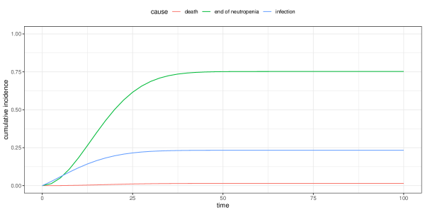
Figure 4: Posterior mean of the cumulative incidence function for allo=1 (allogeneic transplant) and sex=1 (male) from the competing risks model (14).

Multi-state models

Multi-state models are a class of stochastic processes which account for event history data, with individuals who may experience different events in time. Relevant data are the events and their subsequent survival times. Multi-state models allow for different structures depending on the number and relationships between the states (Andersen and Keiding, 2002). Outputs of interest are the usual in survival analysis (sometimes with a specific vocabulary, e.g., the hazard function which is now called transition intensity) to which transition probabilities are added.

We concentrate on the illness-death model (also known as disability model) which is a particular multi-state model. This is a relevant model in irreversible diseases where a significant illness’ progression increases the risk of a terminal event (Han et al., 2014; Armero et al., 2016a). The underlying stochastic process $\{Z(t),t\geq 0\}$ describes the state of an individual at time $t$, where $t$ is time from entry into the initial state (state 1). The probabilistic behaviour of the process is determined by the subsequent hazard functions from which transitions probabilities between states, defined as $p_{jk}(s,t\mid\bm{\theta})=P(Z(t)=k\mid Z(s)=j,\bm{\theta})$, can be derived, where $s\leq t$, $j$ and $k$ are states, $\sum_{j=k}^{3}\,p_{jk}(s,t\mid\bm{\theta})=1$, for $k=1,2,3$, and $\bm{\theta}$ is the vector of model parameters.

Each transition has its respective hazard function, for example, $h_{12}(t\mid\bm{\theta})$ is associated with time $T_{12}$ from state 1 to state 2 (1 $\rightarrow$ 2), while $h_{13}(t\mid\bm{\theta})$ and $h_{23}(t\mid\bm{\theta})$ represent the hazard functions for the time $T_{13}$ (1 $\rightarrow$ 3) and $T_{23}$ (2 $\rightarrow$ 3), respectively. If $h_{23}(t\mid\bm{\theta})$ does not depend of the time in which transition 1 $\rightarrow$ 2 occurs, the process will be known as Markovian. Otherwise, it is called semi-Markovian and transition probabilities 2 $\rightarrow$ 3 will depend on the particular value of $T_{12}$.

Transition probabilities between states and hazard functions for the semi-Markovian specification are connected as follows (Andersen and Perme, 2008):

$$p_{11}(s,t\mid\bm{\theta}) = \exp\Bigg{\{}-\int_{s}^{t}\left[h_{12}(u\mid\bm{\theta})+h_{13}(u\mid\bm{\theta})\right]\mbox{d}u\Bigg{\}},$$ (16)

$$p_{22}(s,t\mid\bm{\theta},t_{12}) = \exp\Bigg{\{}-\int_{s}^{t}\,h_{23}(u-t_{12}\mid\bm{\theta},t_{12})\;\mbox{d}u\Bigg{\}},\;\;\;t_{12}<s,$$ (17)

$$p_{12}(s,t\mid\bm{\theta}) = \int_{s}^{t}\,p_{11}(s,u\mid\bm{\theta})\,h_{12}(u\mid\bm{\theta})\,p_{22}(u,t\mid\bm{\theta},u)\;\mbox{d}u,$$ (18)

$$p_{13}(s,t\mid\bm{\theta}) = 1-p_{11}(s,t\mid\bm{\theta})-p_{12}(s,t\mid\bm{\theta}),$$ (19)

$$p_{23}(s,t\mid\bm{\theta}) = 1-p_{22}(s,t\mid\bm{\theta}),$$ (20)

$$p_{33}(s,t\mid\bm{\theta}) = 1,$$ (21)

where the marginal probability $p_{22}(s,t\mid\bm{\theta})$ is obtained by integrating out $p_{22}(s,t\mid\bm{\theta},t_{12})$ with regard to the density of $T_{12}$ from 0 to $s$.

The standard specification of an illness-death model is through the hazard function of the relevant survival times, generally modelled by means of Cox models. Consequently, the specification of prior distributions for $\bm{\theta}$ must be addressed to them in Section 2.2.

heart2 dataset

We consider a heart transplant dataset, referred to as heart2. It is available from the p3state.msm package (Meira-Machado and Roca-Pardinas, 2012):

R> library("p3state.msm")
R> data("heart2")
R> str(heart2)
’data.frame’:Ψ103 obs. of  8 variables:
 $ times1 : num  50 6 1 36 18 3 51 40 85 12 ...
 $ delta  : int  0 0 1 1 0 0 1 0 0 1 ...
 $ times2 : num  0 0 15 3 0 0 624 0 0 46 ...
 $ time   : int  50 6 16 39 18 3 675 40 85 58 ...
 $ status : int  1 1 1 1 1 1 1 1 1 1 ...
 $ age    : num  -17.16 3.84 6.3 -7.74 -27.21 ...
 $ year   : num  0.123 0.255 0.266 0.49 0.608 ...
 $ surgery: int  0 0 0 0 0 0 0 0 0 0 ...

This dataset provides information about a sample of 103 patients of the Stanford Heart Transplant Program (Crowley and Hu, 1977). The patients are initially on the waiting list (state 1) and can either be transplanted (state 2, non-terminal event) and then die (state 3, terminal event), or just one or none of them because they continue to be on the waiting list. The following variables were observed for each patient:

• times1: time of transplant/censoring time (state 2).

• delta: transplant indicator (1: yes; 0: no).

• times2: time to death since the transplant/censoring time (state 3).

• time: times1 + times2.

• status: censoring indicator (1: dead; 0: alive).

• age: age - 48 years.

• year: year of acceptance (in years after 1 Nov 1967).

• surgery: prior bypass surgery (1: yes; 0: no).

The patients had the following characteristics: 4 were censored for both events (transplant and death), 24 moved from state 1 (waiting list) to state 2 (transplant) and survived, 30 moved from state 1 to state 3 (death) without going through state 2, and 45 moved from state 1 to state 2 and then to state 3.

We have redefined delta and status variables using an auxiliary one (event) in a matrix format:

R> event <- matrix(c(heart2$delta, heart2$status * (1 - heart2$delta),
+    heart2$delta * heart2$status), ncol = 3)
R> head(event)
     [,1] [,2] [,3]
[1,]    0    1    0
[2,]    0    1    0
[3,]    1    0    1
[4,]    1    0    1
[5,]    0    1    0
[6,]    0    1    0

where each row represents the transitions of a patient, in which a 1 in columns 1, 2 and 3 indicates transition 1 $\rightarrow$ 2, 1 $\rightarrow$ 3, and 2 $\rightarrow$ 3, respectively, and a row with only 0’s represents a censored observation.

Model specification

Hazard functions for survival times $T_{12}$, $T_{13}$ and $T_{23}$ are modelled using a proportional hazard specification:

$$h_{12}(t\mid h_{01},{\bm{\beta}}_{1}) = h_{01}(t)\exp\left\{\beta_{11}\texttt{age}+\beta_{21}\texttt{year}+\beta_{31}\texttt{surgery}\right\},\;\;\;t>0,$$ (22)

$$h_{13}(t\mid h_{02},{\bm{\beta}}_{2}) = h_{02}(t)\exp\left\{\beta_{12}\texttt{age}+\beta_{22}\texttt{year}+\beta_{32}\texttt{surgery}\right\},\;\;\;t>0,$$ (23)

$$h_{23}(t\mid h_{03},{\bm{\beta}}_{3},T_{12}=t_{12}) = h_{03}(t-t_{12})\exp\left\{\beta_{13}\texttt{age}+\beta_{23}\texttt{year}+\beta_{33}\texttt{surgery}\right\},\;\;\;t>t_{12},$$ (24)

with $h_{0k}(t)=\lambda_{k}\alpha_{k}t^{\alpha_{k}-1}$ specified as a Weibull baseline hazard function, where $\alpha_{k}$ and $\lambda_{k}$ are the shape and scale parameters, respectively, for $k=1,2,3$; and ${\bm{\beta}}_{k}=(\beta_{1k},\beta_{2k},\beta_{3k})^{\top}$ are regression coefficients for the age, year and surgery covariates, respectively, We assume prior independence and specify prior marginal based on non-informative distributions commonly employed in the literature. The $\beta$’s follow a N($0,0.001$), while $\lambda$’s and $\alpha$’s follow a Gamma($0.01,0.01$) and a Un($0,10$), respectively. Note that in (24) we adopt the semi-Markovian specification, but it could also be the Markovian one (Alvares et al., 2019).

Model implementation

We have created a design matrix X with the covariates age, year and surgery, and defined a time3 $=t-t_{12}$ variable according to semi-Markovian specification:

R> X <- model.matrix(~ age + year + surgery, data = heart2)
R> X <- X[,-1] # Remove intercept
R> time3 <- heart2$times2
R> time3[time3 == 0] <- 0.0001

The values of time3 equal to zero have been replaced by 0.0001 to avoid computational problems when calculating $(t-t_{12})^{\alpha_{3}-1}$.

Listing 5 shows a generic implementation of an illness-death model in BUGS syntax using heart2 data.

Listing 5: Illness-death model in BUGS syntax (file named as IllDeath.txt).

⬇

1model{

2 for(i in 1:n){

3 # Linear predictor

4 elinpred[i,1] <- exp(inprod(beta[,1],X[i,]))

5 elinpred[i,2] <- exp(inprod(beta[,2],X[i,]))

6 elinpred[i,3] <- exp(inprod(beta[,3],X[i,]))

7 # Log-hazard functions

8 logHaz[i,1] <- log(lambda[1] * alpha[1] * pow(t1[i],alpha[1]-1) * elinpred[i,1])

9 logHaz[i,2] <- log(lambda[2] * alpha[2] * pow(t2[i],alpha[2]-1) * elinpred[i,2])

10 logHaz[i,3] <- log(lambda[3] * alpha[3] * pow(t3[i],alpha[3]-1) * elinpred[i,3])

11 # Log-survival functions

12 logSurv[i,1] <- -lambda[1] * pow(t1[i],alpha[1]) * elinpred[i,1]

13 logSurv[i,2] <- -lambda[2] * pow(t2[i],alpha[2]) * elinpred[i,2]

14 logSurv[i,3] <- -lambda[3] * pow(t3[i],alpha[3]) * elinpred[i,3]

15

16 # Definition of the log-likelihood using zeros trick

17 phi[i] <- 100000 - inprod(event[i,],logHaz[i,]) - sum(logSurv[i,])

18 zeros[i] ~ dpois(phi[i])

19 }

20

21 # Prior distributions

22 for(k in 1:3){

23 for(l in 1:Nbetas){ beta[l,k] ~ dnorm(0,0.001) }

24 lambda[k] ~ dgamma(0.01,0.01)

25 alpha[k] ~ dunif(0,10)

26 }

27}

Once the variables have been defined, a list with all the elements required in the model is created:

R> d.jags <- list(n = nrow(heart2), t1 = heart2$times1, t2 = heart2$time, t3 = time3,
+    X = X, event = event, zeros = rep(0, nrow(heart2)), Nbetas = ncol(X))

The initial values for each illness-death model parameter are passed to JAGS using a function that returns a list of random values:

R> i.jags <- function(){
+    list(beta = matrix(rnorm(3 * ncol(X)), ncol = 3), lambda = runif(3), alpha = runif(3))
+  }

The vector of monitored/saved parameters is:

R> p.jags <- c("beta", "alpha", "lambda")

Next, the JAGS model is compiled:

R> library("rjags")
R> m5 <- jags.model(data = d.jags, file = "IllDeath.txt", inits = i.jags, n.chains = 3)

We now run the model for 1000 burn-in simulations:

R> update(m5, 1000)

Finally, the model is run for 10000 additional simulations to keep one in 10 so that a proper thinning is done:

R> res <- coda.samples(m5, variable.names = p.jags, n.iter = 10000, n.thin = 10)

Similarly to the first example (Section 2.1), numerical and graphical summaries of the model parameters can be obtained using the summary and densplot functions, respectively. Gelman and Rubin’s convergence diagnostic can be calculated with the gelman.diag function, and the traceplot function provides a visual way to inspect sampling behaviour and assesses mixing across chains and convergence.

Next, simulations from the three Markov chains are merged together for inference:

R> result <- as.mcmc(do.call(rbind, res))

The posterior samples of each parameter are obtained by:

R> alpha1 <- result[,1]; alpha2 <- result[,2]; alpha3 <- result[,3]
R> beta11 <- result[,4]; beta21 <- result[,5]; beta31 <- result[,6]
R> beta12 <- result[,7]; beta22 <- result[,8]; beta32 <- result[,9]
R> beta13 <- result[,10]; beta23 <- result[,11]; beta33 <- result[,12]
R> lambda1 <- result[,13]; lambda2 <- result[,14]; lambda3 <- result[,15]

Table 4 shows posterior summaries for the illness-death model parameters using heart2 data.

Table 4: Posterior summaries for the illness-death model parameters.

Parameter	Mean	SD	$2.5\%$	$50\%$	$97.5\%$	$P(\cdot>0\mid\mbox{data})$
From waiting list to heart transplant ($h_{12}$)
$\beta_{11}$	0.048	0.015	0.020	0.047	0.077	1.000
$\beta_{21}$	0.004	0.069	-0.130	0.004	0.140	0.521
$\beta_{31}$	0.220	0.321	-0.440	0.229	0.826	0.760
$\lambda_{1}$	0.042	0.016	0.018	0.039	0.079	1.000
$\alpha_{1}$	0.778	0.069	0.645	0.777	0.916	1.000
From waiting list to death ($h_{13}$)
$\beta_{12}$	-0.001	0.018	-0.034	-0.002	0.035	0.462
$\beta_{22}$	-0.243	0.115	-0.476	-0.241	-0.027	0.013
$\beta_{32}$	-0.785	0.672	-2.223	-0.736	0.391	0.109
$\lambda_{2}$	0.101	0.047	0.034	0.092	0.217	1.000
$\alpha_{2}$	0.379	0.058	0.272	0.376	0.500	1.000
From heart transplant to death ($h_{23}$)
$\beta_{13}$	0.055	0.022	0.014	0.055	0.099	0.997
$\beta_{23}$	-0.008	0.094	-0.196	-0.007	0.174	0.470
$\beta_{33}$	-0.986	0.469	-1.973	-0.961	-0.129	0.011
$\lambda_{3}$	0.034	0.021	0.008	0.029	0.087	1.000
$\alpha_{3}$	0.602	0.074	0.463	0.598	0.756	1.000

As discussed in Section 5, the transition probabilities (16)–(21) are the most appropriate way to analyse the evolution of each state over time. The implementation of the posterior distribution for these transition probabilities requires auxiliary functions, similar to the calculation of the cumulative incidence function in Section 4. To avoid unnecessary repetitions on how to calculate these quantities of interest, we will omit their implementation here. However, the code to reproduce Figure 5 is available in Appendix A.

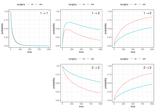
Figure 5: Posterior mean of all probability transitions from the illness-death model (22)–(24) for patients with and without prior bypass surgery and median values of age and year. Graphics on the top correspond to transitions from the initial state in the waiting list. Posterior probabilities for transitions from transplant (bottom row) assume the median time $T_{12}=26$ recorded from the waiting list to heart transplant.

Frailty models

Regression models include measurable covariates to improve the knowledge of the relevant failure times. However, in most survival studies, there are also individual heterogeneity that are not known or measurable. These elements are known in the statistical framework as random effects, but in the context of survival models they are the frailty elements (Aalen, 1994). They can approach individual characteristics as well as heterogeneity in groups or clusters (Ibrahim et al., 2001).

The most popular type of frailty models is the multiplicative shared-frailty model. It is a generalisation of the Cox regression model introduced by Clayton (1978) and extensively studied in Hougaard (2000). Let $T_{i}$ the survival time for each individual in group $i$ with hazard function described by:

$$h_{i}(t\mid h_{0},{\bm{\beta}},w_{i})=w_{i}\,h_{0}(t)\exp\left\{{\bm{x}_{i}}^{\top}{\bm{\beta}}\right\},$$ (25)

where $w_{i}$ is the frailty term associated to group $i$. The usual probabilistic model for the frailty term is a gamma distribution with mean equal to one for identifiability purposes but also the positive stable and log-normal distributions can be considered (Vaupel et al., 1979). In addition, a unity mean can be considered as a neutral frontier because frailty values greater (lower) than one increases (decreases) the individual risk. An alternative way of incorporating a frailty term in the hazard function is via an additive element as follows:

$$h_{i}(t\mid h_{0},{\bm{\beta}},b_{i})=h_{0}(t)\exp\left\{{\bm{x}_{i}}^{\top}{\bm{\beta}}+b_{i}\right\},$$

where now $b_{i}$’s are commonly assumed as normally distributed with zero mean and unknown variance.

The Bayesian framework deals with frailty models in a conceptually simpler way than the frequentist one due to the Bayesian probability conception, introduced in Section 1. Hence, the inclusion of randomness through frailties in a Bayesian perspective does not add any conceptual complexity because the information regarding the risk function is expressed in probabilistic terms through its posterior distribution. Survival modelling with frailty terms is a wide issue of research that applies to all type of regression, competing risks, multivariate survival models, etc. and play a special role in joint models as we will discuss later.

kidney dataset

We consider a kidney infection dataset, referred to as kidney. It is available from the frailtyHL package (Ha et al., 2018):

R> library("frailtyHL")
R> data("kidney")
R> str(kidney)
’data.frame’:Ψ76 obs. of  10 variables:
 $ id     : num  1 1 2 2 3 3 4 4 5 5 ...
 $ time   : num  8 16 23 13 22 28 447 318 30 12 ...
 $ status : num  1 1 1 0 1 1 1 1 1 1 ...
 $ age    : num  28 28 48 48 32 32 31 32 10 10 ...
 $ sex    : num  1 1 2 2 1 1 2 2 1 1 ...
 $ disease: Factor w/ 4 levels "Other","GN","AN",..: 1 1 2 2 1 1 1 1 1 1 ...
 $ frail  : num  2.3 2.3 1.9 1.9 1.2 1.2 0.5 0.5 1.5 1.5 ...
 $ GN     : num  0 0 1 1 0 0 0 0 0 0 ...
 $ AN     : num  0 0 0 0 0 0 0 0 0 0 ...
 $ PKD    : num  0 0 0 0 0 0 0 0 0 0 ...

This dataset consists of times to the first and second recurrences of infection in 38 kidney patients using a portable dialysis machine. Infections can occur at the location of insertion of the catheter. The catheter is later removed if infection occurs and can be removed for other reasons, in which case the observation is censored (McGilchrist and Aisbett, 1991). The following variables were repeated twice for each patient:

• id: patient number.

• time: time (in days) from insertion of the catheter to infection in kidney patients using portable dialysis machine.

• status: censoring indicator (1: if patient is uncensored; 0: otherwise).

• age: age (in years) of each patient.

• sex: sex of each patient (1: if patient is male; 2: if patient is female).

• disease: disease type (GN; AN; PKD; Other).

• frail: frailty estimate from original paper.

• GN: indicator for disease type GN.

• AN: indicator for disease type AN.

• PKD: indicator for disease type PKD.

Note that the status variable equal to zero in any of the recurrences means that until that moment of observation there was no infection. We would also like to mention that we will use a modelling based on the clock-reset approach (Kleinbaum and Klein, 2012), in which time starts at zero again after each recurrence.

Model implementation

Time, in days, from insertion of a catheter in patient $i$th to infection is modelled trough a proportional hazard specification with multiplicative frailties:

$$h_{i}(t\mid h_{0},{\bm{\beta}},w_{i})=w_{i}\,h_{0}(t)\exp\left\{\beta_{2}\texttt{sex}\right\},$$ (26)

where $w_{i}\sim\mbox{Gamma}(\psi,\psi)$ represents the frailty term for each individual; $h_{0}(t)=\lambda\,\alpha\,t^{\alpha-1}$ is specified as a Weibull baseline hazard function, where $\alpha$ and $\lambda=\exp(\beta_{1})$ are the shape and scale parameters, respectively; and $\beta_{2}$ is the regression coefficient for the sex covariate. As the purpose of this modelling is illustrative, the other covariates will not be considered. We assume prior independence and specify prior marginal based on non-informative distributions commonly employed in the literature. The $\beta$’s follow a N($0,0.001$), while $\alpha$ and $\psi$ follow a Un($0,10$) and a Gamma($0.01,0.01$), respectively.

Our variable of interest is time, which represents the time from insertion of the catheter to infection. The status covariate plays an important role in the codification of the survival and censoring times:

R> # Number of patients and catheters
R> n <- length(unique(kidney$id))
R> J <- 2
R> # Survival and censoring times
R> time <- kidney$time
R> cens <- time
R> time[kidney$status == 0] <- NA # Censored
R> is.censored <- as.numeric(is.na(time))
R> # Matrix format
R> time <- matrix(time, n, J, byrow = TRUE)
R> cens <- matrix(cens, n, J, byrow = TRUE)
R> is.censored <- matrix(is.censored, n, J, byrow = TRUE)

Without loss of generality, we have created a design matrix X with the sex covariate:

R> sex <- kidney$sex[seq(1, 2 * n, 2)] - 1 # Reference = male
R> X <- model.matrix(~ sex)

Listing 6 shows a generic implementation of a frailty model in BUGS syntax using kidney data.

Listing 6: Frailty model in BUGS syntax (file named as Frailty.txt).

⬇

1model{

2 for(i in 1:n){

3 for(j in 1:J){

4 # Survival and censoring times

5 is.censored[i,j] ~ dinterval(time[i,j],cens[i,j])

6 time[i,j] ~ dweib(alpha,lbd[i,j])

7 log(lbd[i,j]) <- inprod(beta[],X[i,]) + log(w[i])

8 }

9 # Multiplicative frailties

10 w[i] ~ dgamma(psi,psi)

11 }

12

13 # Prior distributions

14 for(l in 1:Nbetas){ beta[l] ~ dnorm(0.0,0.001) }

15 alpha ~ dunif(0,10)

16 psi ~ dgamma(0.01,0.01)

17

18 # Derived quantity

19 lambda <- exp(beta[1])

20}

Model estimation: JAGS from R

Once the variables have been defined, a list with all the elements required in the model is created:

R> d.jags <- list(n = n, J = J, time = time, cens = cens, X = X,
+   is.censored = is.censored, Nbetas = ncol(X))

The initial values for each frailty model parameter are passed to JAGS using a function that returns a list of random values:

R> i.jags <- function(){ list(beta = rnorm(ncol(X)), alpha = runif(1), psi = runif(1)) }

The vector of monitored/saved parameters is:

R> p.jags <- c("beta", "alpha", "lambda", "psi", "w")

Next, the JAGS model is compiled:

R> library("rjags")
R> m6 <- jags.model(data = d.jags, file = "Frailty.txt", inits = i.jags, n.chains = 3)

We now run the model for 10000 burn-in simulations:

R> update(m6, 10000)

Finally, the model is run for 100000 additional simulations to keep one in 100 so that a proper thinning is done:

R> res <- coda.samples(m6, variable.names = p.jags, n.iter = 100000, thin = 100)

Similarly to the first example (Section 2.1), numerical and graphical summaries of the model parameters can be obtained using the summary and densplot functions, respectively. Gelman and Rubin’s convergence diagnostic can be calculated with the gelman.diag function, and the traceplot function provides a visual way to inspect sampling behaviour and assesses mixing across chains and convergence.

Next, simulations from the three Markov chains are merged together for inference:

R> result <- as.mcmc(do.call(rbind, res))

The posterior samples of each parameter are obtained by:

R> alpha <- result[,1]; beta2 <- result[,3]; lambda <- result[,4]
R> psi <- result[,5]; w <- result[,6:ncol(result)]

Table 5 shows posterior summaries for the frailty model parameters using kidney.

Table 5: Posterior summaries for the frailty model parameters.

Parameter	Mean	SD	$2.5\%$	$50\%$	$97.5\%$	$P(\cdot>0\mid\mbox{data})$
$\beta_{2}$ (sex)	-1.908	0.555	-3.064	-1.889	-0.876	0.000
$\alpha$	1.233	0.167	0.929	1.222	1.592	1.000
$\lambda$	0.019	0.012	0.004	0.017	0.050	1.000
$\psi$	2.417	2.101	0.779	1.878	7.844	1.000

The individual survival curve based on posterior samples is a relevant information in this type of studies. So, we can summarise the posterior distribution of the individual survival curve in a grid of points as follows:

R> grid <- 1000
R> time <- seq(0, max(kidney$time), len = grid)
R> surv <- matrix(NA, n, grid)
R> for(i in 1:n){
+    for(k in 1:grid){
+       surv[i, k] <- mean(exp(-w[i] * lambda * exp(beta2 * sex[i]) * time[k]^alpha))
+    }
+  }

Next, we can differentiate the survival curves by sex (code below). Figure 6 shows such curves for all patients in the kidney data.

R> library("ggplot2")
R> sex.col <- sex
R> sex.col[sex == 0] <- "male"
R> sex.col[sex == 1] <- "female"
R> df <- data.frame(time = rep(time, n), survival = c(t(surv)),
+   patient = rep(1:n, each = grid), sex = rep(sex.col, each = grid))
R> ggplot(data = df, aes(x = time, y = survival, group = patient, colour = sex)) +
+   geom_line() + theme_bw() + theme(legend.position = "top")

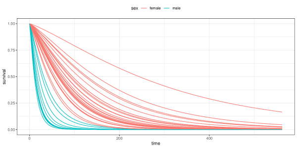
Figure 6: Posterior mean of the individual survival function from the frailty model (26).

The curves shown in Figure 6 represent the posterior mean of the probability of infection from any catheter insertion at each time considering the two replicates per patient.

Joint models of longitudinal and survival data

Joint modelling of longitudinal and time-to-event data is an increasingly productive area of statistical research that examines the association between longitudinal and survival processes (Rizopoulos, 2012). It enhances survival modelling with the inclusion of internal time-dependent covariates as well as longitudinal modelling by allowing for the inclusion of non-ignorable dropout mechanisms through survival tools. Joint models were introduced during the 90s (DeGruttola and Tu, 1994; Tsiatis et al., 1995; Faucett and Thomas, 1996; Wulfsohn and Tsiatis, 1997) and since then, have been applied to a great variety of studies mainly in epidemiological and biomedical areas.

Bayesian joint models assume a full joint distribution for the longitudinal ($y$) and the survival processes ($s$) as well as the subject-specific random effects vector ($\bm{b}$) and the parameters and hyperparameters ($\bm{\theta}$) of the model (Armero et al., 2018). Usually, they can be defined as follow:

$$f(y,s,{\bm{b}},{\bm{\theta}})=f(y,s\mid{\bm{b}},{\bm{\theta}})\,f({\bm{b}}\mid{\bm{\theta}})\,\pi({\bm{\theta}}),$$ (27)

which factorises as the product of the joint conditional distribution $f(y,s\mid{\bm{b}},{\bm{\theta}})$, the conditional distribution $f({\bm{b}}\mid{\bm{\theta}})$ of the random effects, and the prior distribution $\pi({\bm{\theta}})$. There are different proposals for the specification of the conditional distribution $f(y,s\mid{\bm{b}},{\bm{\theta}})$. The most popular approaches are the share-parameter models and the joint latent class models.

Shared-parameter models are a type of joint models where the longitudinal and time-to-event processes are connected by means of a common set of subject-specific random effects. These models make possible to quantify both the population and individual effects of the underlying longitudinal outcome on the risk of an event and allow to obtain individualised time-dynamic predictions (Wu and Carroll, 1988; Hogan and Laird, 1997, 1998). In particular, this approach postulates conditional independence between the longitudinal and survival processes given the random effects and the parameters:

$$f(y,s\mid{\bm{b}},{\bm{\theta}})=f(y\mid{\bm{b}},{\bm{\theta}})f(s\mid{\bm{b}},{\bm{\theta}}).$$

The joint latent class model is based on finite mixtures (Proust-Lima et al., 2014). Heterogeneity among the individuals is classified into a finite number $G$ of homogeneous latent clusters which share the same longitudinal trajectory and the same risk function. Both elements are also conditionally independent within the subsequent latent group as follows:

$$f(y,s\mid L=g,{\bm{b}},{\bm{\theta}})=f(y\mid L=g,{\bm{b}},{\bm{\theta}})f(s\mid L=g,{\bm{\theta}}),$$

where $L$ is a random variable that measures the uncertainty on the membership of each individual to each group, usually modelled by means of a multinomial logistic model. These models are possibly the most complex. Predicting observations from models with random effects is not easy. In this case, predicting longitudinal observations will be complicated because the conditional marginal distribution $f(y\mid L=g,{\bm{b}},{\bm{\theta}})$ necessary to obtain the corresponding predictive posterior distribution depends on both random effects and latent groups. On the other hand, the prediction of survival times does seem to be computationally simpler because the conditional distribution $f(s\mid L=g,{\bm{\theta}})$ does not depend on individual random effects.

All these proposals account for a particular type of conditional independence between the longitudinal and the survival processes which facilitates the modelling into longitudinal and survival submodels with various types of connectors. This general structure allows any type of modelling for the survival process such as frailty survival regression models, competing risks with frailties, cure models with frailties as well as linear mixed models or generalised linear mixed models for the longitudinal process (Taylor et al., 2013; Rizopoulos et al., 2015; Armero et al., 2016b; Rué et al., 2017). See Armero (2020) for a short review on Bayesian joint models up to date.

prothro dataset

We consider a liver cirrhosis dataset, referred to as prothro (longitudinal information) and prothros (survival information). It is available from the JMbayes package (Rizopoulos, 2019):

R> library("JMbayes")
R> data("prothro")
R> data("prothros")
R> str(prothro); str(prothros)
’data.frame’:Ψ2968 obs. of  9 variables:
 $ id   : num  1 1 1 2 2 2 2 2 2 2 ...
 $ pro  : num  38 31 27 51 73 90 64 54 58 90 ...
 $ time : num  0 0.244 0.381 0 0.687 ...
 $ treat: Factor w/ 2 levels "placebo","prednisone": 2 2 2 2 2 2 2 2 2 2 ...
 $ Time : num  0.413 0.413 0.413 6.754 6.754 ...
 $ start: num  0 0.244 0.381 0 0.687 ...
 $ stop : num  0.244 0.381 0.413 0.687 0.961 ...
 $ death: num  1 1 1 1 1 1 1 1 1 1 ...
 $ event: num  0 0 1 0 0 0 0 0 0 0 ...
’data.frame’:Ψ488 obs. of  4 variables:
 $ id   : num  1 2 3 4 5 6 7 8 9 10 ...
 $ Time : num  0.413 6.754 13.394 0.794 0.75 ...
 $ death: num  1 1 0 1 1 1 1 0 0 1 ...
 $ treat: Factor w/ 2 levels "placebo","prednisone": 2 2 2 2 2 2 1 1 1 1 ...

These datasets are part of a placebo-controlled randomised trial on 488 liver cirrhosis patients, where the longitudinal observations of a biomarker (prothrombin) are recorded (Andersen et al., 1993). For our illustrative purpose, only the following variables are relevant:

• id: patient number.

• pro: prothrombin measurements.

• time: time points at which the prothrombin measurements were taken.

• treat: randomised treatment (placebo or prednisone).

• Time: time (in years) from the start of treatment until death or censoring.

• death: censoring indicator (1: if patient is died; 0: otherwise).

Model implementation

We assume a shared-parameter model specified by a linear mixed-effects model (Laird and Ware, 1982) for the longitudinal response and a Cox model for the survival part. The linear mixed-effects model which describes the subject-specific prothrombin evolution of individual $i$ over time is given by:

$$y_{i}(t)=\beta_{L1}+b_{i1}+(\beta_{L2}+b_{i2})\,t+\beta_{L3}\texttt{treat}+\epsilon_{i}(t),\;\;\;i=1,\ldots,n,$$ (28)

where $y_{i}(t)$ represents the prothrombin value at time $t$ for individual $i$; $\beta_{L1}$ and $\beta_{L2}$ are fixed effects for intercept and slope, respectively, with $b_{i1}$ and $b_{i2}$ being the respective individual random effects; $\beta_{L3}$ is the regression coefficient for the treat covariate; and $\epsilon_{i}(t)$ is a measurement error for individual $i$ at time $t$. We assume that the individual random effects, ${\bm{b}_{i}}=(b_{i1},b_{i2})^{\top}$, given $\Sigma$ follow a joint bivariate normal distribution with mean vector $(0,0)^{\top}$ and variance-covariance matrix $\Sigma$, and that the errors are conditionally i.i.d. as $(\epsilon_{i}(t)\mid\sigma^{2})\sim\mbox{N}(0,\sigma^{2})$, where $\sigma^{2}$ represents the error variance. Random effects and error terms were assumed mutually independent.

Survival time for individual $i$ is modelled from a proportional hazard specification which includes in the exponential term the random effects $b_{i1}$ and $b_{i2}$ in (28) as follows:

$$h_{i}(t\mid h_{0},{\bm{\beta}}_{S},\gamma,{\bm{b}_{i}})=h_{0}(t)\exp\left\{\beta_{S2}\texttt{treat}+\gamma(b_{i1}+b_{i2}t)\right\},$$ (29)

with $h_{0}(t)=\lambda\,\alpha\,t^{\alpha-1}$ specified as a Weibull baseline hazard function, where $\alpha$ and $\lambda=\exp(\beta_{S1})$ are the shape and scale parameters, respectively; $\beta_{S2}$ is the regression coefficient for the treat covariate; and $\gamma$ is an association parameter that measure the strength of the link between the random effects associated to individual $i$ of the longitudinal submodel and their risk of death at time $t$.

We assume prior independence and specify prior marginal distributions based on non-informative distributions commonly employed in the literature. $\beta_{L}$’s, $\beta_{S}$’ and $\gamma$ follow a N($0,0.001$), while $\alpha$ and $\sigma$ follow a Un($0,10$) and a Un($0,100$), respectively, and $\Sigma$ follows an Inv-Wishart($V,r$), where $V$ is a 2$\times$2 identity matrix and $r=2$ is the degrees-of-freedom parameter. The position of the inverse-Wishart distribution in parameter space is specified by $V$, while $r$ set the certainty about the prior information in the scale matrix (Schuurman et al., 2016). The larger the $r$, the higher the certainty about the information in $V$, and the more informative is the distribution. Hence, in our application, the least informative specification then results when $r=2$ (number of random effects), which is the lowest possible number of $r$. Additionally, $V$ as an identity matrix has the appealing feature that each of the correlations in $\Sigma$ has, marginally, a uniform prior distribution (Gelman et al., 2013).

Our variable of interest is Time (prothros file), which represents the time from the start of treatment until death or censoring. The death=1 variable indicates an uncensored time:

R> # Number of patients and number of longitudinal observations per patient
R> n <- nrow(prothros)
R> M <- table(prothro$id)
R> # Survival and censoring times
R> Time <- prothros$Time
R> death <- prothros$death

The (log)prothrombin observations and their respective measurement times (prothro file) have been rearranged in matrix format:

R> # Longitudinal information in matrix format
R> time <- matrix(NA, n, max(M))
R> log.proth <- matrix(NA, n, max(M))
R> count <- 1
R> for(i in 1:n){
+     log.proth[i, 1:M[i]] <- log(prothro$pro[count:(M[i] + count - 1)])
+     time[i, 1:M[i]] <- prothro$time[count:(M[i] + count - 1)]
+     count <- count + M[i]
+  }

We have created the survival design matrix composed of an intercept and a treatment variable:

R> treat <- as.numeric(prothros$treat) - 1 # Reference = placebo
R> XS <- model.matrix(~ treat) # Fixed effects

We have split the longitudinal design matrix into two parts, XL (fixed effects) and ZL (random effects):

R> XL <- array(1, dim = c(n, max(M), 3)) # Fixed effects
R> XL[, , 2] <- time; XL[, , 3] <- treat
R> ZL <- array(1, dim = c(n, max(M), 2)) # Random effects
R> ZL[, , 2] <- time

The survival function for individual $i$, $S_{i}(t\mid h_{0},{\bm{\beta}}_{S},\gamma,{\bm{b}_{i}})=\exp\left\{-\int_{0}^{t}\,h_{i}(u\mid h_{0},{\bm{\beta}}_{S},\gamma,{\bm{b}_{i}})\,\mbox{d}u\right\}$can be efficiently approximated using some Gaussian quadrature method, available from the statmod package (Smyth et al., 2020). For our analysis, we have used 15-point Gauss-Legendre quadrature rule, as is done in Armero et al. (2018):

R> # Gauss-Legendre quadrature (15 points)
R> library("statmod")
R> glq <- gauss.quad(15, kind = "legendre")
R> xk <- glq$nodes   # Nodes
R> wk <- glq$weights # Weights
R> K <- length(xk)   # K-points

Listing 7 shows a generic implementation of a joint model in BUGS syntax using prothro/prothros data.

Listing 7: Joint model in BUGS syntax (file named as JM.txt).

⬇

1model{

2 for(i in 1:n){

3 # Longitudinal observations

4 for(j in 1:M[i]){

5 log.proth[i,j] ~ dnorm(mu[i,j],tau)

6 mu[i,j] <- inprod(betaL[],XL[i,j,]) + inprod(b[i,],ZL[i,j,])

7 }

8

9 # Survival and censoring times

10 # Hazard function at integration points

11 for(j in 1:K){

12 haz[i,j] <- alpha * pow(Time[i]/2*(xk[j]+1),alpha-1) *

13 exp(inprod(betaS[],XS[i,])+gamma*(b[i,1]+b[i,2]*(Time[i]/2*(xk[j]+1))))

14 }

15 # Log-survival function with Gauss-Legendre quadrature

16 logSurv[i] <- -Time[i]/2 * inprod(wk, haz[i,])

17

18 # Definition of the survival log-likelihood using zeros trick

19 phi[i] <- 100000 - death[i] * log(haz[i,K]) - logSurv[i]

20 zeros[i] ~ dpois(phi[i])

21

22 # Random effects

23 b[i,1:Nb] ~ dmnorm(mub[],Omega[,])

24 }

25

26 # Prior distributions

27 for(l in 1:NbetasS){ betaS[l] ~ dnorm(0.0,0.001) }

28 gamma ~ dnorm(0.0,0.001)

29 alpha ~ dunif(0,10)

30 for(l in 1:NbetasL){ betaL[l] ~ dnorm(0.0,0.001) }

31 tau <- pow(sigma,-2)

32 sigma ~ dunif(0,100)

33 Omega[1:Nb,1:Nb] ~ dwish(V[,],Nb)

34 Sigma[1:Nb,1:Nb] <- inverse(Omega[,])

35

36 # Derived quantity

37 lambda <- exp(betaS[1])

38}

Once the variables have been defined, a list with all the elements required in the model is created:

R> d.jags <- list(n = n, M = M, Time = Time, XS = XS, log.proth = log.proth, XL = XL, ZL = ZL,
+    XS = XS, death = death, mub = rep(0, 2), V = diag(1, 2), Nb = 2, zeros = rep(0, n),
+    NbetasL = dim(XL)[3], NbetasS = ncol(XS), K = length(xk), xk = xk, wk = wk)

The variables mub and V represent, respectively, the mean of the random effects normally distributed and the scale matrix of the Wishart distribution which models the precision of the random effects.

The initial values for each joint model parameter are passed to JAGS using a function that returns a list of random values:

R> i.jags <- function(){
+    list(betaS = rnorm(ncol(XS)), gamma = rnorm(1), alpha = runif(1),
+      betaL = rnorm(dim(XL)[3]), sigma = runif(1), Omega = diag(runif(2)))
+  }

The vector of monitored/saved parameters is:

R> p.jags <- c("betaS", "gamma", "alpha", "lambda", "betaL", "sigma", "Sigma", "b")

Next, the JAGS model is compiled:

R> library("rjags")
R> m7 <- jags.model(data = d.jags, file = "JM.txt", inits = i.jags, n.chains = 3)

We now run the model for 1000 burn-in simulations:

R> update(m7, 1000)

Finally, the model is run for 10000 additional simulations to keep one in 10 so that a proper thinning is done:

R> res <- coda.samples(m7, variable.names = p.jags, n.iter = 10000, thin = 10)

Similarly to the first example in Section 2.1, numerical and graphical summaries of the model parameters can be obtained using the summary and densplot functions, respectively. Gelman and Rubin’s convergence diagnostic can be calculated with the gelman.diag function, and the traceplot function provides a visual way to inspect sampling behaviour and assesses mixing across chains and convergence.

Next, simulations from the three Markov chains are merged together for inference:

R> result <- as.mcmc(do.call(rbind, res))

The posterior samples of each parameter are obtained by:

R> Sigma2.11 <- result[,1]; Sigma2.12 <- result[,2]; Sigma2.22 <- result[,4]
R> alpha <- result[,5]; b1 <- result[,6:(n+5)]; b2 <- result[,(n+6):(2*n+5)]
R> betaL1 <- result[,(2*n+6)]; betaL2 <- result[,(2*n+7)]; betaL3 <- result[,(2*n+8)]
R> betaS2 <- result[,(2*n+10)]; gamma <- result[,(2*n+11)]
R> lambda <- result[,(2*n+12)]; sigma <- result[,(2*n+13)]

Table 6 shows posterior summaries for the joint model parameters using prothro/prothros data.

Table 6: Posterior summaries for the joint model parameters.

Parameter	Mean	SD	$2.5\%$	$50\%$	$97.5\%$	$P(\cdot>0\mid\mbox{data})$
$\beta_{S2}$ (treat)	0.073	0.138	-0.191	0.071	0.343	0.703
$\gamma$ (assoc)	-2.269	0.180	-2.640	-2.264	-1.923	0.000
$\lambda$	0.187	0.023	0.145	0.186	0.233	1.000
$\alpha$	0.934	0.049	0.841	0.934	1.034	1.000
$\beta_{L1}$ (intercept)	4.276	0.021	4.235	4.276	4.318	1.000
$\beta_{L2}$ (slope)	-0.004	0.007	-0.018	-0.004	-0.010	0.301
$\beta_{L3}$ (treat)	-0.099	0.030	-0.159	-0.098	-0.040	0.000
$\sigma$	0.258	0.004	0.250	0.258	0.265	1.000
$\Sigma_{11}$	0.098	0.008	0.083	0.098	0.116	1.000
$\Sigma_{22}$	0.013	0.001	0.011	0.013	0.017	1.000
$\Sigma_{12}$	-0.003	0.003	-0.009	-0.003	0.003	0.145

Most of the parameters are interpreted similarly to the ones in previous examples. However, the association parameter, $\gamma$, plays an important role in this type of models. In our illustration, the posterior mean of $\gamma$ is negative, -2.269, and $P(\gamma>0\mid\mbox{data})=0$, indicating a strong negative association of the prothrombin measurements with respect to vital status. In other words, a negative value for $\gamma$ means that low values or decreasing trends of prothrombin increase the risk of death.

Conclusions

The analysis of time until an event of interest requires a suitable and flexible modelling and has applications in several applied fields. The BUGS language offers the opportunity of easily use and adapt Bayesian hierarchical models without the need to manually implement Markov chain Monte Carlo methods. Hence, this paper has summarised some of the most popular survival models and has focused on the Bayesian paradigm to make the inferential procedure. Furthermore, for each of the models proposed we have provided the codes in BUGS syntax, so that model can be fit with the support of the rjags package from the R language.

We have discussed all the implementation details of the following Bayesian survival models: accelerated failure time, proportional hazards, mixture cure, competing risks, multi-state, frailty, and joint models of longitudinal and survival data. Moreover, the computation of quantities of interest derived from posterior samples has been provided as well as some graphs that assist in the interpretation of results and decision making. The paper has also briefly presented other Bayesian R-packages that handle time-to-event data.

In conclusion, we hope this paper will encourage researchers who use survival models make their analyses based on the Bayesian paradigm from the BUGS codes we have provided and easily adapt them to novel settings. In addition, the descriptions of the survival models provided herein could also be used as a guidance to implement these models using other similar languages such as, for example, Stan (Carpenter et al., 2017).

Appendix A Implementation of the transition probabilities of the semi-Markov multi-state model based on posterior samples

Figure 5 was generated from the transition probabilities (16)–(21) based on posterior samples of the illness-death model parameter (22)–(24). In particular, we set a grid of time values to evaluate the transition probabilities and used the median values of age and year covariates. In this example, we are interested in the transition probabilities for patients with and without prior bypass surgery (i.e., surgery equal to 1 or 0, respectively):

R> grid <- seq(0, 1000, length.out = 51)
R> x0 <- c(median(heart2$age), median(heart2$year), 0)
R> x1 <- c(median(heart2$age), median(heart2$year), 1)

For our Weibull baseline hazard specification, the transition probability $p_{11}(s,t\mid\bm{\theta})$ (see Equation 16) can be calculated analytically and is expressed by:

$$p_{11}(s,t\mid\bm{\theta})=\exp\Big{\{}-\lambda_{1}\eta_{1}\big{[}t^{\alpha_{1}}-s^{\alpha_{1}}\big{]}-\lambda_{3}\eta_{3}\big{[}t^{\alpha_{3}}-s^{\alpha_{3}}\big{]}\Big{\}},$$ (30)

where $\eta_{k}=\exp\big{(}{\bm{x}}^{\top}{\bm{\beta}}_{k}\big{)}$, for $k=1,3$. Equation (30) is implemented as follows:

R> p11_s_t <- function(tt, ss, l1, a1, b1, l2, a2, b2, x){
+    H1 <- l1 * exp(sum(b1 * x)) * (tt^a1 - ss^a1)
+    H2 <- l2 * exp(sum(b2 * x)) * (tt^a2 - ss^a2)
+    return(exp(-H1 - H2))
+  }

Next, we have created a function mcmc_p11_s_t that takes posterior samples of each parameter from JAGS and computes $p_{11}(s,t\mid\bm{\theta})$ in (30) for a grid of time values (variable grid) using covariates x (here x0 or x1). Note that mcmc_p11_s_t is based on the mclapply function, available from the parallel package to speed computations up (R Core Team, 2020).

R> library("parallel")
R> options(mc.cores = detectCores())
R> mcmc_p11_s_t <- function(t.pred, s.pred, l1, a1, b1, l2, a2, b2, x){
+    # Sub-sample to speed up computations
+    samples.idx <- sample(1:length(l1), 200)
+    res <- sapply(t.pred, function(tt){
+      aux <- mclapply(samples.idx, function(i){
+        p11_s_t(tt, ss = s.pred, l1 = l1[i], a1 = a1[i], b1 = b1[i,],
+          l2 = l2[i], a2 = a2[i], b2 = b2[i,], x = x)
+        })
+        return(mean(unlist(aux)))
+    })
+    return(res)
+  }

As previously mentioned, we are interested in the transition probabilities for patients with and without prior bypass surgery. In particular, $p_{11}(s,t\mid\bm{\theta})$ for $s=0$ can be calculated as follows:

R> p11_0_t_surgery0 <- mcmc_p11_s_t(t.pred = grid, s.pred = 0, l1 = lambda1, a1 = alpha1,
+    b1 = cbind(beta11, beta21, beta31), l2 = lambda2, a2 = alpha2,
+    b2 = cbind(beta12, beta22, beta32), x = x0)
R> p11_0_t_surgery1 <- mcmc_p11_s_t(t.pred = grid, s.pred = 0, l1 = lambda1, a1 = alpha1,
+    b1 = cbind(beta11, beta21, beta31), l2 = lambda2, a2 = alpha2,
+    b2 = cbind(beta12, beta22, beta32), x = x1)

Finally, these transition probabilities for x0 and x1 are plotted in Figure 5 using the following code:

R> library("ggplot2")
R> surg.colour <- rep(c("no", "yes"), each = length(grid))
R> df11 <- data.frame(time = rep(grid, 2), surgery = factor(surg.colour),
+    transition = c(p11_0_t_surgery0, p11_0_t_surgery1))
R> p11 <- ggplot(data = df11, aes(x = time, y = transition, group = surgery, colour = surgery)) +
+    geom_line() + annotate("text", x = 880, y = 1, label=expression(1 %->% 1), size=5) +
+    ylab("probability") + theme(legend.position = "top") + ylim(0,1) + theme_bw()

The transition probability $p_{22}(s,t\mid\bm{\theta})$ (see Equation 17) using the Weibull baseline hazard specification is written as:

$$p_{22}(s,t\mid\bm{\theta})=\frac{\lambda_{1}\alpha_{1}\eta_{1}}{1-\exp\big{\{}-\lambda_{1}\eta_{1}s^{\alpha_{1}}\big{\}}}\int_{0}^{s}u^{\alpha_{1}-1}\exp\Big{\{}-\lambda_{1}\eta_{1}u^{\alpha_{1}}-\lambda_{3}\eta_{3}\big{[}(t-u)^{\alpha_{3}}-(s-u)^{\alpha_{3}}\big{]}\Big{\}}\,\mbox{d}u,$$ (31)

where $\eta_{k}=\exp\big{(}{\bm{x}}^{\top}{\bm{\beta}}_{k}\big{)}$, for $k=1,3$. The integral in (31) has no closed form, so some approximate method of integration is required. To do this, we first have created a function int_p22 to calculate this integral:

R> int_p22 <- function(u, tt, ss, l1, a1, b1, l3, a3, b3, x){
+    F1 <- 1 - exp(-l1 * exp(sum(b1 * x)) * ss^a1)
+    u1 <- ifelse(u > 0, u^(a1 - 1),0)
+    h1 <- l1 * a1 * exp(sum(b1 * x)) * u1
+    H1 <- l1 * exp(sum(b1 * x)) * u^a1
+    H3 <- l3 * exp(sum(b3 * x)) * ((tt - u)^a3 - (ss - u)^a3)
+    return(h1 * exp(-H1 - H3) / F1)
+  }

Next, we have created a function p22_s_t that computes $p_{22}(s,t\mid\bm{\theta})$ in (31) by integrating out the int_p22 function using the integral function available from the pracma package (Borchers, 2019).

R> library("pracma")
R> p22_s_t <- function(tt, ss, l1, a1, b1, l3, a3, b3, x){
+    return(integral(int_p22, xmin = 0, xmax = ss, method = "Kronrod", tt = tt,
+      ss = ss, l1 = l1, a1 = a1, b1 = b1, l3 = l3, a3 = a3, b3 = b3, x = x))
+  }

Analogous to the previous case, we have created a function mcmc_p22_s_t that takes posterior samples of each parameter from JAGS and computes $p_{22}(s,t\mid\bm{\theta})$ in (31) for a grid of time values (variable grid) using covariates x (here x0 or x1).

R> mcmc_p22_s_t <- function(t.pred, s.pred, l1, a1, b1, l3, a3, b3, x){
+    # Sub-sample to speed up computations
+    samples.idx <- sample(1:length(l1), 200)
+    res <- sapply(t.pred, function(tt){
+      aux <- mclapply(samples.idx, function(i){
+        p22_s_t(tt, ss = s.pred, l1 = l1[i], a1 = a1[i], b1 = b1[i,],
+          l3 = l3[i], a3 = a3[i], b3 = b3[i,], x = x)
+      })
+      return(mean(unlist(aux)))
+    })
+    return(res)
+  }

Note that the transition time from state 1 to state 2 prevents the case $s=0$ in $p_{22}(s,t\mid\bm{\theta})$. To realistically get around this problem, we have set $s$ as the median time of patients who transitioned from state 1 to 2 ($s=26$) and add this amount to the grid of time values. So, we have calculated the transition probabilities (31) for x0 and x1:

R> m <- median(heart2$times1[heart2$delta == 1])
R> grid2 <- grid + m
R> p22_m_t_surgery0 <- mcmc_p22_s_t(t.pred = grid2, s.pred = m, l1 = lambda1, a1 = alpha1,
+    b1 = cbind(beta11, beta21, beta31), l3 = lambda3, a3 = alpha3,
+    b3 = cbind(beta13, beta23, beta33), x = x0)
R> p22_m_t_surgery1 <- mcmc_p22_s_t(t.pred = grid2, s.pred = m, l1 = lambda1, a1 = alpha1,
+    b1 = cbind(beta11, beta21, beta31), l3 = lambda3, a3 = alpha3,
+    b3 = cbind(beta13, beta23, beta33), x = x1)

Finally, these transition probabilities are plotted in Figure 5 using the following code:

R> df22 <- data.frame(time = rep(grid, 2), surgery = factor(surg.colour),
+    transition = c(p22_m_t_surgery0, p22_m_t_surgery1))
R> p22 <- ggplot(data = df22, aes(x = time, y = transition, group = surgery, colour = surgery)) +
+    geom_line() + annotate("text", x = 880, y = 1, label=expression(2 %->% 2), size=5) +
+    ylab("probability") + theme(legend.position = "top") + ylim(0,1) + theme_bw()

The transition probability $p_{12}(s,t\mid\bm{\theta})$ (see Equation 18) using the Weibull baseline hazard specification is written as:

$$p_{12}(s,t\mid\bm{\theta})=\lambda_{1}\alpha_{1}\eta_{1}\int_{s}^{t}u^{\alpha_{1}-1}\exp\Big{\{}-\lambda_{1}\eta_{1}\big{[}u^{\alpha_{1}}-s^{\alpha_{1}}\big{]}-\lambda_{2}\eta_{2}\big{[}u^{\alpha_{2}}-s^{\alpha_{2}}\big{]}-\lambda_{3}\eta_{3}(t-u)^{\alpha_{3}}\Big{\}}\,\mbox{d}u,$$ (32)

where $\eta_{k}=\exp\big{(}{\bm{x}}^{\top}{\bm{\beta}}_{k}\big{)}$, for $k=1,2,3$. Analogous to the previous case, the integral in (32) has no closed form, so some approximate method of integration is required. To do this, we first have created a function int_p12 to calculate this integral:

R> int_p12 <- function(u, tt, ss, l1, a1, b1, l2, a2, b2, l3, a3, b3, x){
+    u1 <- ifelse(u > 0, u^(a1 - 1), 0)
+    h1 <- l1 * a1 * exp(sum(b1 * x)) * u1
+    H1 <- l1 * exp(sum(b1 * x)) * (u^a1 - ss^a1)
+    H2 <- l2 * exp(sum(b2 * x)) * (u^a2 - ss^a2)
+    H3 <- l3 * exp(sum(b3 * x)) * (tt - u)^a3
+    return(h1 * exp(-H1 - H2 - H3))
+  }

Next, we have created a function p12_s_t that computes $p_{12}(s,t\mid\bm{\theta})$ in (32) by integrating out the int_p12 function.

R> p12_s_t <- function(tt, ss, l1, a1, b1, l2, a2, b2, l3, a3, b3, x){
+    return(integral(int_p12, xmin = ss, xmax = tt, method = "Kronrod", tt = tt,
+      ss = ss, l1 = l1, a1 = a1, b1 = b1, l2 = l2, a2 = a2, b2 = b2,
+      l3 = l3, a3 = a3, b3 = b3, x = x))
+  }

As a last step, we have created a function mcmc_p12_s_t that takes posterior samples of each parameter from JAGS and computes $p_{12}(s,t\mid\bm{\theta})$ in (32) for a grid of time values (variable grid) using covariates x (here x0 or x1).

R> mcmc_p12_s_t <- function(t.pred, s.pred, l1, a1, b1, l2, a2, b2, l3, a3, b3, x){
+    # Sub-sample to speed up computations
+    samples.idx <- sample(1:length(l1), 200)
+    res <- sapply(t.pred, function(tt){
+      aux <- mclapply(samples.idx, function(i){
+        p12_s_t(tt, ss = s.pred, l1 = l1[i], a1 = a1[i], b1 = b1[i,], l2 = l2[i],
+          a2 = a2[i], b2 = b2[i,], l3 = l3[i], a3 = a3[i], b3 = b3[i,], x = x)
+      })
+      return(mean(unlist(aux)))
+    })
+    return(res)
+  }

The transition probabilities $p_{12}(s,t\mid\bm{\theta})$ of x0 and x1 for $s=0$ can be calculated as follows:

R> p12_0_t_surgery0 <- mcmc_p12_s_t(t.pred = grid, s.pred = 0, l1 = lambda1, a1 = alpha1,
+    b1 = cbind(beta11, beta21, beta31), l2 = lambda2, a2 = alpha2,
+    b2 = cbind(beta12, beta22, beta32), l3 = lambda3, a3 = alpha3,
+    b3 = cbind(beta13, beta23, beta33), x = x0)
R> p12_0_t_surgery1 <- mcmc_p12_s_t(t.pred = grid, s.pred = 0, l1 = lambda1, a1 = alpha1,
+    b1 = cbind(beta11, beta21, beta31), l2 = lambda2, a2 = alpha2,
+    b2 = cbind(beta12, beta22, beta32), l3 = lambda3, a3 = alpha3,
+    b3 = cbind(beta13, beta23, beta33), x = x1)

Finally, these transition probabilities are plotted in Figure 5 using the following code:

R> df12 <- data.frame(time = rep(grid, 2), surgery = factor(surg.colour),
+    transition = c(p12_0_t_surgery0, p12_0_t_surgery1))
R> p12 <- ggplot(data = df12, aes(x = time, y = transition, group = surgery, colour = surgery)) +
+    geom_line() + annotate("text", x = 880, y = 1, label=expression(1 %->% 2), size=5) +
+    ylab("probability") + theme(legend.position = "top") + ylim(0,1) + theme_bw()

As shown in (19) and (20), $p_{13}(s,t\mid\bm{\theta})$ and $p_{23}(s,t\mid\bm{\theta})$ are derived from the previously calculated transition probabilities. So, we can get them for x0 and x1 as follows:

R> p13_0_t_surgery0 <- 1 - p11_0_t_surgery0 - p12_0_t_surgery0
R> p13_0_t_surgery1 <- 1 - p11_0_t_surgery1 - p12_0_t_surgery1
R> p23_m_t_surgery0 <- 1 - p22_m_t_surgery0
R> p23_m_t_surgery1 <- 1 - p22_m_t_surgery1

These transition probabilities are plotted in Figure 5 using the following code:

R> df13 <- data.frame(time = rep(grid, 2), surgery = factor(surg.colour),
+    transition = c(p13_0_t_surgery0, p13_0_t_surgery1))
R> df23 <- data.frame(time = rep(grid, 2), surgery = factor(surg.colour),
+    transition = c(p23_m_t_surgery0, p23_m_t_surgery1))
R> p13 <- ggplot(data = df13, aes(x = time, y = transition, group = surgery, colour = surgery)) +
+    geom_line() + annotate("text", x = 880, y = 1, label=expression(1 %->% 3), size=5) +
+    ylab("probability") + theme(legend.position = "top") + ylim(0,1) + theme_bw()
R> p23 <- ggplot(data = df23, aes(x = time, y = transition, group = surgery, colour = surgery)) +
+    geom_line() + annotate("text", x = 880, y = 1, label=expression(2 %->% 3), size=5) +
+    ylab("probability") + theme(legend.position = "top") + ylim(0,1) + theme_bw()

To show these graphs in two rows and three columns, as in Figure 5, we have used the grid.arrange function available from the gridExtra package (Auguie and Antonov, 2017).

R> library("gridExtra")
R> grid.arrange(p11, p12, p13, p22, p23, nrow = 2, ncol = 3,
+    layout_matrix = rbind(c(1, 2, 3), c(NA, 5, 6)))

References

- Aalen (1994) O. O. Aalen. Effects of Frailty in Survival Analysis. Statistical Methods in Medical Research, 3(3):227–243, 1994. doi: 10.1177/096228029400300303.
- Alvares et al. (2019) D. Alvares, S. Haneuse, C. Lee, and K. H. Lee. SemiCompRisks: An R Package for the Analysis of Independent and Cluster-correlated Semi-competing Risks Data. The R Journal, 11(1):376–400, 2019. doi: 10.32614/rj-2019-038.
- Andersen and Keiding (2002) P. K. Andersen and N. Keiding. Multi-state Models for Event History Analysis. Statistical Methods in Medical Research, 11(2):91–115, 2002. doi: 10.1191/0962280202sm276ra.
- Andersen and Perme (2008) P. K. Andersen and M. P. Perme. Inference for Outcome Probabilities in Multi-state Models. Lifetime Data Analysis, 14(4):405–431, 2008. doi: 10.1007/s10985-008-9097-x.
- Andersen et al. (1993) P. K. Andersen, Ø. Borgan, R. D. Gill, and N. Keiding. Statistical Models Based on Counting Processes. Springer, 1st edition, 1993.
- Armero (2020) C. Armero. Bayesian Joint Models for Longitudinal and Survival Data. Wiley StatsRef: Statistics Reference Online, 2020. doi: arXiv:2005.12822.
- Armero et al. (2016a) C. Armero, S. Cabras, M. E. Castellanos, S. Perra, A. Quirós, M. J. Oruezábal, and J. Sánchez-Rubio. Bayesian Analysis of a Disability Model for Lung Cancer Survival. Statistics Methods in Medical Research, 25(1):336–351, 2016a. doi: 10.1177/0962280212452803.
- Armero et al. (2016b) C. Armero, C. Forné, M. Rué, A. Forte, H. Perpiñán, G. Gómez, and M. Baré. Bayesian Joint Ordinal and Survival Modeling for Breast Cancer Risk Assessment. Statistics in Medicine, 35(28):5267–5282, 2016b. doi: 10.1002/sim.7065.
- Armero et al. (2018) C. Armero, A. Forte, H. Perpiñán, M. J. Sanahuja, and S. Agustí. Bayesian Joint Modeling for Assessing the Progression of Chronic Kidney Disease in Children. Statistical Methods in Medical Research, 27(1):298–311, 2018. doi: 10.1177/0962280216628560.
- Auguie and Antonov (2017) B. Auguie and A. Antonov. gridExtra: Miscellaneous Functions for “Grid” Graphics. R package version 2.3, https://CRAN.R-project.org/package=gridExtra, 2017.
- Berkson and Gage (1952) J. Berkson and R. P. Gage. Survival Curve for Cancer Patients Following Treatment. Journal of the American Statistical Association, 47(259):501–515, 1952. doi: 10.1080/01621459.1952.10501187.
- Beyersmann et al. (2007) J. Beyersmann, M. Dettenkofer, H. Bertz, and M. Schumacher. A Competing Risks Analysis of Bloodstream Infection After Stem-Cell Transplantation Using Subdistribution Hazards and Cause-Specific Hazards. Statistics in Medicine, 26(30):5360–5369, 2007. doi: 10.1002/sim.3006.
- Bogaerts et al. (2017) K. Bogaerts, A. Komárek, and E. Lesaffre. Survival Analysis with Interval-Censored Data: A Practical Approach with Examples in R, SAS, and BUGS. Chapman & Hall/CRC, 1st edition, 2017.
- Borchers (2019) H. W. Borchers. pracma: Practical Numerical Math Functions. R package version 2.2.5, https://CRAN.R-project.org/package=pracma, 2019.
- Breslow (1974) N. Breslow. Covariance Analysis of Censored Survival Data. Biometrics, 30(1):89–99, 1974. doi: 10.2307/2529620.
- Brooks and Gelman (1998) S. P. Brooks and A. Gelman. General Methods for Monitoring Convergence of Iterative Simulations. Journal of Computational and Graphical Statistics, 7(4):434–455, 1998. doi: 10.1080/10618600.1998.10474787.
- Cai et al. (2012) C. Cai, Y. Zou, Y. Peng, and J. Zhang. smcure: Fit Semiparametric Mixture Cure Models. R package version 2.0, https://CRAN.R-project.org/package=smcure, 2012.
- Carpenter et al. (2017) B. Carpenter, A. Gelman, M. Hoffman, D. Lee, B. Goodrich, M. Betancourt, M. Brubaker, J. Guo, P. Li, and A. Riddell. Stan: A Probabilistic Programming Language. Journal of Statistical Software, 76(1):1–32, 2017. doi: 10.18637/jss.v076.i01.
- Christensen et al. (2011) R. Christensen, J. Wesley, A. Branscum, and T. E. Hanson. Bayesian Ideas and Data Analysis: An Introduction for Scientists and Statisticians. Chapman & Hall/CRC, 1st edition, 2011.
- Clayton (1978) D. G. Clayton. A Model for Association in Bivariate Life Tables and Its Application in Epidemiological Studies of Familial Tendency in Chronic Disease Incidence. Biometrika, 65(1):141–151, 1978. doi: 10.1093/biomet/65.1.141.
- Collett (2015) D. Collett. Modelling Survival Data in Medical Research. Chapman & Hall/CRC, 3rd edition, 2015.
- Cox (1972) D. R. Cox. Regression Models and Life-Tables. Journal of the Royal Statistical Society. Series B (Methodological), 34(2):187–220, 1972. doi: 10.1111/j.2517-6161.1972.tb00899.x.
- Crowley and Hu (1977) J. Crowley and M. Hu. Covariance Analysis of Heart Transplant Survival Data. Journal of the American Statistical Association, 72(357):27–36, 1977. doi: 10.1080/01621459.1977.10479903.
- DeGruttola and Tu (1994) V. DeGruttola and X. M. Tu. Modelling Progression of CD4-Lymphocyte Count and Its Relationship to Survival Time. Biometrics, 50(4):1003–1014, 1994. doi: 10.2307/2533439.
- Dettenkofer et al. (2005) M. Dettenkofer, S. Wenzler-Rottele, R. Babikir, H. Bertz, W. Ebner, E. Meyer, H. Ruden, P. Gastmeier, and F. D. Daschner. Surveillance of Nosocomial Sepsis and Pneumonia in Patients with a Bone Marrow or Peripheral Blood Stem Cell Transplant: A Multicenter Project. Clinical Infectious Diseases, 40(7):926–931, 2005. doi: 10.1086/428046.
- Faucett and Thomas (1996) C. L. Faucett and D. C. Thomas. Simultaneously Modelling Censored Survival Data and Repeatedly Measured Covariates: A Gibbs Sampling Approach. Statistics in Medicine, 15(15):1663–1685, 1996. doi: 10.1002/(sici)1097-0258(19960815)15:15¡1663::aid-sim294¿3.0.co;2-1.
- Ge and Chen (2012) M. Ge and M. H. Chen. Bayesian Inference of the Fully Specified Subdistribution Model for Survival Data with Competing Risks. Lifetime Data Analysis, 18(3):339–363, 2012. doi: 10.1007/s10985-012-9221-9.
- Gelman and Rubin (1992) A. Gelman and D. B. Rubin. Inference from Iterative Simulation using Multiple Sequences. Statistical Science, 7(4):457–472, 1992. doi: 10.1214/ss/1177011136.
- Gelman et al. (2013) A. Gelman, J. B. Carlin, H. S. Stern, D. B. Dunson, A. Vehtari, and D. B. Rubin. Bayesian Data Analysis. Chapman & Hall/CRC, 3rd edition, 2013.
- Gilks et al. (1994) W. R. Gilks, A. Thomas, and D. J. Spiegelhalter. A Language and Program for Complex Bayesian Modelling. The Statistician, 43(1):169–177, 1994. doi: 10.2307/2348941.
- Grambauer and Neudecker (2011) N. Grambauer and A. Neudecker. compeir: Event-Specific Incidence Rates for Competing Risks Data. R package version 1.0, https://CRAN.R-project.org/package=compeir, 2011.
- Ha et al. (2018) I. D. Ha, M. Noh, J. Kim, and Y. Lee. frailtyHL: Frailty Models via Hierarchical Likelihood. R package version 2.2, https://CRAN.R-project.org/package=frailtyHL, 2018.
- Han et al. (2014) B. Han, M. Yu, J. J. Dignamc, and P. J. Rathouzb. Bayesian Approach for Flexible Modeling of Semicompeting Risks Data. Statistics in Medicine, 33(29):5111–5125, 2014. doi: 10.1002/sim.6313.
- Hogan and Laird (1997) J. W. Hogan and N. M. Laird. Mixture Models for the Joint Distribution of Repeated Measures and Event Times. Statistics in Medicine, 16(3):239–257, 1997. doi: 10.1002/(sici)1097-0258(19970215)16:3¡239::aid-sim483¿3.0.co;2-x.
- Hogan and Laird (1998) J. W. Hogan and N. M. Laird. Increasing Efficiency from Censored Survival Data by using Random Effects to Model Longitudinal Covariates. Statistical Methods in Medical Research, 7(1):28–48, 1998. doi: 10.1177/096228029800700104.
- Hougaard (2000) P. Hougaard. Analysis of Multivariate Survival Data. Springer, 1st edition, 2000.
- Ibrahim et al. (2001) J. G. Ibrahim, M. H. Chen, and D. Sinha. Bayesian Survival Analysis. Springer, 1st edition, 2001.
- Jara et al. (2018) A. Jara, T. Hanson, F. Quintana, P. Mueller, and G. Rosner. DPpackage: Bayesian Nonparametric Modeling in R. R package version 1.1-7.4, https://CRAN.R-project.org/package=DPpackage, 2018.
- Kalbfleisch and Prentice (2002) J. D. Kalbfleisch and R. L. Prentice. The Statistical Analysis of Failure Time Data. John Wiley & Sons, 2nd edition, 2002.
- Kardaun (1983) O. Kardaun. Statistical Survival Analysis of Male Larynx-Cancer Patients - A Case Study. Statistica Neerlandica, 37(3):103–125, 1983. doi: 10.1111/j.1467-9574.1983.tb00806.x.
- Kersey et al. (1987) J. H. Kersey, D. Weisdorf, M. E. Nesbit, T. W. LeBien, W. G. Woods, P. B. McGlave, T. Kim, D. A. Vallera, A. I. Goldman, B. Bostrom, D. Hurd, and N. K. C. Ramsay. Comparison of Autologous and Allogeneic Bone Marrow Transplantation for Treatment of High-Risk Refractory Acute Lymphoblastic Leukemia. New England Journal of Medicine, 317(8):461–467, 1987. doi: 10.1056/nejm198708203170801.
- Klein and Moeschberger (2003) J. P. Klein and M. L. Moeschberger. Survival Analysis: Techniques for Censored and Truncated Data. Springer, 2nd edition, 2003.
- Klein et al. (2012) J. P. Klein, M. L. Moeschberger, and J. Yan. KMsurv: Data Sets from Klein and Moeschberger (1997), Survival Analysis. R package version 0.1-5, https://CRAN.R-project.org/package=KMsurv, 2012.
- Klein et al. (2013) J. P. Klein, H. C. van Houwelingen, J. G. Ibrahim, and T. H. Scheike. Handbook of Survival Analysis. Chapman & Hall/CRC, 1st edition, 2013.
- Kleinbaum and Klein (2012) D. G. Kleinbaum and M. Klein. Survival Analysis: A Self-Learning Text. Springer, 3rd edition, 2012.
- Komárek (2018) A. Komárek. bayesSurv: Bayesian Survival Regression with Flexible Error and Random Effects Distributions. R package version 3.2, https://CRAN.R-project.org/package=bayesSurv, 2018.
- Laird and Ware (1982) N. M. Laird and J. H. Ware. Random-Effects Models for Longitudinal Data. Biometrics, 38(4):963–974, 1982. doi: 10.2307/2529876.
- Lázaro et al. (2020) E. Lázaro, C. Armero, and D. Alvares. Bayesian Regularization for Flexible Baseline Hazard Functions in Cox Survival Models. Submitted, 0(0):0–0, 2020.
- Lee et al. (2016) K. H. Lee, F. Dominici, D. Schrag, and S. Haneuse. Hierarchical Models for Semicompeting Risks Data with Application to Quality of End-of-life Care for Pancreatic Cancer. Journal of the American Statistical Association, 111(515):1075–1095, 2016. doi: 10.1080/01621459.2016.1164052.
- Lee et al. (2019) K. H. Lee, C. Lee, D. Alvares, and S. Haneuse. SemiCompRisks: Hierarchical Models for Parametric and Semi-Parametric Analyses of Semi-Competing Risks Data. R package version 3.2, https://CRAN.R-project.org/package=SemiCompRisks, 2019.
- Lin et al. (2015) X. Lin, B. Cai, L. Wang, and Z. Zhang. A Bayesian Proportional Hazards Model for General Interval-Censored Data. Lifetime Data Analysis, 21(3):470–490, 2015. doi: 10.1007/s10985-014-9305-9.
- Lunn et al. (2012) D. Lunn, C. Jackson, N. Best, A. Thomas, and D. Spiegelhalter. The BUGS Book: A Practical Introduction to Bayesian Analysis. Chapman & Hall/CRC, 1st edition, 2012.
- McGilchrist and Aisbett (1991) C. A. McGilchrist and C. W. Aisbett. Regression with Frailty in Survival Analysis. Biometrics, 47(2):461–466, 1991. doi: 10.2307/2532138.
- Meira-Machado and Roca-Pardinas (2012) L. Meira-Machado and J. Roca-Pardinas. p3state.msm: Analyzing Survival Data From Illness-Death Model. R package version 1.3, https://CRAN.R-project.org/package=p3state.msm, 2012.
- Mitra and Müller (2015) R. Mitra and P. Müller, editors. Nonparametric Bayesian Inference in Biostatistics. Springer, 1st edition, 2015.
- Murray et al. (2016) T. A. Murray, B. P. Hobbs, D. J. Sargent, and B. P. Carlin. Flexible Bayesian Survival Modeling with Semiparametric Time-dependent and Shape-restricted Covariate Effects. Bayesian Analysis, 11(2):381–402, 2016. doi: 10.1214/15-BA954.
- Ntzoufras (2009) I. Ntzoufras. Bayesian Modeling using WinBUGS. John Wiley & Sons, 1st edition, 2009.
- Pan et al. (2017) C. Pan, B. Cai, L. Wang, and X. Lin. ICBayes: Bayesian Semiparametric Models for Interval-Censored Data. R package version 1.1, https://CRAN.R-project.org/package=ICBayes, 2017.
- Plummer (2003) M. Plummer. JAGS: A Program for Analysis of Bayesian Graphical Models using Gibbs Sampling. pages 1–10. Proceedings of the 3rd International Workshop on Distributed Statistical Computing, Vienna, Austria, 2003.
- Plummer (2018) M. Plummer. rjags: Bayesian Graphical Models Using MCMC. R package version 4-8, https://CRAN.R-project.org/package=rjags, 2018.
- Plummer et al. (2019) M. Plummer, N. Best, K. Cowles, K. Vines, D. Sarkar, D. Bates, R. Almond, and A. Magnusson. coda: Output Analysis and Diagnostics for MCMC. R package version 0.19-3, https://CRAN.R-project.org/package=coda, 2019.
- Proust-Lima et al. (2014) C. Proust-Lima, M. Séne, J. M. G. Taylor, and H. Jacqmin-Gadda. Joint Latent Class Models for Longitudinal and Time-To-Event Data: A Review. Statistical Methods in Medical Research, 23(1):74–90, 2014. doi: 10.1177/0962280212445839.
- Putter et al. (2007) H. Putter, M. Fiocco, and R. B. Geskus. Tutorial in Biostatistics: Competing Risks and Multi-State Models. Statistics in Medicine, 26(11):2389–2430, 2007. doi: 10.1002/sim.2712.
- R Core Team (2020) R Core Team. R: A Language and Environment for Statistical Computing. R Foundation for Statistical Computing, https://www.R-project.org, 2020.
- Raftery et al. (2018) A. Raftery, J. Hoeting, C. Volinsky, I. Painter, and K. Y. Yeung. BMA: Bayesian Model Averaging. R package version 3.18.9, https://CRAN.R-project.org/package=BMA, 2018.
- Rizopoulos (2012) D. Rizopoulos. Joint Models for Longitudinal and Time-To-Event Data: With Applications in R. Chapman & Hall/CRC, 1st edition, 2012.
- Rizopoulos (2019) D. Rizopoulos. JMbayes: Joint Modeling of Longitudinal and Time-to-Event Data Under a Bayesian Approach. R package version 0.8-83, https://CRAN.R-project.org/package=JMbayes, 2019.
- Rizopoulos et al. (2015) D. Rizopoulos, J. M. G. Taylor, J. V. Rosmalen, E. W. Steyerberg, and J. J. M. Takkenberg. Personalized Screening Intervals for Biomarkers using Joint Models for Longitudinal and Survival Data. Biostatistics, 17(1):149–164, 2015. doi: 10.1093/biostatistics/kxv031.
- Royston (2011) P. Royston. Estimating a Smooth Baseline Hazard Function for the Cox Model. Research report 314, MRC Clinical Trials Unit and University College London, London, 2011.
- Rue et al. (2009) H. Rue, S. Martino, and N. Chopin. Approximate Bayesian Inference for Latent Gaussian Models Using Integrated Nested Laplace Approximations. Journal of the Royal Statistical Society. Series B (Methodological), 71(2):319–392, 2009. doi: 10.1111/j.1467-9868.2008.00700.x.
- Rué et al. (2017) M. Rué, E. R. Andrinopoulou, D. Alvares, C. Armero, A. Forte, and L. Blanch. Bayesian Joint Modeling of Bivariate Longitudinal and Competing Risks Data: An Application to Study Patient-Ventilator Asynchronies in Critical Care Patients. Biometrical Journal, 59(6):1184–1203, 2017. doi: 10.1002/bimj.201600221.
- Sahu et al. (1997) S. K. Sahu, D. K. Dey, H. Aslanidou, and D. Sinha. A Weibull Regression Model with Gamma Frailties for Multivariate Survival Data. Lifetime Data Analysis, 3(2):123–137, 1997. doi: 10.1023/a:1009605117713.
- Schuurman et al. (2016) N. K. Schuurman, R. P. P. P. Grasman, and E. L. Hamaker. A Comparison of Inverse-Wishart Prior Specifications for Covariance Matrices in Multilevel Autoregressive Models. Multivariate Behavioral Research, 51(2-3):185–206, 2016. doi: 10.1080/00273171.2015.1065398.
- Sharabiani and Mahani (2019) M. T. A. Sharabiani and A. S. Mahani. CFC: Cause-Specific Framework for Competing-Risk Analysis. R package version 1.1.2, https://CRAN.R-project.org/package=CFC, 2019.
- Smyth et al. (2020) G. Smyth, Y. Hu, P. Dunn, B. Phipson, and Y. Chen. statmod: Statistical Modeling. R package version 1.4.34, https://CRAN.R-project.org/package=statmod, 2020.
- Stan Development Team (2020) Stan Development Team. RStan: the R Interface to Stan. Stan, http://mc-stan.org/, 2020.
- Taylor et al. (2018) B. M. Taylor, B. S. Rowlingson, and Z. Zheng. spatsurv: Bayesian Spatial Survival Analysis with Parametric Proportional Hazards Models. R package version 1.2, https://CRAN.R-project.org/package=spatsurv, 2018.
- Taylor et al. (2013) J. M. G. Taylor, Y. Park, D. P. Ankerst, C. Proust-Lima, S. Williams, L. Kestin, K. Bae, T. Pickles, and H. Sandler. Real-Time Individual Predictions of Prostate Cancer Recurrence using Joint Models. Biometrics, 69(1):206–213, 2013. doi: 10.1111/j.1541-0420.2012.01823.x.
- Tsiatis et al. (1995) A. A. Tsiatis, V. DeGruttola, and M. S. Wulfsohn. Modeling the Relationship of Survival to Longitudinal Data Measured with Error. Applications to Survival and CD4 Counts in Patients with AIDS. Journal of the American Statistical Association, 90(429):27–37, 1995. doi: 10.1080/01621459.1995.10476485.
- Umlauf et al. (2019) N. Umlauf, T. Kneib, and N. Klein. BayesX: R Utilities Accompanying the Software Package BayesX. R package version 0.3-1, https://CRAN.R-project.org/package=BayesX, 2019.
- Vaupel et al. (1979) J. W. Vaupel, K. G. Manton, and E. Stallard. The Impact of Heterogeneity in Individual Frailty on the Dynamics of Mortality. Demography, 16(3):439–454, 1979. doi: 10.2307/2061224.
- Wang et al. (2017) X. Wang, M. H. Chen, W. Wang, and J. Yan. dynsurv: Dynamic Models for Survival Data. R package version 0.3-6, https://CRAN.R-project.org/package=dynsurv, 2017.
- Wu and Carroll (1988) M. C. Wu and R. J. Carroll. Estimation and Comparison of Changes in the Presence of Informative Right Censoring by Modeling the Censoring Process. Biometrics, 44(1):175–188, 1988. doi: 10.2307/2531905.
- Wulfsohn and Tsiatis (1997) M. S. Wulfsohn and A. A. Tsiatis. A Joint Model for Survival and Longitudinal Data Measured with Error. Biometrics, 53(1):330–339, 1997. doi: 10.2307/2533118.
- Zhou and Hanson (2018) H. Zhou and T. Hanson. spBayesSurv: Bayesian Modeling and Analysis of Spatially Correlated Survival Data. R package version 1.1.3, https://CRAN.R-project.org/package=spBayesSurv, 2018.