Moment Conditions for Dynamic Panel Logit Models
with Fixed Effects

Abstract

This paper investigates the construction of moment conditions in discrete choice panel data with individual specific fixed effects. We describe how to systematically explore the existence of moment conditions that do not depend on the fixed effects, and we demonstrate how to construct them when they exist. Our approach is closely related to the numerical “functional differencing” construction in Bonhomme (2012), but our emphasis is to find explicit analytic expressions for the moment functions. We first explain the construction and give examples of such moment conditions in various models. Then, we focus on the dynamic binary choice logit model and explore the implications of the moment conditions for identification and estimation of the model parameters that are common to all individuals.

1 Introduction

This paper is concerned with estimation of the common parameters in nonlinear panel data models with individual-specific fixed effects in situations where the relevant asymptotics is an increasing number of cross-sectional units observed over a fixed number of time periods. Our contribution is a general approach for constructing conditional moment conditions when the dependent variable can take a finite number of values, and we demonstrate how the approach can be used to construct moment conditions for logit models with strictly exogenous explanatory variables as well as lagged dependent variables.

The economic motivation for the econometric model investigated in this paper is the question of whether persistence in economic data is due to unobserved heterogeneity or state dependence. This question dates back to Heckman (1978) and can be formulated as a distinction between individual-specific fixed effects and lagged dependent variables. This framework has proven relevant in many areas of economics. For example, Pakes, Porter, Shepard, and Calder-Wang (2022) have employed it to study the importance of switching costs in a model of health insurance plan choice.

Econometrically, this paper makes a contribution to the literature on the estimation of nonlinear econometric models with fixed effects. The challenge is that if the fixed effects enter in a way that is not additive or multiplicative, then one cannot simply difference or quasi-difference it away as one would in a linear or multiplicative model. At the same time, treating the fixed effects as parameters to be estimated in a nonlinear model will generally lead to an inconsistent estimator of the common parameters as the number of cross-sectional units increases with the number of time periods fixed. This is what is known as the incidental parameters problem. See Neyman and Scott (1948). One solution to the incidental parameters problem in parametric models is to look for sufficient statistics for the fixed effects. By definition, the conditional likelihood, conditional on these sufficient statistics, will not depend on the fixed effects, so it can potentially be used for estimation. This approach was pioneered by Rasch (1960b) and Andersen (1970). Unfortunately, there are relatively few models for which one can find such sufficient statistics, so an alternative approach is to try to construct moment conditions that depend on the parameters of interest, but not on the individual-specific fixed effects. Papers by Honoré (1992, 1993), Hu (2002), and Johnson (2004) are earlier specific examples of this, and Bonhomme (2012) developed a general approach for obtaining moment conditions via “functional differencing.”

Our paper operationalizes the proposal in Bonhomme (2012) for the case of dependent variables with a finite number of possible values. Specifically, we offer a systematic method for how to first numerically explore the potential for constructing moment conditions and then derive their analytic expressions. We then apply this machinery to create moment conditions for a prominent case: the fixed effects logit model with strictly exogenous explanatory variables and lagged dependent variables. For models with one lag, we give explicit expressions for all available moment conditions when $T\geq 3$, where $T$ is the number of time periods in addition to those that give the initial conditions for the dependent variable. We also provide all the moment conditions for the case with two lagged dependent variables and $T=4$ and $5$, as well as with three lags and $T=5$. Notably, for the case of one lag and three time periods (in addition to the one that delivers the initial), our conditions align with those previously found by Kitazawa (2013, 2016).

Estimation of panel data binary response models dates back to Rasch (1960b), who noted that in a logit model with strictly exogenous explanatory variables, one can make inference regarding the remaining parameters by conditioning on the sums of the dependent variable for each individual. Chamberlain (1985) and Magnac (2000) demonstrated that it is also possible to find sufficient statistics for the individual-specific fixed effects in logit models where the only explanatory variables are lagged outcomes, and the common parameters can then be estimated by maximizing the conditional likelihood (conditional on the sufficient statistic). Unfortunately, the conditional likelihood approach referenced above does not generally carry over to logit models that have both lagged dependent variables and strictly exogenous explanatory variables. However, as shown in Honoré and Kyriazidou (2000), this approach does apply if one is also willing to condition on the vector of covariates being equal across certain time periods. This leads to an estimator that is asymptotically normal under suitable regularity conditions, but the rate of convergence is slower than the usual $\sqrt{n}$ when there are continuous covariates. The logit assumption is crucial in the construction of the sufficient statistics above. A number of papers (including Manski 1987, Aristodemou 2018 and Khan, Ponomareva, and Tamer 2019) have relaxed the logistic assumption. This literature suggests that point estimation is sometimes possible without the logit assumption, and that informative bounds can be constructed when it is not. On the other hand, Chamberlain (2010) showed that in a two-period static threshold-crossing model regular root-$n$ consistent estimation is only possible in a logit setting. This underpins the focus on the logistic assumption throughout this paper.

The paper is organized as follows: Section 2 details our approach for discerning and constructing moment conditions when the dependent variable assumes a finite number of values, also drawing on insights from Dobronyi, Gu, and Kim (2021) regarding the number of available moments. In Section 3, we showcase this within a panel data logit AR(1) model with $T=3$ time periods. Section 4 extends this by exploring various other models, including notably the dynamic ordered logit and dynamic multinomial models. This section also highlights the versatility of our method through examples like the panel data logit AR(1) with a heterogeneous time trend, and a static binary response model leveraging a mixture of logits. Section 5 discusses conditions under which the moment conditions are guaranteed to identify the common parameters in the AR(1) logit model with strictly exogenous explanatory variables, while Section 6 demonstrates how to find moment conditions for the AR(1) logit model with strictly exogenous explanatory variables when the number of time periods is not three. Section 7 illustrates the usefulness of the approach by estimating a simple model for labor force participation, and Section 8 wraps up the discussion.

2 Incidental parameter free moment conditions

2.1 Model and moment conditions

In this paper, we consider a panel data setting with $i=1,\ldots,n$ cross-sectional units and $t=1,\ldots,T$ time periods. An econometrician models a sequence of discrete outcomes, $Y_{i}=(Y_{i1},\ldots,Y_{iT})$, as a function of explanatory variables, $X_{i}=(X_{i1},\ldots,X_{iT})$, initial conditions, $Y_{i}^{(0)}=(Y_{it}\,:\,t\leq 0)$, and a time invariant “fixed effect”, $A_{i}$, as

$$\mathrm{Pr}\left(Y_{i}=y_{i}\,\Big{|}\,Y_{i}^{(0)}=y_{i}^{(0)},\,X_{i}=x_{i},\;A_{i}=\alpha_{i}\right)=f\big{(}y_{i}\,\big{|}\,y_{i}^{(0)},\,x_{i},\,\alpha_{i};\,\theta\big{)}.$$ (1)

The function $f$ is assumed to be known up to the finite dimensional parameter $\theta$. The variables $Y_{i}$, $Y_{i}^{(0)}$ and $X_{i}$ are observed, but $A_{i}$ is unobserved. The corresponding conditional probabilities that can be identified from the observed data are

$$\mathrm{Pr}\left(Y_{i}=y_{i}\,\Big{|}\,Y_{i}^{(0)}=y_{i}^{(0)},\,X_{i}=x_{i}\right)=\int\,f\big{(}y_{i}\,\big{|}\,y_{i}^{(0)},\,x_{i},\,\alpha_{i};\,\theta\big{)}\;g\big{(}\alpha_{i}\,\big{|}\,\,y_{i}^{(0)},\,x_{i}\big{)}\;d\alpha_{i},$$

where the probability mass or density function, $g\big{(}\alpha_{i}\,\big{|}\,\,x_{i},\,y_{i}^{(0)}\big{)}$, of $A_{i}$ conditional on $X_{i}$ and $Y_{i}^{(0)}$ is left unspecified. We use $\mathcal{Y}$ to denote the set of possible values of $Y_{i}=(Y_{i1},\ldots,Y_{iT})$, which will be a finite set in all the models considered in this paper.

Throughout this paper we assume that that $(Y_{i}^{(0)},Y_{i},X_{i},A_{i})$ are independent and identically distributed across $i=1,\ldots,n$, and our goal is to estimate the common parameters $\theta$ from the observed data as $n\rightarrow\infty$ and $T$ is fixed. The difficulty in identifying and estimating $\theta$ is that the individual specific fixed effects $(\alpha_{1},\ldots,\alpha_{n})$, or equivalently their unknown conditional distribution $g\big{(}\alpha_{i}\,\big{|}\,\,y_{i}^{(0)},\,x_{i}\big{)}$, constitute a high-dimensional nuisance parameter, that is, we are faced with a classic Neyman and Scott (1948) incidental parameter problem.

The leading example considered throughout most of this paper is the binary choice logit AR(1) model, where $Y_{it}\in\{0,1\}$, $X_{it}\in\mathbb{R}^{K}$, $A_{i}\in\mathbb{R}$, and the model restriction reads

$$\mathrm{Pr}\left(Y_{it}=1\,\big{|}\,Y_{i}^{t-1},X_{i},A_{i}\right)=\frac{\exp\big{(}X_{it}^{\prime}\,\beta+Y_{i,t-1}\,\gamma+A_{i}\big{)}}{1+\exp\big{(}X_{it}^{\prime}\,\beta+Y_{i,t-1}\,\gamma+A_{i}\big{)}},$$ (2)

with $Y_{i}^{t-1}=(Y_{i,t-1},Y_{i,t-2},\ldots)$, $\beta\in\mathbb{R}^{K}$ and $\gamma\in\mathbb{R}$. In this example, we have $\theta=(\beta,\gamma)$, $Y_{i}^{(0)}=Y_{i0}$, and

$$f\big{(}y_{i}\,\big{|}\,y_{i}^{(0)},\,x_{i},\,\alpha_{i};\,\theta\big{)} =\prod_{t=1}^{T}\frac{\exp\left(y_{it}\left(x_{it}^{\prime}\,\beta+y_{i,t-1}\,\gamma+\alpha_{i}\right)\right)}{1+\exp\left(x_{it}^{\prime}\,\beta+y_{i,t-1}\,\gamma+\alpha_{i}\right)}$$

$$=:p(y_{i},y_{i}^{(0)},x_{i},\beta,\gamma,\alpha_{i}).$$ (3)

In this binary choice example, the set of possible outcomes $\mathcal{Y}=\{0,1\}^{T}$ has cardinality $|\mathcal{Y}|=2^{T}$.

A very general method to overcome the incidental parameter problem in the models considered here is to find moment functions $m(y_{i},y_{i}^{(0)},x_{i},\theta)$ (different from zero) such that the model restriction (1) implies that for any true parameter value $\theta$,

$$\mathbb{E}\left[m(Y_{i},Y_{i}^{(0)},X_{i},\theta)\right]=0.$$ (4)

If we can find such valid moment functions, then they can typically be used to study identification of the parameter $\theta$ and to estimate it using generalized method of moments (GMM). The main challenge in this process is to find such valid moment functions for a given panel model of interest.

In the absence of any further restriction on the distribution of $(Y_{i}^{(0)},X_{i},A_{i})$, the unconditional moment restriction (4) can only be a consequence of the model (1) if the conditional moment restriction

$$\mathbb{E}\left[m(Y_{i},Y_{i}^{(0)},X_{i},\theta)\Big{|}\,Y_{i}^{(0)}=y_{i}^{(0)},\,X_{i}=x_{i},\;A_{i}=\alpha_{i}\right]=0$$ (5)

holds for all possible realizations $y_{i}^{(0)}$, $x_{i}$, $\alpha_{i}$. Under weak regularity conditions, (4) then follows from (5) by the law of iterated expectations. Furthermore, (5) can be rewritten as

$$\sum_{y_{i}\in\mathcal{Y}}m(y_{i},y_{i}^{(0)},x_{i},\theta)\,f\big{(}y_{i}\,\big{|}\,y_{i}^{(0)},\,x_{i},\,\alpha_{i};\,\theta\big{)}=0,$$ (6)

which shows that knowledge of $f\big{(}y_{i}\,\big{|}\,y_{i}^{(0)},\,x_{i},\,\alpha_{i};\,\theta\big{)}$ is sufficient to verify (5), and therefore (4), for a given moment function, $m$.

Consider a single moment function $m(y_{i},y_{i}^{(0)},x_{i},\theta)\in\mathbb{R}$ and fixed values of $y_{i}^{(0)}$, $x_{i}$, $\theta$. Then, for every value of $\alpha_{i}$, the condition (6) constitutes one linear restriction on the vector $[m(y_{i},y_{i}^{(0)},x_{i},\theta)\,:\,y_{i}\in\mathcal{Y}]\in\mathbb{R}^{|\mathcal{Y}|}$. Finding $m(y_{i},y_{i}^{(0)},x_{i},\theta)\in\mathbb{R}$ for fixed $y_{i}^{(0)}$, $x_{i}$, and $\theta$ then requires solving an infinite number of linear equations in $|\mathcal{Y}|$ variables. Depending on the choice of $f\big{(}y_{i}\,\big{|}\,y_{i}^{(0)},\,x_{i},\,\alpha_{i};\,\theta\big{)}$ no solution may exist to this infinite dimensional system of equations. The key finding of this paper is that dynamic logit models do generally have solutions to this system, that is, moment conditions of the form (4) are generally available in such models.

2.2 Strategy for exploring and using such moment conditions

In this subsection, we briefly outline a three-step strategy for obtaining valid moment conditions of the form (4) for a model $f\big{(}y\,\big{|}\,y^{(0)},\,x,\,\alpha;\,\theta\big{)}$ with $T$ time periods. We drop all indices $i$ unless they are explicitly required.

The first step is to determine numerically whether it seems likely that one can find moment functions that satisfy (5). To do this, we choose numerical values for $y^{(0)}$, $x$, and $\theta$, and also choose $Q>|\mathcal{Y}|$ different numerical values for the fixed effects $(\alpha_{1},\ldots,\alpha_{Q})\subset\mathcal{A}^{Q}$. We then check numerically whether for those values, the system

$$\sum_{y\in\mathcal{Y}}m(y)\,f\big{(}y\,\big{|}\,y^{(0)},\,x,\,\alpha_{q};\,\theta\big{)}=0,\qquad q=1,\ldots,Q,$$ (7)

of $Q$ equations in $|\mathcal{Y}|$ unknowns, $[m(y):y\in\mathcal{Y}]\in\mathbb{R}^{|\mathcal{Y}|}$, has a solution other than $m=0$ (and if so, how many). If the $Q$ equations have at least one solution, then one could repeat this exercise for multiple randomly chosen numerical values of $y^{(0)}$, $x$, $\theta$ and of the fixed effects. In this step it is important to use sufficient numerical precision in those calculations, see Appendix A.4 for more details.

If the conclusion of the first step is that moment functions seem to exist, then the next step is to find them. One way to proceed is by choosing specific numerical values for $(\alpha_{1},\ldots,\alpha_{Q})$, but now solve the system (7) analytically for arbitrary values of $y^{(0)}$, $x$, $\theta$. The corresponding solution for $m(y)$ will depend on $y^{(0)}$, $x$, and $\theta$, and we therefore denote the solution by $m(y,y^{(0)},x,\theta)$. The solution will not depend on the specific numeric values of $\alpha_{1},\ldots,\alpha_{Q}$ if we have truly found a valid moment condition for the chosen model. See Section 3 for a concrete example.

Since the moment functions, $m(y,y^{(0)},x,\theta)$, obtained in the second step are obtained using a set of specific numerical values of $\alpha_{1},\ldots,\alpha_{Q}$, the third step is to verify analytically that they satisfy the condition (6) for all $\alpha\in\mathbb{R}$.

Once one has constructed moment functions, $m(y,y^{(0)},x,\theta)$, using the strategy outlined so far, the next step is to study the implications of those moment functions for identification and estimation of $\theta$. It is also useful to study the properties of the moment functions to obtain a better understanding of their structure and origin. In particular, the first two steps can only be implemented for a given number of time periods $T$. However, by studying the moment functions obtained for specific choices of $T$, one may be able to draw general conclusions that make it possible to write down all moment functions for a given model for all possible values of $T$.

In the next section, we follow the steps outlined above to construct moment conditions for the binary choice logit AR(1) model in equation (2). However, there are many other interesting semi-parametric discrete choice panel models $f\big{(}y\,\big{|}\,y^{(0)},\,x,\,\alpha;\,\theta\big{)}$ for which moment conditions of the form (4) exist, but have not yet been studied systematically — see Section 4 below for some concrete examples. The above work program can therefore be seen as a blueprint for an extensive research agenda beyond the current paper. We have recently implemented this blueprint in Honoré, Muris, and Weidner (2021) for the case of dynamic ordered choice panel models. Davezies, D’Haultfoeuille, and Mugnier (2022) can be seen as another example that implements the above program for static binary choice panel model with idiosyncratic error distributions that generalize the logistic case in a particular way.

Dano (2023) uses “transition functions” to derive moment conditions for dynamic discrete choice logit panel models. This reproduces and extends various results in the current paper, with the advantage that the method more easily generalizes to an arbitrary number of time periods. Dano (2023) also works out the semiparametric efficiency bound for the AR(1) panel logit model with regressors.

2.3 Lower bound on the number of moment conditions

Dobronyi, Gu, and Kim (2021) point out that it is sometimes possible to determine a lower bound on the number of moment conditions that can be derived for a given model. Specifically, for many of the models considered below we have $A\in\mathbb{R}$, and one can write the probability distribution in (1) as

$$f\big{(}y\,\big{|}\,y^{(0)},\,x,\,\alpha;\,\theta\big{)}=\kappa\left(a\right)\,\mathop{\displaystyle\sum}\limits_{k=1}^{K}a^{k-1}c_{k}\left(y\right)$$

for some $K\in\{1,2,\ldots\}$, some positive function $\kappa$ of $a=\exp\left(\alpha\right)$ that does not depend on $y$, and some functions $c_{k}$ of $y$ that do not depend on $a$. Here, the functions $\kappa$ and $c_{k}$ also depend on $y^{(0)}$, $x$, $\theta$, but analogous to our discussion in the last subsection, those arguments are dropped to focus more clearly on the dependence on $\alpha$ and $y$.

A moment function must then satisfy

$$\sum_{y\in\mathcal{Y}}m(y)\,\mathop{\displaystyle\sum}\limits_{k=1}^{K}a^{k-1}c_{k}\left(y\right)=0,\qquad\text{for all }a\in\left(0,\infty\right)$$ (8)

which is equivalent to

$$\sum_{y\in\mathcal{Y}}\,m(y)\,c_{k}(y)=0,\qquad\text{for all $k\in\{1,\ldots,K\}$.}$$

These are $K$ linear conditions in $\left|\mathcal{Y}\right|$ unknown parameters $m(y)$. We therefore have at least $\left|\mathcal{Y}\right|-K$ linearly independent solutions $m(y)$. In other words, the model must have at least $\left|\mathcal{Y}\right|-K$ conditional moment conditions (conditional on the initial conditions and on the explanatory variables). Of course, there is no guarantee that all of these moment conditions are functions of the common parameter, $\theta$.

3 Moment functions for the $T=3$ logit AR(1) model

In this section, we apply the strategy outlined in Section 2.2 to construct moment conditions for the binary choice logit AR(1) model in equation (2) when $T$ is three. In most applications, this corresponds to a total of four time periods: three for which the models is assumed to apply, plus one that delivers the initial condition, $y_{0}$.

3.1 Verifying existence of moment functions numerically

By numerically evaluating whether solutions to (7) exist for this model, one finds that $T=3$ is the smallest number of time periods for which non-zero valid moment functions are available. Our discussion in Section 6.1 below formally shows that it is indeed not possible to derive moment conditions when $T=2$. This is the reason why we focus on $T=3$ in this section. For $T=3$ and $\gamma\neq 0$, one furthermore finds by numerical experimentation that for each value of the initial condition $y_{0}$, there exist exactly two linearly independent moment functions that satisfy (7).

3.2 Finding analytical solutions for the moment functions

Having verified the existence of moment functions numerically, the next goal is to find analytic formulas for them. That is, we want to find functions $m(y,y_{0},x,\beta,\gamma)$ that satisfy (6).

Since $T=3$, we have $|\mathcal{Y}|=2^{T}=8$. We define vectors in $\mathbb{R}^{8}$ for the model probabilities and for the candidate moment functions:

$$\mathbf{p}(y_{0},x,\beta,\gamma,\alpha)=\left(\begin{array}[]{@{}c@{}}p((0,0,0),y_{0},x,\beta,\gamma,\alpha)\\ p((0,0,1),y_{0},x,\beta,\gamma,\alpha)\\ p((0,1,0),y_{0},x,\beta,\gamma,\alpha)\\ p((0,1,1),y_{0},x,\beta,\gamma,\alpha)\\ p((1,0,0),y_{0},x,\beta,\gamma,\alpha)\\ p((1,0,1),y_{0},x,\beta,\gamma,\alpha)\\ p((1,1,0),y_{0},x,\beta,\gamma,\alpha)\\ p((1,1,1),y_{0},x,\beta,\gamma,\alpha)\end{array}\right),\,\,\,\mathbf{m}(x,y_{0},\beta,\gamma)=\left(\begin{array}[]{@{}c@{}}m((0,0,0),y_{0},x,\beta,\gamma)\\ m((0,0,1),y_{0},x,\beta,\gamma)\\ m((0,1,0),y_{0},x,\beta,\gamma)\\ m((0,1,1),y_{0},x,\beta,\gamma)\\ m((1,0,0),y_{0},x,\beta,\gamma)\\ m((1,0,1),y_{0},x,\beta,\gamma)\\ m((1,1,0),y_{0},x,\beta,\gamma)\\ m((1,1,1),y_{0},x,\beta,\gamma)\end{array}\right).$$

For simplicity, we drop the arguments $y_{0}$, $x$, $\beta$, and $\gamma$ for the rest of this subsection. They are all kept fixed in the following derivation, and they are the same in the probability vector $\mathbf{p}(\alpha)=\mathbf{p}(x,y_{0},\beta,\gamma,\alpha)$ and in the moment vector $\mathbf{m}=\mathbf{m}(x,y_{0},\beta,\gamma)$. The probability vector $\mathbf{p}(\alpha)$ as a function of $\alpha$ is given by the model specification. A moment vector $\mathbf{m}\in\mathbb{R}^{8}$ with $\mathbf{m}\neq 0$ is valid if it satisfies $\mathbf{m}^{\prime}\,\mathbf{p}(\alpha)=0$ for all $\alpha\in\mathbb{R}$; that is, a valid moment vector needs to be orthogonal to $\mathbf{p}(\alpha)$ for all values of $\alpha$. If we can find such a valid moment vector, then its entries will provide moment functions that satisfy equation (5), because $\mathbf{m}^{\prime}\,\mathbf{p}(\alpha)$ is equal to $\mathbb{E}\left[m(Y,Y_{0},X,\beta_{0},\gamma_{0})\,\big{|}\,Y_{0}=y_{0},\,X=x,\,A=\alpha\right]$.

Any valid moment vector also satisfies $\lim_{\alpha\rightarrow\pm\infty}\mathbf{m}^{\prime}\,\mathbf{p}(\alpha)=0$. Moreover, the model probabilities $\mathbf{p}(\alpha)$ are continuous functions of $\alpha$ with $\lim_{\alpha\rightarrow-\infty}\mathbf{p}(\alpha)=\mathbf{e}_{1}=(1,0,0,0,\allowbreak 0,0,0,0)^{\prime}$ and $\lim_{\alpha\rightarrow+\infty}\mathbf{p}(\alpha)=\mathbf{e}_{8}=(0,0,0,0,0,0,0,1)^{\prime}$, where $\mathbf{e}_{k}$ denotes the $k$’th standard unit vector in eight dimensions. From this, we conclude:

• Any valid moment vector $\mathbf{m}$ satisfies $\mathbf{e}_{1}^{\prime}\,\mathbf{m}=0$ and $\mathbf{e}_{8}^{\prime}\,\mathbf{m}=0$.

Furthermore, from our “step 1” analysis with concrete numerical values we already know that:

• There are two linearly independent solutions to the equations $\mathbf{m}^{\prime}\,\mathbf{p}(\alpha)=0$ for all $\alpha\in\mathbb{R}$. This implies that the set of valid moment vectors $\mathbf{m}$ is two-dimensional.

Motivated by hypothesis (2), the aim is to find two linearly independent moment vectors $\mathbf{m}^{(0)}$ and $\mathbf{m}^{(1)}$ for each $y_{0}\in\{0,1\}$. To distinguish $\mathbf{m}^{(0)}$ and $\mathbf{m}^{(1)}$ from each other, we impose the condition $\mathbf{e}_{7}^{\prime}\,\mathbf{m}^{(0)}=0$ for the first vector and the condition $\mathbf{e}_{2}^{\prime}\,\mathbf{m}^{(1)}=0$ for the second vector. In addition, we require a normalization for each of these vectors, because an element of the nullspace can be multiplied by an arbitrary nonzero constant to obtain another element of the nullspace. We choose the normalizations $\mathbf{e}_{4}^{\prime}\,\mathbf{m}^{(0)}=-1$ and $\mathbf{e}_{5}^{\prime}\,\mathbf{m}^{(1)}=-1$. Together with the conditions in (1), this specifies four affine restrictions on each of the vectors $\mathbf{m}^{(0)},\mathbf{m}^{(1)}\in\mathbb{R}^{8}$. To define $\mathbf{m}^{(0)}$ and $\mathbf{m}^{(1)}$ uniquely, we require four more affine conditions for each. We therefore choose four numeric values $\alpha_{q}$ and impose the orthogonality between $\mathbf{p}(\alpha_{q})$ and $\mathbf{m}^{(0/1)}$. Thus, motivated by (1) and (2), we need to solve the following two linear systems of equations:

• $\mathbf{e}_{1}^{\prime}\,\mathbf{m}^{(0)}=0$,     $\mathbf{e}_{8}^{\prime}\,\mathbf{m}^{(0)}=0$,     $\mathbf{e}_{7}^{\prime}\,\mathbf{m}^{(0)}=0$,     $\mathbf{e}_{4}^{\prime}\,\mathbf{m}^{(0)}=-1$,
  $\mathbf{p}^{\prime}(\alpha_{q})\,\mathbf{m}^{(0)}=0$,    for $q=1,2,3,4$.

• $\mathbf{e}_{1}^{\prime}\,\mathbf{m}^{(1)}=0$,     $\mathbf{e}_{8}^{\prime}\,\mathbf{m}^{(1)}=0$,     $\mathbf{e}_{2}^{\prime}\,\mathbf{m}^{(1)}=0$,     $\mathbf{e}_{5}^{\prime}\,\mathbf{m}^{(1)}=-1$,
  $\mathbf{p}^{\prime}(\alpha_{q})\,\mathbf{m}^{(1)}=0$,    for $q=1,2,3,4$.

If it is indeed possible to find such moment functions $\mathbf{m}^{(0/1)}$, then it must be possible for the four values of $\alpha$ to be chosen arbitrarily without affecting the solutions $\mathbf{m}^{(0/1)}$. For example, $\alpha_{q}=q$ is a valid choice. Note that the two-dimensional span of the vectors $\mathbf{m}^{(0)}$ and $\mathbf{m}^{(1)}$ and the potential of the moment conditions to identify and estimate $\beta$ and $\gamma$ are not affected by the normalizations $\mathbf{e}_{4}^{\prime}\,\mathbf{m}^{(0)}=-1$, $\mathbf{e}_{5}^{\prime}\,\mathbf{m}^{(1)}=-1$, $\mathbf{e}_{7}^{\prime}\,\mathbf{m}^{(0)}=0$, and $\mathbf{e}_{2}^{\prime}\,\mathbf{m}^{(1)}=0$.

The systems of linear equations (0) and (1) above uniquely determine $\mathbf{m}^{(0)}$ and $\mathbf{m}^{(1)}$. By defining the $8\times 8$ matrices $\mathbf{B}^{(0)}=[\mathbf{e}_{1},\mathbf{e}_{8},\mathbf{e}_{7},\mathbf{e}_{4},\allowbreak\mathbf{p}(\alpha_{1}),\mathbf{p}(\alpha_{2}),\mathbf{p}(\alpha_{3}),\mathbf{p}(\alpha_{4})]^{\prime}$, and $\mathbf{B}^{(1)}=[\mathbf{e}_{1},\mathbf{e}_{8},\mathbf{e}_{2},\mathbf{e}_{5},\mathbf{p}(\alpha_{1}),\mathbf{p}(\alpha_{2}),\mathbf{p}(\alpha_{3}),\mathbf{p}(\alpha_{4})]^{\prime}$, we can rewrite those systems of equations as $\mathbf{B}^{(0)}\,\mathbf{m}^{(0)}=-\mathbf{e}_{4}$, and $\mathbf{B}^{(1)}\,\mathbf{m}^{(1)}=-\mathbf{e}_{4}$. Solving this gives

$$\mathbf{m}^{(0)}\, = \,-\,\left(\mathbf{B}^{(0)}\right)^{-1}\,\mathbf{e}_{4}\,,$$

$$\mathbf{m}^{(1)}\, = \,-\,\left(\mathbf{B}^{(1)}\right)^{-1}\,\mathbf{e}_{4}\,.$$ (9)

Plugging the analytical expression for $\mathbf{p}(\alpha)=\mathbf{p}(x,y_{0},\beta,\gamma,\alpha)$ into the definitions $\mathbf{B}^{(1)}$ and $\mathbf{B}^{(0)}$, we thus obtain analytical expressions for $\mathbf{m}^{(0)}=\mathbf{m}^{(0)}(x,y_{0},\beta,\gamma)$ and $\mathbf{m}^{(1)}=\mathbf{m}^{(1)}(x,y_{0},\beta,\gamma)$.

To report the results, we denote the components of the solutions $\mathbf{m}^{(0/1)}=\mathbf{m}^{(0/1)}(x,y_{0},\allowbreak\beta,\gamma)\in\mathbb{R}^{8}$ by $m^{(0/1)}(y,x,y_{0},\beta,\gamma)\in\mathbb{R}$, for $y\in\mathcal{Y}$. Furthermore, let $x_{ts}=x_{t}-x_{s}$. Then, the solutions are

$$m^{(0)}(y,y_{0},x,\beta,\gamma) =\left\{\begin{array}[]{ll}\exp\left(x_{23}^{\prime}\beta\right)-1&\text{if }y=(0,0,1),\\ -1&\text{if }(y_{1},y_{2})=(0,1),\\ \exp\left(x_{31}^{\prime}\beta-y_{0}\,\gamma\right)&\text{if }y=(1,0,0),\\ \exp\left(x_{21}^{\prime}\beta+(1-y_{0})\,\gamma\right)&\text{if }y=(1,0,1),\\ 0&\text{otherwise},\end{array}\right.$$ (15)

$$m^{(1)}(y,y_{0},x,\beta,\gamma) =\left\{\begin{array}[]{ll}\exp\left(x_{12}^{\prime}\beta+y_{0}\,\gamma\right)&\text{if }y=(0,1,0),\\ \exp\left(x_{13}^{\prime}\beta-(1-y_{0})\,\gamma\right)&\text{if }y=(0,1,1),\\ -1&\text{if }(y_{1},y_{2})=(1,0),\\ \exp\left(x_{32}^{\prime}\beta\right)-1&\text{if }y=(1,1,0),\\ 0&\text{otherwise}.\end{array}\right.$$ (21)

The two solutions in (21) are closely related: If $Y_{t}$ is generated according to (2), then $Z_{t}=1-Y_{t}$ is also generated according to (2), but with $X_{t}$ replaced by $-X_{t}$ and $A$ replaced by $A-\gamma$. The solutions $m^{(0)}$ and $m^{(1)}$ are symmetric in the sense that $m^{(0)}(y,y_{0},x,\beta,\gamma)=m^{(1)}(1-y,1-y_{0},-x,\beta,\gamma)$.

3.3 Verifying that the moment functions are valid

The following lemma establishes that the moment functions, $m^{(0/1)}(y,y_{0},x,\beta,\gamma)$, displayed in (21) are indeed valid. For this, it is not relevant how the moment functions were derived.

Lemma 1

If the outcomes $Y=(Y_{1},Y_{2},Y_{3})$ are generated from model (2) with $T=3$ and true parameters $\beta_{0}$ and $\gamma_{0}$, then we have for all $q\in\{0,1\}$, $y_{0}\in\{0,1\}$, $x\in\mathbb{R}^{K\times 3}$, $\alpha\in\mathbb{R}$ that

$$\mathbb{E}\left[m^{(q)}(Y,Y_{0},X,\beta_{0},\gamma_{0})\,\big{|}\,Y_{0}=y_{0},\,X=x,\,A=\alpha\right] =0.$$

This lemma is a special case of Theorem 2 below. However, one can prove this lemma more easily by direct calculation: just plug-in the definition of the probabilities $p(y,y_{0},x,\beta_{0},\gamma_{0},\alpha)$ and moments $m^{(0/1)}(y,y_{0},x,\beta_{0},\gamma_{0}$) to show that

$$\sum_{y\in\{0,1\}^{3}}\,p(y,y_{0},x,\beta_{0},\gamma_{0},\alpha)\;m^{(0/1)}(y,y_{0},x,\beta_{0},\gamma_{0})=0.$$

The details of this calculation are provided in Appendix B.2.1 of Honoré and Weidner (2022).

3.4 On the number of moment conditions

As explained in Section 2.3, Dobronyi, Gu, and Kim (2021) provide a method for deriving (a lower bound on) the number of moment conditions for a given model. For the panel logit AR(1) model, the probability distribution for $Y_{i}=(Y_{i1},\ldots,Y_{iT})$ (conditional on $Y_{i0}$, $X_{i}$, $A_{i}$) is given by

$$f\big{(}y\,\big{|}\,y^{(0)},\,x,\,\alpha;\,\theta\big{)}\ =\prod_{t=1}^{T}\frac{\left[\exp\left(x_{t}^{\prime}\,\beta+y_{t-1}\,\gamma+\alpha\right)\right]^{y_{it}}}{1+\exp\left(x_{t}^{\prime}\,\beta+y_{t-1}\,\gamma+\alpha\right)}.$$

With $a=\exp(\alpha)$ and $\pi_{t}(y_{t-1})=\exp[x_{i}^{\prime}\,\beta+y_{t-1}\,\gamma]$, we then have

$$f\big{(}y\,\big{|}\,y^{(0)},\,x,\,\alpha;\,\theta\big{)}\ =\prod_{t=1}^{T}\frac{\left[a\,\pi_{t}(y_{t-1})\right]^{y_{t}}}{1+a\,\pi_{t}(y_{t-1})}=\frac{\left[a\,\pi_{1}(y_{0})\right]^{y_{1}}}{1+a\,\pi_{1}(y_{0})}\,\prod_{t=2}^{T}\frac{\left[a\,\pi_{t}(y_{t-1})\right]^{y_{t}}}{1+a\,\pi_{t}(y_{t-1})}$$

$$=\frac{\left[a\,\pi_{1}(y_{0})\right]^{y_{1}}}{1+a\,\pi_{1}(y_{0})}\,\prod_{t=2}^{T}\frac{[1+a\,\pi_{t}(1-y_{t-1})]\,\left[a\,\pi_{t}(y_{t-1})\right]^{y_{t}}}{[1+a\,\pi_{t}(0)][1+a\,\pi_{t}(1)]}=\kappa(a)\,\cdot\widetilde{p}(y,a),$$

where we defined

$$\kappa(a) =\frac{1}{1+a\,\pi_{1}(y_{0})}\,\cdot\,\prod_{t=2}^{T}\,\frac{1}{[1+a\,\pi_{t}(0)][1+a\,\pi_{t}(1)]},$$

$$\widetilde{p}(y,a) =\left[a\,\pi_{1}(y_{0})\right]^{y_{1}}\prod_{t=2}^{T}\left\{[1+a\,\pi_{t}(1-y_{t-1})]\,\left[a\,\pi_{t}(y_{t-1})\right]^{y_{t}}\right\}=\sum_{k=1}^{2T}\,a^{k-1}\,c_{k}(y).$$

This has the exact structure of equation (8) with $K=2T$ and $\left|\mathcal{Y}\right|=2^{T}$, so there must be at least $2^{T}-2T$ moment conditions. When $T=3$, the lower bound on the number of conditional moment conditions is $2^{T}-2T=2$, which is exactly the number of moment conditions we found in Lemma 1 above.

4 Examples of moment functions in other models

In this section, we briefly discuss some other fixed effects panel data models with discrete outcomes, for which it is possible to use the approach outlined in Section 2.2 to derive moment conditions. The goal of this section is to illustrate the broad applicability of the moment condition approach, and it can be skipped by a reader interested in the binary choice AR(1) panel model only.

4.1 Static binary choice models

In a static panel binary response model with strictly exogenous regressors $X_{i}=(X_{i1},\ldots,\allowbreak X_{iT})$ and fixed effects $A_{i}$, the conditional distribution of the outcomes $Y_{i}=(Y_{i1},\ldots,Y_{iT})$ is given by

$$f\big{(}y_{i}\,\big{|}\,\,x_{i},\,\alpha_{i};\,\beta\big{)}=\prod_{t=1}^{T}\left[F\left(x_{it}^{\prime}\,\beta+\alpha_{i}\right)\right]^{y_{it}}\left[1-F\left(x_{it}^{\prime}\,\beta+\alpha_{i}\right)\right]^{1-y_{it}},$$ (22)

where $F(\cdot)$ is a cumulative distribution function. The distribution in (22) is a special case of (1). For the logistic case, $F(\varepsilon)=[1+\exp(-\varepsilon)]^{-1}$, one can use that $S_{i}=\sum_{t=1}^{T}Y_{it}$ is a sufficient statistic for $A_{i}$ to estimate $\beta$ via the conditional maximum likelihood estimator (CMLE) that conditions on $S_{i}$, see Rasch (1960b) and Andersen (1970). In fact, Chamberlain (2010) showed that for $T=2$, and subject to weak regularity conditions, root-$n$-consistent estimation of $\beta$ is only possible if $F(\varepsilon)$ is logistic. This implies that non-trivial moment functions $m(y_{i},x_{i},\beta)$ are available for the $T=2$ static panel model if and only if $F(\varepsilon)=[1+\exp(-\kappa\,\varepsilon+\mu)]^{-1}$, for some constants $\kappa>0$ and $\mu\in\mathbb{R}$.

Interestingly, for the static panel model with $T=3$, one can allow for distributions $F(\cdot)$ that are not logistic and still estimate the parameter $\beta$ at $\sqrt{n}$ rate, that is, the $T=2$ result of Chamberlain (2010) does not apply in that case. In particular, for $T=3$, Johnson (2004) and Davezies, D’Haultfoeuille, and Mugnier (2022) consider distributions of the form $F(\varepsilon)=\left[1+w_{1}\exp(-\lambda_{1}\,\varepsilon)+w_{2}\exp(-\lambda_{2}\,\varepsilon)\right]^{-1}$, with non-negative real-valued parameters $w_{1}$, $w_{2}$, $\lambda_{1}$, $\lambda_{2}$, and derive moment conditions for (22). One can use the machinery in Section 2 to show that the specification considered by Johnson (2004) and Davezies, D’Haultfoeuille, and Mugnier (2022) is not the only extension of the logistic distribution that provides moment conditions for the $T=3$ static model. For example, consider the case where $F(\varepsilon)$ is a mixture of two logistic distributions with the same variance:

$$F(\varepsilon)=\frac{\omega}{1+\exp(-\lambda\,\varepsilon+\mu_{1})}+\frac{1-\omega}{1+\exp(-\lambda\,\varepsilon+\mu_{2})},$$ (23)

where $\omega\in[0,1]$ is a mixture weight, $\lambda>0$ parametrizes the common variance of the logistic components, and $\mu_{1},\mu_{2}\in\mathbb{R}$ parametrize the mean of the two components. When plugging (23) into (22) and then applying the procedure described in Section 2.2 to derive valid moment functions, one finds that for $\mu_{1}\neq\mu_{2}$ and $\omega\in(0,1)$ exactly one moment function exists for general values of $\beta$ and $x$ when $T=3$. This moment condition is given by

$$m(y,x,\beta) =\sum_{(t,s,r)\in\mathcal{P}}\mathbbm{1}\left\{(y_{t},y_{s})=(0,1)\right\}\;(1-2\,y_{r})\;\mathrm{sgn}(t,s,r)\;\exp[\lambda\,(x_{t}-x_{s})^{\prime}\beta]$$

$$\qquad\qquad\times\Big{\{}\omega\,\exp[(1-y_{r})(\mu_{2}-\mu_{1})]+(1-\omega)\,\exp[y_{r}\,(\mu_{2}-\mu_{1})]\Big{\}},$$ (24)

where $\mathcal{P}$ is the set of all six permutations of $(1,2,3)$, and for $(t,s,r)\in\mathcal{P}$ the signature of that permutation is denoted by $\mathrm{sgn}(t,s,r)$.

In addition, we have found numerically that one can allow for more general finite mixtures of logistic distributions when $T$ exceeds $3$. For example, it appears that one can allow for a mixture of three logistics when $T$ is 4, six when $T=5$, ten when $T=6$, and eighteen when $T$ is 7. Calculations like the ones in Section 2.3 suggest that if the number of mixtures is $Q$, then there are $2^{T}-TQ-1$ non-trivial conditional moment conditions in this model. For example, if $T$ is 9 then there will be seven moment conditions when $F$ is a mixture of 56 logistic cumulative distribution functions. We leave it to future research to derive these and to investigate the extent to which they identify the common parameters of the model.

4.2 Fixed Effect Logit AR($p$) Models With $p>1$

The analysis of the dynamic panel data logit model in Section 3 generalizes to a model with more than one lag. Specifically, consider the model

$$\mathrm{Pr}\left(Y_{it}=1\,\big{|}\,Y_{i}^{t-1},X_{i},A_{i},\beta,\gamma\right)=\frac{\exp\big{(}X_{it}^{\prime}\,\beta+\sum_{\ell=1}^{p}\,Y_{i,t-\ell}\,\gamma_{\ell}+A_{i}\big{)}}{1+\exp\big{(}X_{it}^{\prime}\,\beta+\sum_{\ell=1}^{p}\,Y_{i,t-\ell}\,\gamma_{\ell}+A_{i}\big{)}},$$ (25)

where $\gamma=(\gamma_{1},\ldots,\gamma_{p})^{\prime}$. We assume that the autoregressive order $p\in\{2,3,4,\ldots\}$ is known, and that outcomes $Y_{it}$ are observed for time periods $t=t_{0},\ldots,T$, with $t_{0}=1-p$. Thus, the total number of time periods for which outcomes are observed is $T_{\mathrm{obs}}=T+p$, consisting of $T$ periods for which the model applies and $p$ periods to observe the initial conditions. We maintain the definition $Y_{i}=(Y_{i1},\ldots,Y_{iT})$, but the initial conditions are now described by the vector $Y_{i}^{(0)}=(Y_{i,t_{0}},\ldots,Y_{i0})$.

Numeric calculations similar to those for the model with one lag suggest that for a given value of $p$, one requires $T\geq 2+p$ (i.e. $T_{\mathrm{obs}}\geq 2+2p$) time periods to find conditional moment conditions that hold without restrictions on the parameters or on the support of the explanatory variables. For example, a model with $p=3$ lags requires a total of eight time periods; three that provide the initial conditions for $Y_{it}$, and five for which the model is assumed to apply. Numerical calculations also suggest that the number of linearly independent moment conditions available for each initial condition, $y^{(0)}$, is equal to $2^{T}-(T+1-p)\,2^{p}$. In Appendix A.3, we provide analytic formulas for all the moment functions that can be obtained with $T\leq 5$. Specifically, when $p=2$, we provide four moment functions for $T=4$ and sixteen for $T=5$. For $p=3$, there are eight moment functions, while there are no general moment functions when $p\geq 4$ and $T\leq 5$. Identification of the parameters $\beta$ and $\gamma$ for $p\leq 3$ from the moment conditions is discussed in Appendix Section B.3 of Honoré and Weidner (2022).

The special case of an AR(2) logit model with fixed effects and no explanatory variables was considered in Honoré and Kyriazidou (2019). Numerical calculations in that paper suggested that the common parameters in such a model are point identified for $T=3$ (i.e. $T_{\mathrm{obs}}=5$), but no proof of identification was provided. Evaluating the moment functions in Appendix A.3 at $\beta=0$ makes it clear why $\gamma=(\gamma_{1},\gamma_{2})$ is identified and how one would estimate it. Specifically, if the outcomes $Y=(Y_{1},Y_{2},Y_{3})$ are generated from the AR(2) panel logit model without explanatory variables, then we have, for all $y^{(0)}\in\{0,1\}^{2}$ and $\alpha\in\mathbb{R}$, that

$$\mathbb{E}\left[m_{y^{(0)}}(Y,\gamma_{0})\,\big{|}\,Y^{(0)}=y^{(0)},\,A=\alpha\right]=0,$$

with moment functions given by

$$m_{(y_{0},y_{0})}(y,\!\gamma) \!=\!\!\left\{\begin{array}[]{@{}l@{\,}l}1&\text{if }y=(y_{0},\!1\!\!-\!\!y_{0},\!y_{0}),\\ e^{-\gamma_{1}}&\text{if }y=(y_{0},\!1\!\!-\!\!y_{0},\!1\!\!-\!\!y_{0}),\\ -1&\text{if }(y_{1},\!y_{2})=(1\!\!-\!\!y_{0},\!y_{0}),\\ 0&\text{otherwise},\end{array}\right.\!\! m_{(1\!-y_{0},y_{0})}(y,\!\gamma) \!=\!\!\left\{\begin{array}[]{@{}l@{\,}l}-1&\text{if }(y_{1},\!y_{2})=(1\!\!-\!\!y_{0},\!y_{0}),\\ e^{\gamma_{2}-\gamma_{1}}&\text{if }y=(y_{0},\!1\!\!-\!\!y_{0},\!1\!\!-\!\!y_{0}),\\ e^{\gamma_{2}}&\text{if }y=(y_{0},\!1-y_{0},\!y_{0}),\\ 0&\text{otherwise},\end{array}\right.$$

where $y_{0}\in\{0,1\}$.

The moment functions $m_{(0,0)}$ and $m_{(1,1)}$ are strictly monotone in $\gamma_{1}$ and do not depend on $\gamma_{2}$. Each of them therefore identify the parameter $\gamma_{1}$. For a given value of $\gamma_{1}$, the moment function $m_{(0,1)}$ and $m_{(1,0)}$ are strictly monotone in $\gamma_{2}$, and they therefore each identify the parameter $\gamma_{2}$ once $\gamma_{1}$ has been identified. A GMM estimator based on these moment will be root-n consistent under standard regularity conditions.

4.3 Panel logit AR(1) with heterogeneous time trends

For arbitrary regressors, no valid moment functions seem to exist when some of the elements of $\beta$ are replaced by fixed effects $\beta_{i}$. However, if one of the explanatory variables is a linear time trend, then it is possible to allow for the coefficient on this variable to differ arbitrarily across observations. Specifically, consider the generalization of the model in equation (2) to

$$\mathrm{Pr}\left(Y_{it}=1\,\big{|}\,Y_{i}^{t-1},X_{i},A_{i}\right)=\frac{\exp\big{(}X_{it}^{\prime}\,\beta+Y_{i,t-1}\,\gamma+tD_{i}+A_{i}\big{)}}{1+\exp\big{(}X_{it}^{\prime}\,\beta+Y_{i,t-1}\,\gamma+tD_{i}+A_{i}\big{)}}.$$

By mimicking the calculations in Section 3.4, one finds that at least $\ell_{\min}=2^{T}-\frac{T}{3}\left(2T^{2}-3T+7\right)$ moment conditions need to exist in this model. For $T\geq 9$ we have $\ell_{\min}>0$, that is, it must be the case that moment conditions for this model exist. See Appendix Section A.5 for details. However, such calculations only yield a lower bound on the number of moment conditions. Numerically, we do not find any moment conditions for $T\leq 8$ for general parameter values with $x_{it}\neq 0$, but we do find two valid moment conditions for $T=8$ if $x_{it}=0$ (so there are no additional regressors in the model, and $\gamma$ is the only common parameter). Both of these moment conditions depend on the parameter $\gamma$. In Appendix Section A.5, we discuss these moment conditions.

4.4 Extensions to dynamic ordered logit model and dynamic multinomial logit models

The methods described in this paper can also be applied to dynamic panel data versions of other “textbook” logit models. In particular, Honoré, Muris, and Weidner (2021) use the procedure outlined in Section 2.2 to find moment conditions for dynamic panel data ordered logit models, and Dano (2023) shows how to obtain moment conditions for dynamic panel data multinomial logit models.

5 Identification

This section shows that the moment conditions for the panel logit AR(1) model in Lemma 1 can be used to uniquely identify the parameters $\beta$ and $\gamma$ under appropriate support conditions on the regressor $X$. The following technical lemma turns out to be very useful in showing this.

Lemma 2

Let $K\in\mathbb{N}_{0}$. For every $s=(s_{1},\ldots,s_{K})\in\{-,+\}^{K}$ let $g_{s}:\mathbb{R}^{K}\times\mathbb{R}\rightarrow\mathbb{R}$ be a continuous function such that for all $(\beta,\gamma)\in\mathbb{R}^{K}\times\mathbb{R}$ we have

• $g_{s}(\beta,\gamma)$ is strictly increasing in $\gamma$.

• For all $k\in\{1,\ldots,K\}$: If $s_{k}=+$, then $g_{s}(\beta,\gamma)$ is strictly increasing in $\beta_{k}$.

• For all $k\in\{1,\ldots,K\}$: If $s_{k}=-$, then $g_{s}(\beta,\gamma)$ is strictly decreasing in $\beta_{k}$.

Then, the system of $2^{K}$ equations in $K+1$ variables

$$g_{s}(\beta,\gamma)=0,\qquad\text{for all}\;s\in\{-,+\}^{K},$$ (26)

has at most one solution.

To explain the lemma, consider the case $K=1$, when we have two scalar parameters $\beta,\gamma\in\mathbb{R}$. The lemma then requires that the two functions $g_{+}(\beta,\gamma)$ and $g_{-}(\beta,\gamma)$ are both strictly increasing in $\gamma$, and $g_{+}$ is also strictly increasing in $\beta$, while $g_{-}$ is strictly decreasing in $\beta$. Thus, $g_{+}(\beta,\gamma)=0$ gives a solution for $\gamma=\gamma(\beta)$ that is strictly decreasing in $\beta$, while $g_{-}(\beta,\gamma)=0$ gives a solution $\gamma(\beta)$ that is strictly increasing, implying that the joint solution must be unique.

Combining the moment conditions in Lemma 1 with the result of Lemma 2 allows us to provide sufficient conditions for point identification in panel logit AR(1) models with $T=3$. For that purpose we define the sets

$$\mathcal{X}_{k,+} =\{x\in\mathbb{R}^{K\times 3}\,:\,x_{k,1}\leq x_{k,3}<x_{k,2}\;\;\text{or}\;\;x_{k,1}<x_{k,3}\leq x_{k,2}\},$$

$$\mathcal{X}_{k,-} =\{x\in\mathbb{R}^{K\times 3}\,:\,x_{k,1}\geq x_{k,3}>x_{k,2}\;\;\text{or}\;\;x_{k,1}>x_{k,3}\geq x_{k,2}\},$$

for $k\in\{1,\ldots,K\}$. The set $\mathcal{X}_{k,+}$ is the set of possible regressor values $x\in\mathbb{R}^{K\times 3}$ such that either $x_{k,1}\leq x_{k,3}<x_{k,2}$ or $x_{k,1}<x_{k,3}\leq x_{k,2}$; that is, the $k$’th regressor takes its smallest value in time period $t=1$ and its largest value in time period $t=2$. Conversely, the set $\mathcal{X}_{k,-}$ is the set of possible regressor values $x\in\mathbb{R}^{K\times 3}$ for which the $k$’th regressor takes its largest value in time period $t=1$ and its smallest value in time period $t=2$.

The motivation behind the definition of those sets is that for $x\in\mathcal{X}_{k,\pm}$ our moment functions $m^{(0/1)}(y,y_{0},x,\beta,\gamma)$ defined in Section 3.2 have convenient monotonicity properties in the parameters $\beta_{k}$. For example, for $m^{(0)}$ we have

$$\frac{\partial\,\mathbb{E}\left[m^{(0)}(Y,Y_{0},X,\beta,\gamma)\,\Big{|}\,Y_{0}=y_{0},\;X=x\right]}{\partial\beta_{k}} >0,\;\;\text{for $x\in\mathcal{X}_{k,+}$}\;,$$

$$<0,\;\;\text{for $x\in\mathcal{X}_{k,-}$}\;.$$ (27)

This is because the parameter $\beta$ appears in $m^{(0)}(y,y_{0},x,\beta,\gamma)$ only through $\exp\left(x_{23}^{\prime}\beta\right)$, $\exp\left(x_{31}^{\prime}\beta\right)$ and $\exp\left(x_{21}^{\prime}\beta\right)$; $x\in\mathcal{X}_{k,+}$ (or $x\in\mathcal{X}_{k,-}$) guarantees that the differences $x_{k,2}-x_{k,3}$ and $x_{k,3}-x_{k,1}$ and $x_{k,2}-x_{k,1}$ are all $\geq 0$ ($\leq 0$), with some of them strictly positive (negative). The moment function $m^{(1)}(y,y_{0},x,\beta,\gamma)$ has exactly the opposite monotonicity properties in $\beta$.

Next, for any vector $s=(s_{1},\ldots,s_{K})\in\{-,+\}^{K}$ we define the set $\mathcal{X}_{s}=\bigcap_{k\in\{1,\ldots,K\}}\mathcal{X}_{k,s_{k}}$ and the corresponding expected moment functions, for $q,y_{0}\in\{0,1\}$,

$$\overline{m}_{y_{0},s}^{(q)}(\beta,\gamma) =\mathbb{E}\left[m^{(q)}(Y,Y_{0},X,\beta,\gamma)\,\Big{|}\,Y_{0}=y_{0},\;X\in\mathcal{X}_{s}\right].$$

Because $\mathcal{X}_{s}$ is the intersection of the sets $\mathcal{X}_{k,\pm}$, the expected moment functions $\overline{m}_{y_{0},s}^{(0/1)}(\beta,\gamma)$ have monotonicity properties with respect to all the elements of $\beta$ specified by the sign vector $s=(s_{1},\ldots,s_{K})$. For example, (27) implies that $\overline{m}_{y_{0},s}^{(0)}(\beta,\gamma)$ is strictly increasing in $\beta_{k}$ if $s_{k}=+$, and strictly decreasing in $\beta_{k}$ if $s_{k}=-$, for all $k\in\{1,\ldots,K\}$.

Theorem 1

Let $q,y_{0}\in\{0,1\}$. Let the outcomes $Y=(Y_{1},Y_{2},Y_{3})$ be generated from model (2) with $T=3$ and true parameters $\beta_{0}$ and $\gamma_{0}$. Furthermore, for all $s\in\{-,+\}^{K}$ assume that

$$\mathrm{Pr}\left(Y_{0}=y_{0},\;X\in\mathcal{X}_{s}\right)>0,$$

and that the expected moment function $\overline{m}_{y_{0},s}^{(q)}(\beta,\gamma)$ is well-defined. Then, the solution to

$$\overline{m}_{y_{0},s}^{(q)}(\beta,\gamma)=0\qquad\text{for all}\;s\in\{-,+\}^{K}$$ (28)

is unique and given by $(\beta_{0},\gamma_{0})$. Thus, the parameters $\beta_{0}$ and $\gamma_{0}$ are point-identified

The proof of the theorem is provided in the appendix. Note that only one of the moment functions $m^{(0)}$ or $m^{(1)}$ is required to derive identification in Theorem 1, and only one of the initial conditions $y_{0}\in\{0,1\}$ needs to be observed. The key assumption in Theorem 1 is that we have enough variation in the observed regressor values $X=(X_{1},X_{2},X_{3})$ to satisfy the condition $\mathrm{Pr}\left(Y_{0}=y_{0},\;X\in\mathcal{X}_{s}\right)>0$, for all $s\in\{+,-\}^{K}$.

Theorem 1 achieves identification of $\beta$ and $\gamma$ via conditioning on the sets of regressor values $\mathcal{X}_{s}$, which all have positive Lebesgue measure. By contrast, the conditional likelihood approach in Honoré and Kyriazidou (2000) conditions on the set $x_{2}=x_{3}$, which has zero Lebesgue measure, and therefore also often zero probability measure, implying that the resulting estimates for $\beta$ and $\gamma$ usually converge at a rate slower than root-$n$. In our approach here, using the sample analogs of the moment conditions $\overline{m}_{y_{0},s}^{(0/1)}(\beta,\gamma)=0$ for $s\in\{+,-\}^{K}$, we immediately obtain GMM estimates for $\beta$ and $\gamma$ that are root-n consistent under standard regularity conditions.

However, in practice, we do not actually recommend estimation via the moment conditions in Theorem 1, because by conditioning on $X\in\mathcal{X}_{s}$ these moment conditions still only use a small subset of the available information in the data. Instead, many more unconditionally valid moment conditions for $\beta$ and $\gamma$ can be obtained from Lemma 1 (or from Theorem 2 below for $T>3$), resulting in potentially much more efficient estimators for $\beta$ and $\gamma$, and Section 7 describes how we implement such estimators in practice. Nevertheless, from a theoretical perspective, the identification result in Theorem 1 is important, because it comprises a significant improvement over existing results for dynamic panel logit models with explanatory variables.

6 Panel logit AR(1) model for general $T\geq 3$

In Section 3.2 above we already found analytic formulas for valid moment functions that are free of the fixed effects for the panel logit AR(1) model with three time periods. In this section we discuss various generalizations of this result, most importantly to $T>3$ time periods. Before presenting those positive results, we first briefly discuss a negative result for $T=2$ time periods.

6.1 Impossibility of moment conditions when $T=2$

Here, we argue that it is not possible to derive moment conditions for model (2) on the basis of two time periods plus the initial condition, $y_{0}$. If one could construct such moment conditions for $T=2$ that hold conditional on the individual specific effects $A$, then the corresponding moment functions $m(y,y_{0},x,\beta,\gamma)$ would satisfy

$$\sum_{y\in\{0,1\}^{2}}\,p(y,y_{0},x,\beta,\gamma,\alpha)\;m(y,y_{0},x,\beta,\gamma)=0,$$ (29)

for all $\alpha\in\mathbb{R}$. In the limit $\alpha\rightarrow\infty$ the model probabilities become zero, except for $p((1,1),y_{0},x,\beta,\gamma,\alpha)\rightarrow 1$. This implies $m((1,1),y_{0},x,\beta,\gamma)=0$. Analogously, in the limit $\alpha\rightarrow-\infty$ we have $p((0,0),y_{0},x,\beta,\gamma,\alpha)\rightarrow 1$, which implies $m((0,0),y_{0},x,\beta,\gamma)=0$. Thus, only $m((0,1),y_{0},x,\beta,\gamma)$ and $m((1,0),y_{0},x,\beta,\gamma)$ can be non-zero, and (29) therefore implies that

$$\frac{m((0,1),y_{0},x,\beta,\gamma)}{m((1,0),y_{0},x,\beta,\gamma)} =-\frac{p((1,0),y_{0},x,\beta,\gamma,\alpha)}{p((0,1),y_{0},x,\beta,\gamma,\alpha)}$$

$$=-\exp\left(\left(x_{1}-x_{2}\right)^{\prime}\beta+\gamma y_{0}\right)\frac{1+\exp\left(x_{2}^{\prime}\beta+\alpha\right)}{1+\exp\left(x_{2}^{\prime}\beta+\gamma+\alpha\right)}.$$ (30)

Unless $\gamma=0$, the right hand side of (30) will always have a non-trivial dependence on $\alpha$, implying that no moment conditions can be constructed for $T=2$ (that are valid conditional on arbitrary $A=\alpha$). For $\gamma=0$ equation (30) yields the moment conditions implied by Rasch (1960a)’s conditional likelihood.

The fact that there are no moment conditions when $T=2$ is consistent with the non-identification result in Chamberlain (2023).

6.2 Master lemma for obtaining all moment conditions

One can work out analytic moment functions for model (2) with $T=4$ and $T=5$ using the same derivation method described in Section 3.2 for $T=3$. These are relatively brute force calculations that only require limited human input and creativity. However, once those analytic moment functions are obtained, one can move on to study their common structure, which leads to the following lemma that allows us to derive all the valid moment conditions for the panel logit AR(1) model for an arbitrary number of time periods.

Before presenting the lemma, we introduce some additional notation: The cumulative distribution function of the logistic distribution is given by $\Lambda(\xi):=[1+\exp(-\xi)]^{-1}$. In addition, we define the cyclical decrement function $\delta:\{1,2,3\}\rightarrow\{1,2,3\}$ by

$$\delta(t):=\left\{\begin{array}[]{ll}3&\text{for }t=1,\\ 1&\text{for }t=2,\\ 2&\text{for }t=3.\end{array}\right.$$

Lemma 3

Let $\widetilde{Y}_{1},\widetilde{Y}_{2},\widetilde{Y}_{3}\in\{0,1\}$ be binary random variables, and $W_{1},W_{2},W_{3}$ be random variables (or vectors) such that $W_{1}\rightarrow\widetilde{Y}_{1}\rightarrow W_{2}\rightarrow\widetilde{Y}_{2}\rightarrow W_{3}\rightarrow\widetilde{Y}_{3}$ is a Markov chain, conditional on the random vector $(X,A)$. Assume furthermore that $p_{t}(\widetilde{y}_{t}\,|\,w_{t},x,\alpha):={\mathrm{P}r}\big{(}\widetilde{Y}_{t}=\widetilde{y}_{t}\,\big{|}\,W_{t}=w_{t},\,X=x,\,A=\alpha\big{)}$ satisfies $0<p_{t}(\widetilde{y}_{t}\,|\,w_{t},x,\alpha)<1$, for all $\widetilde{y}_{t}$, $w_{t}$, $x$, $\alpha$, and $t\in\{1,2,3\}$. Then, for $q\in\{0,1\}$, the function

$$m^{(q)}(w_{1},\widetilde{y}_{1},w_{2},\widetilde{y}_{2},w_{3},\widetilde{y}_{3},x,\alpha):=-\mathbbm{1}\left\{\widetilde{y}_{1}=q\right\}$$

$$\qquad+\mathbbm{1}\left\{\widetilde{y}_{2}=q\right\}\,\exp\left(\frac{1}{2}\sum_{t=1}^{3}\bigg{\{}\Lambda^{-1}\Big{[}p_{\delta(t)}\left(\widetilde{y}_{t}\,\big{|}\,w_{\delta(t)},x,\alpha\right)\Big{]}-\Lambda^{-1}\Big{[}p_{t}\left(\widetilde{y}_{t}\,\big{|}\,w_{t},x,\alpha\right)\Big{]}\bigg{\}}\right)$$

satisfies $\mathbb{E}\left[m^{(q)}(W_{1},\widetilde{Y}_{1},W_{2},\widetilde{Y}_{2},W_{3},\widetilde{Y}_{3},X,A)\,\Big{|}\,W_{1},\,X,\,A\right]=0.$

The proof is given in Appendix A.1. Note that the vector of conditioning variables $(X,A)$ is only included in Lemma 3 to better connect the lemma to our panel AR(1) model, but for the mathematical result of the lemma this vector $(X,A)$ is actually irrelevant (no assumptions are imposed on these conditioning variables, all probability statements are conditional on $(X,A)$), and the lemma may be easier read and understood by initially ignoring all occurrences of $(X,A)$ and $(x,\alpha)$. Furthermore, when applying Lemma 3 to the $T=3$ panel AR(1) model of Section 3, we simply have $(\widetilde{Y}_{1},\widetilde{Y}_{2},\widetilde{Y}_{3})=(Y_{1},Y_{2},Y_{3})$ and $(W_{1},W_{2},W_{3})=(Y_{0},Y_{1},Y_{2})$, but the more general notation in the lemma is convenient when generalizing the results to models with $T>3$.

The assumptions imposed in Lemma 3 are relatively weak. In particular, the outcomes $\widetilde{Y}_{1}$, $\widetilde{Y}_{2}$, $\widetilde{Y}_{3}$ are not assumed to be generated from a logit model. However, the result of Lemma 3 is in general equally weak, because the moment functions $m^{(q)}(w_{1},\widetilde{y}_{1},w_{2},\widetilde{y}_{2},w_{3},\widetilde{y}_{3},x,\alpha)$ provided by the lemma still depend on the individual specific effects $\alpha$, that is, the lemma in general does not deliver the type of moment conditions (5) that we are interested in this paper. We find it nevertheless useful to state the lemma in this weak form, because it provides some understanding for why the logit assumption is important for obtaining valid moment conditions that are free of the fixed effects.

For a binary choice model with single index $z_{t}(W_{t},X)\in\mathbb{R}$ and additive fixed effects $A\in\mathbb{R}$ we have $\widetilde{Y}_{t}=\mathbbm{1}\{z_{t}(W_{t},X)+A+\varepsilon_{t}\geq 0\}$, for $t\in\{1,2,3\}$. If, in addition, we assume a logistic distribution for the random shock $\varepsilon_{t}$, then we obtain, for $\widetilde{y}\in\{0,1\}$,

$$p_{t}(\widetilde{y}\,|\,w_{t},x,\alpha)=\Lambda\big{\{}(2\widetilde{y}-1)\,[z_{t}(w_{t},x)+\alpha]\big{\}},$$ (31)

which implies that for all $s,t\in\{1,2,3\}$,

$$\Lambda^{-1}\Big{[}p_{s}\left(\widetilde{y}\,\big{|}\,w_{s},x,\alpha\right)\Big{]}-\Lambda^{-1}\Big{[}p_{t}\left(\widetilde{y}\,\big{|}\,w_{t},x,\alpha\right)\Big{]}=(2\widetilde{y}-1)\,[z_{s}(w_{s},x)-z_{t}(w_{t},x)]$$

does not depend on the fixed effects $\alpha$. For this logistic specification with additive fixed effects we therefore find that the moment functions $m^{(q)}(w_{1},\widetilde{y}_{1},w_{2},\widetilde{y}_{2},w_{3},\widetilde{y}_{3},x,\alpha)$ in Lemma 3 do not depend on the fixed effects $\alpha$, and can be written as

$$m^{(q)}(w_{1},\widetilde{y}_{1},w_{2},\widetilde{y}_{2},w_{3},\widetilde{y}_{3},x)$$

$$\qquad=-\mathbbm{1}\left\{\widetilde{y}_{1}=q\right\}+\mathbbm{1}\left\{\widetilde{y}_{2}=q\right\}\,\exp\left\{\sum_{t=1}^{3}\widetilde{y}_{t}\,\Big{[}z_{\delta(t)}(w_{\delta(t)},x)-z_{t}(w_{t},x)\Big{]}\right\}.$$ (32)

For the case $T=3$, $(\widetilde{Y}_{1},\widetilde{Y}_{2},\widetilde{Y}_{3})=(Y_{1},Y_{2},Y_{3})$, $(W_{1},W_{2},W_{3})=(Y_{0},Y_{1},Y_{2})$, and $z_{t}(w_{t},x)=y_{t-1}\,\gamma_{0}+x_{t}^{\prime}\,\beta_{0}$ it is easy to verify that $m^{(q)}(w_{1},\widetilde{y}_{1},w_{2},\widetilde{y}_{2},w_{3},\widetilde{y}_{3},x)$ in (32) is equal to $m^{(q)}(y,y_{0},x,\beta_{0},\gamma_{0})$ in display (21) above, that is, Lemma 3 delivers the moment functions derived for the $T=3$ dynamic logit model in Section 3.2 as a special case.

6.3 Moment conditions for $T\geq 3$

We now discuss how the moment functions for $T=3$ generalize to more than three time periods (after the initial $y_{0}$). We have already argued above that Lemma 3 is useful for our purposes for logit models of the form (31) where it delivers the moment functions in (32) that do not depend on the fixed effects. We now apply those results to the fixed effect logit AR(1) model with an arbitrary number of time periods $T\geq 3$ by setting $(\widetilde{Y}_{1},\widetilde{Y}_{2},\widetilde{Y}_{3})=(Y_{t},Y_{s},Y_{r})$ and $(W_{1},W_{2},W_{3})=(Y_{t-1},Y_{s-1},Y_{r-1})$, for any triplet of time periods $t,s,r\in\{1,2,\ldots,T\}$ that satisfy $t<s<r$. Note that for this choice the Markov chain assumption in Lemma 3 is satisfied, that is, conditional on $(X,A)$, $Y_{t-1}\rightarrow Y_{t}\rightarrow Y_{s-1}\rightarrow Y_{s}\rightarrow Y_{r-1}\rightarrow Y_{r}$ indeed constitutes a Markov chain according to model (2). Furthermore, in that model, the distribution of $Y_{t}$ conditional on $Y_{t-1}$, $X$, $A$ is indeed of the logistic form (31) with $z_{t}(w_{t},x)=y_{t-1}\,\gamma_{0}+x_{t}^{\prime}\,\beta_{0}$ for all time periods $t$.

Making the unknown parameter dependence explicit, we now define the single index for time period $t$ as $z_{t}(y,y_{0},x,\beta,\gamma)=x_{t}^{\prime}\,\beta+y_{t-1}\,\gamma$, and we also define the corresponding pairwise differences $z_{ts}(y,y_{0},x,\beta,\gamma)=z_{t}(y,y_{0},x,\beta,\gamma)-z_{s}(y,y_{0},x,\beta,\gamma)$. Then, for triples of time periods $t,s,r\in\{1,2,\ldots,T\}$ with $t<s<r$, the moment function in (32) can be written more explicitly as

$$m^{(0)(t,s,r)}(y,y_{0},x,\beta,\gamma) =\left\{\begin{array}[]{ll}\exp\left[z_{sr}(y,y_{0},x,\beta,\gamma)\right]-1&\text{if }(y_{t},y_{s},y_{r})=(0,0,1),\\ -1&\text{if }(y_{t},y_{s})=(0,1),\\ \exp\left[z_{rt}(y,y_{0},x,\beta,\gamma)\right]&\text{if }(y_{t},y_{s},y_{r})=(1,0,0),\\ \exp\left[z_{st}(y,y_{0},x,\beta,\gamma)\right]&\text{if }(y_{t},y_{s},y_{r})=(1,0,1),\\ 0&\text{otherwise},\end{array}\right.$$ (38)

$$m^{(1)(t,s,r)}(y,y_{0},x,\beta,\gamma) =\left\{\begin{array}[]{ll}\exp\left[z_{ts}(y,y_{0},x,\beta,\gamma)\right]&\text{if }(y_{t},y_{s},y_{r})=(0,1,0),\\ \exp\left[z_{tr}(y,y_{0},x,\beta,\gamma)\right]&\text{if }(y_{t},y_{s},y_{r})=(0,1,1),\\ -1&\text{if }(y_{t},y_{s})=(1,0),\\ \exp\left[z_{rs}(y,y_{0},x,\beta,\gamma)\right]-1&\text{if }(y_{t},y_{s},y_{r})=(1,1,0),\\ 0&\text{otherwise}.\end{array}\right.$$ (44)

For $T=3$ and $(t,s,r)=(1,2,3)$, these moment functions are exactly those calculated in Section 3.2 above. For general $T\geq 3$ and triplets $(t,s,r)$ we can apply Lemma 3, conditional also on $Y_{0},Y_{1},\ldots,Y_{t-1}$, to obtain the following theorem.

Theorem 2

If the outcomes $Y$ are generated from the panel logit AR(1) model with $T\geq 3$ and true parameters $\beta_{0}$ and $\gamma_{0}$, then we have for all $t,s,r\in\{1,2,\ldots,T\}$ with $t<s<r$, and for all $q\in\{0,1\}$, $y^{(t)}\in\{0,1\}^{t}$, $x\in\mathbb{R}^{K\times T}$, $\alpha\in\mathbb{R}$, that

$$\mathbb{E}\left[m^{(q)(t,s,r)}(Y,Y_{0},X,\beta_{0},\gamma_{0})\,\big{|}\,(Y_{0},\,Y_{1},\ldots,Y_{t-1})=y^{(t)},\,X=x,\,A=\alpha\right] =0.$$

The proof is given in Appendix A.1, but as argued above, the theorem really is an immediate corollary of Lemma 3. Instead of conditioning on $Y_{1},\ldots,Y_{t-1}$, we can also multiply the moment function with an arbitrary function of $Y_{1},\ldots,Y_{t-1}$. Namely, by applying Theorem 2 and the law of iterated expectations, we find, for any function $w:\{0,1\}^{t-1}\rightarrow\mathbb{R}$, that

$$\mathbb{E}\left[w(Y_{1},\ldots,Y_{t-1})\;m^{(q)(t,s,r)}(Y,Y_{0},X,\beta_{0},\gamma_{0})\,\big{|}\,Y_{0}=y_{0},\,X=x,\,A=\alpha\right] =0.$$ (45)

From Section 3.4 we know that, for any fixed value of the initial condition $y_{0}$, there are at least $\ell=2^{T}-2T$ linearly independent moment conditions available for our AR(1) logit model with $T$ time periods. It turns out for $\gamma\neq 0$ this is exactly the correct number of linearly independent moment conditions in this model. In the 2020 working paper version of the current paper we conjectured this, and subsequent papers by Kruiniger (2020), Dobronyi, Gu, and Kim (2021), and Dano (2023) have shown that this is indeed the case.

Equation (45) provides all of the $\ell=2^{T}-2T$ available valid moment functions for this model, but not all those moment functions $w(Y_{1},\ldots,Y_{t-1})\,m^{(q)(t,s,r)}(Y,Y_{0},X,\beta_{0},\gamma)$ are linearly independent, that is, some of them can be written as linear combinations (with coefficients that depend on $x$, $\beta$, $\gamma$) of the others. However, if we restrict ourselves to $r=T$, then we have verified numerically that a linearly independent basis is obtained. Note that once we fix $r=T$, then, for given $y_{0}$, we can still choose $q\in\{0,1\}$, $w:\{0,1\}^{t-1}\rightarrow\mathbb{R}$, and $(t,s)$, with $1\leq t<s<T$. The total number of basis elements is therefore equal to

$$\ell=\underbrace{2}_{\text{$q\in\{0,1\}$}}\times\underbrace{\sum_{t=1}^{T-2}\sum_{s=t+1}^{T-1}}_{\text{allowed $t,s$ values}}\underbrace{2^{t-1}}_{\begin{minipage}{91.04872pt} \centering\scriptsize number of linearly independent functions $w(y_{1},\ldots,y_{t-1})$ \@add@centering\end{minipage}}=\sum_{t=1}^{T-2}\,2^{t}\,(T-t-1)=2^{T}-2T,$$

as claimed above.

6.3.1 Unbalanced panels and missing time periods

The only regressor and outcome values that enter into the moment functions $m^{(q)(t,s,r)}$ are $(x_{t},x_{s},x_{r})$ and $(y_{t-1},y_{t},y_{s-1},y_{s},y_{r-1},y_{t})$. Thus, as long as those variables are observed we can evaluate $m^{(q)(t,s,r)}$. The moment conditions for $T>3$ can therefore also be applied to unbalanced panels where regressors and outcomes are not observed in all time periods, provided that the occurrence of missing values is independent of the outcomes $Y$, conditional on the regressors $X$ and the individual-specific effects $A$. The data in our empirical illustration are indeed unbalanced, and in Section 7 we discuss how to combine the moment functions for unbalanced panels.

6.3.2 Relation to Kitazawa (2013, 2016)

The first paper to obtain moment conditions for the dynamic panel logit model without imposing restrictions on the covariate values is the working paper by Kitazawa (2013), which was recently published (Kitazawa 2022). That paper defines

$$U_{t} =y_{t}+(1-y_{t})y_{t+1}-(1-y_{t})y_{t+1}\exp(-\beta\Delta x_{t+1})-\delta y_{t-1}(1-y_{t})y_{t+1}\exp(-\beta\Delta x_{t+1}),$$

$$\hbar U_{t} =U_{t}-y_{t-1}-\tanh\left[\frac{-\gamma y_{t-2}+\beta(\Delta x_{t}+\Delta x_{t+1})}{2}\right](U_{t}+y_{t-1}-2U_{t}y_{t-1}),$$

$$\Upsilon_{t} =y_{t}y_{t+1}+y_{t}(1-y_{t+1})\exp(\beta\Delta x_{t+1})+\delta(1-y_{t-1})y_{t}(1-y_{t+1})\exp(\beta\Delta x_{t+1}),$$

$$\hbar\Upsilon_{t} =\Upsilon_{t}-y_{t-1}-\tanh\left[\frac{\gamma(1-y_{t-2})+\beta(\Delta x_{t}+\Delta x_{t+1})}{2}\right](\Upsilon_{t}+y_{t-1}-2\Upsilon_{t}y_{t-1}),$$ (46)

where $\delta=e^{\gamma}-1$ and $\Delta x_{t}=x_{t}-x_{t-1}$. The paper then shows that, for $t\in\{2,\ldots,T-1\}$, the functions $\hbar U_{t}$ and $\hbar\Upsilon_{t}$ are valid moment functions, in the sense of (5). Kitazawa (2016) uses the same moment conditions, but also includes time dummies in the model, which in our notation are included in the parameter vector $\beta$ (one just needs to define the regressors $x_{t}$ as appropriate dummy variables).

Those definitions look quite different to our moment functions above, but one can show that

$$\hbar U_{2} =\left\{\tanh\left[\frac{-\gamma y_{0}+\beta(\Delta x_{2}+\Delta x_{3})}{2}\right]-1\right\}\,m^{(0)}(y,y_{0},x,\beta,\gamma),$$

$$\hbar\Upsilon_{2} =\left\{\tanh\left[\frac{\gamma(1-y_{0})+\beta(\Delta x_{2}+\Delta x_{3})}{2}\right]+1\right\}\,m^{(1)}(y,y_{0},x,\beta,\gamma).$$

Thus, apart from a rescaling (with a non-zero function of the parameters and conditioning variables), the moment functions of Kitazawa (2013) coincide with our moment functions for AR(1) models with $T=3$. However, the complete set of moment conditions for $T>3$ in Theorem 2 is new.

6.3.3 Relation to other existing results

Honoré and Kyriazidou (2000) observe that with (2) and $T=3$, the conditional likelihood function that conditions on $Y=y_{0}$, $Y_{3}=y_{3}$, and $Y_{1}+Y_{2}=1$,

$$\ell_{y_{0},y_{3}}(y,x,\beta,\gamma)=\,\mathrm{Pr}\left(Y=y\,\big{|}\,Y_{0}=y_{0},\,Y_{1}+Y_{2}=1,\,Y_{3}=y_{3},\,X=x,\beta,\gamma\right),$$

does not depend on $\alpha$, when $x=(x_{1},x_{2},x_{2})$ (so the explanatory variables are the same in the last two periods). The corresponding scores are

$$\frac{\partial\ell_{0,0}(y,x,\beta,\gamma)}{\partial\gamma} =0,$$

$$\frac{\partial\ell_{0,0}(y,x,\beta,\gamma)}{\partial\beta} =\frac{x_{12}}{1+\exp\left(x_{12}^{\prime}\beta\right)}\left[\frac{m^{(1)}(y,0,x,\beta,\gamma)+\exp\left(x_{12}^{\prime}\beta-\gamma\right)\,m^{(0)}(y,0,x,\beta,\gamma)}{\exp\left(-\gamma\right)-1}\right],$$ (47)

and

$$\left(\begin{array}[]{c}\displaystyle\frac{\partial\ell_{0,1}(y,x,\beta,\gamma)}{\partial\gamma}\\[3.0pt] \displaystyle\frac{\partial\ell_{0,1}(y,x,\beta,\gamma)}{\partial\beta}\end{array}\right) =\left(\begin{array}[]{c}\displaystyle-1\\[3.0pt] \displaystyle x_{12}\end{array}\right)\frac{1}{1+\exp\left(x_{12}^{\prime}\beta-\gamma\right)}$$ (51)

$$\qquad\qquad\times\left[\frac{m^{(1)}(y,0,x,\beta,\gamma)+\exp\left(x_{12}^{\prime}\beta\right)\,m^{(0)}(y,0,x,\beta,\gamma)}{\exp(\gamma)-1}\right],$$ (52)

where $m^{(0)}$ and $m^{(1)}$ are defined in (21). The results for $y_{0}=1$ are analogous. Thus, the score functions of the conditional likelihood in Honoré and Kyriazidou (2000) are linear combinations of our moment conditions when $x_{2}=x_{3}$. The conditional likelihood estimation discussed in Cox (1958) and Chamberlain (1985) are special cases of this without regressors ($x_{1}=x_{2}=x_{3}=0$).

Hahn (2001) considers model (2) with $T=3$, initial condition $y_{0}=0$, and time dummies as regressors, that is, $x_{t}^{\prime}\beta=\beta_{t}$, with the normalization $\beta_{1}=0$. The common parameters in that model are $(\beta_{2},\beta_{3},\gamma)$. Hahn shows that these parameters cannot be estimated at root-n-rate. This is not in conflict with our results here, because Lemma 1 only provides two moment conditions for $y_{0}=0$. However, there are three model parameters in the setup of Hahn (2001), so just from counting parameters and moment conditions, we know that our moments cannot identify $(\beta_{2},\beta_{3},\gamma)$. Thus, our moment conditions cannot be used to estimate the parameters $(\beta_{2},\beta_{3},\gamma)$ at root-n-rate. This is in agreement with Hahn’s calculation of the information bound for this model.

The main reason why we can identify and estimate $\beta$ and $\gamma$ is that we consider non-constant regressors $X=(X_{1},X_{2},X_{3})$, which gives us two moment conditions for each initial condition and each support point of the regressors, and thus many more moment conditions than parameters — see our formal results on point-identification of $\beta$ and $\gamma$ in Section 5 above.

6.4 More general dynamic panel models

As explained in Section 6.2, Lemma 3 delivers valid moment functions for any model with logistic conditional probabilities of the form (31). This means that the single index of the model need not be of the form $x_{t}^{\prime}\,\beta+y_{t-1}\,\gamma$ that is linear in $x_{t}$ and $y_{t-1}$, but it can actually be any function of the strictly exogenous regressors, lagged dependent variable, and parameters. In particular, if we replace the model specification (2) by

$$\mathrm{Pr}\left(Y_{it}=1\,\big{|}\,Y_{i}^{t-1},X_{i},A_{i}\right)=\frac{\exp\big{[}(1-Y_{i,t-1})X_{it}^{\prime}\,\beta_{0}+Y_{i,t-1}X_{it}^{\prime}\,\beta_{1}+Y_{i,t-1}\,\gamma+A_{i}\big{)}}{1+\exp\big{(}(1-Y_{i,t-1})X_{it}^{\prime}\,\beta_{0}+Y_{i,t-1}X_{it}^{\prime}\,\beta_{1}+Y_{i,t-1}\,\gamma+A_{i}\big{]}},$$ (53)

then the moment functions (44) and Theorem 2 remain fully valid, as long as we replace the parameters $(\beta,\gamma)$ by $(\beta_{0},\beta_{1},\gamma)$, and define the single index by $z_{t}(y,y_{0},x,\beta_{0},\beta_{1},,\gamma)=(1-y_{t-1})\,x_{t}^{\prime}\,\beta_{0}+y_{t-1}\,x_{t}^{\prime}\,\beta_{1}+y_{t-1}\,\gamma$.

The generalized model (53) is interesting, because it allows the effect of the regressors $X_{it}$ on $Y_{it}$ to depend on the current “state” of the process, $Y_{i,t-1}$, with $\beta_{0/1}$ measuring the effect of $X_{it}$ on $Y_{it}$ if $Y_{i,t-1}=0/1$. We do not consider this more general model structure further in this paper, but it is noteworthy that the regressors $(1-Y_{i,t-1})X_{it}$ and $Y_{i,t-1}X_{it}$ are pre-determined regressors that are more general than just the lagged dependent variable $Y_{i,t-1}$ we have considered so far. Further comments on more general regressors structures are given in Appendix A.2.

Another interesting generalization of this model that still allows for the construction of moment conditions, is to make the AR(1) coefficient $\gamma$ individual specific. Equation (53) then reads

$$\mathrm{Pr}\left(Y_{it}=1\,\big{|}\,Y_{i}^{t-1},X_{i},A_{i},C_{i}\right)$$

$$\qquad\qquad\qquad=\frac{\exp\big{[}(1-Y_{i,t-1})X_{it}^{\prime}\,\beta_{0}+Y_{i,t-1}X_{it}^{\prime}\,\beta_{1}+Y_{i,t-1}\,C_{i}+A_{i}\big{]}}{1+\exp\big{[}(1-Y_{i,t-1})X_{it}^{\prime}\,\beta_{0}+Y_{i,t-1}X_{it}^{\prime}\,\beta_{1}+Y_{i,t-1}\,C_{i}+A_{i}\big{]}}.$$ (54)

We can then treat $(C_{i},A_{i})$ as a two-dimensional fixed-effect and employ the methods of Section 2 and 3 to explore moment conditions for $\beta$ that are free of $(C_{i},A_{i})$. For general covariate and parameter values, we find that no such moment conditions exist for $T=3$, but they do exist for $T\geq 4$. For example, for $T=4$ and $y_{0}=0$, a valid moment condition in this model (i.e. satisfying $\mathbb{E}\left[m(Y_{i},Y_{0,i},X_{i},\beta_{0},\beta_{1})\big{|}\,Y_{0,i}=0,X_{i},C_{i},A_{i}\right]=0$) is

$$m(y,0,x,\beta_{0},\beta_{1}) =-\mathbbm{1}\Big{\{}(y_{1},y_{3},y_{4})=(1,0,0)\Big{\}}+\left\{\begin{array}[]{ll}\exp\left(z_{12}\right)&\text{if }y=(0,1,0,0),\\ \exp\left(z_{14}\right)&\text{if }y=(0,1,0,1),\\ -\exp\left(z_{34}\right)&\text{if }y=(1,0,0,1),\\ \exp\left(z_{32}\right)&\text{if }y=(1,1,0,0),\\ 0&\text{otherwise},\end{array}\right.$$ (60)

where $z_{ts}=z_{t}-z_{s}$ as before, and $z_{t}=z_{t}(y,y_{0},x,\beta_{0},\beta_{1})=(1-y_{t-1})x_{t}^{\prime}\,\beta_{0}+y_{t-1}x_{t}^{\prime}\,\beta_{1}$ is the appropriate index function in this model. We have found numerically that there is one additional moment condition for $T=4$, a total of ten for $T=5$, and thirty-two for $T=6$. The moment function in the last display was derived using the ideas described in Section 3.

7 Empirical illustration

In this section, we illustrate how to use the conditional moment functions in this paper to implement a GMM approach to estimation. We use data from the National Longitudinal Survey of Youth 1997 (NLSY97) covering the years 1997 to 2010, and the dependent variable is a binary variable indicating employment status by whether the respondent reported working $\geq$1000 hours in the past year. We estimate fixed effects logit AR(1) and AR(2) models using the number of biological children the respondent has (Children), a dummy variable for being married (Married), a transformation of the spouse’s income (Sp.Inc.), and a full set of time dummies as the explanatory variables. There are a total of 8,274 individuals aged 16 to 32, resulting in 54,166 observations. For the estimation, we consider the full sample, as well as females and males separately. Figure 1 displays the number of observations, $T_{i}$, per individual in each of the three samples.

Figure 1: Histogram of Number of Observations Per Individual.

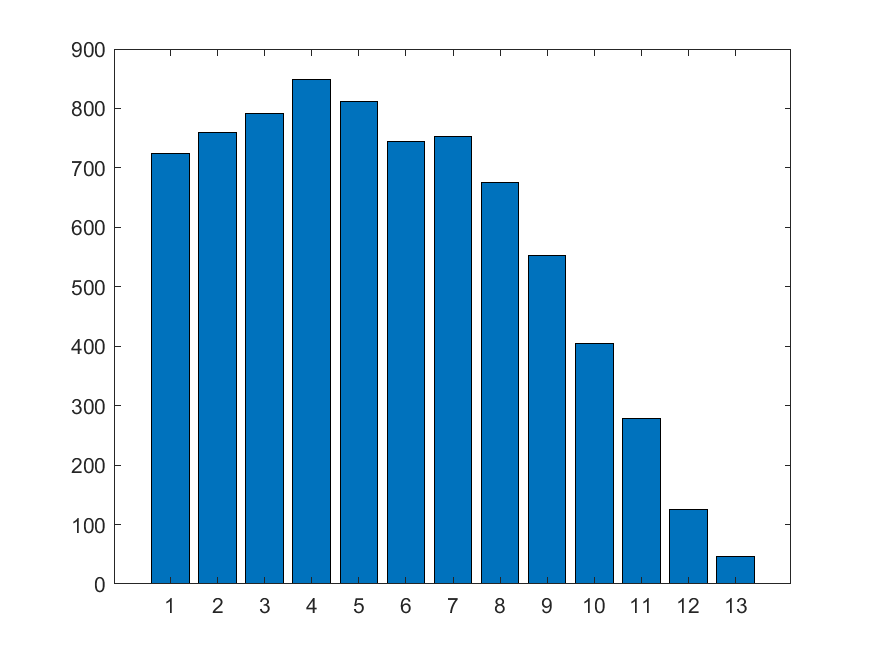
(a) All

(b) Females

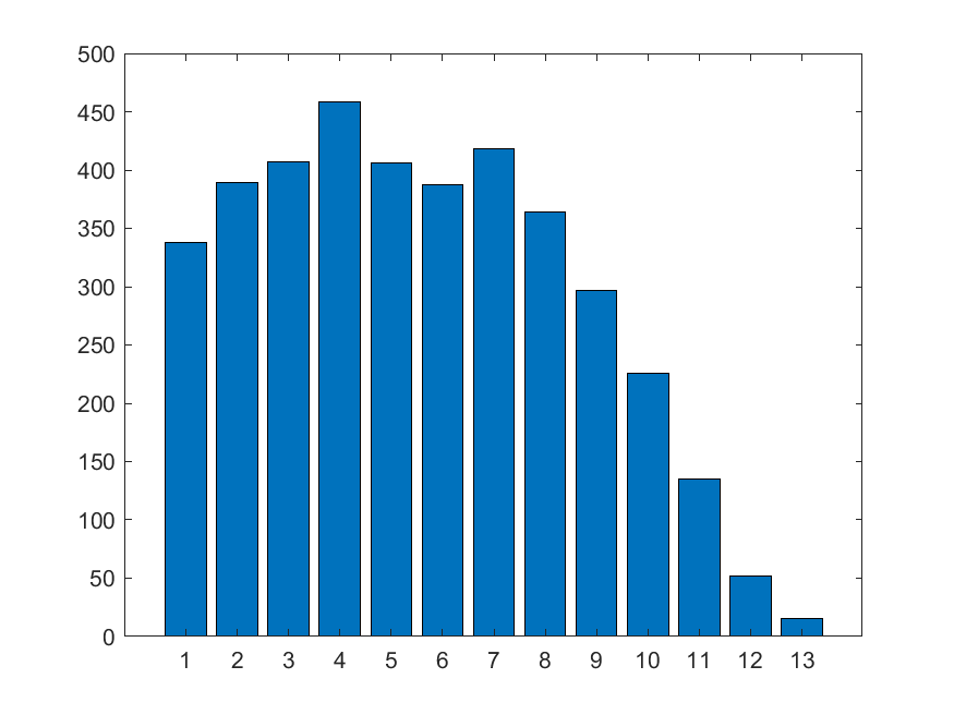
(c) Males

The moment conditions for the fixed effects logit AR(1) in (21) and (44) are all indexed by three time-periods, and they are conditional on the strictly exogenous variables and the initial conditions. One could in principle construct separate conditional moment conditions for each value of $T_{i}$ and each triplet $1\leq t<s<r\leq T_{i}$, and then use them to construct efficient unconditional moment functions. See, for example, the discussion in Newey and McFadden (1994). Unfortunately, the construction of these moment functions depends on the conditional expectation of the derivative of the conditional moment function as well as on the conditional variance of the conditional moment function. We therefore pursue a different approach to obtaining unconditional moment functions. We do not claim that the resulting GMM estimator has any optimality properties, but we have found that it performs well in our Monte Carlo simulations even for relatively small sample sizes, see Appendix B.1 of Honoré and Weidner (2022).

We first normalize all moment functions such that $\sup_{y,x,\beta,\gamma}\allowbreak\left|\widetilde{m}(y,x,\beta,\gamma)\right|<\infty$. For example, the rescaled versions of our $T=3$ moment functions in Section 3.2 are given by

$$\widetilde{m}^{(0)}(y,y_{0},x,\beta,\gamma) = \frac{m^{(0)}(y,y_{0},x,\beta,\gamma)}{1+\exp\left(x_{23}^{\prime}\beta\right)+\exp\left(x_{31}^{\prime}\beta-y_{0}\,\gamma\right)+\exp\left(x_{21}^{\prime}\beta+(1-y_{0})\,\gamma\right)}$$

$$\widetilde{m}^{(1)}(y,y_{0},x,\beta,\gamma) = \frac{m^{(2)}(y,y_{0},x,\beta,\gamma)}{1+\exp\left(x_{12}^{\prime}\beta+y_{0}\,\gamma\right)+\exp\left(x_{13}^{\prime}\beta-(1-y_{0})\,\gamma\right)+\exp\left(x_{32}^{\prime}\beta\right)}$$

Here, each moment function is divided by the sum of the absolute values of all the different positive summands that appear in that moment function. We have found that this rescaling improves the performance of the resulting GMM estimators, particularly for small samples, because it bounds the moment functions and its gradients uniformly over the parameters $\beta$ and $\gamma$. Interestingly, the score functions of the conditional likelihood in Honoré and Kyriazidou (2000) are essentially rescaled in this way.

The rescaled moment functions are valid conditional on any realization of the regressors. We can therefore form unconditional moment functions by multiplying them with arbitrary functions of the regressors and the initial conditions. In our example, we multiply them by 1, the initial condition, and the explanatory variables for the three time periods that index the moment function. For example, for $T=3$, we use

$$M(y,y_{0},x,\beta,\gamma)=\big{(}1,\;y_{0},\;x_{1}^{\prime},\;x_{2}^{\prime},\;x_{3}^{\prime}\big{)}^{\prime}\otimes\left(\begin{array}[]{c}\widetilde{m}^{(1)}(y,y_{0},x,\beta,\gamma)\\ \widetilde{m}^{(0)}(y,y_{0},x,\beta,\gamma)\end{array}\right),$$

where $\otimes$ is the tensor product.

One could in principle construct a moment function for each $\left(t,s,r\right)$ which indexes a moment function. However, this would create a very large number of moment conditions. For a given individual, we therefore add up all the moment functions over all triplets, $t<s<r$. Observations with $T=T_{i}$ time periods will then contribute ${\binom{T_{i}}{3}}$ terms to the sample analog of the moment. This gives very large weight to observations with large $T_{i}$. We therefore weigh the triplets $\left(t,s,r\right)$ for an observation with $T_{i}$ time periods by $\left(T_{i}-1\right)/{\binom{T_{i}}{3}}$. This yields sample moments of the form $\frac{1}{n}\sum_{i=1}^{n}M(Y_{i},Y_{i,0},X_{i},\beta,\gamma)$, and the corresponding GMM estimator is given by

$${\binom{\widehat{\beta}}{\widehat{\gamma}}}=\mathop{\mathrm{a}rgmin}_{\beta\in\mathbb{R}^{K},\,\gamma\in\mathbb{R}}\left(\sum_{i=1}^{n}M(Y_{i},Y_{i,0},X_{i},\beta,\gamma)\right)^{\prime}W\left(\sum_{i=1}^{n}M(Y_{i},Y_{i,0},X_{i},\beta,\gamma)\right),$$

where $W$ is a symmetric positive-definite weight matrix. We use a diagonal weight matrix with the inverse of the moment variances on the diagonal. The motivation stems from Altonji and Segal (1996) who demonstrate that estimating the optimal weighting matrix can result in poor finite sample performance of GMM estimators. They suggest equally weighted moments (i.e., $W=I$) as an alternative. Of course, using equal weights will not be invariant to changes in units, which explains the practice we have adopted.

Under standard regularity conditions we have

$$\sqrt{n}\left[{\binom{\widehat{\beta}}{\widehat{\gamma}}}-{\binom{\beta_{0}}{\gamma_{0}}}\right]\Rightarrow\mathcal{N}\left(0,\,(G^{\prime}WG)^{-1}\,G^{\prime}W\,\Omega\,WG\,(G^{\prime}WG)^{-1}\right),$$

with $\Omega=\mathrm{Var}[m(Y_{i},Y_{i,0},X_{i},\beta_{0},\gamma_{0})]$ and $G=\mathbb{E}\left[\frac{\partial m(Y_{i},Y_{i,0},X_{i},\beta_{0},\gamma_{0})}{\partial\beta^{\prime}},\frac{\partial m(Y_{i},Y_{i,0},X_{i},\beta_{0},\gamma_{0})}{\partial\gamma^{\prime}}\right]$.

Table 1 reports the estimation results. As expected, and consistent with the Monte Carlo results in Appendix B.1 of Honoré and Weidner (2022), the standard logit maximum likelihood estimator of the coefficient on the lagged dependent variable is much larger than the one that estimates a fixed effect for each individual: the estimated fixed effects will be “‘overfitted”, leading to a downward bias in the estimated state dependence. Moreover, the standard logit estimator that ignores fixed effects will capture the presence of persistent heterogeneity by the lagged dependent variable, leading to an upwards bias if such heterogeneity is present in the data. The GMM estimator gives a much smaller coefficient than the standard logit maximum likelihood estimator, suggesting that heterogeneity plays a big role in this application.

Table 1: Empirical Results (AR(1)).

	Females				Males				All
	Logit	Logit w FE	GMM		Logit	Logit w FE	GMM		Logit	Logit w FE	GMM
Lagged $y$	$2.585$	$0.780$	$1.512$		$2.947$	$0.709$	$1.454$		$2.797$	$0.768$	$1.417$
	$(0.038\hbox to0.0pt{)\hss}$	$(0.050\hbox to0.0pt{)\hss}$	$(0.076\hbox to0.0pt{)\hss}$		$(0.040\hbox to0.0pt{)\hss}$	$(0.063\hbox to0.0pt{)\hss}$	$(0.088\hbox to0.0pt{)\hss}$		$(0.027\hbox to0.0pt{)\hss}$	$(0.039\hbox to0.0pt{)\hss}$	$(0.060\hbox to0.0pt{)\hss}$
Children	$-0.335$	$-0.444$	$-0.244$		$-0.153$	$0.018$	$-0.275$		$-0.278$	$-0.252$	$-0.214$
	$(0.016\hbox to0.0pt{)\hss}$	$(0.052\hbox to0.0pt{)\hss}$	$(0.196\hbox to0.0pt{)\hss}$		$(0.021\hbox to0.0pt{)\hss}$	$(0.067\hbox to0.0pt{)\hss}$	$(0.133\hbox to0.0pt{)\hss}$		$(0.012\hbox to0.0pt{)\hss}$	$(0.043\hbox to0.0pt{)\hss}$	$(0.102\hbox to0.0pt{)\hss}$
Married	$0.082$	$-0.044$	$0.637$		$0.335$	$0.332$	$0.038$		$0.349$	$0.173$	$0.707$
	$(0.084\hbox to0.0pt{)\hss}$	$(0.159\hbox to0.0pt{)\hss}$	$(0.890\hbox to0.0pt{)\hss}$		$(0.071\hbox to0.0pt{)\hss}$	$(0.171\hbox to0.0pt{)\hss}$	$(0.295\hbox to0.0pt{)\hss}$		$(0.053\hbox to0.0pt{)\hss}$	$(0.111\hbox to0.0pt{)\hss}$	$(0.397\hbox to0.0pt{)\hss}$
SP.Inc.	$-0.010$	$-0.050$	$-0.104$		$0.033$	$0.003$	$0.019$		$-0.017$	$-0.044$	$-0.089$
	$(0.006\hbox to0.0pt{)\hss}$	$(0.011\hbox to0.0pt{)\hss}$	$(0.068\hbox to0.0pt{)\hss}$		$(0.007\hbox to0.0pt{)\hss}$	$(0.016\hbox to0.0pt{)\hss}$	$(0.026\hbox to0.0pt{)\hss}$		$(0.004\hbox to0.0pt{)\hss}$	$(0.009\hbox to0.0pt{)\hss}$	$(0.033\hbox to0.0pt{)\hss}$

• The estimation also includes 12 time dummies. Standard error for the GMM and Logit Fixed Effects Estimators are calculated as the interquartile range of 1,000 bootstrap replications divided by 1.35.

Table 2: Empirical Results (AR(2)).

	Females				Males				All
	Logit	Logit w FE	GMM		Logit	Logit w FE	GMM		Logit	Logit w FE	GMM
$y_{t-1}$	$2.259$	$0.742$	$1.356$		$2.422$	$0.514$	$1.116$		$2.361$	$0.665$	$1.297$
	$(0.047\hbox to0.0pt{)\hss}$	$(0.069\hbox to0.0pt{)\hss}$	$(0.162\hbox to0.0pt{)\hss}$		$(0.052\hbox to0.0pt{)\hss}$	$(0.083\hbox to0.0pt{)\hss}$	$(0.131\hbox to0.0pt{)\hss}$		$(0.035\hbox to0.0pt{)\hss}$	$(0.053\hbox to0.0pt{)\hss}$	$(0.092\hbox to0.0pt{)\hss}$
$y_{t-2}$	$0.917$	$-0.379$	$0.678$		$1.332$	$-0.286$	$0.558$		$1.137$	$-0.319$	$0.648$
	$(0.048\hbox to0.0pt{)\hss}$	$(0.072\hbox to0.0pt{)\hss}$	$(0.081\hbox to0.0pt{)\hss}$		$(0.053\hbox to0.0pt{)\hss}$	$(0.080\hbox to0.0pt{)\hss}$	$(0.066\hbox to0.0pt{)\hss}$		$(0.036\hbox to0.0pt{)\hss}$	$(0.054\hbox to0.0pt{)\hss}$	$(0.046\hbox to0.0pt{)\hss}$
Children	$-0.260$	$-0.410$	$-1.926$		$-0.143$	$0.112$	$-0.188$		$-0.223$	$-0.192$	$-1.209$
	$(0.018\hbox to0.0pt{)\hss}$	$(0.069\hbox to0.0pt{)\hss}$	$(0.282\hbox to0.0pt{)\hss}$		$(0.024\hbox to0.0pt{)\hss}$	$(0.100\hbox to0.0pt{)\hss}$	$(0.251\hbox to0.0pt{)\hss}$		$(0.014\hbox to0.0pt{)\hss}$	$(0.051\hbox to0.0pt{)\hss}$	$(0.219\hbox to0.0pt{)\hss}$
Married	$0.136$	$0.022$	$-0.193$		$0.411$	$0.534$	$-0.019$		$0.393$	$0.269$	$-0.121$
	$(0.095\hbox to0.0pt{)\hss}$	$(0.184\hbox to0.0pt{)\hss}$	$(0.028\hbox to0.0pt{)\hss}$		$(0.083\hbox to0.0pt{)\hss}$	$(0.203\hbox to0.0pt{)\hss}$	$(0.025\hbox to0.0pt{)\hss}$		$(0.061\hbox to0.0pt{)\hss}$	$(0.145\hbox to0.0pt{)\hss}$	$(0.022\hbox to0.0pt{)\hss}$
Sp.Inc	$-0.015$	$-0.050$	$0.255$		$0.023$	$-0.008$	$0.179$		$-0.022$	$-0.046$	$0.093$
	$(0.007\hbox to0.0pt{)\hss}$	$(0.014\hbox to0.0pt{)\hss}$	$(0.210\hbox to0.0pt{)\hss}$		$(0.008\hbox to0.0pt{)\hss}$	$(0.019\hbox to0.0pt{)\hss}$	$(0.316\hbox to0.0pt{)\hss}$		$(0.005\hbox to0.0pt{)\hss}$	$(0.011\hbox to0.0pt{)\hss}$	$(0.183\hbox to0.0pt{)\hss}$

• The estimation also includes 11 time dummies. Standard error for the GMM and Logit Fixed Effects Estimators are calculated as the interquartile range of 1,000 bootstrap replications divided by 1.35.

To estimate the AR(2) version of the model, we apply the moment conditions provided in Appendix A.3.1 to all consecutive sequences of six outcomes (treating the first two as initial conditions). The moment functions are scaled as described in the Monte Carlo simulations in Appendix B.1 of Honoré and Weidner (2022). The results are presented in Table 2. The most interesting finding is that for all three samples, the GMM estimator of $\left(\gamma_{1},\gamma_{2}\right)$ is between the maximum likelihood estimator that ignores the fixed effects, and the one that estimates a fixed effect for each individual. This suggests that unobserved individual-specific heterogeneity is important in this example. Economically, it is also interesting that for each estimation method, the estimates of $\left(\gamma_{1},\gamma_{2}\right)$ are quite similar across the three samples.

8 Conclusion

Bonhomme (2012) proposed a general approach for constructing moment restrictions in nonlinear panel data models that do not depend on individual-specific effects. In this paper, we have operationalized this in models with discrete outcomes by first presenting a blueprint for deciding whether such moment conditions exist, and then an approach for actually finding analytic expressions for the moment conditions.

We have used our approach to derive all the moment conditions for the panel logit AR(1) model that are free of the fixed effects, and we have employed those moment conditions to show identification of the common model parameters and to obtain a GMM estimator that is useful and performs well in practice. The immediate practical relevance of this paper is therefore for the dynamic panel logit model (both AR(1) and AR(2) models are estimated in an empirical application).

While part of this paper emphasises binary logit models, the methods explained in Section 2 and 3 for exploring and deriving moment conditions are applicable for more general panel models, as illustrated by the examples provided in Section 4. Exploring such moment conditions in other interesting models is a research agenda that has only started (e.g. Honoré, Muris, and Weidner 2021, Davezies, D’Haultfoeuille, and Mugnier 2022), and a lot more future work should be done to provide useful new estimation methods in various discrete choice panel models.

Appendix A Online Appendix (not for publication)

A.1 Proofs of main text results

Lemma 1 is a special case of Theorem 2, which is proven below. Alternatively, Lemma 1 can be proved more directly by “brute-force calculations”, see Appendix B.2.1 if Honoré and Weidner (2022) of the supplementary appendix.

Proof of Lemma 2. The lemma holds trivially for $K=0$ when $s=\emptyset$ and $g_{\emptyset}:\mathbb{R}\rightarrow\mathbb{R}$ is a single increasing function, implying that $g_{\emptyset}(\gamma)=0$ can at most have one solution. Consider $K\geq 1$ in the following. We follow a proof by contradiction. Assume that $(\beta_{1},\gamma_{1})\in\mathbb{R}^{K}\times\mathbb{R}$ and $(\beta_{2},\gamma_{2})\in\mathbb{R}^{K}\times\mathbb{R}$ both solve $g_{s}(\beta_{1},\gamma_{1})=0$ and $g_{s}(\beta_{2},\gamma_{2})=0$, for all $s\in\{-,+\}^{K}$, with $(\beta_{1},\gamma_{1})\neq(\beta_{2},\gamma_{2})$. Our goal is to derive a contradiction between this and the assumptions of the lemma. Without loss of generality, we assume that $\gamma_{1}\leq\gamma_{2}$. Define $s^{\ast}\in\{-,+\}^{K}$ by

$$s_{k}^{\ast}=\left\{\begin{array}[]{ll}+&\text{if}\;\beta_{1,k}\leq\beta_{2,k},\\ -&\text{otherwise,}\end{array}\right.$$

for all $k\in\{1,\ldots,K\}$. By the monotonicity assumptions on $g_{s}(\beta,\gamma)$ in the lemma, we have that $g_{s^{\ast}}(\beta,\gamma)$ is strictly increasing in $\gamma$ and we have $\gamma_{1}\leq\gamma_{2}$; if $s_{k}^{\ast}=+$, then $g_{s^{\ast}}(\beta,\gamma)$ is strictly increasing in $\beta_{k}$ and we have $\beta_{1,k}\leq\beta_{2,k}$; and if $s_{k}^{\ast}=-$, then $g_{s^{\ast}}(\beta,\gamma)$ is strictly decreasing in $\beta_{k}$ and we have $\beta_{1,k}>\beta_{2,k}$. Furthermore, one of these inequalities on the parameters must be strict, because we have $(\beta_{1},\gamma_{1})\neq(\beta_{2},\gamma_{2})$. We therefore conclude that

$$g_{s^{\ast}}(\beta_{1},\gamma_{1})<g_{s^{\ast}}(\beta_{2},\gamma_{2}).$$

This violates the assumption that $g_{s}(\beta_{1},\gamma_{1})=0$ and $g_{s}(\beta_{2},\gamma_{2})=0$. Thus, under the assumptions of the lemma there cannot be two solutions of the system (26).    

Proof of Theorem 1. Consider $y_{0}=0$ and $q=0$. Using the definition of the moment function $m^{(0)}(y,y_{0},x,\beta,\gamma)$ in Section 3.2 and the distribution of $Y|X,A$ implied by model (2) we find

$$\frac{\partial\,\overline{m}_{0,s}^{(0)}(\beta,\gamma)}{\partial\gamma} =\mathbb{E}\left[\left.\frac{\partial\,m^{(0)}(Y,0,X,\beta,\gamma)}{\partial\gamma}\,\right|\,Y_{0}=0,\;X\in\mathcal{X}_{s}\right]$$

$$=\mathbb{E}\left[\left.\frac{\partial\,\exp\left(\gamma+X_{21}^{\prime}\beta\right)}{\partial\gamma}\,{\mathrm{P}r}\left[Y=(1,0,1)\,\big{|}\,Y_{0}=0,X,A\right]\,\right|\,Y_{0}=0,\;X\in\mathcal{X}_{s}\right]$$

$$=\mathbb{E}\left[\left.\exp\left(\gamma+X_{21}^{\prime}\beta\right)\,p((1,0,1),0,X,\beta_{0},\gamma_{0},A)\,\right|\,Y_{0}=0,\;X\in\mathcal{X}_{s}\right]>0,$$

where in the last step (to conclude that the expression is positive) we used that $\,p((1,0,1),0,x,\beta_{0},\gamma_{0},\alpha)>0$ for all $x\in\mathbb{R}^{K\times 3}$ and $\alpha\in\mathbb{R}$. We have thus shown that $\overline{m}_{0,s}^{(0)}(\beta,\gamma)$ is strictly increasing in $\gamma$. Analogously, one can show that $\overline{m}_{0,s}^{(0)}(\beta,\gamma)$ is strictly increasing in $\beta_{k}$ if $s_{k}=+$, and strictly decreasing in $\beta_{k}$ if $s_{k}=-$, for all $k\in\{1,\ldots,K\}$, because of the result in (27) above.

We can therefore apply Lemma 2 with $g_{s}(\beta,\gamma)$ equal to $\overline{m}_{0,s}^{(0)}(\beta,\gamma)$ to find that the system of equations in (28) has at most one solution. Using Lemma 1 we find that such a solution exists and is given by $(\beta_{0},\gamma_{0})$.

For the other values of $q,y_{0}\in\{0,1\}$ we can analogously apply Lemma 2 with $g_{s}(\beta,\gamma)$ equal to $\overline{m}^{(0)}_{1,s}(\beta,-\gamma)$, $\overline{m}^{(1)}_{0,s}(-\beta,-\gamma)$, $\overline{m}^{(1)}_{1,s}(-\beta,\gamma)$, respectively.    

Key intermediate result for the proof of Lemma 3 and Theorem 2

Lemma 4 below is a slight reformulation and generalization of Lemma 3 in the main text. Once we have established Lemma 4, then the proofs of both Lemma 3 and Theorem 2 are straightforward. To present Lemma 4, it is useful to first introduce some additional notation:

Let $\widetilde{Y}_{1},\widetilde{Y}_{2},\widetilde{Y}_{3}\in\{0,1\}$, $W_{2}\in{\cal W}_{2}$, and $W_{3}\in{\cal W}_{3}$ be random variables. Let $\widetilde{Y}=(\widetilde{Y}_{1},\widetilde{Y}_{2},\widetilde{Y}_{3})$, and let $p(\widetilde{y},w_{2},w_{3})\in[0,\infty)$ describe the joint distribution of $(\widetilde{Y},W_{2},W_{3})$, that is, for all measurable subsets ${\cal Y}_{*}\subset\{0,1\}^{3}$, ${\cal W}^{*}_{2}\subset{\cal W}_{2}$ and ${\cal W}^{*}_{3}\subset{\cal W}_{3}$ we have

$${\mathrm{P}r}\left(\widetilde{Y}\in{\cal Y}_{*}\;\;\&\;\;W_{2}\in{\cal W}^{*}_{2}\;\;\&\;\;W_{3}\in{\cal W}^{*}_{3}\right) =\sum_{\widetilde{y}\in{\cal Y}_{*}}\int_{w_{2}\in{\cal W}^{*}_{2}}\int_{w_{3}\in{\cal W}^{*}_{3}}\,p(\widetilde{y},w_{2},w_{3})\,\mu(dw_{2})\,\nu(dw_{3}),$$

for appropriate probability measures $\mu$ and $\nu$ on ${\cal W}_{2}$ and ${\cal W}_{3}$. We assume that we can decompose the joint distribution of $\widetilde{Y}$, $W_{2}$, $W_{3}$ as follows,

$$p(\widetilde{y},w_{2},w_{3}) =p_{3}(\widetilde{y}_{3}\,|\,w_{3})\;\,g(w_{3}\,|\,\widetilde{y}_{2},w_{2})\;\,p_{2}(\widetilde{y}_{2}\,|\,w_{2})\;\,f(w_{2}\,|\,\widetilde{y}_{1})\;\,p_{1}(\widetilde{y}_{1}),$$ (61)

where $\widetilde{y}=(\widetilde{y}_{1},\widetilde{y}_{2},\widetilde{y}_{3})$, the functions $p_{3}$, $g$, $p_{2}$, $f$ are appropriate transition probabilities/densities, and $p_{1}(\widetilde{y}_{1})={\mathrm{P}r}\left(\widetilde{Y}_{1}=\widetilde{y}_{1}\right)$ is the marginal distribution of $\widetilde{Y}_{1}$. For $p_{1}(\widetilde{y}_{1})$, $p_{2}(\widetilde{y}_{2}\,|\,w_{2})$, $p_{3}(\widetilde{y}_{3}\,|\,w_{3})$ we impose:

$$p_{1}(\widetilde{y}_{1}) =\Lambda\left[(2\,\widetilde{y}_{1}-1)\,\pi_{1}\right],$$

$$p_{2}(\widetilde{y}_{2}\,|\,w_{2}) =\Lambda\left[(2\,\widetilde{y}_{2}-1)\,\pi_{2}(w_{2})\right],$$

$$p_{3}(\widetilde{y}_{3}\,|\,w_{3}) =\Lambda\left[(2\,\widetilde{y}_{3}-1)\,\pi_{3}(w_{3})\right],$$ (62)

where $\Lambda(\xi):=[1+\exp(-\xi)]^{-1}$ is the cumulative distribution function of the logistic distribution, $\pi_{1}\in\mathbb{R}$ is a constant, and $\pi_{2}:\,{\cal W}_{2}\rightarrow\mathbb{R}$ and $\pi_{3}:\,{\cal W}_{3}\rightarrow\mathbb{R}$ are functions. The only assumption that we impose on $f(w_{2}\,|\,\widetilde{y}_{1})$ and $g(w_{3}\,|\,\widetilde{y}_{2},w_{2})$ is that

$$g(w_{3}\,|\,1,w_{2})=g(w_{3}\,|\,1),$$ (63)

that is, conditional on $\widetilde{Y}_{2}=1$, the distribution of $W_{3}$ is independent of $W_{2}$. Apart from that, we only require that $f(w_{2}\,|\,\widetilde{y}_{1})$ and $g(w_{3}\,|\,\widetilde{y}_{2},w_{2})$ are conditional probability distributions, which sum to one:

$$\int_{w_{2}\in{\cal W}_{2}}\,f(w_{2}\,|\,\widetilde{y}_{1})\,\mu(dw_{2}) =1, \int_{w_{3}\in{\cal W}_{3}}\,g(w_{3}\,|\,\widetilde{y}_{2},w_{2})\,\nu(dw_{3}) =1.$$ (64)

Note that if we would strengthen (63) to $g(w_{3}\,|\,\widetilde{y}_{2},w_{2})=g(w_{3}\,|\,\widetilde{y}_{2})$, for $\widetilde{y}_{2}\in\{0,1\}$, then (61) would be equivalent to the Markov chain condition imposed in Lemma 3 ($\widetilde{Y}_{1}\overset{f}{\longrightarrow}W_{2}\overset{p_{2}}{\longrightarrow}\widetilde{Y}_{2}\overset{g}{\longrightarrow}W_{3}\overset{p_{3}}{\longrightarrow}\widetilde{Y}_{3}$). However, since here we only impose (63), we also allow for dependence of $W_{2}$ and $W_{3}$, conditional on $\widetilde{Y}_{2}=0$. This generalization to a non-Markovian structure is crucial for the ordered logit model in Honoré, Muris, and Weidner (2021), but is less important for the binary logit model discussed in this paper (See Appendix A.2 below for further discussion). Finally, we define $m:\{0,1\}^{3}\times{\cal W}_{2}\times{\cal W}_{3}\rightarrow\mathbb{R}$ by

$$m(\widetilde{y},w_{2},w_{3}) :=\left\{\begin{array}[]{ll}\exp\left[\pi_{1}-\pi_{2}(w_{2})\right]&\text{if }\widetilde{y}=(0,1,0),\\ \exp\left[\pi_{1}-\pi_{3}(w_{3})\right]&\text{if }\widetilde{y}=(0,1,1),\\ -1&\text{if }(\widetilde{y}_{1},\widetilde{y}_{2})=(1,0),\\ \exp\left[\pi_{3}(w_{3})-\pi_{2}(w_{2})\right]-1&\text{if }\widetilde{y}=(1,1,0),\\ 0&\text{otherwise}.\end{array}\right.$$ (70)

Lemma 4

Let $\pi_{1}\in\mathbb{R}$, $\pi_{2}:\,{\cal W}_{2}\rightarrow\mathbb{R}$ and $\pi_{3}:\,{\cal W}_{3}\rightarrow\mathbb{R}$. Let the random variables $\widetilde{Y}\in\{0,1\}^{3}$, $W_{2}\in{\cal W}_{2}$, $W_{3}\in{\cal W}_{3}$ be such that their distributions satisfy (61), (62), (63), (64), and let $m:\{0,1\}^{3}\times{\cal W}_{2}\times{\cal W}_{3}\rightarrow\mathbb{R}$ be defined by (70). Then we have

$$\mathbb{E}\left[m(\widetilde{Y},W_{2},W_{3})\right]=0.$$

Proof. Define

$$h(\widetilde{y}_{1},\widetilde{y}_{2},w_{2},w_{3}) :=\,\sum_{\widetilde{y}_{3}\in\{0,1\}}\,m(\widetilde{y},w_{2},w_{3})\;\,p_{3}(\widetilde{y}_{3}\,|\,w_{3})\;\,p_{2}(\widetilde{y}_{2}\,|\,w_{2})\;\,p_{1}(\widetilde{y}_{1}),$$

where $\widetilde{y}=(\widetilde{y}_{1},\widetilde{y}_{2},\widetilde{y}_{3})$. By using the expressions for the functions $p_{1}$, $p_{2}$, $p_{3}$, and $m$ in (62) and (70) we find that

$$h(\widetilde{y}_{1},\widetilde{y}_{2},w_{2},w_{3}) =\left\{\begin{array}[]{ll}\Lambda(\pi_{1})\,\Lambda[-\pi_{3}(w_{3})]&\text{if }(\widetilde{y}_{1},\widetilde{y}_{2})=(0,1),\\ -p_{2}(\widetilde{y}_{2}\,|\,w_{2})\,p_{1}(\widetilde{y}_{1})&\text{if }(\widetilde{y}_{1},\widetilde{y}_{2})=(1,0),\\ \Lambda(\pi_{1})\,\Lambda[\pi_{3}(w_{3})]\,-p_{2}(\widetilde{y}_{2}\,|\,w_{2})\,p_{1}(\widetilde{y}_{1})&\text{if }(\widetilde{y}_{1},\widetilde{y}_{2})=(1,1),\\ 0&\text{otherwise},\end{array}\right.$$

$$=\underbrace{\mathbbm{1}\left\{\widetilde{y}_{2}=1\right\}\,\Lambda(\pi_{1})\,\Lambda[(2\widetilde{y}_{1}-1)\pi_{3}(w_{3})]}_{\displaystyle=:h_{1}(\widetilde{y}_{1},\widetilde{y}_{2},w_{3})}\,\underbrace{-\,\mathbbm{1}\left\{\widetilde{y}_{1}=1\right\}\,p_{2}(\widetilde{y}_{2}\,|\,w_{2})\,p_{1}(\widetilde{y}_{1})}_{\displaystyle=:h_{2}(\widetilde{y}_{1},\widetilde{y}_{2},w_{2})},$$

where we have decomposed $h(\widetilde{y}_{1},\widetilde{y}_{2},w_{2},w_{3})$ into the sum of $h_{1}(\widetilde{y}_{1},\widetilde{y}_{2},w_{3})$, which does not depend on $w_{2}$, and of $h_{2}(\widetilde{y}_{1},\widetilde{y}_{2},w_{2})$, which does not depend on $w_{3}$. Note that the term $\Lambda[(2\widetilde{y}_{1}-1)\pi_{3}(w_{3})]$ in $h_{1}(\widetilde{y}_{1},\widetilde{y}_{2},w_{3})$ is identical to $p_{3}(\widetilde{y}_{3}\,|\,w_{3})$, but with $\widetilde{y}_{3}$ replaced by $\widetilde{y}_{1}$. Also using (63) and (64) we find

$$\sum_{\widetilde{y}_{1}\in\{0,1\}}\sum_{\widetilde{y}_{2}\in\{0,1\}}\int_{w_{2}\in{\cal W}_{2}}\,\int_{w_{3}\in{\cal W}_{3}}\,h_{1}(\widetilde{y}_{1},\widetilde{y}_{2},w_{3})\;\,g(w_{3}\,|\,\widetilde{y}_{2},w_{2})\;\,f(w_{2}\,|\,\widetilde{y}_{1})\,\mu(dw_{2})\,\nu(dw_{3})$$

$$=\Lambda(\pi_{1})\sum_{\widetilde{y}_{1}\in\{0,1\}}\int_{w_{2}\in{\cal W}_{2}}\,\int_{w_{3}\in{\cal W}_{3}}\,\,\Lambda[(2\widetilde{y}_{1}-1)\pi_{3}(w_{3})]\;\,g(w_{3}\,|\,1)\;\,f(w_{2}\,|\,\widetilde{y}_{1})\;\,\,\mu(dw_{2})\,\nu(dw_{3})$$

$$=\Lambda(\pi_{1})\sum_{\widetilde{y}_{1}\in\{0,1\}}\int_{w_{3}\in{\cal W}_{3}}\,\Lambda[(2\widetilde{y}_{1}-1)\pi_{3}(w_{3})]\;\,g(w_{3}\,|\,1)\,\underbrace{\int_{w_{2}\in{\cal W}_{2}}\,f(w_{2}\,|\,\widetilde{y}_{1})\,\mu(dw_{2})}_{=1}\,\nu(dw_{3})$$

$$=\Lambda(\pi_{1})\int_{w_{3}\in{\cal W}_{3}}\underbrace{\sum_{\widetilde{y}_{1}\in\{0,1\}}\,\Lambda[(2\widetilde{y}_{1}-1)\pi_{3}(w_{3})]}_{=1}\;\,g(w_{3}\,|\,1)\,\nu(dw_{3})$$

$$=\Lambda(\pi_{1})\underbrace{\int_{w_{3}\in{\cal W}_{3}}\,g(w_{3}\,|\,1)\,\nu(dw_{3})}_{=1}$$

$$=\Lambda(\pi_{1}).$$

Similarly, we calculate

$$\sum_{\widetilde{y}_{1}\in\{0,1\}}\sum_{\widetilde{y}_{2}\in\{0,1\}}\int_{w_{2}\in{\cal W}_{2}}\,\int_{w_{3}\in{\cal W}_{3}}\,h_{2}(\widetilde{y}_{1},\widetilde{y}_{2},w_{2})\;\,g(w_{3}\,|\,\widetilde{y}_{2},w_{2})\;\,f(w_{2}\,|\,\widetilde{y}_{1})\,\mu(dw_{2})\,\nu(dw_{3})$$

$$=\sum_{\widetilde{y}_{1}\in\{0,1\}}\sum_{\widetilde{y}_{2}\in\{0,1\}}\int_{w_{2}\in{\cal W}_{2}}\,h_{2}(\widetilde{y}_{1},\widetilde{y}_{2},w_{2})\underbrace{\int_{w_{3}\in{\cal W}_{3}}\,g(w_{3}\,|\,\widetilde{y}_{2},w_{2})\,\nu(dw_{3})}_{=1}f(w_{2}\,|\,\widetilde{y}_{1})\,\mu(dw_{2})$$

$$=-\,p_{1}(1)\int_{w_{2}\in{\cal W}_{2}}\,\underbrace{\sum_{\widetilde{y}_{2}\in\{0,1\}}p_{2}(\widetilde{y}_{2}\,|\,w_{2})}_{=1}\;\,f(w_{2}\,|\,1)\,\mu(dw_{2})$$

$$=-\,p_{1}(1)\underbrace{\int_{w_{2}\in{\cal W}_{2}}\,f(w_{2}\,|\,1)\,\mu(dw_{2})}_{=1}$$

$$=-\,\Lambda(\pi_{1}).$$

Combining the results in the last two displays gives

$$\sum_{\widetilde{y}_{1}\in\{0,1\}}\sum_{\widetilde{y}_{2}\in\{0,1\}}\int_{w_{2}\in{\cal W}_{2}}\,\int_{w_{3}\in{\cal W}_{3}}\,h(\widetilde{y}_{1},\widetilde{y}_{2},w_{2},w_{3})\;\,g(w_{3}\,|\,\widetilde{y}_{2},w_{2})\;\,f(w_{2}\,|\,\widetilde{y}_{1})\,\mu(dw_{2})\,\nu(dw_{3})=0,$$

and by the definition of $h(\widetilde{y}_{1},\widetilde{y}_{2},w_{2},w_{3})$ this is equivalent to $\mathbb{E}\left[m(\widetilde{Y},W_{2},W_{3})\right]=0$, which is what we wanted to show.    

We are now ready to prove the remaining main text results.

Proof of Lemma 3. Let the assumptions of Lemma 3 hold. We are going to verify that this implies that all the assumptions of Lemma 4 hold, conditional on $(W_{1},X,A)$. We condition on $(W_{1},X,A)=(w_{1},x,a)$ in all the following stochastic statements, and when verifying the assumptions of Lemma 4, we write $p_{t}(\widetilde{y}_{t}\,|\,w_{t},x,\alpha)$, $t\in\{1,2,3\}$, instead of $p_{1}(\widetilde{y}_{1})$, $p_{2}(\widetilde{y}_{2}\,|\,w_{2})$, $p_{3}(\widetilde{y}_{3}\,|\,w_{3})$. The additional arguments $w_{1}$, $x$, $a$ do not matter here, since they are held constant (i.e. conditioned on). By the same argument, we write $\pi_{t}(w_{t},x,\alpha)$, $t\in\{1,2,3\}$, here instead of $\pi_{1}$, $\pi_{2}(w_{2})$, $\pi_{3}(w_{3})$. The Markov chain assumption in Lemma 3 implies that conditions (61) and (63) hold. For $t\in\{1,2,3\}$ we define

$$\pi_{t}(w_{t},x,\alpha):=\Lambda^{-1}\Big{[}p_{t}\left(1\,\big{|}\,w_{t},x,\alpha\right)\Big{]},$$ (71)

which guarantees that (62) holds. Finally, (64) is satisfied for any conditional probability. We can thus apply Lemma 4 to find that

$$\mathbb{E}\left[m^{(1)}(w_{1},\widetilde{Y}_{1},W_{2},\widetilde{Y}_{2},W_{3},\widetilde{Y}_{3},x,a)\,\Big{|}\,W_{1}=w_{1},\,X=x,\,A=a\right]=0,$$

where $m^{(1)}(w_{1},\widetilde{y}_{1},w_{2},\widetilde{y}_{2},w_{3},\widetilde{Y}_{3},x,a)$ is equal to $m(\widetilde{y},w_{2},w_{3})$ defined in (70), with $\widetilde{y}=(\widetilde{y}_{1},\widetilde{y}_{2},\widetilde{y}_{3})$, and with the additional arguments $w_{1}$, $x$, $a$ added through $\pi_{t}(w_{t},x,\alpha)$, as explained above, that is,

$$m^{(1)}(w_{1},\widetilde{y}_{1},w_{2},\widetilde{y}_{2},w_{3},\widetilde{y}_{3},x,\alpha)$$

$$\quad=\left\{\begin{array}[]{ll}\exp\left[\pi_{1}(w_{1},x,\alpha)-\pi_{2}(w_{2},x,\alpha)\right]&\text{if }\widetilde{y}=(0,1,0),\\ \exp\left[\pi_{1}(w_{1},x,\alpha)-\pi_{3}(w_{3},x,\alpha)\right]&\text{if }\widetilde{y}=(0,1,1),\\ -1&\text{if }(\widetilde{y}_{1},\widetilde{y}_{2})=(1,0),\\ \exp\left[\pi_{3}(w_{3},x,\alpha)-\pi_{2}(w_{2},x,\alpha)\right]-1&\text{if }\widetilde{y}=(1,1,0),\\ 0&\text{otherwise},\end{array}\right.$$

$$\quad=-\mathbbm{1}\left\{\widetilde{y}_{1}=1\right\}+\left\{\begin{array}[]{ll}\exp\left[\pi_{1}(w_{1},x,\alpha)-\pi_{2}(w_{2},x,\alpha)\right]&\text{if }\widetilde{y}=(0,1,0),\\ \exp\left[\pi_{1}(w_{1},x,\alpha)-\pi_{3}(w_{3},x,\alpha)\right]&\text{if }\widetilde{y}=(0,1,1),\\ \exp\left[\pi_{3}(w_{3},x,\alpha)-\pi_{2}(w_{2},x,\alpha)\right]&\text{if }\widetilde{y}=(1,1,0),\\ 1&\text{if }\widetilde{y}=(1,1,1),\\ 0&\text{otherwise},\end{array}\right.$$

$$\quad=-\mathbbm{1}\left\{\widetilde{y}_{1}=1\right\}$$

$$\qquad+\mathbbm{1}\left\{\widetilde{y}_{2}=1\right\}\,\exp\left\{\sum_{t=1}^{3}\widetilde{y}_{t}\bigg{[}\pi_{\delta(t)}\left(w_{\delta(t)},x,\alpha\right)-\pi_{t}(w_{t},x,\alpha)\bigg{]}\right\}$$

$$\quad=-\mathbbm{1}\left\{\widetilde{y}_{1}=1\right\}$$

$$\qquad+\mathbbm{1}\left\{\widetilde{y}_{2}=1\right\}\,\exp\left\{\frac{1}{2}\sum_{t=1}^{3}(2\widetilde{y}_{t}-1)\bigg{[}\pi_{\delta(t)}\left(w_{\delta(t)},x,\alpha\right)-\pi_{t}(w_{t},x,\alpha)\bigg{]}\right\}$$

$$\quad=-\mathbbm{1}\left\{\widetilde{y}_{1}=1\right\}$$

$$\qquad+\mathbbm{1}\left\{\widetilde{y}_{2}=1\right\}\,\exp\left(\frac{1}{2}\sum_{t=1}^{3}\bigg{\{}\Lambda^{-1}\Big{[}p_{\delta(t)}\left(\widetilde{y}_{t}\,\big{|}\,w_{\delta(t)},x,\alpha\right)\Big{]}-\Lambda^{-1}\Big{[}p_{t}\left(\widetilde{y}_{t}\,\big{|}\,w_{t},x,\alpha\right)\Big{]}\bigg{\}}\right),$$

where in the last step we used that (71) together with $\sum_{y\in\{0,1\}}p_{t}\left(y\big{|}w_{t},x,\alpha\right)=1$ implies that $p_{t}\left(y\big{|}w_{t},x,\alpha\right)=\Lambda[(2y-1)\,\pi\left(w_{t},x,\alpha\right)]$, for all $y\in\{0,1\}$ and $t\in\{1,2,3\}$. We have therefore shown the result of Lemma 3 for $q=1$. The result for $q=0$ directly follows from this by applying the symmetry transformation $\widetilde{y}_{t}\,\leftrightarrow\,1-\widetilde{y}_{t}$, and $\pi_{t}(w_{t},x,\alpha)\,\leftrightarrow\,-\pi_{t}(w_{t},x,\alpha)$.    

Proof of Theorem 2. Let the assumptions of Theorem 2 be satisfied. By choosing $(\widetilde{Y}_{1},\widetilde{Y}_{2},\widetilde{Y}_{3})=(Y_{t},Y_{s},Y_{r})$ and $(W_{1},W_{2},W_{3})=(Y_{t-1},Y_{s-1},Y_{r-1})$, it is then easy to verify that the conditions of Lemma 3 are satisfied, when conditioning on $(X,A,Y_{0},\,Y_{1},\ldots\allowbreak,\allowbreak Y_{t-1})$. The only substantial assumption to verify here is the Markov chain condition, which immediately follows from the AR(1) structure of $Y_{t}$. The panel AR(1) model restriction in (2) (after dropping the index $i$) then implies that the moment function $m^{(q)}(w_{1},\widetilde{y}_{1},w_{2},\widetilde{y}_{2},w_{3},\widetilde{y}_{3},x,\alpha)$ in the lemma now reads

$$m^{(q)(t,s,r)}(y,y_{0},x,\beta_{0},\gamma_{0})$$

$$\quad=-\mathbbm{1}\left\{y_{t}=q\right\}+\mathbbm{1}\left\{y_{s}=q\right\}\,\exp\left\{\frac{1}{2}\left[(2y_{t}-1)z_{rt}+(2y_{s}-1)z_{ts}+(2y_{r}-1)z_{sr}\right]\right\}$$

$$\quad=-\mathbbm{1}\left\{y_{t}=q\right\}+\mathbbm{1}\left\{y_{s}=q\right\}\,\exp\left(y_{t}\,z_{rt}+q\,z_{ts}+y_{r}\,z_{sr}\right),$$

where $z_{ts}=z_{ts}(y,y_{0},x,\beta_{0},\gamma_{0})=(x_{t}-x_{s})^{\prime}\beta_{0}+(y_{t-1}-y_{s-1})\gamma_{0}$ was already defined in the main text. It is easy to verify that the moment functions in the last display coincide with those defined in (44) of the main text. Lemma 3 therefore guarantees that the conditional moment condition in Theorem 2 holds.    

A.2 Remarks on more general predetermined regressors

Everywhere in the main text of the paper we have assumed that $X_{it}$ is strictly exogenous (because the model for the outcomes was specified conditional on $X$). However, our results for the panel AR(1) model can still be applied to certain types of predetermined regressors. In particular, arbitrary feedback from last period outcomes $Y_{i,t-1}$ into $X_{it}$ can be allowed for, as long as $X_{it}$ otherwise only depends on strictly exogenous variables. That is, for an arbitrary function $h(\cdot,\cdot)$ and an unobserved strictly exogenous variable $\widetilde{X}_{it}$ we consider

$$X_{it}=h(Y_{i,t-1},\widetilde{X}_{it}).$$ (72)

Note that (53) is a special case of this where $\widetilde{X}_{it}=X_{it}$ is observed and the regressors that actually enter into the model are given by the functions $(1-Y_{i,t-1})\,X_{it}$ and $Y_{i,t-1}\,X_{it}$. The novel point here is that $\widetilde{X}_{it}$ can be unobserved. In this setting, the model in (2) needs to be changed to

$$\mathrm{Pr}\left(Y_{it}=1\,\big{|}\,Y_{i}^{t-1},\widetilde{X}_{i},A_{i}\right)=\frac{\exp\big{(}X_{it}^{\prime}\,\beta+Y_{i,t-1}\,\gamma+A_{i}\big{)}}{1+\exp\big{(}X_{it}^{\prime}\,\beta+Y_{i,t-1}\,\gamma+A_{i}\big{)}},$$

which by the law of iterated expectations implies

$$\mathrm{Pr}\left(Y_{it}=1\,\big{|}\,Y_{i}^{t-1},X^{t}_{i},A_{i}\right)=\frac{\exp\big{(}X_{it}^{\prime}\,\beta+Y_{i,t-1}\,\gamma+A_{i}\big{)}}{1+\exp\big{(}X_{it}^{\prime}\,\beta+Y_{i,t-1}\,\gamma+A_{i}\big{)}},$$

where $X^{t}_{i}=(X_{it},X_{i,t-1},X_{i,t-2},\ldots)$. The last two displays formalize what we mean by $\widetilde{X}_{it}$ being strictly exogenous and $X_{it}$ being predetermined.

The moment functions in (44) can be shown to be valid in this setting by applying Lemma 3 with $W_{t}=(Y_{t-1},X_{t})$, and with the conditioning variables $X$ replaced by $\widetilde{X}=(\widetilde{X}_{1},\ldots,\widetilde{X}_{T})$. For covariates of the form (72), the conclusion of Theorem 2 then gets modified to

$$\mathbb{E}\left[m^{(q)(t,s,r)}(Y,Y_{0},X,\beta_{0},\gamma_{0})\,\big{|}\,Y_{0},\,Y_{1},\ldots,Y_{t-1},\,X_{1},\,X_{2},\ldots,X_{t},\,\widetilde{X},\,A\right] =0,$$

which by the law of iterated expectations implies

$$\mathbb{E}\left[m^{(q)(t,s,r)}(Y,Y_{0},X,\beta_{0},\gamma_{0})\,\big{|}\,Y_{0},\,Y_{1},\ldots,Y_{t-1},\,X_{1},\,X_{2},\ldots,X_{t}\right] =0.$$ (73)

Here, as in Theorem 2, we consider $t<s<r$, but the difference is that we only condition on covariates up to time period $t$ in this moment condition, while in the main text we always conditioned on the whole $X$. The identification arguments and the GMM estimator in the main text would have to be adjusted accordingly, but we do not explore this generalization further here.

Another possible extension of our results to predetermined covariates is as follows: Consider the model in (53), but set $\beta_{1}=0$ and make $X_{it}$ predetermined, that is,

$$\mathrm{Pr}\left(Y_{it}=1\,\big{|}\,Y_{i}^{t-1},X^{t}_{i},A_{i}\right)=\frac{\exp\big{[}(1-Y_{i,t-1})X_{it}^{\prime}\,\beta_{0}+Y_{i,t-1}\,\gamma+A_{i}\big{)}}{1+\exp\big{(}(1-Y_{i,t-1})X_{it}^{\prime}\,\beta_{0}+Y_{i,t-1}\,\gamma+A_{i}\big{]}}.$$ (74)

It turns out that the moment conditions in (73) remain valid in this model for $q=1$ even for general pre-determined regressors $X_{it}$. The reason for this is that Lemma 4 in the appendix is more general than Lemma 3 in the main text. Specifically, in Lemma 4, the condition (63) only demands $g(w_{3}\,|\,1,w_{2})=g(w_{3}\,|\,1)$, which rules out direct feedback from $W_{2}$ into $W_{3}$ whenever $\widetilde{Y}_{2}=1$, but this still allows for arbitrary feedback from $W_{2}$ into $W_{3}$ whenever $\widetilde{Y}_{2}=0$. By following the proof of Theorem 2 (where $(\widetilde{Y}_{1},\widetilde{Y}_{2},\widetilde{Y}_{3})=(Y_{t},Y_{s},Y_{r})$), but setting $(W_{1},W_{2},W_{3})=((Y_{t-1},(1-Y_{t-1})X_{t}),(Y_{s-1},(1-Y_{s-1})X_{s}),(Y_{r-1},(1-Y_{r-1})X_{r}))$, and conditioning on $W_{1}$, we find that for general pre-determined $X_{it}$ the moment condition in (73) still holds for $q=1$, as long as $X_{t}$ only enters into the model for $Y_{t}$ through $(1-Y_{t-1})X_{t}$, as in (74).

Of course, model (74) and pre-determined regressors of the form (72) are both quite restrictive. This is why we only briefly discuss those possible extensions to predetermined regressors here in the appendix. Nevertheless, the possibility of using functional differencing ideas to make progress on non-linear panel model with more general predetermined regressors is quite exciting, see also Bonhomme, Dano, and Graham (2022).

A.3 Fixed effect logit AR($p$) models with $p>1$

In this appendix section, we consider logit AR($p$) models, that is, we generalize the model in (2) to

$$\mathrm{Pr}\left(Y_{it}=1\,\big{|}\,Y_{i}^{t-1},X_{i},A_{i},\beta,\gamma\right)=\frac{\exp\big{(}X_{it}^{\prime}\,\beta+\sum_{\ell=1}^{p}\,Y_{i,t-\ell}\,\gamma_{\ell}+A_{i}\big{)}}{1+\exp\big{(}X_{it}^{\prime}\,\beta+\sum_{\ell=1}^{p}\,Y_{i,t-\ell}\,\gamma_{\ell}+A_{i}\big{)}},$$ (75)

where $\gamma=(\gamma_{1},\ldots,\gamma_{p})^{\prime}$. We assume that the autoregressive order $p\in\{2,3,4,\ldots\}$ is known, and that outcomes $Y_{it}$ are observed for time periods $t=t_{0},\ldots,T$, with $t_{0}=1-p$. Thus, the total number of time periods for which outcomes are observed is $T_{\mathrm{obs}}=T+p$, consisting of $T$ periods for which the model applies and $p$ periods to observe the initial conditions. We maintain the definition $Y_{i}=(Y_{i1},\ldots,Y_{iT})$, but the initial conditions are now described by the vector $Y_{i}^{(0)}=(Y_{i,t_{0}},\ldots,Y_{i0})$. Analogous to (3), we define

$$p_{y_{i}^{(0)}}(y_{i},x_{i},\beta,\gamma,\alpha_{i})=\prod_{t=1}^{T}\frac{\exp\big{(}x_{it}^{\prime}\,\beta+\sum_{\ell=1}^{p}\,y_{i,t-\ell}\,\gamma_{\ell}+\alpha_{i}\big{)}}{1+\exp\big{(}x_{it}^{\prime}\,\beta+\sum_{\ell=1}^{p}\,y_{i,t-\ell}\,\gamma_{\ell}+\alpha_{i}\big{)}},$$ (76)

and we continue to denote the true model parameters by $\beta_{0}$ and $\gamma_{0}$. We again drop the cross-sectional indices $i$ unless they are required.

Our main focus is again on finding moment conditions that are applicable to all values of the parameters and all realizations of the regressors. For a given autoregressive order $p$, one requires $T\geq 2+p$ (i.e. $T_{\mathrm{o}bs}\geq 2+2p$) time periods to find such general moment conditions, and the number of linearly independent moment conditions available for each initial condition $y^{(0)}$ is then equal to

$$\ell=2^{T}-(T+1-p)\,2^{p}.$$ (77)

Analogous to Section 3.4 one can use the polynomial structure of (76) in $\exp(\alpha_{i})$ to show that at least that many moment conditions have to exist. That (77) actually holds with equality can then be verified numerically.

In addition to those general moment conditions, which exist for all possible values of $\beta$, $\gamma$ and $x_{it}$, there are additional ones that only become available for special values of the parameters and of the regressors. For example, for $T=4$ the AR(2) model has $\ell=4$ general moments for each initial condition, but if $\gamma_{2}=0$ then the model becomes an AR(1) model with $\ell=8$ available moments for each initial condition. Furthermore, there are additional moment conditions available for special realizations of the regressors, and those can provide identifying information for the parameters $\beta$ and $\gamma$ even when $T<2+p$, see Appendix B.3.1 of Honoré and Weidner (2022).

A.3.1 AR(2) models with $T=4$

Consider model (25) with $p=2$ and $T=4$. Again write $z_{t}(y,y_{0},x,\beta,\gamma)=x_{t}^{\prime}\,\beta+y_{t-1}\,\gamma_{1}+y_{t-2}\,\gamma_{2}$ for the single index that describes how the parameters $\beta$ and $\gamma$ enter into the model at time period $t$, and let $z_{ts}(y,y_{0},x,\beta,\gamma)=z_{t}(y,y_{0},x,\beta,\gamma)-z_{s}(y,y_{0},x,\beta,\gamma)$ be its time-differences. To save space, we drop the arguments of the differences in the following formulas and write $z_{ts}$ instead of $z_{ts}(y,y_{0},x,\beta,\gamma)$. One valid moment function for any initial condition $y^{(0)}\in\{0,1\}^{2}$ and general covariate values $x\in\mathbb{R}^{K\times T}$ is then given by

$$m_{y^{(0)}}^{(a,2,4)}(y,x,\beta,\gamma) =\left\{\begin{array}[]{@{\,}l@{\;\;}l}\exp(z_{23})-\exp(z_{43})&\text{if }y=(0,0,1,0),\\ \exp(z_{24})-1&\text{if }y=(0,0,1,1),\\ -1&\text{if }(y_{1},y_{2})=(0,1),\\ \exp(z_{41}+\gamma_{1})&\text{if }(y_{1},y_{2},y_{3})=(1,0,0),\\ \exp(z_{41})\big{[}1+\exp(z_{23})-\exp(z_{43})\big{]}&\text{if }y=(1,0,1,0),\\ \exp(z_{21})&\text{if }y=(1,0,1,1),\\ 0&\text{otherwise}.\end{array}\right.$$

There are three additional moment functions $m_{y^{(0)}}^{(b,2,4)}(y,x,\beta,\gamma)$, $m_{y^{(0)}}^{(c,2,4)}(y,x,\beta,\gamma)$ and $m_{y^{(0)}}^{(d,2,4)}(y,x,\beta,\gamma)$, and they are provided in Appendix B.3.2 of Honoré and Weidner (2022).

Lemma 5

If the outcomes $Y=(Y_{1},Y_{2},Y_{3},Y_{4})$ are generated from model (25) with $p=2$, $T=4$ and true parameters $\beta_{0}$ and $\gamma_{0}$, then we have for all $y^{(0)}\in\{0,1\}^{2}$, $x\in\mathbb{R}^{K\times 4}$, $\alpha\in\mathbb{R}$, and $\xi\in\{a,b,c,d\}$ that

$$\mathbb{E}\left[m_{y^{(0)}}^{(\xi,2,4)}(Y,X,\beta_{0},\gamma_{0})\,\Big{|}\,(Y_{-1},Y_{0})=y^{(0)},\,X=x,\,A=\alpha\right]=0.$$

The proof of the lemma is discussed in Appendix B.3.3 of Honoré and Weidner (2022). Analogous to our discussion for the AR(1) model, one can apply GMM to those moment conditions. Under suitable regularity conditions, this allows to estimate the parameters $\beta$ and $\gamma$ of the panel AR(2) logit model at root-n-rate.

A.3.2 AR(3) models with $T=5$

To illustrate the applicability of this general approach to constructing moment conditions further, we next consider a panel logit AR(3) model with $T=5$. Since the model contains three lags, one needs to observe three time periods as initial conditions, which gives a total number of observations required of $T_{\mathrm{o}bs}=8$. Let $z_{t}(y,y_{0},x,\beta,\gamma)=x_{t}^{\prime}\,\beta+y_{t-1}\,\gamma_{1}+y_{t-2}\,\gamma_{2}+y_{t-3}\,\gamma_{3}$, and let $z_{ts}(y,y_{0},x,\beta,\gamma)=z_{t}(y,y_{0},x,\beta,\gamma)-z_{s}(y,y_{0},x,\beta,\gamma)$. We again drop the arguments of $z_{ts}$ in the following. There are then eight valid moment functions for any initial condition $y^{(0)}\in\{0,1\}^{3}$ and general covariate values $x\in\mathbb{R}^{K\times 5}$. The first of those is given by

$$m_{y^{(0)}}^{(a,3,5)}(y,x,\beta,\gamma)=\left\{\begin{array}[]{@{}l@{\;}l}\exp\left(z_{23}\right)-\exp\left(z_{53}\right)&\text{if }y=(0,0,1,0,0),\\ \left[\exp\left(z_{43}\right)-\exp\left(z_{45}\right)+1\right]&\\ \qquad\qquad\qquad\qquad\times\left[\exp\left(z_{25}\right)-1\right]&\text{if }y=(0,0,1,0,1),\\ \exp\left(\gamma_{1}+z_{25}\right)-1&\text{if }(y_{1},\ldots,y_{4})=(0,0,1,1),\\ -1&\text{if }(y_{1},y_{2})=(0,1),\\ \exp\left(\gamma_{2}+z_{51}\right)&\text{if }(y_{1},\ldots,y_{4})=(1,0,0,0),\\ \exp\left(-\gamma_{1}+\gamma_{2}+z_{51}\right)&\text{if }(y_{1},\ldots,y_{4})=(1,0,0,1),\\ \exp\left(z_{51}\right)\left(\exp\left(z_{23}\right)-\exp\left(z_{53}\right)+1\right)&\text{if }y=(1,0,1,0,0),\\ \exp\left(z_{21}\right)+\exp\left(z_{41}\right)+\exp\left(z_{21}+z_{43}\right)&\\ \quad\;\;-\exp\left(z_{21}+z_{45}\right)-\exp\left(z_{41}+z_{53}\right)&\text{if }y=(1,0,1,0,1),\\ \exp\left(z_{21}\right)&\text{if }(y_{1},\ldots,y_{4})=(1,0,1,1),\\ 0&\text{otherwise},\end{array}\right.$$

where the additional superscripts indicate $p=3$ and $T=5$. The remaining moment functions $m_{y^{(0)}}^{(b,3,5)}$, $m_{y^{(0)}}^{(c,3,5)}$, $m_{y^{(0)}}^{(d,3,5)}$, $m_{y^{(0)}}^{(e,3,5)}$, $m_{y^{(0)}}^{(f,3,5)}$, $m_{y^{(0)}}^{(g,3,5)}$, and $m_{y^{(0)}}^{(h,3,5)}$ are displayed in Appendix B.3.4 of Honoré and Weidner (2022).

Lemma 6

If the outcomes $Y=(Y_{1},Y_{2},Y_{3},Y_{4},Y_{5})$ are generated from model (25) with $p=3$, $T=5$ and true parameters $\beta_{0}$ and $\gamma_{0}$, then we have for all $y^{(0)}\in\{0,1\}^{3}$, $x\in\mathbb{R}^{K\times 5}$, $\alpha\in\mathbb{R}$, and $\xi\in\{a,b,c,d,e,f,g,h\}$ that

$$\mathbb{E}\left[m_{y^{(0)}}^{(\xi,3,5)}(Y,X,\beta_{0},\gamma_{0})\,\Big{|}\,(Y_{-2},Y_{-1},Y_{0})=y^{(0)},\,X=x,\,A=\alpha\right]=0.$$

The proof of this lemma is analogous to that of Lemma 5. In fact, the structure and derivation of $m_{y^{(0)}}^{(a,3,5)}(y,x,\beta,\gamma)$ are very similar to those of $m_{y^{(0)}}^{(a,2,4)}(y,x,\beta,\gamma)$.

AR(2) models with $T=5$:

The AR(2) model is a special case of the AR(3) model, that is, the moment conditions in Lemma 6 are also applicable to AR(2) models with $T=5$, we just need to set $\gamma_{3}=0$. In addition, we can construct valid moment functions for the AR(2) model with $T=5$ by using (time-shifted versions of) the moment functions in Section A.3.1. Using the results presented so far then gives a total of twenty valid moment functions for AR(2) models with $T=5$. However, there are four linear dependencies between those, so the total number of linearly independent moment conditions available for $p=2$ and $T=5$ is equal to $\ell=16$, in agreement with equation (77). See Appendix B.3.6 of Honoré and Weidner (2022) for details.

A.4 Computational remarks

In Section 2.2 we discussed a strategy for numerically exploring the existence of moment conditions. For this, we need to verify whether solutions to (7) exist for some fixed numerical values for $y^{(0)}$, $x$, $\theta$, and $\alpha_{1}$,…,$\alpha_{Q}$, for some $Q>|\mathcal{Y}|$. For those fixed values, let ${\mathbf{F}}$ be the $Q\times|\mathcal{Y}|$ matrix with entries $f\big{(}y\,\big{|}\,y^{(0)},\,x,\,\alpha_{q};\,\theta\big{)}$, where rows are labeled by $q\in\{1,\ldots,Q\}$ and columns are labeled by $y\in\mathcal{Y}$. Finding a non-trivial solution to (7) is then equivalent to finding a $|\mathcal{Y}|$-vector ${\mathbf{m}}\neq 0$ such that

$${\mathbf{F}}\,{\mathbf{m}}=0,$$

that is, finding an element of the nullspace of ${\mathbf{F}}$. Another equivalent rewriting of this condition is

$${\mathbf{F}}^{\prime}\,{\mathbf{F}}\,{\mathbf{m}}=0.$$

A solution ${\mathbf{m}}\neq 0$ exists if and only if the symmetric semi-definite $|\mathcal{Y}|\times|\mathcal{Y}|$ matrix ${\mathbf{F}}^{\prime}\,{\mathbf{F}}$ has a zero eigenvalue. Furthermore, the number of linearly independent valid moment functions ${\mathbf{m}}$ is equal to the number of zero eigenvalues of ${\mathbf{F}}^{\prime}\,{\mathbf{F}}$.

Calculating eigenvalues numerically is of course straightforward on modern computers. However, one needs to be careful here to distinguish true zero eigenvalues from merely very small eigenvalues. For the numerical counting of linearly independent moment conditions in this paper we have used Mathematica to calculate the eigenvalues of ${\mathbf{F}}^{\prime}\,{\mathbf{F}}$ with a working precision of 1,000 digits, and we only counted an eigenvalue as equal to zero when it was smaller than $10^{-100}$. See the accompanying Mathematica notebook “BinaryChoiceMoments.nb” for further details.

In Section 3.2 we explain how to find analytical expressions for the moment functions of the panel logit AR(1) model with $T=3$. For this, one needs to construct the $8\times 8$ matrices $\mathbf{B}^{(0)}$ and $\mathbf{B}^{(1)}$ and the unit vector $\mathbf{e}_{4}$, and then calculate the moment vectors $\mathbf{m}^{(0)}$ and $\mathbf{m}^{(1)}$ according to (9). This calculation and the subsequent simplification of the results for $\mathbf{m}^{(0)}$ and $\mathbf{m}^{(1)}$ only takes a few seconds on a modern symbolic computation system like Mathematica. However, the analogous calculation for more complicated models and larger number of time periods $T$ can be slower and may require some additional human input to speed up the computation.

For example, for the derivation of the panel AR(2) moment functions for $T=4$ in Appendix A.3.1 above, we again followed the approach described in Section 3.2, but to keep the symbolic computation manageable, it was important to first gain some intuition about the structure of the moment functions by numerical experimentation (i.e. using concrete numerical values to calculate numerical solutions for the moment functions when imposing various constraints and normalizations on them). For example, for $m_{y^{(0)}}^{(a,2,4)}$ above, one can first form the conjecture, based on the numerical calculations, that there should exist a valid moment function of the form

$$m_{y^{(0)}}^{(a,2,4)} =\left\{\begin{array}[]{@{\,}l@{\qquad}l}\mu_{1}&\text{if }y=(0,0,1,0),\\[-2.0pt] \mu_{2}&\text{if }y=(0,0,1,1),\\[-2.0pt] -1&\text{if }(y_{1},y_{2})=(0,1),\\[-2.0pt] \mu_{3}&\text{if }(y_{1},y_{2},y_{3})=(1,0,0),\\[-2.0pt] \mu_{4}&\text{if }y=(1,0,1,0),\\[-2.0pt] \mu_{5}&\text{if }y=(1,0,1,1),\\[-2.0pt] 0&\text{otherwise},\end{array}\right.$$ (85)

and one can then solve for the unknown $\mu_{1},\ldots,\mu_{5}$ analytcially by solving the linear system

$$\sum_{y\in\{0,1\}^{4}}\,p_{y^{(0)}}(y,x,\beta_{0},\gamma_{0},\alpha_{q})\;m_{y^{(0)}}^{(a,2,4)}(y,x,\beta_{0},\gamma_{0})=0,\quad q\in\{1,2,3,4,5\},$$ (86)

where we can choose five mutually different values $\alpha_{q}\in\mathbb{R}$ arbitrarily (the solution for $m_{y^{(0)}}^{(a,2,4)}$ will not depend on that choice). Once the structure of the moment function in (85) is found (i.e. guessed correctly via numerical experimentation), then solving (86) to find analytic solutions for (86) is again very quick.

A.5 More results for the model with heterogeneous time trends

In Section 4.3 we have already introduced and discussed the panel logit AR(1) with heterogeneous time trends. Analogous to Section 3.4, we now derive a lower bound on the number of valid moment conditions in this model with heterogeneous time trends. The probability distribution for $Y_{i}=(Y_{i1},\ldots,Y_{iT})$ (conditional on $Y_{i0}$, $X_{i}$, $D_{i}$, $A_{i}$) is given by

$$f\big{(}y\,\big{|}\,y^{(0)},\,x,\,\alpha,\delta;\,\beta,\gamma\big{)}\ =\prod_{t=1}^{T}\frac{\exp\left(x_{t}^{\prime}\,\beta+y_{t-1}\,\gamma+t\,\delta+\alpha\right)^{y_{t}}}{1+\exp\left(x_{t}^{\prime}\,\beta+y_{t-1}\,\gamma+t\,\delta+\alpha\right)},$$

Defining $a=\exp(\alpha)$, $\pi_{t}(y_{t-1})=\exp[x_{it}^{\prime}\,\beta+y_{i,t-1}\,\gamma]$ and $d=\exp(\delta)$ and noticing that $\exp[\alpha+\delta\,(t-1)]=a\,d^{\,t-1}$, we have

$$f\big{(}y\,\big{|}\,y^{(0)},\,x,\,\alpha,\delta;\,\beta,\gamma\big{)} =\left[a\,\pi_{1}(y_{0})\right]^{y_{1}}\prod_{t=2}^{T}\left\{[1+a\,d^{\,t-1}\,\pi_{t}(1-y_{t-1})]\,\left[a\,d^{\,t-1}\,\pi_{t}(y_{t-1})\right]^{y_{t}}\right\}$$

$$=:\sum_{k=0}^{2T-1}\sum_{\ell=\ell_{\min}(k)}^{\ell_{\max}(k)}\,a^{k}\,d^{\,\ell}\,c_{k\ell}(y)$$

where $c_{k\ell}(y)$ is implicitly defined by the last equation, and

$$\ell_{\min}(k) :=\lfloor k/2\rfloor\big{(}\lfloor k/2\rfloor+\mathrm{mod}(k,2)\big{)},$$

$$\ell_{\max}(k) :=T\,k-\lfloor(k+1)/2\rfloor\big{(}\lfloor(k+1)/2\rfloor+\mathrm{mod}(k+1,2)\big{)}$$

are the minimum and maximum power $d^{\,\ell}$ that are possible in the above polynomial for a given power $a^{k}$.

Finding a function $m(y)$ that satisfies $\sum_{y\in\mathcal{Y}}m(y)\,f\big{(}y\,\big{|}\,y^{(0)},\,x,\,\alpha,\delta;\,\beta,\gamma\big{)}=0$ for all $\alpha\in\mathbb{R}$ and $\delta\in\mathbb{R}$ (or equivalently for all $a>0$ and $d>0$) is therefore equivalent to finding a function $m(y)$ that satisfies $\sum_{y\in\mathcal{Y}}m(y)\,c_{k\ell}(y)=0$ for all the values that the indices $k$ and $\ell$ can take in the above expressions for $f\big{(}y\,\big{|}\,y^{(0)},\,x,\,\alpha,\delta;\,\beta,\gamma\big{)}$. The total number of different values that $k$ and $\ell$ can take is given by

$$\sum_{k=0}^{2T-1}\left[1+\ell_{\max}(k)-\ell_{\min}(k)\right]$$

$$=2T+T\,\sum_{k=0}^{2T-1}k$$

$$\qquad-\sum_{k=0}^{2T-1}\underbrace{\left\{\lfloor k/2\rfloor\big{(}\lfloor(k+1)/2\rfloor\big{(}\lfloor(k+1)/2\rfloor+\mathrm{mod}(k+1,2)\big{)}+\lfloor k/2\rfloor+\mathrm{mod}(k,2)\big{)}\right\}}_{=k(k+1)/2}$$

$$=2T+T^{2}\,(2T-1)+\frac{1}{3}\,T\,(2T+1)\,(2T-1)$$

$$=\frac{T}{3}\left(2T^{2}-3T+7\right)=:r_{T}$$

Thus, the condition $\sum_{y\in\mathcal{Y}}m(y)\,c_{k\ell}(y)=0$ is imposing $r_{T}$ linear restrictions on the $2^{T}$ variables $m(y)\in\mathbb{R}$. If $2^{T}>r_{T}$, then a solution needs to exist. For $T\geq 9$ one finds that indeed $2^{T}>r_{T}$, which implies that for $T\geq 9$ it must be the case that moment conditions for this model exist.

We have not calculated any of those moment conditions for $T\geq 9$. However, as already mentioned in the main text, for the special case $\beta=0$ (or equivalently $x_{t}=0$ for all $t$), where the only remaining common model parameter is $\gamma\in\mathbb{R}$, we have calculated valid moment functions for this model when $T=8$. There are two such valid moment functions $m(y,\gamma)$ and we have obtained analytical expressions for both of them. The resulting expressions are reported in the accompanying Mathematica program “BinaryChoiceMoments.nb”. All the entries of both of these moment functions are polynomials in $\exp(\gamma)$, but the polynomial order can be as high as 79, making it impossible to report them here. The fact that expressions for these moment functions could still be obtained analytically nevertheless illustrates the wide applicability of the methods described in this paper.

References

• (1)
• Altonji and Segal (1996) Altonji, J. G., and L. M. Segal (1996): “Small-Sample Bias in GMM Estimation of Covariance Structures,” Journal of Business & Economic Statistics, 14(3), 353–366.
• Andersen (1970) Andersen, E. B. (1970): “Asymptotic properties of conditional maximum-likelihood estimators,” Journal of the Royal Statistical Society: Series B (Methodological), 32(2), 283–301.
• Aristodemou (2018) Aristodemou, E. (2018): “Semiparametric Identification in Panel Data Discrete Response Models,” Tinbergen Institute Discussion Paper 2018-065/III.
• Bonhomme (2012) Bonhomme, S. (2012): “Functional differencing,” Econometrica, 80(4), 1337–1385.
• Bonhomme, Dano, and Graham (2022) Bonhomme, S., K. Dano, and B. Graham (2022): “Sequential Moment Restrictions in Nonlinear Panel Models with Fixed Effects,” Working paper.
• Chamberlain (1985) Chamberlain, G. (1985): “Heterogeneity, Omitted Variable Bias, and Duration Dependence,” in Longitudinal Analysis of Labor Market Data, ed. by J. J. Heckman, and B. Singer, no. 10 in Econometric Society Monographs series, pp. 3–38. Cambridge University Press, Cambridge, New York and Sydney.
• Chamberlain (2010)    (2010): “Binary response models for panel data: Identification and information,” Econometrica, 78(1), 159–168.
• Chamberlain (2023)    (2023): “Identification in dynamic binary choice models,” SERIEs: Journal of the Spanish Economic Association, 14(3), 247–251.
• Cox (1958) Cox, D. R. (1958): “The regression analysis of binary sequences,” Journal of the Royal Statistical Society: Series B (Methodological), 20(2), 215–232.
• Dano (2023) Dano, K. (2023): “Transition Probabilities and Moment Restrictions in Dynamic Fixed Effects Logit Models,” https://arxiv.org/abs/2303.00083.
• Davezies, D’Haultfoeuille, and Mugnier (2022) Davezies, L., X. D’Haultfoeuille, and M. Mugnier (2022): “Fixed Effects Binary Choice Models with Three or More Periods,” Quantitative Economics (forthcoming).