A catalogue of open cluster radii determined from Gaia proper motions

Abstract

In this work we improve a previously published method to calculate in a reliable way the radius of an open cluster. The method is based on the behaviour of stars in the proper motion space as the sampling changes in the position space. Here we describe the new version of the method and show its performance and robustness. Additionally, we apply it to a large number of open clusters using data from Gaia DR2 to generate a catalogue of $401$ clusters with reliable radius estimations. The range of obtained apparent radii goes from $R_{c}=1.4\pm 0.1$ arcmin (for the cluster FSR 1651) to $R_{c}=25.5\pm 3.5$ arcmin (for NGC 2437). Cluster linear sizes follow very closely a lognormal distribution with a mean characteristic radius of $R_{c}=3.7$ pc, and its high radius tail can be fitted by a power law as $N\propto R_{c}^{-3.11\pm 0.35}$. Additionally, we find that number of members, cluster radius and age follow the relationship $N_{c}\propto R_{c}^{1.2\pm 0.1}\cdot T_{c}^{-1.9\pm 0.4}$ where the younger and more extensive the cluster, the more members it presents. The proposed method is not sensitive to low density or irregular spatial distributions of stars and, therefore, is a good alternative or complementary procedure to calculate open cluster radii not having previous information on star memberships.

1 Introduction

It is well known the importance that open clusters (OCs) have in several areas of Astronomy, including the structure and evolution of the Galactic disk and the star formation process (see, for example, reviews by Friel 1995; Randich, Gilmore & Gaia-ESO Consortium 2013 and Krumholz, McKee & Bland-Hawthorn 2019). In order to achieve more significant advances in these research areas, it is necessary not only to increase the census of known OCs but also to improve the determinations of their properties, such as distance, age, size, number of members, proper motion, radial velocity and reddening. The large amount of photometric and astrometric data publicly available online, as well as the current computational capabilities, have allowed the creation of large databases and catalogues listing the existing clusters and their fundamental properties. Two notable examples of the pre-Gaia era are the widely-used catalogues published by Dias et al. (2002, hereinafter D02; see also ) and Kharchenko et al. (2013, hereinafter K13; see also ). Another recent catalogue compiling positions and multiple names for star clusters and candidates is the one published by Bica et al. (2019). However, it has to be mentioned that cluster properties reported in these and other catalogues frequently differ each other and, more importantly, the use of different data sources and/or methods of analysis can lead to some biases in the inferred cluster parameters (Netopil, Paunzen & Carraro, 2015; Sánchez, Alfaro & López-Martínez, 2018; Bossini et al., 2019).

The advent of the ESA’s Gaia space mission (Gaia Collaboration et al., 2016) has opened a new era in the study of OCs. The second data release of Gaia (DR2) (Gaia Collaboration et al., 2018) is a homogeneous source of data with unprecedented astrometric precision and accuracy for 1.3 billion objects. One of the notable outcomes of Gaia DR2 was its immediate impact on the cluster census. Sim et al. (2019) reported more than 200 new OCs that were identified by simple visual inspection of the multidimensional Gaia data (positions, proper motions and parallaxes). Cantat-Gaudin et al. (2018, henceforth C18) applied the unsupervised membership assignment code UPMASK (Krone-Martins & Moitinho, 2014) to a list of 3328 known OCs and candidates (including those contained in D02 and K13) and made a serendipitous discovery of 60 new clusters in the studied fields, whereas Liu & Pang (2019) used a friend-of-friend based method to explicitly search for new OCs and found 76 highly probable candidates. In a recent work, Castro-Ginard et al. (2020) applied a machine learning based methodology to carry out a blind search for OCs in the Galactic disk. They first used the algorithm DBSCAN (Ester et al., 1996) to search for overdensities in the five-dimensional parameter space (positions, proper motions, parallaxes) and then used an artificial neural network to confirm the cluster nature by recognizing patterns in their colour-magnitude diagrams. With this technique Castro-Ginard et al. (2020) reported 582 new OCs distributed along the Galactic disk. Cantat-Gaudin et al. (2019) and Castro-Ginard et al. (2019) searched for and detected new stellar clusters towards the Galactic anticentre and the Perseus arm and from their results they concluded that the current list of known nearby OCs is far from being complete. Since the release of Gaia DR2, the increase in the number of known OCs has been accompanied by the confirmation of non-existence of many clusters previously catalogued as such (see for example Kos et al., 2018; Cantat-Gaudin & Anders, 2020). In fact, astrometric precision of Gaia DR2 has led Cantat-Gaudin & Anders (2020) to classify as not true clusters (asterisms) about a third of OCs listed in catalogues within the nearest 2 kpc.

Such a complex scenario (new OCs being continuously discovered while others being categorized as asterisms) arises together with the systematic and usually automated or semi-automated determination of OC physical properties. Nowadays, there are a variety of techniques and available tools that are being used to assign memberships and to derive OC properties as, for instance, those formerly designed by Cabrera-Cano & Alfaro (1985; 1990), UPMASK (Krone-Martins & Moitinho, 2014), ASteCA (Perren, Vázquez & Piatti, 2015), $N$-D geometry (Sampedro & Alfaro, 2016) and more recently Clusterix (Balaguer-Núñez et al., 2020). Thanks to the quality of Gaia DR2 data, star cluster parameters that are being derived by the authors are the most precise to date (see already mentioned references). There is, however, a need for some caution when performing massive data processing because, as mentioned above, slight variations in the developed strategies can lead to biases in the inferred cluster parameters (Netopil, Paunzen & Carraro, 2015; Sánchez, Alfaro & López-Martínez, 2018). Among all OC parameters that can be derived, radius is particularly relevant. Reliable estimates of cluster radii and member stars for a representative sample of clusters in the Milky Way would allow to better identify observational constraints on the physical mechanisms driving molecular cloud fragmentation, the star formation process and the destruction and dissipation of OC into the surrounding star field (Scheepmaker, et al., 2007; Sánchez & Alfaro, 2009; Camargo, Bonatto & Bica, 2009; Gieles, et al., 2018; Hetem & Gregorio-Hetem, 2019). Additionally, as discussed in detail in Sánchez, Vicente & Alfaro (2010), the relation between cluster radius ($R_{c}$, understood in its simplest geometric definition as the radius of the smallest circle containing all the cluster stars) and the sampling radius ($R_{s}$, the radius of the circular area around the cluster position used to extract the data from the catalogue) determines the quality of the final derived results. The main reason for this is that a proper estimate of OC properties generally needs a reliable identification of cluster members and, depending on the method, membership assignment may be seriously affected if the sampling radius is either far below (subsampled cluster) or far above (excess of field star contamination) the actual cluster radius (Sampedro & Alfaro, 2016). Then, the optimal sampling radius for studying an OC is the, in principle unknown, cluster radius itself (Sánchez, Vicente & Alfaro, 2010; Sánchez, Alfaro & López-Martínez, 2018).

In order to overcome this issue we have been working on an alternative method for inferring the radius of an OC in an objective way without previous information about the cluster, except for the fact that the cluster does exist, meaning that it is visible as an overdensity in the proper motion space. In this work we improve the method originally proposed in Sánchez, Alfaro & López-Martínez (2018, hereinafter Paper I) and apply it to the sample of OCs listed in D02 using data from Gaia DR2. Section 2 describes the modified method, which is applied in Section 3 to obtain a catalogue of OC radii. Section 4 is devoted to compare our results with other catalogues whereas Section 5 analizes the obtained linear sizes and the relationship among different cluster variables. Finally, in Section 6 we summarize our main results.

2 Method: open cluster radii from stellar proper motions

In a first version of the method (Paper I), we defined a transition parameter that measures the sharpness of cluster-field boundary in the proper motion space, and $R_{c}$ was obtained as the $R_{s}$ value for which the best cluster-field separation was achieved. The method was tested and applied to a sample of five OCs using positions and proper motions from the UCAC4 catalogue (Zacharias et al., 2013) and, in general, the method worked reasonably well. However, the strategy used in Paper I had two limitations. Firstly, the parameter quantifying the cluster-field transition exhibited significant fluctuations, making it difficult in some cases to identify the correct solution. With the arrival of Gaia DR2 we realized that part of the problem was the relatively poor astrometric data quality, because the method was adapted and tested with UCAC4 proper motions, but another part of the problem was the definition of the transition parameter itself which had some sensitivity to free parameter or data variations. Secondly, the developed algorithm needed relatively long computation time to yield a valid solution because it constructed the Minimum Spanning Tree of each cluster several times and this is computationally expensive. These drawbacks made the algorithm unsuitable to be applied massively to OCs with data from Gaia. For these reasons we decided to optimize the algorithm in terms of (a) improving its robustness to free parameters or data variations and (b) speeding up its execution time. Both requirements have been fulfilled by simplifying and optimizing calculations while retaining the essence of the method, as explained below.

The general strategy is the same: to vary $R_{s}$ in a wide enough range to be sure of including the actual cluster radius, $R_{c}$, and see what happens in the proper motion space where the cluster should be seen. For each $R_{s}$ value there are two main steps: (1) searching for the region covered by the overdensity in the proper motion space and, (2) calculating the changes in star density in this region and in its neighbourhood as $R_{s}$ increases.

2.1 Finding out the overdensity in proper motions

In order to find out the overdensity we derive radial density profiles for the stars in the proper motion space. If a given starting point (star) is located in or close to the overdensity centre then the radial profile will show an initial steep decline followed by a shallower decrease in the region outside the overdensity. On the contrary, if the starting star is far from the overdensity centre or even outside the overdensity region then the initial decline will be less pronounced and/or there will be irregular variations (ups and downs). Radial density profiles are derived for all the available stars in the proper motion space, i.e. assuming each star as the centre of the overdensity. In each case, an overdensity “edge" is also determined. This edge corresponds to the radial distance from the starting point at which the change from an inner steep slope to an outer shallow slope is maximum. This edge is meaningless if the starting point is far from the actual overdensity centre (irregular profiles), but this is not important because at the end we identify the cluster overdensity as the one having the highest density contrast between the overdense region and the background (edge), and irregular profiles will show low contrasts. It is worth to point out that the exact size of the overdensity (i.e. the location of its boundary) is not needed in our method because the condition for determining the cluster radius does not depend critically on this choice (see Appendix A).

These calculations are performed each time the sampling radius is increased. That is, we search for the overdensity in the proper motion space independently for each $R_{s}$ and we require that overdensity centroid remains nearly constant for a solution to be considered valid (see Section 3.1). To increase computational speed when calculating density profiles we assume circular symmetry for the overdensity and we use concentric circular rings with the condition that the minimum number of stars in each ring is $N_{min}$. We keep $N_{min}$ as a free parameter although we have used $N_{min}=100$ for the final results (see Section A). We have made several simulations by mixing different types of cluster and field proper motion distributions and the overdensity was properly found as long as the cluster star distribution in the proper motion space was several times smaller than the field distribution. For realistic gaussian distributions the algorithm finds the cluster edge at $\sim 3$ times the cluster standard deviation. For extreme cases, such as clusters located very close to the outermost region of the full distribution of stars and/or samples with too low number of stars, the overdensity edge is always found at $\sim 2.5-3.5$ times the cluster standard deviation. In all the tests made with real star clusters, positions and sizes of their overdensities in proper motion space were confirmed by eye.

2.2 Calculating changes in star densities

Let us assume we have found the overdensity centroid and its (circular) area in the proper motion space. The local field is defined as the concentric circular ring surrounding the overdensity and containing at least $N_{min}$ stars. Let us also assume that the sampling radius in the position space is increased by $\delta R_{s}$ arcmin and therefore the total number of stars in the proper motion space is also increased. The question, which our method is based on, is: how much the density of the overdensity ($D_{od}$, in stars per (mas/yr)²) changes compared to the local field density $D_{lf}$? If the sampling radius $R_{s}$ is smaller than the actual cluster radius ($R_{c}$) then $D_{od}$ will increase more than $D_{lf}$ does because, apart from field stars, new cluster stars are included when increasing $R_{s}$. On the other hand, if $R_{s}\geq R_{c}$, only field stars are included and then both $D_{od}$ and $D_{lf}$ increase by nearly the same amount. This last assertion is true as long as the region covered by the overdensity and the local field is relatively small in comparison with the total sample distribution, that is, as long as the local average density variation is not significant. Field density gradients did not affect the method performance because local densities are always estimated on relatively small regions and averaging over the densest (toward the field distribution peak) and less dense (toward the opposite direction) parts.

In order to properly deal with uncertainties we assume Poisson statistic when calculating overdensity and local field densities. However, apart from possible statistical fluctuations, the local field may exhibit density variations along the ring surrounding the overdensity due to variations in the underlying field distribution. This effect may be relevant if, for instance, the overdensity is located very close to the outermost part of the star field distribution or at any region with a relatively high field density gradient. In order to take this into account, we calculate many times the local field density on different random ring quadrants and we consider the uncertainty associated with the field density to be the maximum and minimum obtained values along the ring.

2.3 Workflow

Omitting minor details of the algorithm, we span a wide range of $R_{s}$ values and, at each step, search for the overdensity and calculate both overdensity and local field density changes ($\Delta D_{od}$ and $\Delta D_{lf}$, respectively). The general workflow can be summarized as follows:

1. An initial $R_{s}$ values is set and proper motions are read for all stars corresponding to that sampling.

2. Starting on each of the stars, radial density profiles in the proper motion space are derived, including their centres and edges.

3. The best overdensity is selected as that exhibiting the highest average-to-edge density contrast.

4. Density changes for this overdensity ($\Delta D_{od}$) and its local field ($\Delta D_{lf}$) are calculated.

5. Set $R_{s}=R_{s}+\delta R_{s}$ and go back to step (1).

Finally, the results are processed and the cluster radius $R_{c}$ is assigned as the $R_{s}$ value from which $\Delta D_{od}\simeq\Delta D_{lf}$. Taking into account the associated uncertainties, we actually report lower and upper limits for fulfiling this condition (see Section 3).

With the changes implemented we were able to improve the method presented in Paper I, making it more robust against variations of the free parameters (see Section A). Moreover, by eliminating the use of Minimum Spanning Trees, we also sped up the algorithm and the execution is now around 17 times faster than the previous version making feasible its application to large databases, which is the main goal of this work.

3 Application to clusters with proper motions from Gaia

We applied the proposed method to all OC listed in the D02’s catalogue. The current version of this catalogue (V3.5) available through VizieR (Ochsenbein, Bauer & Marcout, 2000) contains updated information on 2167 optically visible OCs and candidates, including a compilation of their angular apparent diameters. Using the cluster coordinates and a maximum sampling radius of four times the radius reported in D02, we extracted positions and proper motions of all sources from the Gaia DR2 catalogue. We did not apply any magnitude cut or filtering in proper motion error of the Gaia DR2 data. Then we executed our algorithm over all the clusters with $R_{s}$ spanning across all their possible values. A total of 401 OCs yielded valid solutions in this first massive application of our method. In this section we first show some examples of different kinds of obtained solutions, and then we present the final cluster radii catalogue (3.4).

3.1 Well-behaved solutions

Figure 1 displays two clusters for which the method found valid and “well behaved" solutions (we refer these as type A solutions).

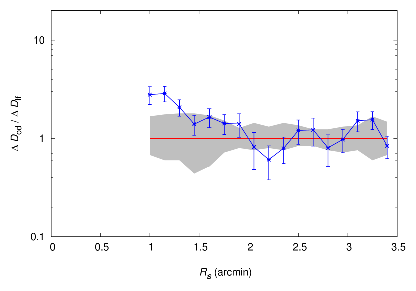
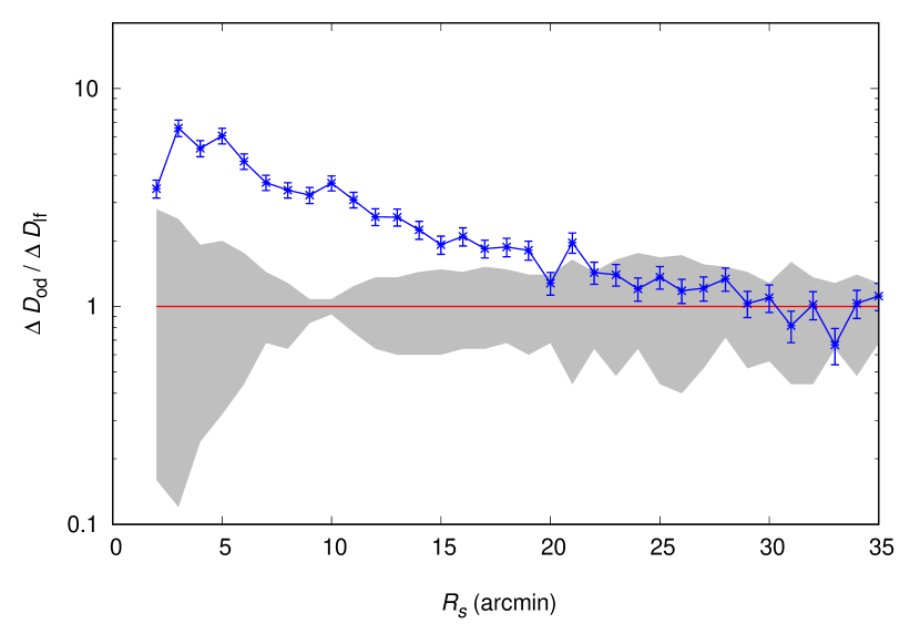
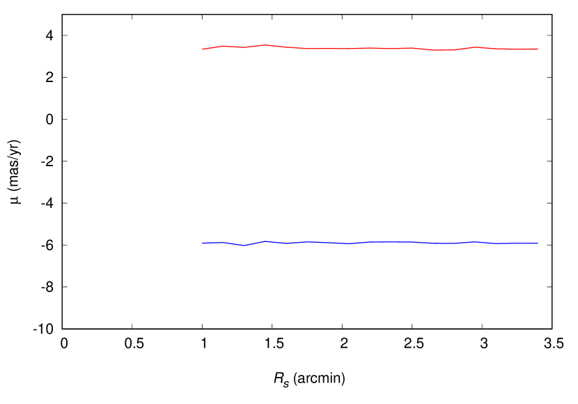
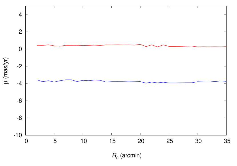
Figure 1: Results of applying the proposed method to the open cluster NGC 3255 (left-hand panel) and NGC 2437 (right-hand panel). Upper panels: blue symbols represent the ratio between density variation in the overdensity region ($\Delta D_{od}$) and density variation in the local field region ($\Delta D_{lf}$) for different sampling radius values ($R_{s}$). Error bars are estimated by assuming Poisson statistics. Red line, shown as reference, corresponds to the case $\Delta D_{od}=\Delta D_{lf}$ expected when $R_{s}$ reaches the actual cluster radius $R_{c}$. Grey area indicates the uncertainty associated to the local field (details in the text). Lower panels: the corresponding overdensity proper motion centroid in right ascension (blue line) and declination (red line) as a function of $R_{s}$.

These two examples correspond to the type A results having the smallest (NGC 3255) and the highest (NGC 2437) found cluster radii. In order to be considered type A, a solution should fulfil two conditions: density changes in the overdensity region should decrease gradually from $\Delta D_{od}>\Delta D_{lf}$ to $\Delta D_{od}\simeq\Delta D_{lf}$, as we can see in upper panels of Figure 1 and, additionally, overdensity centroid in the proper motion space should be unequivocally determined (lower panels). For the open cluster NGC 3255, the first valid sampling occurs at $R_{s}=1$ arcmin and in this case we get $\Delta D_{od}/\Delta D_{lf}\simeq 3$. This means that, as the sampling radius increases, the density of the overdensity increases around three times faster than the local field density. This is because, besides field stars, new cluster stars are being included as $R_{s}$ increases and, therefore, we are still in the $R_{s}<R_{c}$ region in the position space. In spite of fluctuations, the expected general trend toward similar density change values is clearly observed for NGC 3255. Around $R_{s}=1.3$ arcmin blue symbols go into the grey region representing the local field uncertainty and around $R_{s}=2.1$ arcmin they reach the red line corresponding to the $\Delta D_{od}=\Delta D_{lf}$ case. We reflect these uncertainties in the final cluster radius estimation. In the case of NGC 3255, we get $R_{c}=1.3-2.1$ arcmin which is above the value of $1$ arcmin indicated in D02, around the $1.5$ arcmin estimated by Sampedro et al. (2017, hereinafter S17) and clearly below the $\sim 8$ arcmin reported by K13. The highest obtained $R_{c}$ value was for the open cluster NGC 2437 (right panel in Figure 1). The execution of the algorithm for this better sampled cluster clearly starts in the region $R_{s}<R_{c}$ with $\Delta D_{od}\simeq 8\Delta D_{lf}$ and, always with the already mentioned criteria for the lower and upper limits, it returns the solution $R_{c}=22.0-29.0$ arcmin. This range of values is higher than values reported by D02 ($10$ arcmin) and S17 ($17$ arcmin) for this OC but smaller than the one given by K13 ($34$ arcmin).

For both clusters shown in Figure 1, centroids are found always at the same position (see lower panels) which is one of the conditions to be fulfilled in order to be considered a valid solution. Centroid of NGC 3255 is at $(\mu_{\alpha}\cos\delta,\mu_{\delta})=(-5.93,+3.37)$ mas yr^-1 whereas for NGC 2437 is at $(\mu_{\alpha}\cos\delta,\mu_{\delta})=(-3.91,+0.33)$ mas yr^-1. These centroids has been properly found as can be seen in Figures 2, where star proper motion distributions are shown for these two clusters.

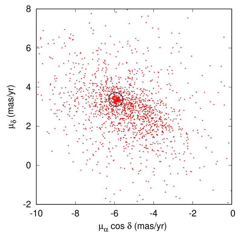
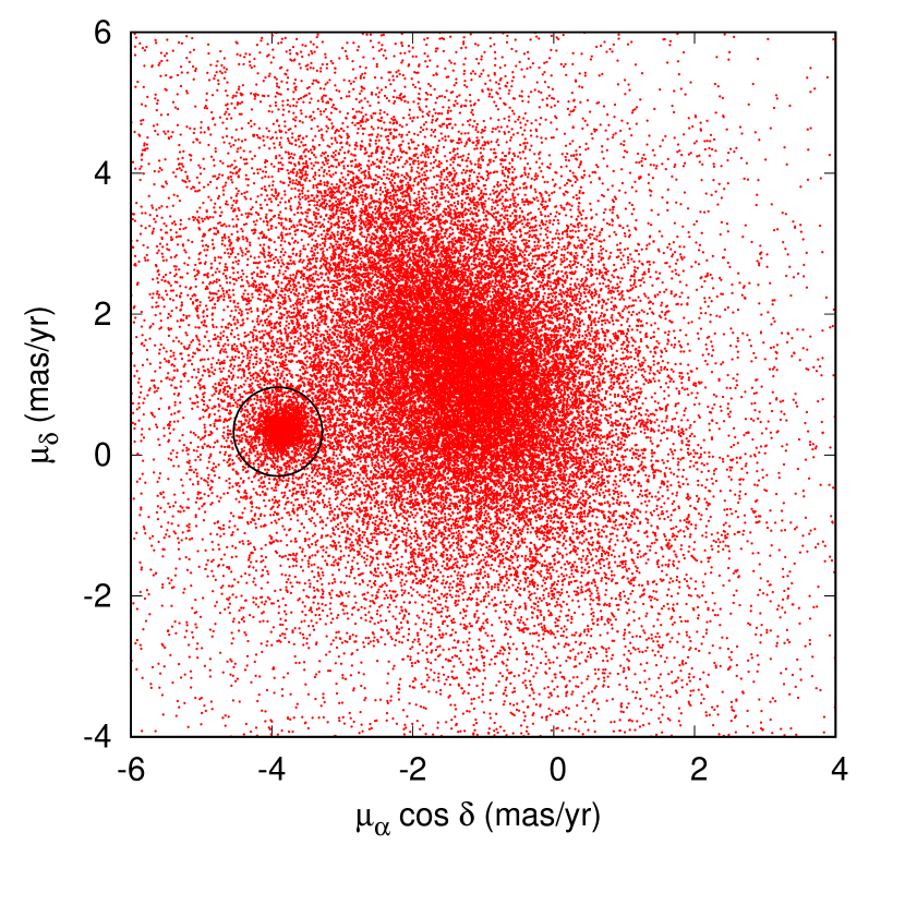
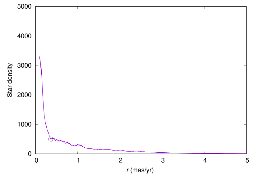
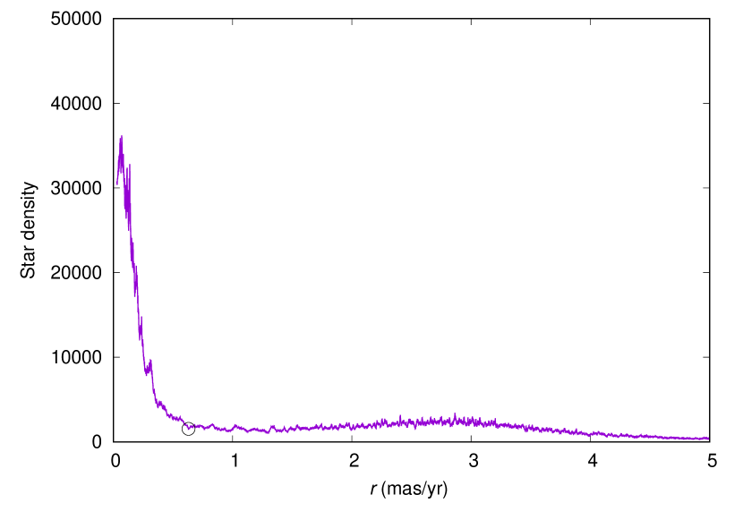
Figure 2: Upper panels: distribution of proper motions for stars in the open cluster NGC 3255 (left panel) y NGC 2437 (right panel) when the sampling radius equals the upper limit of the determined radius: $R_{s}=2.1$ and $R_{s}=29.0$, respectively. Black circles indicate positions and radii of the overdensity determined by the algorithm. Lower panels: the corresponding radial density profiles in stars/(mas/yr)² for the overdensities used to find out their positions and edges (indicated as little open circles over the profiles).

Overdensity “edges" can be clearly seen in the radial density profiles (lower panels in Figures 2) and they are marked with little open circles on the profiles. These points are used as references to estimate overdensity (inside the edges) and local field (outside but close to the edges) densities and their changes at each iteration.

3.2 More uncertain solutions

Some obtained results are not so well behaved as those shown in Figure 1. An example can be seen in left panels of Figure 3, corresponding to the open cluster NGC 2453.

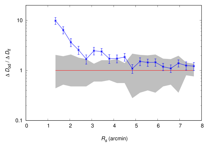
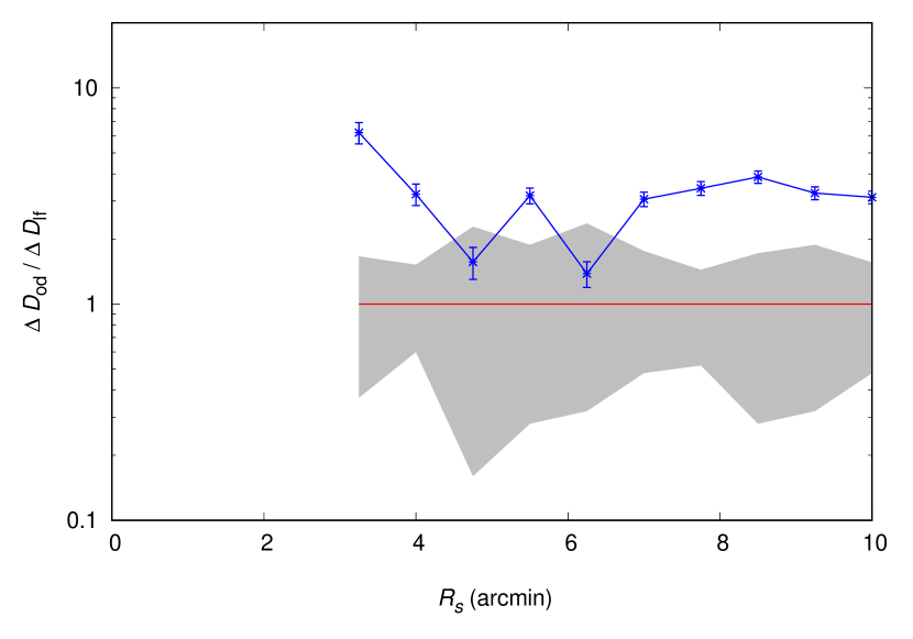
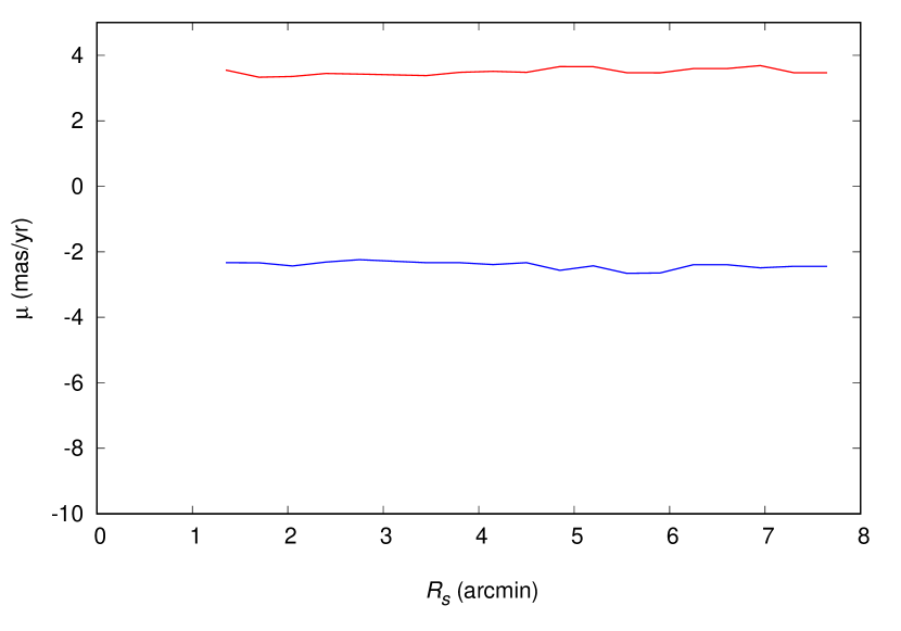
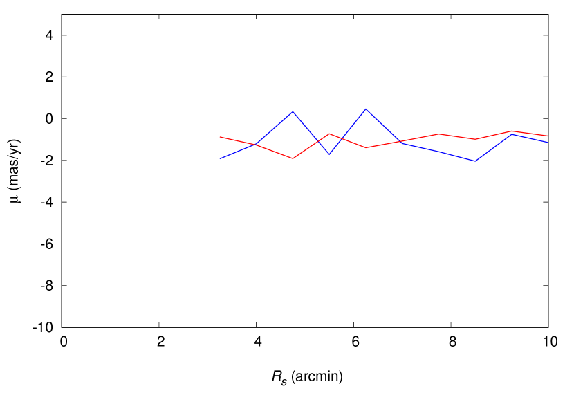
Figure 3: As in Figure 1 but for open cluster NGC 2453 (left panels) and NGC 7801 (right panels).

Even though the algorithm found a suitable and robust cluster centroid in the proper motion space (lower left panel), $\Delta D_{od}/\Delta D_{lf}$ exhibits noticeable fluctuations that make it difficult to clearly constrain lower and upper $R_{c}$ limits. This kind of solutions has been flagged as type B, meaning that we found a valid solution but that $R_{c}$ estimation is more uncertain than in type A solutions. In order to deal with these fluctuations, but maintaining objective criteria, we demand at least two consecutive intersections with grey area or red line for estimating lower and upper radius limits. In any case, all our results were checked by eye to identify type A and B solutions and to confirm that lower and upper radius limits really represent the change from decreasing to nearly constant behaviour in the $\Delta D_{od}/\Delta D_{lf}$–$R_{s}$ plot. With these criteria, we get $R_{c}=4.95\pm 1.35$ arcmin for NGC 2453 (upper right panel in Figure 3). Despite the associated uncertainty, this value is certainly higher than the $2.0-2.5$ arcmin indicated by D02 and S17 but in agreement with the $4.8$ arcmin assigned by K13. A more recent work (González-Díaz et al., 2019) based on Gaia DR2 suggests a higher value, in the range $8-10.5$ arcmin.

3.3 Undetected solutions

We are not reporting results of cluster for which the algorithm did not converge to a valid solution. These cases require further analysis in order to verify whether additional data processing can ensure convergence or, by the contrary, whether there is a physical cause for the non-convergence (for instance a complex proper motion structure or that there is no open cluster at all). Right panels in Figure 3 show the first entry for which we did not find a valid solution corresponding to the open cluster NGC 7801. According to D02 and S17 its radius is $4.0-4.5$ arcmin whereas for K13 it is $9.4$ arcmin. The no-solution is seen in the facts that the result $\Delta D_{od}\simeq\Delta D_{lf}$ is never reached and that the overdensity centroid is not properly found (it is fluctuating in the range $\sim 0-2$ mas/yr). Proper motions of stars in the region of NGC 7801 using $R_{s}=10$ arcmin are shown in Figure 4.

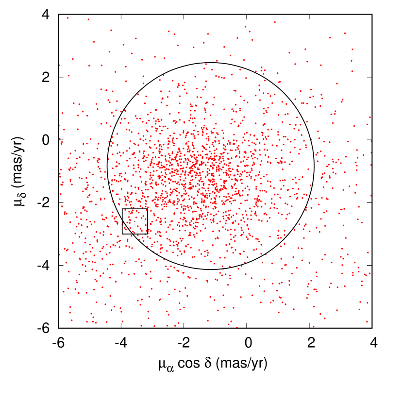
Figure 4: Proper motion distribution of stars in the region of NGC 7801 using a sampling radius of $10$ arcmin. Black circle indicates position and size of the overdensity calculated by the algorithm, that obviously corresponds to the maximum of the field star distribution. Black square indicates, as reference, centroid position according to the D02’s catalogue.

No overdensity is visible by eye in the proper motion space, apart from the maximum of the full distribution, and therefore the algorithm is no able to find a valid solution. The reason is that NGC 7801 is an asterism, as originally suggested by Sulentic & Tifft (1973) and recently confirmed by Cantat-Gaudin & Anders (2020).

There may be different reasons for not finding a valid solution. Firstly, relatively low spatial star densities and/or small angular cluster sizes translate into a first valid $R_{s}$ value above the actual cluster radius. Secondly, there are some cluster catalogued in D02 that does not show (by eye) any clear overdensity in the proper motion space with data from Gaia DR2. These last cases should be analyzed separately in future studies in order to ascertain whether they are star clusters or asterisms (see for example asterisms reported by Cantat-Gaudin & Anders, 2020). There is a third kind of non-valid solution having a recognizable overdensity in proper motion space but that, for some (other) reason, do not reach the condition $\Delta D_{od}\simeq\Delta D_{lf}$ and that will be addressed in future works.

3.4 Catalog of open cluster radii

The application of the proposed method to the sample of OCs listed in D02 has allowed us to build a catalogue with 401 reliable radius values determined in a systematic and independent way through the star proper motions. Main outputs of the algorithm are lower ($R_{low}$) and upper ($R_{opt}$) limits of the cluster radius estimation. According to discussion in Sánchez, Vicente & Alfaro (2010) and Paper I, the upper limit $R_{opt}$ would be the optimal sampling radius needed to be sure of including all cluster stars but minimizing the number of field stars contaminants. In our final catalogue we indicate the estimated cluster radius as a central value $R_{c}=(R_{opt}+R_{low})/2$ and an associated uncertainty $\Delta R_{c}=(R_{opt}-R_{low})/2$. We also report the cluster proper motion $(\mu_{\alpha}\cos\delta,\mu_{\delta})$ estimated for the optimal case $R_{s}=R_{opt}$. Additionally, using the area covered by the overdensity ($A_{od}$), its mean density ($D_{od}$) and also the local field density ($D_{lf}$), we can make an estimation of the number of kinematic cluster member: $N_{c}=(D_{od}-D_{lf})A_{od}$, which will be an upper limit of the actual number of members because additional criteria (for instance parallaxes or photometry) may exclude some stars and because the actual cluster radius may be smaller than $R_{opt}$. The final results are shown in Table 1 and include OC name, equatorial coordinates (J2000), obtained cluster radius ($R_{c}$) and its associated uncertainty ($R_{err}$), a flag indicating type of solution (A or B), the estimated number of kinematic member stars and the mean cluster proper motion.

Table 1: Catalog of cluster radii. This is only a portion for guidance regarding its form and content. The full table is available online.

Name	RA	DEC	$R_{c}$	$R_{err}$	Type	$N_{c}$	$\mu_{\alpha}\cos\delta$	$\mu_{\delta}$
	(deg)	(deg)	(arcmin)	(arcmin)			(mas yr-1)	(mas yr-1)
Berkeley 58	0.05000	60.96667	10.50	2.50	B	357	-3.387	-1.820
Berkeley 59	0.55833	67.41667	6.70	1.90	A	297	-1.608	-2.040
Berkeley 104	0.87500	63.58333	2.75	0.25	A	57	-2.449	+0.129
Berkeley 1	2.40000	60.47500	3.05	0.25	A	76	-2.726	-0.101
King 13	2.52500	61.16667	6.65	2.05	B	534	-2.815	-0.794
Berkeley 60	4.42500	60.93333	3.25	0.25	A	116	-0.629	-0.682
FSR 0486	5.08750	59.31806	2.70	0.50	A	106	+0.119	-0.056
Mayer 1	5.47500	61.75000	4.90	3.30	B	91	-3.213	-1.482
SAI 4	5.91667	62.70389	2.45	0.35	B	319	-2.492	-0.608
Stock 20	6.31250	62.61667	3.60	0.90	A	79	-3.319	-1.235

4 Comparison with other catalogues

4.1 Angular radii

The range of obtained radii goes from $R_{c}=1.4\pm 0.1$ arcmin for the open cluster FSR 1651 (with only $N_{c}=118$ kinematic members) to $R_{c}=25.5\pm 3.5$ arcmin for NGC 2437 ($N_{c}=1891$). It is not a straightforward task to compare our values with those obtained in other studies because the concept of radius is ambiguous itself (it depends on the cluster morphology and structure) and its definition often differs among authors. As mentioned before, we are using the simple, geometric approach in which cluster radius is defined as the radius of the smallest circle containing all assigned members, what we called covering radius in Paper I. Other characteristic radii are the core radius, half-mass (or half-light) radius, tidal radius and the commonly used radial density profile radius, defined as the radius where the cluster surface density drops below field density. Mixing different concepts can lead to inaccurate or biased analysis (see discussions in Madrid, Hurley & Sippel, 2012; Pfalzner, et al., 2016). For example, if most of the OCs follow smooth radial density profiles with very low projected densities in the outer parts, then it is possible that radius values determined from these profiles are systematically below real extents of the clusters (i.e. covering radii as determined here).

The last homogeneous derivation of memberships and OC properties using data from Gaia DR2 was made by C18. They used proper motions and parallaxes to identify members and, from there, to derive very precise properties for a total of 1229 clusters. However, they did not report cluster radii. Their radius $r50$, that containing 50% of the members, is not a reliable description of the total cluster extent. In fact, the first systematic cluster size determination based on Gaia DR2 is presented in this work. We then compare our results with radius values from D02, K13 and S17, which were estimated in different ways. Radii in D02 are just a bibliographic data compilation and, as such, they are heterogeneous with respect to the methods used for estimating them, that include visual inspection. K13 used spatial, kinematic and photometric data from PPMXL (Roeser, Demleitner & Schilbach, 2010) and 2MASS (Skrutskie et al., 2006) to assign memberships and then fitted King’s (King, 1962) profiles to determine cluster radii in a uniform and homogeneous way. From the fitting, K13 obtained the radius for the core (r0), for the central part (r1) and for the cluster (r2). We use the last one for the comparison. On the other hand, Sampedro et al. (2017, hereinafter S17) used star positions given in UCAC4 catalogue (Zacharias et al., 2013) to estimate cluster angular radii through a careful visual inspection of radial density profiles.

In order to compare our results with D02, K13 and S17, we crossmatched the full lists of objects among these catalogues. From the 401 cluster with valid solutions (also included in D02), there are 341 that have radius values reported both in K13 and in S17. Figure 5 compares cluster radius values for these 341 common OCs.

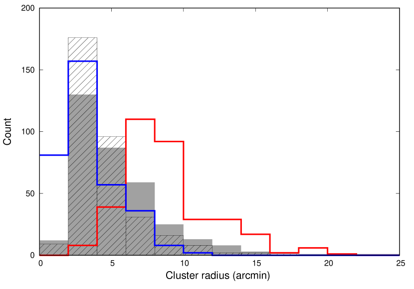
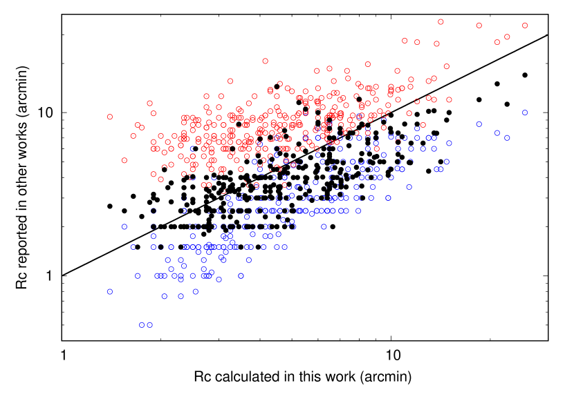
Figure 5: Left panel: Distributions of apparent angular cluster radii estimated in different works: this work (grey bars), D02 (blue line), K13 (red line) and S17 (bars with a diagonal line pattern). Right panel: cluster radii reported in D02 (blue open circles), K13 (red open circles) and S17 (black solid circles) as function of the value estimated in this work. Solid line indicates the 1:1 relation.

We can see clear offsets, being D02’s values consistently smaller and K13’s values consistently larger than our results. Interestingly, there seems to be a good agreement, with no apparent bias, between cluster radii estimated by S17 and our results, each of which is based on different methods and datasets.

4.2 Background-corrected radial density profile

In general, angular sizes obtained with the proposed method agree very well with those reported by S17 (Figure 5), although many particular cases may, of course, differ. S17’s radii were estimated using radial density profiles in the position space. Regardless of the used method, we would expect similar results for the same clusters. For example, for the cluster NGC 2437 (Figure 1) we get $R_{c}=25.5\pm 3.5$ arcmin, clearly above the value $17$ arcmin reported by S17. We have calculated the spatial radial density profile for this cluster with the Gaia DR2 data in the usual way, that is, by counting stars in 2-arcmin width concentric rings around the cluster centre. The profile is shown in Figure 6.

Figure 6: Spatial density profile of stars toward NGC 2437 obtained by using data from the Gaia DR2. Thin black line (corresponding to left y-axis) shows the resulting profile for the full sample of stars and the horizontal dashed line indicates the mean value of $\sim 15.7$ stars/arcmin² calculated in the outermost ring ($30-35$ arcmin). Black thick line (right y-axis using the same units) is an estimation of the actual (clean) cluster density profile by using only stars located inside the proper motion overdensity (see upper right panel in re 1) and removing the estimated proportion of field stars. Vertical bars represent Poissonian statistical errors.

Strictly speaking, density profile (that includes both cluster and field stars) merges into the background at $r=20-22$ arcmin. We have also estimated a background-corrected radial density profile. This was done by using only stars located in the proper motion overdensity region and subtracting the proportion of field star contamination, which is estimated based on the local field-overdensity ratio of densities. The background density was also estimated with the corresponding proportion of field stars. The “clean" profile of spatial density of member stars (black thick line in Figure 6) reaches the zero density level around $\sim 27-29$ arcmin. NGC 2437 radius obtained through spatial density profile is in agreement with the result yielded by our algorithm and the difference with S17’s result seems to be more related to the differences in the used datasets.

4.3 Other outputs

Another algorithm output is the number of estimated kinematic members (number of overdensity stars corrected by subtracting the expected number of field stars). C18 assigned memberships applying an unsupervised algorithm to proper motions and parallaxes from Gaia. Their initial sampling radius were based on D02 and K13 catalogues but they claim that, in principle, membership determination is little affected by the exact sampling as long as the full cluster is sampled (Krone-Martins & Moitinho, 2014). Our number of members ($N_{c}$) correlate very well with C18’s values ($N_{C18}$) in such a way thet the best linear fit passing through the origin is $N_{c}=(1.24\pm 0.02)\cdot N_{C18}$. This means that, on average, we are selecting $\sim$25% more members than C18, something that can be explained by the fact that they included the parallax as an additional discriminant variable and that they restricted their study to stars brighter than $G=18$. Finally, the algorithm also provides cluster proper motions, i.e. centre positions of the overdensities. In Table 2 we compare our results with D02, K13, S17 and C18 for each of the $\sim 300$ clusters in common with these catalogues.

Table 2: Differences between mean proper motions obtained in this work (S20) and those published by D02, K13, S17 (with their three methods: M1, M2 and M3) and C18. Proper motions are in mas yr^-1 and the number following the plus/minus symbol is one standard deviation.

	$\Delta\mu_{\alpha}\cos\delta$	$\Delta\mu_{\delta}$
S20-D02	$-0.23\pm 2.42$	$+0.23\pm 2.49$
S20-K13	$+0.21\pm 2.62$	$-0.02\pm 2.78$
S20-S17(M1)	$-0.57\pm 2.17$	$+0.20\pm 2.46$
S20-S17(M2)	$-0.44\pm 1.95$	$+0.28\pm 2.04$
S20-S17(M3)	$-0.35\pm 2.30$	$+0.54\pm 2.31$
S20-C18	$-0.04\pm 0.50$	$-0.01\pm 0.29$

Generally speaking, our results are consistent with these previous studies with differences, on average, smaller than one standard deviation. As expected, the strongest agreement is with C18 who used data from Gaia. A slight trend is noticeable in which differences with D02 and S17 are opposite to those with K13. It seems that the zero-point differences with UCAC4 and PPMXL catalogues affect more than the different methodologies used in these works.

At this point we have to stress that our method is intended basically to determine OC radii, but the comparison of other derived properties with existing data allow us to check the reliability of our results.

5 Analysis of linear sizes

We have mentioned that angular sizes obtained in this work agree very well with those reported by S17 (Figure 5), even though they were calculated by using different procedures and datasets. When plotted in a log-log plot (upper panel in Figure 7) both distributions follow very similar patterns. Mean radius for both cases is almost the same (around $4.7-4.8$ arcmin).

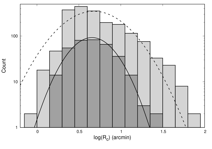
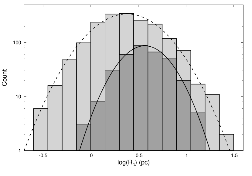
Figure 7: Upper panel: angular size distributions for the full sample of OCs in S17 (light grey bars) and for the subsample with radius values obtained in this work (dark grey bars). Bin size is 0.15 dex. Best fits to lognormal functions are shown as dashed (S17) and solid (this work) lines. Lower panel: the same distributions but for linear radii (in pc) obtained by S17 with distances catalogued in D02 and by us with distances reported by C18.

To analize the linear sizes we cross-matched our results with C18’s catalogue because they determined very precise OC distances from Gaia DR2 parallaxes. Lower panel in Figure 7 shows the result for the 334 clusters in common. We see that the distribution follows very well a lognormal function. This is the kind of distribution that best fit star cluster populations in external galaxies (for instance in M 51 Scheepmaker, et al., 2007). The mean of the distribution is $\log(R_{c})\simeq 0.57$ with a standard deviation $\simeq 0.23$. This characteristic cluster size of $R_{c}\simeq 3.7$ pc is not very different from the value $3.94\pm 0.12$ pc found by Larsen (2004) for the effective radius of OC systems in a sample of $15$ external galaxies observed with the HST. For comparison, we also show in the lower panel of Figure 7 the resulting distribution of S17 using distances from D02. It also follows a well defined lognormal distribution but the mean values differ by 0.2 dex (mean radius in S17 is $\simeq 2.4$ pc). If we only compare distance distributions for 321 cluster that are present in both samples we obtain a very similar difference: our results are practically the same and mean radius in S17 is $\simeq 2.5$ pc. Then, linear sizes estimated in this work are on average 55% higher than the ones in S17. The comparison between the individual distances given by D02 and C18, for our samples, shows very similar values (difference smaller than 7% on average, distances in C18 are higher than those in D02), which is unable to generate the displacement in linear sizes observed in Figure 7 (lower panel). Summarizing, the application of our methodology to a sample of clusters as those listed by S17, but using astrometric data from Gaia DR2, generates a subsample with precise values of angular sizes and any apparent bias, taken individually. However, the comparison between the distributions of angular and linear radii of the S17 catalogue and ours (Figure 7) shows that our most reliable results are obtained for clusters with larger diameters.

5.1 Power-law fitting

Some authors claim that the high-values tail of the radius distribution can be described by a power law of the form $N(R_{c})\sim R_{c}^{\alpha}$, being $N(R_{c})$ the number of objects with radius $R_{c}$ per unit linear size interval. We may expect that young, new-born clusters roughly follow the same distribution of giant molecular clouds, for which on average $\alpha=-3.3\pm 0.3$ (Elmegreen & Falgarone, 1996; Sánchez, Alfaro & Pérez, 2006). It is possible, however, that the star formation process itself and/or the non-uniform early evolution of OCs drastically change or even erase this initial scenario. Bastian, et al. (2005) found a of $\alpha=-2.2\pm 0.2$ for stellar clusters in the disk of the galaxy M 51. For our analysis, we have chosen to fit the number of clusters per unit logarithmic radius interval versus the logarithm of the radius. In such a plot, the power-law tail would be a straightline with slope $\alpha+1$. In addition, we do no set a constant bin size but a constant number of clusters in each bin. It has been proven that this kind of variable sized binning yields bias-free and robust estimates, especially for small sample sizes (Maíz Apellániz & Úbeda, 2005). We carried out several tests varying the minimum radius for the fitting ($3.5$ or $4.0$ pc) and the number of points per bin (between $12$ and $16$), and the slopes obtained were between $-2.03$ and $-2.11$ (with errors between $0.26$ and $0.44$). Figure 8 shows the result for a lower limit of $4.0$ pc and $12$ data points per bin.

Figure 8: Cluster radii distribution (number of clusters per unit logarithmic radius interval). The bin size is such that the number of data points per bin is always $12$. Dashed line corresponds to the best lognormal fitting for the full sample. Solid line stands for the power-law fitting starting from $R_{c}=4$ pc, that yields $\alpha=-3.11\pm 0.35$.

This result is fully compatible with the distribution of molecular clouds ($\alpha\sim-3$). However, it is worth noting that a lognormal function is a much better description for the whole cluster radii distribution (dashe line in Figure 8). Trying to fit a power-law to this kind of distribution is not a suitable approach, although in principle it could be valid when only part of the information (biased toward high radius values) is available.

5.2 $N_{c}$-$T_{c}$-$R_{c}$ relation

Now we proceed to examine the relationship among different variables, in particular number of members ($N_{c}$), cluster radius ($R_{c}$) and age ($T_{c}$). $N_{c}$ is related to the total cluster mass although, in principle, such a connection is not straightforward because we are dealing with a wide range of ages and galactocentric distances, and both dynamical and evolutionary effects may influence the stellar mass function. Relations between the mass (or number of stars), radius and age have been observed for young clusters (see, for example, Pfalzner, 2009; Pfalzner, et al., 2016). Similarly, it has been suggested that Galactic OCs spanning a variety of ages and properties exhibit the same type of scaling relations. There seems to be some correlations between mass, size and age, although there is still considerable uncertainty, especially about the effect of age on the cluster mass or size (see, for example, Schilbach, et al., 2006; Camargo, Bonatto & Bica, 2009; Joshi, et al., 2016; Günes, Karatas & Bonatto, 2017, and references therein). In order to perform this analysis we have adopted cluster ages from Bossini et al. (2019), who used Gaia DR2 astrometric and photometric data to derive precise ages for a sample of 269 OCs, from which we have 63 clusters in common. We constructed a multivariable linear model incorporating the variables $\log N_{c}$, $\log R_{c}$ (pc) and $\log T_{c}$ (Myr), and the best fit to the data yields:

$$N_{c}\propto R_{c}^{1.2\pm 0.1}\cdot T_{c}^{-1.9\pm 0.4}$$

On average, larger OCs have more stars, but additionally younger clusters also tend to contain more stars, i.e. tend to be more massive. This trend agrees with the result obtained by Joshi, et al. (2016) and, in general, with the idea that OCs dissolve slowly with time (Wielen, 1971). Clearly, there are many physical processes acting (simultaneously or at different times) and their mixed effects may spuriously create, amplify, or diminish this kind of relationships.

6 Conclusions

In this work we improve the method proposed in a previous paper (Paper I) for objectively calculating the radius of an open cluster using star positions and proper motions. The method spans the sampling radius around the cluster centre, identifies the cluster overdensity in proper-motion space and compares the changes in star densities between the overdensity and its neighbourhood as the sampling radius increases. The key point of the method is the assumption that these changes should be similar when the sampling radius equals (or is close) to the actual cluster radius. Here we significantly improved the method making it faster than the previous version (Paper I) and much less sensitive to variations of free parameters.

Additionally, we applied the method to all $2167$ open clusters catalogued by D02, using proper motions from the Gaia DR2. From this we obtained a catalogue of $401$ open clusters with reliable radius values calculated with the proposed procedure. On other hand, many of the clusters that did not yield a valid solution do not seem to show an overdensity in proper motions when are seen with data from Gaia DR2 and their true nature should be investigated. The general distribution of angular radii agrees reasonably well with that obtained by S17, whereas some offsets are observed when compared with catalogues of D02 and K13. The obtained distribution of cluster proper motions is consistent with those obtained by D02, K13 and S17, and it is very similar to that reported in C18. Calculated linear sizes follow a lognormal distribution with a mean value of $R_{c}=3.7$ pc, and this distribution shows a shift to higher values with respect to the corresponding S17 distribution. The high radius tail of obtained distribution can be fitted by a power law of the form $N\propto R_{c}^{-3.11\pm 0.35}$. We also found that, on average, younger clusters tend to contain more stars according to the relation $N_{c}\propto R_{c}^{1.2\pm 0.1}\cdot T_{c}^{-1.9\pm 0.4}$, in general agreement with some previous works.

Although the exact behaviour of the algorithm is in some way related to cluster spatial density profile, the proposed method is mainly focused on what happens in proper motions rather than in spatial positions and, therefore, is not sensitive to factors such as low spatial densities or irregular distributions of stars. The only condition of the method to work properly is that the cluster must be visible as an overdensity in the proper motion space. Thus, this method is a good alternative or complement to the standard radial density profile approach.

Appendix A Effect of varying the input parameters

We have carried out several tests to evaluate the performance of the proposed method and to verify that the algorithm does not yield biased results and does not critically depend on input parameters. Tests involved both simulated and real clusters with different characteristics including sizes, number of data points, and overdensity position in the field distribution. In general, the method works well on all cases as long as overdensity is visible in the proper motion space. We have two relevant free parameters already mentioned in Section 2: the minimum number of data points allowed to estimate the density in a given region ($N_{min}$) and the step for spanning the sampling radius ($\delta R_{s}$).

A.1 Parameter $N_{min}$

$N_{min}$ determines, among other things, the sample (bin size) of overdentity profiles (lower panels in Figure 2) making it smoother of noisier. This may affect the exact location of the overdensity “edge". If the overdensity edge determined at a given step is a little closer or further than its “real" position then estimations of overdensity and local field densities will vary. However, the core of the method is to compare density variations as $R_{s}$ increases, and the condition of similar variations ($\Delta D_{od}\simeq\Delta D_{lf}$) when $R_{s}\gtrsim R_{c}$ will be fulfilled independently of the exact edge position. In fact, this condition should be fulfilled in any two relatively small and adjacent regions as long as no new cluster stars are included as $R_{s}$ increases. Therefore, the exact location of the edge has no effect on the final cluster radius obtained.

$N_{min}$ also determines, depending on the projected cluster and field star densities, the minimum starting value for $R_{s}$ (the value corresponding to a sampling large enough). This means that if the cluster radius is smaller than the minimum $R_{s}$ then the algorithm will not find it. In these cases $N_{min}$ should be decreased. After all the tests performed on simulated and real cluster, we have seen that when $N_{min}\lesssim 50$ the density estimations tend to be rather noisy and, therefore, we choose $N_{min}=100$ as the default value used in this work. In any case, final cluster radius values are not substantially affected by the exact value of this parameter. Left panel in Figure 9 compares the $\Delta D_{od}/\Delta D_{lf}$ versus $R_{s}$ plots of the open cluster NGC 2437 for three different $N_{min}$ values.

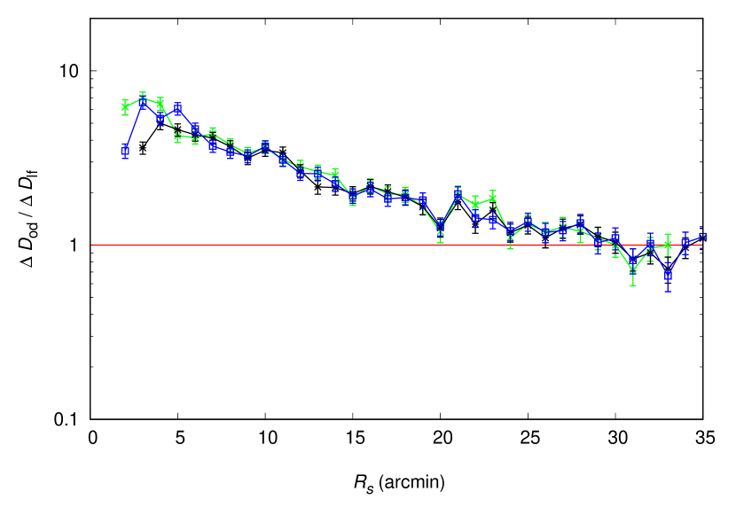
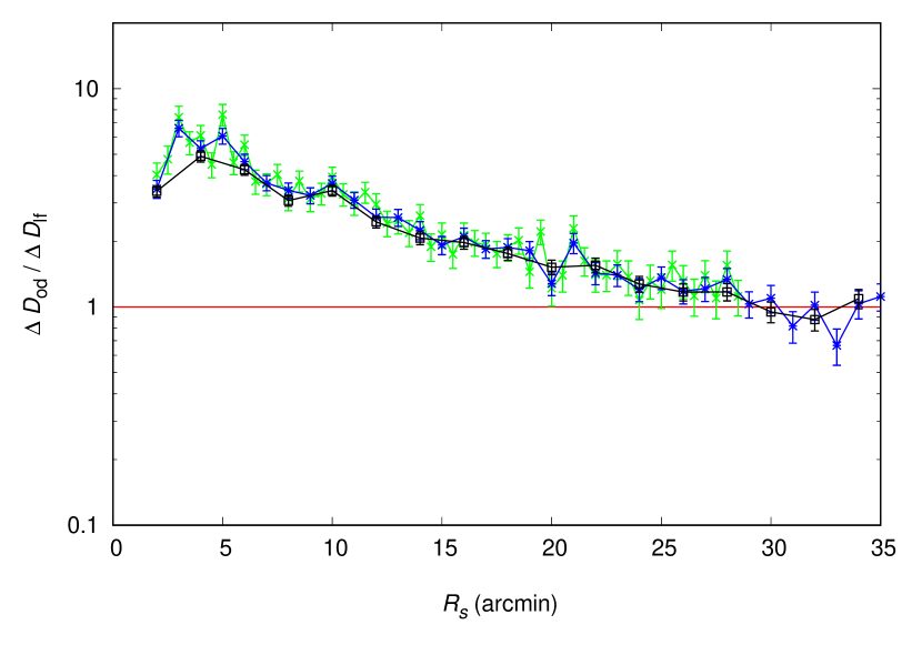
Figure 9: Ratio of density variations ($\Delta D_{od}/\Delta D_{lf}$) of the open cluster NGC 2437 for different values of the free parameters. Left panel: for three values of the minimum number of allowed data points to estimate star densities in a given region: $N_{min}=50$ in green, $N_{min}=100$ in blue and $N_{min}=200$ in black. Right panel: for three values of the step in the sampling radius: $\delta R_{s}=0.5$ arcmin in green, $\delta R_{s}=1.0$ in blue and $\delta R_{s}=2.0$ in black. Uncertainties associated to $D_{lf}$ (grey regions in previous figures) are not shown here for clarity.

The curves are practically the same. For the case $N_{min}=50$ (green line in Figure 9) the obtained cluster radius is $R_{c}=19-29$ arcmin, very similar to the range $R_{c}=22-29$ arcmin obtained for the rest of cases.

A.2 Parameter $\delta R_{s}$

The step size for increasing the sampling ($\delta R_{s}$) is also a free parameter of the algorithm. A relatively small value for this parameter does not necessarily mean a higher precision of the final $R_{c}$ value because, in this case, small changes in the radius imply small increments in the number of new sampled stars and, therefore, higher uncertainties and fluctuations in density change estimations. On the contrary, relatively high $\delta R_{s}$ values imply better density change estimations and produce smoother curves but at the expense of a smaller precision in the obtained $R_{c}$ value. Small or high $\delta R_{s}$ values are relative terms because they depend on the projected spatial density of stars and on the actual cluster radius value (that we cannot know a priori). All the tests performed with the data we are working with (the used list of clusters with proper motions from Gaia DR2) suggested that $\delta R_{s}\sim 1$ arcmin is a good compromise between both extremes and it is chosen as the starting value for the calculation. However, in order to ensure that solution convergence is achieved, the algorithm increases or decreases this initial value depending on the range of $R_{s}$ values to be explored and/or the average density of stars. As with the parameter $N_{min}$, the algorithm behaviour is not greatly affected by the exact value of the step in $R_{s}$. Right panel in Figure 9 compares the results for the cluster NGC 2437 using three different values of this parameter. The algorithm yields noisier or smoother curves but that broadly follow the same pattern as the reference value ($\delta R_{s}=1$) although, obviously, the exact final $R_{c}$ estimation may differ slightly. In this case we get $25.5\pm 3.5$ (for $\delta R_{s}=1$ arcmin), $26.0\pm 4.0$ ($\delta R_{s}=2$ arcmin) and $22.0\pm 2..0$ ($\delta R_{s}=0.5$ arcmin), all compatible inside the error bars.

A.3 Other parameters and conditions

There may be significant differences in proper motion errors between bright and faint sources. However, applying a magnitude cut or filtering by proper motion error does not necessarily improve the results. The reason is that, on the one hand, the quality of the used data becomes better but, on the other hand, the number of data points decreases and this results in more fluctuations in the $\Delta D_{od}/\Delta D_{lf}$–$R_{s}$ plot. In any case, for sufficiently well-sampled OCs we have checked that, although the exact shapes of the curves might differ, the obtained cluster radius remains unaltered (within the calculated uncertainties) when filtering by magnitude or errors in proper motion are applied. This is because the point defining the cluster radius ($R_{s}=R_{c}$, at which no more cluster stars can be added if $R_{s}$ is increased) does not depend on how clearly the overdensity is seen in the proper motion space, as long as it is properly detected.

The exact location of the centre of the cluster is also a relevant issue. We have used cluster positions given by D02 in their catalogue but positions given in other catalogues or actual cluster centres may differ. By using both simulated and well-behaved real clusters, we have verified that, as expected, the shift of the centre of the sampling circle relative to the cluster centre results in an equivalent increase in the obtained cluster radius. Then, if the exact cluster centre is unknown, the $R_{c}$ value obtained with the method proposed in this work should be seen as an upper limit to the actual cluster radius. Generally speaking, we expect this effect to be smaller than the final radius uncertainty. Radius errors for our 401 valid solutions distribute with a mean value of $\sim 1.12$ arcmin (standard deviation $\sim 1.01$ arcmin), whereas angular distances (for the same 401 OCs) between centres reported by D02 (also used by S17) and K13 distribute with a mean of $\sim 0.90$ arcmin (standard deviation $\sim 0.67$ arcmin).

References

- Balaguer-Núñez et al. (2020) Balaguer-Núñez L. et al., 2020, MNRAS, 492, 5811.
- Bastian, et al. (2005) Bastian N., Gieles M., Lamers H. J. G. L. M., Scheepmaker R. A., de Grijs R., 2005, A&A, 431, 905.
- Bica et al. (2019) Bica E., Pavani D. B., Bonatto C. J., Lima E. F., 2019, AJ, 157, 12.
- Bossini et al. (2019) Bossini D. et al., 2019, A&A, 623, A108.
- Cabrera-Cano & Alfaro (1985) Cabrera-Cano J., Alfaro E. J., 1985, A&A, 150, 298.
- Cabrera-Cano & Alfaro (1990) Cabrera-Cano J., Alfaro E. J., 1990, A&A, 235, 94.
- Camargo, Bonatto & Bica (2009) Camargo D., Bonatto C., Bica E., 2009, A&A, 508, 211.
- Cantat-Gaudin et al. (2018) Cantat-Gaudin T. et al., 2018, A&A, 618, A93 (C18).
- Cantat-Gaudin et al. (2019) Cantat-Gaudin T. et al., 2019, A&A, 624, A126.
- Cantat-Gaudin & Anders (2020) Cantat-Gaudin T., Anders F., 2020, A&A, 633, A99.
- Castro-Ginard et al. (2019) Castro-Ginard A., Jordi C., Luri X., Cantat-Gaudin T., Balaguer-Núñez L., 2019, A&A, 627, A35.
- Castro-Ginard et al. (2020) Castro-Ginard A. et al., 2020, arXiv, arXiv:2001.07122.
- Dias et al. (2002) Dias W. S., Alessi B. S., Moitinho A., Lépine J. R. D., 2002, A&A, 389, 871 (D02).
- Dias et al. (2014) Dias W. S., Monteiro H., Caetano T. C., Lépine J. R. D., Assafin M., Oliveira A. F., 2014, A&A, 564, A79.
- Dias, Monteiro & Assafin (2018) Dias W. S., Monteiro H., Assafin M., 2018, MNRAS, 478, 5184.
- Elmegreen & Falgarone (1996) Elmegreen B. G., Falgarone E., 1996, ApJ, 471, 816.
- Ester et al. (1996) Ester M., Kriegel H.-P., Sander J., Xu X., 1996, in Proceedings of the Second International Conference on Knowledge Discovery and Data Mining (KDD-96). AAAI Press, pp 226-231.
- Friel (1995) Friel E. D., 1995, ARA&A, 33, 381.
- Gaia Collaboration et al. (2016) Gaia Collaboration et al., 2016, A&A, 595, A1.
- Gaia Collaboration et al. (2018) Gaia Collaboration et al., 2018, A&A, 616, A1.
- Gieles, et al. (2018) Gieles M., et al., 2018, MNRAS, 478, 2461.
- González-Díaz et al. (2019) González-Díaz D. et al., 2019, A&A, 626, A10.
- Güne\textcommabelows, Karata\textcommabelows & Bonatto (2017) Güne\textcommabelows O., Karata\textcommabelows Y., Bonatto C., 2017, AN, 338, 464.
- Hetem & Gregorio-Hetem (2019) Hetem A., Gregorio-Hetem J., 2019, MNRAS, 490, 2521.
- Joshi, et al. (2016) Joshi Y. C., Dambis A. K., Pandey A. K., Joshi S., 2016, A&A, 593, A116.
- Kharchenko et al. (2012) Kharchenko N. V., Piskunov A. E., Schilbach E., Röser S., Scholz R.-D., 2012, A&A, 543, A156.
- Kharchenko et al. (2013) Kharchenko N. V., Piskunov A. E., Schilbach E., Röser S., Scholz R.-D., 2013, A&A, 558, A53 (K13).
- King (1962) King I., 1962, AJ, 67, 471.
- Kos et al. (2018) Kos J. et al., 2018, MNRAS, 480, 5242.
- Krone-Martins & Moitinho (2014) Krone-Martins A., Moitinho A., 2014, A&A, 561, A57.
- Krumholz, McKee & Bland-Hawthorn (2019) Krumholz M. R., McKee C. F., Bland-Hawthorn J., 2019, ARA&A, 57, 227.
- Larsen (2004) Larsen S. S., 2004, A&A, 416, 537.
- Liu & Pang (2019) Liu L., Pang X., 2019, ApJS, 245, 32.
- Maíz Apellániz & Úbeda (2005) Maíz Apellániz J., Úbeda L., 2005, ApJ, 629, 873.
- Madrid, Hurley & Sippel (2012) Madrid J. P., Hurley J. R., Sippel A. C., 2012, ApJ, 756, 167.
- Netopil, Paunzen & Carraro (2015) Netopil M., Paunzen E., Carraro G., 2015, A&A, 582, A19.
- Ochsenbein, Bauer & Marcout (2000) Ochsenbein F., Bauer P., Marcout J., 2000, A&AS, 143, 23.
- Perren, Vázquez & Piatti (2015) Perren G. I., Vázquez R. A., Piatti A. E., 2015, A&A, 576, A6.
- Pfalzner (2009) Pfalzner S., 2009, A&A, 498, L37.
- Pfalzner, et al. (2016) Pfalzner S., et al., 2016, A&A, 586, A68.
- Randich, Gilmore & Gaia-ESO Consortium (2013) Randich S., Gilmore G., Gaia-ESO Consortium, 2013, Msngr, 154, 47.
- Roeser, Demleitner & Schilbach (2010) Roeser S., Demleitner M., Schilbach E., 2010, AJ, 139, 2440.
- Sampedro & Alfaro (2016) Sampedro L., Alfaro E. J., 2016, MNRAS, 457, 3949.
- Sampedro et al. (2017) Sampedro L., Dias W. S., Alfaro E. J., Monteiro H., Molino A., 2017, MNRAS, 470, 3937 (S17).
- Sánchez, Alfaro & Pérez (2006) Sánchez N., Alfaro E. J., Pérez E., 2006, ApJ, 641, 347.
- Sánchez & Alfaro (2009) Sánchez N., Alfaro E. J., 2009, ApJ, 696, 2086.
- Sánchez, Vicente & Alfaro (2010) Sánchez N., Vicente B., Alfaro E. J., 2010, A&A, 510, A78.
- Sánchez, Alfaro & López-Martínez (2018) Sánchez N., Alfaro E. J., López-Martínez F., 2018, MNRAS, 475, 4122 (Paper I).
- Scheepmaker, et al. (2007) Scheepmaker R. A., Haas M. R., Gieles M., Bastian N., Larsen S. S., Lamers H. J. G. L. M., 2007, A&A, 469, 925.
- Schilbach, et al. (2006) Schilbach E., Kharchenko N. V., Piskunov A. E., Röser S., Scholz R.-D., 2006, A&A, 456, 523.
- Sim et al. (2019) Sim G., Lee S. H., Ann H. B., Kim S., 2019, JKAS, 52, 145.
- Skrutskie et al. (2006) Skrutskie M. F. et al., 2006, AJ, 131, 1163.
- Sulentic & Tifft (1973) Sulentic J. W., Tifft W. G., 1973. The Revised New General Catalogue of Nonstellar Astronomical Objects. Tucson, AZ (USA): University of Arizona Press.
- Vicente, Sánchez & Alfaro (2016) Vicente B., Sánchez N., Alfaro E. J., 2016, MNRAS, 461, 2519.
- Wielen (1971) Wielen R., 1971, A&A, 13, 309.
- Zacharias et al. (2013) Zacharias N., Finch C. T., Girard T. M., Henden A., Bartlett J. L., Monet D. G., Zacharias M. I., 2013, AJ, 145, 44.