Diffusion coefficients in the envelopes of white dwarfs

Abstract

The diffusion of elements is a key process in understanding the unusual surface composition of white dwarfs stars and their spectral evolution. The diffusion coefficients of Paquette et al. (1986) have been widely used to model diffusion in white dwarfs. We perform new calculations of the coefficients of inter-diffusion and ionic thermal diffusion with 1) a more advanced model that uses a recent modification of the calculation of the collision integrals that is more suitable for the partially ionized, partially degenerate and moderately coupled plasma, and 2) classical molecular dynamics. The coefficients are evaluated for silicon and calcium in white dwarf envelopes of hydrogen and helium. A comparison of our results with Paquette et al. shows that the latter systematically underestimates the coefficient of inter-diffusion yet provides reliable estimates for the relatively weakly coupled plasmas found in nearly all types of stars as well as in white dwarfs with hydrogen envelopes. In white dwarfs with cool helium envelopes ($T_{\rm eff}<15000\,$K), the difference grows to more than a factor of two. We also explored the effect of the ionization model used to determine the charges of the ions and found that it can be a substantial source of discrepancy between different calculations. Finally, we consider the relative diffusion time scales of Si and Ca in the context of the pollution of white dwarf photospheres by accreted planetesimals and find factor of $\mathrel{\hbox{\hbox to0.0pt{\lower 2.58334pt\hbox{$\sim$}\hss}\raise 1.72218pt\hbox{$>$}}}3$ differences between calculations based on Paquette et al. and our model.

1 Introduction

White dwarfs (WDs) constitute the end stage of the evolution of the vast majority of stars and are quite common in the Galaxy. With masses of about 0.6 M_⊙ and very small radii of $\sim 10^{9}\,$cm, they have high surface gravities of $\log g\,({\rm cm/s}^{2})\sim 8$ and are characterized by exotic physical conditions such as central densities of up $\sim 10^{6}\,$g/cm³ that are well above those of normal stars and far beyond the reach of current experimental capabilities. On the other hand, WDs are so common that they are very well characterized observationally. They form a fascinating class of stars for the application of theories of dense matter.

In particular, the spectra of WDs indicate that their atmospheric compositions are unlike those of other stars, being composed of pure hydrogen or helium with 25-50% of all WDs showing a small amount of “pollution” from a few heavier elements (Koester et al., 2014). Schatzman (1958) estimated that their high surface gravity would lead to a gravitational settling of the heavier elements by diffusion on time scales of $\sim 10^{6}\,$ years, which explained the nearly pure composition of most WD atmospheres and established the importance of diffusion in WDs. Subsequent studies of the role of diffusion in WD envelopes and atmospheres, combined with other processes such as accretion, convective dredge up, and radiative forces have led to an understanding of the various spectral types of WDs as well as their spectral evolution (see Blouin et al. (2019) for a summary).

The astrophysical interpretation of a large body of WD observations requires a knowledge of the coefficient of inter-diffusion in dense plasmas. This is a challenging endeavor as the plasma can be partially ionized, with partially degenerate electrons, and weakly to strongly coupled ions. Historically, models of diffusion in WDs used coefficients based on the solution of the Bolztmann equation of the kinetic theory of gasses, as obtained by the Chapman and Enskog method (Chapman & Cowling, 1970) or the approach of Burgers (1969). In both approaches, transport coefficients are expressed in terms of binary collision integrals, which is appropriate for dilute gasses (Aller & Chapman, 1960; Michaud, 1970; Michaud et al., 1976; Fontaine & Michaud, 1979; Iben & McDonald, 1985). In low density stellar plasmas, the interaction responsible for the ion collisions can be described as a Coulomb potential with an appropriate choice of long-range cutoff. A considerable advance in physical realism was achieved by Liboff (1959); Mason et al. (1967); Muchmore (1984) and Paquette et al. (1986a) who introduced the static screened Coulomb potential (also called Yukawa or Debye-Hückel) in the collision integrals with a screening length that accounts for electron and ion screening as well as the strong screening limit. The tabulated collisions integrals of Paquette et al. (1986a) have been widely applied in stellar models and to WD models in particular (see, for example, Pelletier et al. (1986); Dupuis et al. (1992); Althaus & Benvenuto (2000); Koester (2009)). A slightly modified physical model has been applied in more recent evaluations of the collision integrals (Fontaine et al., 2015; Stanton & Murillo, 2016).

The last three decades have seen considerable development in the theory of dense plasmas, advanced computer simulation methods, and computational capabilities that justify new calculations of transport coefficients in regimes relevant to WDs. In this paper, we calculate new diffusion coefficients with a more realistic physical model that relaxes several of the key assumptions of Paquette et al. (1986a). Specifically, we present diffusion coefficients of calcium and silicon ions in plasmas of H and He, at the conditions found at the bottom of the superficial convection zone of WDs and compare with the results of Paquette et al. (1986a) and others.

The paper is structured as follows. We first outline in section 2 the three methods that we apply to the calculation of coefficients of diffusion and discuss how they relate to each other as well as their merits and limitations. The details of our calculations of the inter-diffusion and ionic thermal diffusion coefficients are given in Section 3, where we compare the results from various methods. One of the most interesting applications of diffusion in white dwarfs is the combination of accretion and diffusion of metals that explains their presence in the photospheres of DZ and DAZ stars. This process is characterized by the diffusion time scale at the bottom of the convection zone. In section 4 we compare the diffusion time scales of Si and Ca predicted by three models. Section 5 summarizes our work and results and provides a broader perspective on modern calculations of transport coefficients in white dwarf stars.

2 Modeling diffusion coefficients in dense plasmas

In most instances of diffusion in WDs, we are concerned with the inter-diffusion in a binary mixture where one of the species is present as a trace, which is the focus of this paper. For a binary mixture of species with number concentrations $x_{1}$ and $x_{2}$ ($x_{1}+x_{2}=1$), arbitrary electron degeneracy, and in the limit where $x_{2}\ll 1$, the equation for the relative velocity of the species $w_{12}$ due to diffusion is

$$w_{12}=D_{12}\bigg{[} -\frac{\partial\ln x_{2}}{\partial r}+\Big{(}\frac{Z_{2}}{Z_{1}}A_{1}-A_{2}\Big{)}\frac{m_{0}g}{k_{\scriptscriptstyle\rm B}T}$$

$$+\Big{(}\frac{Z_{2}}{Z_{1}}-1\Big{)}\frac{\partial\ln P_{i}}{\partial r}+\alpha_{\scriptscriptstyle T}\frac{\partial\ln T}{\partial r}\bigg{]}$$ (1)

where $D_{12}$ is the coefficient of inter-diffusion, $r$ the radius inside the star, $A_{i}$ and $Z_{i}$ the atomic mass (in a.m.u.) and charge of ions of species $i$ ($i=1$ for the light background ion (H or He) and $i=2$ for the heavy ion), $P_{i}$ the ionic pressure, $T$ the temperature, $k_{\scriptscriptstyle\rm B}$ the Boltzmann constant, $m_{0}$ the atomic mass unit, and $\alpha_{\scriptscriptstyle T}$ is the thermal diffusion factor (Pelletier et al., 1986; Bauer & Bildsten, 2019). The first term on the right hand side of Equation 1 is driven by concentration gradients and corresponds to “ordinary” chemical diffusion. The second and third terms describe barodiffusion, also known as gravitational settling in stars, caused by pressure gradients associated with the star’s gravitational field and the induced electric field. This is generally the dominant term in white dwarf envelopes (Paquette et al., 1986a). The last term is the contribution of thermal diffusion. Equation 1 neglects the contribution of radiative forces which are negligible in the relatively cool white dwarfs we are considering here (Chayer et al., 1995). Furthermore, Equation 1 applies to a single trace ion of charge $Z_{2}$ but in general the trace element has a distribution of charge states, with each ion species described by a separate diffusion equation. An average diffusion velocity for a given element can be defined for such a multi-component diffusion problem but in the following we make the simpler and common approximation of using a single diffusion equation of an element with an average ion charge (Dupuis et al., 1992; Koester, 2009; Bauer & Bildsten, 2019). When $w_{12}>0$ in Equation 1, species 2 moves toward larger $r$ (toward the surface). While Equation 1 is valid for $x_{2}\ll 1$, the calculation of $D_{12}$ is not contingent on that limit. However, the examples presented in section 3 are all for cases where species 2 is a trace. In plasmas, the coefficient of thermal diffusion $D_{\scriptscriptstyle T}=D_{12}\alpha_{\scriptscriptstyle T}$ is determined by collisions between ionic species and between ions and electrons and can be written as $\alpha_{\scriptscriptstyle\rm T}=\alpha_{12}+\alpha_{1e}+\alpha_{2e}$ (Paquette et al., 1986a). In this paper, we consider only the ionic term $\alpha_{12}$. The contributions of $\alpha_{1e}$ and $\alpha_{2e}$ can be comparable or even much larger than $\alpha_{12}$ (Paquette et al., 1986a) and will be the subject of a future publication.

There are several approaches to the calculation of $D_{12}$, three of which are compared here: 1) direct simulation with molecular dynamics, 2) the model of Paquette et al. (1986a), and 3) the effective potential theory which we have developed. We first summarize the main features, advantages and drawbacks of each method.

2.1 Molecular dynamics

Classical molecular dynamics is a simulation method that, when applied to particles such as ions in a plasma, and given an ion-ion pair potential, allows for the direct evaluation of ionic transport coefficients without any assumption beyond those implicit in the input pair potential. Applying the fluctuation-dissipation theorem, it can be shown that the diffusion coefficients $D_{12}$ and $\alpha_{12}$ can be evaluated from a simulation of the system in equilibrium – there is no need to simulate a system with the external gradients that appear in Equation 1. In such a simulation, a large number of classical particles ($\sim 10^{3}$) is set in a cubic box, each with an initial position and a velocity sampled from a Maxwell-Boltzmann distribution. The total force on each particle is summed from the pair interactions with all the other particles. The positions and velocities are advanced in time according to Newton’s second law. An infinite system is approximated by replicating the box in three dimensions with periodic boundary conditions. After a period of equilibration to an imposed value of the temperature, the particles are allowed to move over a relatively long period of time. An analysis of the positions, velocities along the trajectories of the particles can be performed to evaluate many physical properties of interest.

In stellar astrophysics, we are generally concerned with diffusion between two ionic species. The microscopic definition of the coefficient of inter-diffusion between species 1 and 2 is obtained from a time auto-correlation function (Green, 1954; Kubo, 1957; Macquarrie, 1976; Haxhimali et al., 2014)

$$D_{12}=\frac{J}{3Nx_{1}x_{2}}\int_{0}^{\infty}\langle{\bf j}(t)\cdot{\bf j}(0)\rangle\,dt$$ (2)

where

$${\bf j}(t)=x_{2}\sum_{i=1}^{N_{1}}{\bf v}_{1,i}(t)-x_{1}\sum_{i=1}^{N_{2}}{\bf v}_{2,i}(t)$$ (3)

is the net particle current in a system of $N_{j}$ particles of species $j$ of number fraction $x_{j}=N_{j}/N$, and $N=N_{1}+N_{2}$ is the total number of particles. The velocity of particle $i$ of species 1 at time $t$ is ${\bf v}_{1,i}(t)$, which is extracted from the particle trajectories of the simulation. The factor $J$ is the so-called thermodynamic factor

$$J=\frac{x_{1}x_{2}}{k_{\scriptscriptstyle\rm B}T}\frac{\partial\mu_{1}}{\partial x_{1}}\Bigg{|}_{P,T}$$ (4)

where $\mu_{1}$ is the chemical potential of species 1. This factor converts the diffusion coefficient defined in terms of the gradient in the chemical potential (Maxwell-Stefan equation of diffusion) to the coefficient defined in terms of the gradient in the concentration (Fick’s equation of diffusion). In the limit of an ideal gas of neutral particles or for the diffusion of a trace element, $J=1$. The thermodynamic factor can be evaluated from the equation of state (e.g. Equation 4) or, as we have done, from the ionic structure factors $S_{ij}(k)$ of the plasma mixture

$$J^{-1}=x_{2}S_{11}(0)+2\sqrt{x_{1}x_{2}}S_{12}(0)+x_{1}S_{22}(0).$$ (5)

The structure factors $S_{ij}(k)$ are the Fourier transforms of the pair distribution functions $g_{ij}(r)$ that in turn describe the (normalized) radial density profiles of ions of species $j$ around an ion of species $i$. For an ideal gas, ions are spatially uncorrelated and $g_{ij}(r)=1$ but with increasing interactions the ions become correlated, which is reflected in the structure of $g_{ij}(r)$. The evaluation of equation 2 is straightforward from the particle positions produced in a classical MD simulation, although care must be exercised to obtain well-converged results.

The coefficient of ionic thermal diffusivity $D_{\scriptscriptstyle T}=\alpha_{12}D_{12}$ can be evaluated in a similar fashion from classical MD simulations. In this case however, the statistical sampling of the trajectories is much less efficient and the resulting coefficient becomes very noisy. For this reason, we do not present molecular dynamics results for $\alpha_{12}$.

While MD is appealing for its conceptual simplicity and minimal set of assumptions, it does have several numerical drawbacks. Because the system being simulated is relatively small compared to any macroscopic system, it is subject to statistical fluctuations that are particularly significant when evaluating quantities such as $D_{12}$ and $\alpha_{12}$. They can be reduced at the cost of increasing the length of the simulation and the number of particles. As is often the case in WDs, when one species is present as a trace (e.g. $x_{2}\ll 1$) the simulation box contains only a small number of particles of the trace species, greatly increasing the statistical noise in $D_{12}$. Highly asymmetric mixtures, with high mass or charge ratios between the ionic components, are computationally more demanding because of the very different dynamical time scales and interaction forces of the two species (Ticknor et al., 2016). Such mixtures are typical of white dwarfs where the background species is usually H or He and the diffusing species of interest has an atomic number $Z\sim 6-21$. Finally, weakly coupled systems can take a very long time to equilibrate as collisions are weak or infrequent because of low density and energy exchange between particles proceeds slowly. Nonetheless, with current high performance computers, very large and very long MD simulations can be performed to accurately evaluate $D_{12}$ for mixtures (Haxhimali et al., 2014) but this is not practical to generate tables for astrophysical applications.

The values of $D_{12}$ evaluated with classical MD are of course only as reliable as the ion-ion potential that is provided as input to the simulation. In dense plasmas, relatively simple potentials are often used such as a pure Coulomb interaction in the one component plasma and binary ionic mixture models (Hansen, McDonald & Pollock, 1975; Hansen, McDonald & Vieillefosse, 1975; Bastea, 2005; Daligault, 2012; Shaffer et al., 2017), or of a Yukawa form (Salin & Gilles, 2006; Haxhimali et al., 2014). These model potentials represent the limits of a rigid electron background (no screening) and screening in the weakly coupled limit, respectively, and can be accurate in the appropriate physical regimes. As we will see below, realistic self-consistent potentials for dense plasmas can be obtained from an average atom model, without any assumption for its functional form.

The most accurate approaches are quantum MD and orbital free MD that do not require a ion-ion pair potential. Instead, the simulation considers only classical nuclei and quantum electrons and almost always in the Born-Oppenheimer approximation where the kinetic degrees of freedom of the electrons are decoupled from those of the ions. The density of the quantum electron fluid in the simulation box is calculated by solving the Schrödinger equation or the Thomas-Fermi model, respectively, for each configuration of the nuclei at each time step. The force on each nucleus is the sum of the forces from all the other nuclei and from the 3-dimensional density of the electron fluid. Unfortunately, these methods are computationally very intensive, which severely limits the size and length of the simulations, but have nevertheless been applied to the computation of the self- and inter-diffusion coefficients (Lambert, Clérouin & Mazevet, 2006; Kress et al., 2011; Danel, Kazandjian & Zérah, 2012; Rudd et al., 2012; French et al., 2012; Jakse & Pasturel, 2013; Burakovzky et al., 2013; Meyer et al., 2015; Sjostrom & Daligault, 2015; Ticknor et al., 2015). Here, we use classical MD simulations to evaluate coefficients of inter-diffusion for the purpose of validating the results obtained with the Paquette et al. (1986a) model and the effective potential theory method that we have developed.

2.2 Introduction to the kinetic theories of Paquette et al. and Effective Potential Theory

A goal of kinetic theory is to express as accurately as possible formal relations such as Equation 2 explicitly in terms of the interaction potentials between particles and in a form that makes their numerical evaluation straightforward in comparison with molecular dynamics simulations. Models of this kind for the coefficient of ionic inter-diffusion in stars are based on the expression derived from the solution of the Boltzmann kinetic equation (Burgers, 1969; Chapman & Cowling, 1970). The resulting transport coefficients are expressed in terms of collision integrals involving scattering cross sections for isolated, binary collisions. The application of this approach to plasmas is not straightforward. Indeed, strictly speaking, the Boltzmann equation is only valid for gases of particles with short-range binary interactions that are dilute enough that the particle dynamics can be described as a succession of spatially localized and uncorrelated binary encounters. This approximation does not directly apply to a plasma regardless of its density or its temperature, because the long-range nature of the Coulomb potential invalidates the assumption of spatially localized collisions and, as a consequence, leads to divergent collision integrals. Yet, the difficulty can be remedied by considering that in a plasma, two charged particles never interact directly via the Coulomb potential because the presence of the surrounding particles screens the interaction, resulting in an effective binary interaction potential that is short-ranged. When the latter is used in the Boltzmann equation in place of the bare Coulomb potential, the resulting transport coefficients remain finite. The simplest form of effective interaction is a pure Coulomb potential with a long-range cutoff, usually chosen as the Debye screening length (Equation 8). In accordance with Boltzmann’s theory, the effective potential approach is appropriate if the dynamics of charged particles can be described as a succession of binary collisions in this effective potential. This is the case in weakly coupled plasmas, i.e. under density and temperature conditions that are such that the typical kinetic energies of particles is much larger than their typical mutual interactions. Interestingly, in WD plasmas, electrons are generally weakly coupled to other electrons and to ions either because of the high temperature or the high quantum degeneracy. Conversely, the ions typically remain non-degenerate and can become strongly coupled at low enough temperature.

The two kinetic theories used in this work, namely the model of Paquette et al. and the more advanced effective potential theory, rest upon two different models of the effective ion-ion potential designed to give accurate transport coefficients in the weak and the moderately coupled plasma regimes, respectively. The Paquette et al. approach assumes that the effective pair interaction is a screened Coulomb potential, which accounts for screening by both electrons and ions in the weakly coupled limit. More generally, Baalrud & Daligault (2019) have shown that the postulate of an effective pair interaction in the Boltzmann equation can be rigorously derived from a kinetic theory based on an expansion in terms of the departure of correlations from their equilibrium values. The derivation also yields the proper form of the potential in the Effective Potential Theory, which we apply in this study.

2.3 Model of Paquette et al. (1986)

The strength of the coupling between two ions of charge $Z_{1}$ and $Z_{2}$ is conveniently quantified by the coupling parameter

$$\Gamma=\frac{Z_{1}Z_{2}e^{2}}{ak_{\scriptscriptstyle\rm B}T}\,,$$ (6)

which is the ratio of the Coulomb energy between two neighboring ions to their kinetic energy, $a$ being the ion sphere radius, and $e$ the (positive) quantum of charge. Ions are weakly coupled when $\Gamma\ll 1$. In weakly coupled plasmas, the linear response approximation can be used to determine the effective interaction between two ions (Eliezer et al., 2002). This yields the static screened Coulomb potential

$$V_{\scriptscriptstyle\rm D}(r)=\frac{Z_{1}Z_{2}e^{2}}{r}e^{-r/\lambda_{\scriptscriptstyle D}}$$ (7)

where

$$\lambda_{\scriptscriptstyle D}=\bigg{[}\lambda_{i}^{-2}+\lambda_{e}^{-2}\bigg{]}^{-1/2}$$ (8)

is the total screening length that accounts for the screening of the ion interactions by both ions and electrons, with $\lambda_{i}^{2}=k_{\scriptscriptstyle\rm B}T/4\pi e^{2}\sum_{i}{n_{i}Z_{i}^{2}}$ the classical Debye-Hückel screening length of ions and $\lambda_{e}$ the electron screening length. The regime of validity of this approach can be extended to $\Gamma\sim 0.3$. Beyond, the weak coupling approximation fails and the screening is no longer described by Equation 8. It was suggested on physical grounds that an approximate potential that extends the domain of validity of the screened potential (7) is obtained by replacing the screening length by the ion sphere radius $a$. Thus the weak coupling limit and an approximation of the strong coupling limit can be obtained by choosing a screening length

$$\lambda=\max\{\lambda_{\scriptscriptstyle D},a\}.$$ (9)

Muchmore (1984), Paquette et al. (1986a), and Brassard & Fontaine (2014) used the potential defined by Equations (7–9) to evaluate the coefficients of inter-diffusion and thermal diffusion, using the classical limit for the electron screening length $\lambda_{e}^{2}=k_{\scriptscriptstyle\rm B}T/4\pi e^{2}n_{e}$. Recently, Fontaine et al. (2015) and Stanton & Murillo (2016) revised the work of Paquette et al. (1986a) by using the Thomas-Fermi screening length for the electrons to account for electron degeneracy

$$\lambda_{\scriptscriptstyle\rm TF}^{2}=2\frac{I_{1/2}(\beta\mu_{\rm e})}{I_{-1/2}(\beta\mu_{\rm e})}\lambda_{e}^{2},$$ (10)

where $\beta=1/k_{\scriptscriptstyle\rm B}T$, $\mu_{\rm e}$ is the chemical potential of the electrons and

$$I_{n}(\alpha)=\int_{0}^{\infty}\frac{x^{n}}{e^{x-\alpha}+1}\,dx$$ (11)

is the Fermi integral of index $n$. Equation 10 reduces to the classical Debye-Hückel length in the non-degenerate limit. Both of these works also implemented a smoother transition to the strongly coupled approximation by replacing Equation 9 with

$$\lambda=\frac{\lambda_{\scriptscriptstyle\rm D}^{5}+a^{5}}{\lambda_{\scriptscriptstyle\rm D}^{4}+a^{4}}$$ (12)

(Fontaine et al., 2015) while Stanton & Murillo (2016) chose a more physically motivated interpolation form

$$\lambda=\Bigg{(}\frac{1}{\lambda_{\scriptscriptstyle\rm TF}^{2}}+\frac{1}{\lambda_{i}^{2}+a^{2}}\Bigg{)}^{-1/2}.$$ (13)

The collision integrals involving the static screened potential must be evaluated numerically. However, a considerable advantage of this approach is that they can be expressed in dimensionless form with the parameters of the specific mixture (masses and charges of the ions) factored out (Paquette et al., 1986a). Thus, the dimensionless collision integrals for the static screened potential can be evaluated once and for all for any mixture. On the other hand, for dimensional calculations of diffusion coefficients, a separate model is needed to provide the charges of the ions $Z_{i}$ that enter the pair potential. The simplest approach is to estimate the ion charge with the Thomas-Fermi average atom model (Stanton & Murillo, 2016). The choice of ionization model is a source of uncertainty in the calculated values of $D_{12}$ (Bauer & Bildsten, 2019) and transport coefficients in general (Grabowski et al., 2020). We will return to this point in section 3.

Since their publication, the fits of the collision integrals of Paquette et al. (1986a) have been used in nearly all models of diffusion in white dwarfs stars, and in numerous calculations of diffusion in stars in general. Because of their prevalence in stellar astrophysics, they represent a standard for comparison with our own calculations of $D_{12}$ and $\alpha_{12}$.

2.4 Effective Potential Theory

The effective potential theory (EPT, Baalrud & Daligault (2013, 2015)) extends the range of validity of the Boltzmann equation and the associated Chapman-Enskog solution for ionic transport coefficients to strong ion coupling by rigorously including their correlations in the pair potential. This accounts for the presence of the surrounding ions in a collision between two ions. This was recently derived from first principles (Baalrud & Daligault, 2019) with an expansion in terms of the departure of correlations from their equilibrium values rather than in terms of the strength of the correlations. This gives a kinetic equation that is similar to the Boltzmann equation but in which the pair potential $V_{ij}(r)$ is replaced by the potential of mean force, $V_{ij}^{\rm eff}(r)$. By definition, the potential of mean force is related to the pair distribution function

$$g_{ij}(r)=\exp(-V^{\rm eff}_{ij}(r)/k_{\scriptscriptstyle\rm B}T).$$ (14)

Given a pair interaction potential $V_{ij}(r)$, the pair distribution function can be extracted from classical MD simulations, or more economically with the integral theory of fluids (Hansen & McDonald (2013), Chap. 4). Inverting Equation (14) gives $V^{\rm eff}_{ij}(r)$, which is then applied in the Chapman-Enskog collision integrals. In the limit of a weakly coupled system, $V^{\rm eff}_{ij}(r)\rightarrow V_{{\scriptscriptstyle\rm D},ij}(r)$, the static screened Coulomb potential (Equation 7), and the dilute gas limit is recovered exactly. The EPT has been extended to mixtures (Beznogov & Yakovlev, 2014; Daligault et al., 2016; Shaffer et al., 2017). Since the EPT can be solved for transport coefficients using the Chapman-Enskog formalism, the evaluation of the diffusion coefficient is very fast. It gives self-diffusion coefficients with an accuracy better than 9% for $\Gamma<30$ for the one-component plasma (Baalrud & Daligault, 2015), and matches ab initio simulations of a deuterium plasma to better than 6% where $\Gamma\leq 9.5$ (Daligault et al., 2016). In general, the potential of mean force $V^{\rm eff}_{ij}(r)$ must be evaluated numerically even for a pair potential $V_{ij}(r)$ with a simple analytic form. The practical advantage of the single pre-tabulation of the Paquette et al. collision integrals for any binary mixture of ions is lost with the EPT.

The EPT theory is general and can be applied to systems interacting with any pair potential, as long as $g_{ij}(r)$ is known. The most reliable $g_{ij}(r)$ come from ab initio simulations but then little is gained in terms of computational cost. Instead, we use a recently developed model for dense plasmas that combines an average atom model with the integral theory of fluids that provides both a pair potential and the corresponding radial distribution function.

2.4.1 Model for the ion-ion potential in dense, partially ionized plasmas

In view of the computational cost of quantum MD simulations and the severe limitations of heuristic models of pressure ionization, we have adopted a recently developed model of dense, partially ionized, partially degenerate, and weakly to strongly coupled plasmas that combines both physical realism and relative ease of computation. The average-atom, two-component plasma model (AA-TCP) considers a plasma composed of identical ions with an average charge ${\bar{Z}}$ with bound electrons in a sea of quantum mechanical electrons of arbitrary degeneracy. The model has no adjustable parameters and only requires the composition, temperature and density of the plasma as inputs. It provides a self-consistent solution for the energies and wave functions of the bound and continuum states, the average ion charge, all correlation functions in the fluid, and the ion-ion pair potential. It naturally accounts for strongly non-linear screening as well as pressure and temperature ionization and it can treat arbitrary mixtures without any additional approximation (Starrett & Saumon, 2013a, b, 2014a, 2014b). The pair potential does not have a prescribed functional form such as the Yukawa potential but is calculated numerically within the model. The AA-TCP ion-ion potential $V_{ij}(r)$ can be used as an input to classical MD simulations, resulting in a dense plasma model called Pseudo-Atom Molecular Dynamics (PAMD, Starrett et al. (2015a)), or in the EPT model through the corresponding $g_{ij}(r)$ (Daligault et al., 2016). A limitation of this model is that it does not account for a distribution of ionic charge states. All ions of a given species have the same average charge.

The AA-TCP model is based on well-established theory but its formulation and numerical implementation are fairly elaborate. The model was developed and has evolved over several years. A recent review (Saumon & Starrett, 2020) provides a guide to the key publications. A more pedagogical introduction to the concepts and elements of such models is given in Saumon et al. (2014). Starrett & Saumon (2014a) summarizes the final version of the model for a plasma with one ion species and includes a discussion of several key numerical details.

The AA-TCP model has been validated by numerous comparisons with ab initio simulations and generally gives excellent results for the pair distribution function – a test of the quality of $V_{ij}(r)$ – (Starrett & Saumon, 2013a, b, 2014a, 2014b), the equation of state (Starrett & Saumon, 2016) and diffusion coefficients (Daligault et al., 2016) over a wide range of temperatures and densities for elements ranging from hydrogen to tungsten, including binary mixtures. It also compares very well with an accurate X-ray Thomson scattering experiment on warm dense aluminum (Starrett & Saumon, 2015b). The combination of the AA-TCP model with the EPT thus opens the possibility of computing inter-diffusion coefficients with a high degree of physical realism at a reasonable computational cost. While the combination of the EPT and AA-TCP models is more approximate than ab initio simulations in strongly coupled plasmas, it can handle systems with trace species and highly asymmetric mixtures without difficulty and is considerably more economical.

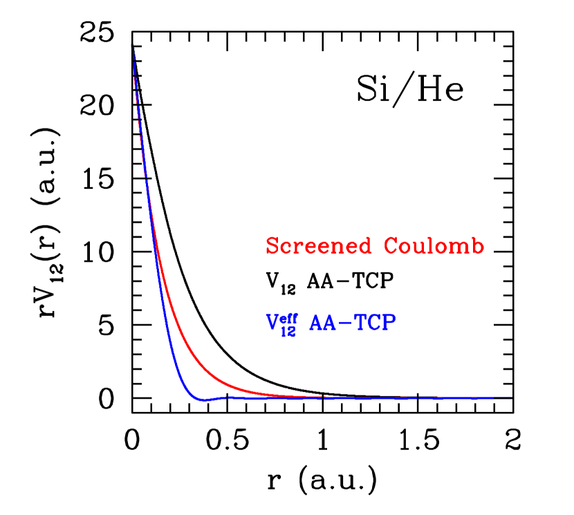
Figure 1: Comparison of Si-He pair potentials used in three different approaches to compute diffusion coefficients. The plasma is a mixture of He with a trace of Si ($x({\rm Si})=10^{-3}$) at $\log T\,({\rm K})=5.737$, $\log\rho\,({\rm g/cm}^{3})=3.486$ (see Table 3). The average ion charges, obtained with the AA-TCP model, are ${\bar{Z}}({\rm He})=Z_{1}=2.000$ and ${\bar{Z}}({\rm Si})=Z_{2}=12.121$ for all three potentials. This plasma is strongly coupled ($\Gamma=15.259$) and strongly degenerate ($k_{\scriptscriptstyle\rm B}T/\epsilon_{\scriptscriptstyle\rm F}=0.014$). For clarity, the product $rV_{12}(r)$ is shown so that as $r\rightarrow 0$, $rV_{12}(r)=Z_{1}Z_{2}$. Under these conditions, the screened Coulomb potential (Equations 7–13) has reached the limit where the screening length $\lambda=a=0.152\,$ a.u. regardless of whether one uses the definition of Paquette et al. (1986a), Fontaine et al. (2015) or Stanton & Murillo (2016). Those three screened Coulomb potentials are thus identical here. $V_{12}$ is the ion-ion pair potential from the AA-TCP model and $V_{12}^{\rm eff}$ is the corresponding potential of mean force (Equation 14). [See the electronic edition of the Journal for a color version of this figure.]

2.4.2 Comparison of ion-ion potentials

A comparison of the ion-ion potentials used in the above models illuminates how each accounts for the physics of correlations and screening in the plasma. For this purpose, we choose plasma conditions that emphasize the differences between the potentials and for which the diffusion coefficients vary significantly (see section 3). Figure 1 shows potentials for a plasma of He (species 1) with a trace of Si (species 2, $x_{2}=10^{-3}$) at the bottom of the convection zone of a low-$T_{\rm eff}$ white dwarf with a He envelope ($\log T\,({\rm K})=5.737$ and $\log\rho\,({\rm g/cm}^{3})=3.486$). Under those conditions, the average ion charges obtained with the AA-TCP plasma model are ${\bar{Z}}({\rm He})=2.000$ and ${\bar{Z}}({\rm Si})=12.121$. For the purpose of this comparison, these values are applied to the calculation of all three potentials shown. The coefficient of inter-diffusion of Si in a He-dominated plasma is determined by the Si-He pair potential while the plasma conditions (electron density and degeneracy) are dominated by the background He plasma. The figure shows the product $rV_{12}(r)$ for clarity, giving a finite and common value of $Z_{1}Z_{2}=24.242$ at $r=0$. A pure Coulomb potential would appear as a horizontal line. The rapid decrease of $rV_{12}(r)$ away from the origin reflects the screening of the pure Coulomb interaction by electrons and ions. The Si-He pair potential $V_{12}(r)$ from the AA-TCP model in Figure 1 accounts for electron screening only. In this case the screening is from the cloud of free electrons surrounding each ion (He and Si) obtained by solving the Schrödinger equation for free states including the interactions with other electrons and the surrounding ions. This potential can describe the highly non-linear screening by free electrons in plasmas with strong electron-electron and electron-ion couplings, as well as the inherently non-linear bound states. The AA-TCP pair potential is used in the classical molecular dynamics simulations (PAMD) that simulate the ion-ion correlations (i.e. ion screening) to all orders. Both electron and ion screening are included in the screened Coulomb potential (Equations 7 and 8) but in the linear limit of weak coupling. For dense, strongly coupled plasmas, the screening length is made to approach the ion sphere radius (Equations 9, 12, 13), which mimics the effect of strong ion screening and corrects the failure of the weakly screened Coulomb potential. This strong screening limit is reached in this particular example and all three choices of the screening length revert to the ion sphere radius and all three potentials are identical (given that they all use the same ion charges). In this approximate description, the introduction of ion correlations softens the pair potential significantly compared to the AA-TCP pair potential. Finally, the effective potential $V_{12}^{\rm eff}(r)$ (Equation 14) is the potential of mean force built from the AA-TCP pair potential $V_{12}(r)$ that accounts for electron screening and the pair distribution function that accounts for ion screening. This is the potential used in the EPT of transport coefficients and is the least repulsive of all three. This comparison shows that the simple modifications of the screening length of Paquette et al. (1986a), Fontaine et al. (2015) and Stanton & Murillo (2016) do not properly account for strong ion screening except at very short range ($r\mathrel{\hbox{\hbox to0.0pt{\lower 2.58334pt\hbox{$\sim$}\hss}\raise 1.72218pt\hbox{$<$}}}0.1\,$a.u.). In general a more repulsive potential results in a larger collisional cross-section and, as we will see below, smaller diffusion coefficients.

Table 1: Comparison of the approximations in the models used to calculate diffusion coefficients herein

Quantity	Paquette et al.	Molecular Dynamics (PAMD)	Effective Potential Theory
Ion charge	From a separate model	Implicit in input $V_{ij}(r)$	Implicit in input $g_{ij}(r)$
		from AA-TCP model	from AA-TCP model
Ion-ion pair potential	Static screened Coulomb	From AA-TCP model	Implicit in input $g_{ij}(r)$
	“Yukawa”		from AA-TCP model
Order of the collisions	2-body	N-body	2-body and higher order
Diffusion coefficients	Collision integrals	From particle	Collision integrals with
	with Yukawa $V_{ij}(r)$	trajectories	effective $V_{ij}^{\rm eff}(r)$
Thermodynamic factor	$J=1$	From AA-TCP model	Non-ideal
			(within EPT approximation)

2.4.3 Summary of methods

To summarize, there is a hierarchy of models and approximations that allow the computation of diffusion coefficients in white dwarf atmospheres. In order of increasing physical sophistication and also of computational cost, the models discussed here are 1) the Chapman-Enskog theory of transport in dilute gases with collision integrals for Coulomb potentials with an appropriate radial cutoff, 2) the Paquette et al. (1986a) approach that uses the same formalism but with a static screened Coulomb potential, 3) the EPT theory that extends the Chapman-Enskog formalism to strongly coupled plasmas by including ion correlations in the pair potential, 4) classical molecular dynamics, and 5) ab initio molecular dynamics. The EPT can be applied to any pair potential such as pure Coulomb, Yukawa and more sophisticated potentials. The first three approaches can all be used from the very weak coupling limit up to various degrees of coupling, and have low computational costs. Classical MD can be used with any repulsive potential and has no physical approximation other than those implicit in the potential but is much more costly. It works well in the moderate to very strong coupling regime. We use classical MD below to validate the EPT results. The ab initio methods are based on classical MD for the ions but rather than using a prescribed ion-ion potential, they use a model for calculating the structure of the electron fluid in the three-dimensional simulation box and the resulting forces on the ions. They are thus much more expensive. The simplest form of ab initio simulation that treats the electrons explicitly is the Thomas-Fermi orbital free MD which is suitable for hot and dense plasmas. Finally, the most accurate and most expensive method is quantum MD, where the electrons are modeled quantum mechanically. For computational reasons it is limited to rather low temperatures, typically $\lesssim 10^{5}\,$K. The main features of the three models we apply here are summarized in Table 1.

Computationally, the evaluation of the diffusion coefficients of Paquette et al. (1986a) and Stanton & Murillo (2016) are very fast as they require only the evaluation of a fit to pre-evaluated collision integrals for the analytic screened Coulomb potential. The EPT is slower because it evaluates the collision integrals using the potential of mean force which is not pre-determined but this is relatively fast, given a potential. In both cases, however, a model of the equation of state must be run to obtain the ion charges and/or the potential, which is far more costly than the evaluation of the collision integrals. The AA-TCP model is a reliable and advanced model for dense, partially ionized plasmas but its evaluation can take a few minutes to an hour per $(\rho,T)$ point, depending on the conditions and the atomic number of the elements in the mixture. For practical applications, diffusion coefficients evaluated with the combination of the AA-TCP model and of the EPT must be pre-tabulated for the specific mixture. Finally, ab initio methods typically take 2 orders of magnitude longer than the AA-TCP model for evaluating the equation of state/potential and even longer to obtain diffusion coefficients.

3 Coefficients of inter-diffusion and ionic thermal diffusion

Our main purpose is to revisit the calculation of diffusion coefficients under the conditions found in white dwarf envelopes with the EPT using AA-TCP potentials and compare with the values from the more approximate model of Paquette et al. (1986a). We also present a validation of the EPT results against classical MD results that use the same ion-ion potential $V_{ij}(r)$ that gives $V_{ij}^{\rm eff}(r)$ for the EPT calculation. This tests the accuracy of the EPT but not that of the input potential that must be validated separately.

Cool white dwarfs develop a surface convection zone where the mixing time scale is much shorter than the diffusion time, resulting in a homogeneous composition throughout the convective region. In the simplest picture, the abundances of heavy elements in the convection zone (which are observable in the star’s spectrum) decrease as those ions diffuse below the bottom of the convection zone. Thus we focus on diffusion at the bottom of the convection zone as the most relevant regime for the spectral evolution of white dwarf stars.

We calculate the coefficient of inter-diffusion $D_{12}$ and the ionic contribution $\alpha_{12}$ to the thermal diffusion factor $\alpha_{\scriptscriptstyle T}$ (Equation 1) in white dwarf models with both pure hydrogen and pure helium envelopes. We consider the diffusion of traces of silicon and calcium which are two well-observed elements in the spectra of metal-polluted WDs (Zeidler-K. T. et al., 1986; Dupuis et al., 1993; Dufour et al., 2007). The properties of the convection zone are taken from selected models along two white dwarf cooling sequences with a mass of $M_{\star}=0.6\,$M_⊙, a pure carbon core, a He layer with a mass fraction of $10^{-2}\,M_{\star}$ and, for the H case, a superficial hydrogen layer with a mass of $10^{-4}\,M_{\star}$. The convection is modeled with the ML2 parametrization of the mixing length theory. These evolution models are described in Fontaine, Brassard & Bergeron (2001). For each model in a sequence, the effective temperature, radius, gravity, temperature and density at the bottom of the convection zone, and fractional mass of the convection zone are given in Tables 2 (H case) and 3 (He case). The last two columns give the values of two important plasma parameters, the electron degeneracy parameter $k_{\scriptscriptstyle\rm B}T/\epsilon_{\scriptscriptstyle F}$, where $\epsilon_{\scriptscriptstyle F}$ is the Fermi energy, and the plasma coupling parameter $\Gamma$ (Equation 6). Both parameters are evaluated for a plasma composed of the dominant background plasma species (H or He). At the bottom of the hydrogen convection zone, the plasma is weakly to partially degenerate ($k_{\scriptscriptstyle\rm B}T/\epsilon_{\scriptscriptstyle F}\sim 6$ – 0.4 and moderately coupled ($\Gamma\sim 0.3$–0.6). In the coolest helium envelopes, however, the plasma at the bottom of the convection zone can become strongly degenerate ($k_{\scriptscriptstyle\rm B}T/\epsilon_{\scriptscriptstyle F}\ll 1$) and strongly coupled ($\Gamma\gtrsim 10$).

For each set of conditions listed, we run the AA-TCP model for dense, partially ionized plasmas with a trace abundance of the heavy element ($x_{2}=10^{-3}$) in a plasma of H or He. This provides self-consistent average ion charges ${\bar{Z}_{i}}$, pair potentials $V_{ij}(r)$, pair distribution functions $g_{ij}(r)$, and structure factors $S_{ij}(k)$. These quantities are applied to the calculations of $D_{12}$ and $\alpha_{12}$ described below.

Table 2: Physical conditions at the bottom of the H convection zone of a $M_{\star}=0.6\,$M_⊙ DA white dwarf (see text for details).

$T_{\rm eff}$ (K)	$\log R{\scriptscriptstyle\rm CZ}\,$(cm)	$\log g_{\scriptscriptstyle CZ}$(cm/s2)	$\log T$ (K)	$\log\rho$ (g/cm3)	$\log M_{\scriptscriptstyle CZ}/M_{\star}$	$k_{\scriptscriptstyle\rm B}T/\epsilon_{\scriptscriptstyle F}$	$\Gamma$
8499	8.9433	8.0166	5.651	-0.883	-9.151	5.772	0.257
7989	8.9422	8.0190	5.696	-0.645	-8.874	4.444	0.279
7509	8.9411	8.0213	5.732	-0.446	-8.641	3.557	0.299
7060	8.9401	8.0235	5.763	-0.273	-8.437	2.931	0.317
6522	8.9389	8.0262	5.806	-0.042	-8.163	2.272	0.343
6282	8.9382	8.0277	5.837	0.101	-7.989	1.956	0.357
6064	8.9375	8.0294	5.880	0.286	-7.761	1.626	0.372
5866	8.9368	8.0313	5.928	0.486	-7.511	1.336	0.389
5685	8.9360	8.0336	5.986	0.714	-7.223	1.075	0.405
5517	8.9351	8.0363	6.047	0.963	-6.907	0.845	0.426
5354	8.9341	8.0390	6.095	1.188	-6.624	0.668	0.454
5208	8.9331	8.0418	6.133	1.398	-6.361	0.528	0.489
5118	8.9325	8.0435	6.145	1.514	-6.222	0.454	0.520
4993	8.9316	8.0454	6.131	1.633	-6.096	0.366	0.588

Table 3: Physical conditions at the bottom of the He convection zone of a $M_{\star}=0.6\,$M_⊙ DB white dwarf (see text for details).

$T_{\rm eff}$ (K)	$\log R_{\scriptscriptstyle\rm CZ}$(cm)	$\log g_{\scriptscriptstyle CZ}$(cm/s2)	$\log T$ (K)	$\log\rho$ (g/cm3)	$\log M_{\scriptscriptstyle CZ}/M$	$k_{\scriptscriptstyle\rm B}T/\epsilon_{\scriptscriptstyle F}$	$\Gamma$
20382	8.9487	8.0053	5.961	-0.478	-8.835	9.998	0.434
18025	8.9433	8.0186	6.349	1.160	-6.817	1.978	0.625
17703	8.9426	8.0203	6.380	1.290	-6.656	1.739	0.643
16720	8.9406	8.0252	6.456	1.612	-6.258	1.262	0.692
15085	8.9375	8.0324	6.530	1.967	-5.824	0.869	0.765
12471	8.9329	8.0430	6.581	2.365	-5.350	0.530	0.923
10039	8.9287	8.0518	6.523	2.664	-5.042	0.293	1.327
8784	8.9268	8.0546	6.372	2.734	-5.032	0.186	1.983
7517	8.9249	8.0582	6.146	2.859	-4.916	0.091	3.675
6603	8.9231	8.0637	5.945	3.071	-4.604	0.041	6.865
5612	8.9192	8.0798	5.737	3.486	-3.914	0.014	15.259

We perform calculations with the Chapman-Enskog collision integrals formalism with a static screened Coulomb potential as described in Paquette et al. (1986a) and updated in Fontaine et al. (2015) with the screening length given by Equations 12 and 10. The ion charges are obtained from an EOS based on the occupation probability formalism (Hummer & Mihalas, 1988). Although it uses a different choice of screening length and ionization model than Paquette et al. (1986a), this updated model is hereafter referred to as “Paquette et al.”. To illustrate the importance of the ionization model in evaluating diffusion coefficients, we also evaluate the Paquette et al. coefficients using the ion charges obtained with the AA-TCP model (section 2.4.1). Due to the factorization of the static screened Coulomb potential in this formalism, these two calculations use the same pre-tabulated dimensionless collision integrals and differ only in the choice of ion charges.

Given the ion-ion pair potentials $V_{ij}(r)$ from the AA-TCP model, we evaluate the coefficient of inter-diffusion from classical molecular dynamics simulations (Starrett et al., 2015a; Daligault et al., 2016). The thermodynamic factor $J$ is calculated from the structure factors $S_{ij}(k)$ obtained from the AA-TCP model (Equation 5). For trace species at the conditions at the bottom of the convection zone (Tables 2 and 3), this correction remains small with $1\leq J<1.02$. The molecular dynamics simulations were performed in a cubic box containing $N=50\,000$ particles (with $N_{2}=250$) with periodic boundary conditions. The time step was set to $\Delta t=0.005\omega_{p}^{-1}$. The plasma frequency of the light, background ions $\omega_{p}=\sqrt{4\pi n_{i}Z^{2}e^{2}/m_{i}}$ is a measure of the shortest characteristic dynamic time scale of the plasma. By choosing such a short time step, the motions of both the light and heavier ions in the mixture are very well resolved. After an equilibration period of $10^{5}$ time steps, the trajectories of the ions were followed for an additional $8.4\times 10^{6}$ time steps, which were used to calculate $D_{12}$ from Equation 2. In these simulations, the abundance of the trace heavy element (Ca or Si) is set to $x_{2}=0.005$ or 0.01 depending on the $(T,\rho)$ conditions. These are the largest values of $x_{2}$ that give converged values of $D_{12}$ while staying within the limit of a trace abundance. After a long time, the integral in Equation 2 approaches a constant value. The value of $D_{12}$ is obtained by averaging the running integral over a block of time after it has reached a plateau. The statistical uncertainty on $D_{12}$ is estimated from the dispersion around this average value.

Finally, we evaluate $D_{12}$ and the $\alpha_{12}$ with the Effective Potential Theory (Baalrud & Daligault, 2013, 2015) applied to the collision integrals, with the pair distribution functions $g_{ij}(r)$ from the AA-TCP model as input.

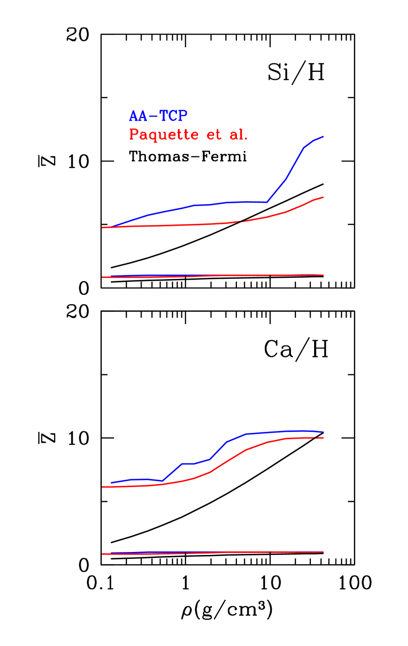
Figure 2: Average ion charges in a plasma of a trace ($x_{2}=0.001$) of silicon (upper panel) and calcium (lower panel) in hydrogen. The $(\rho,T)$ conditions correspond to the bottom of the superficial hydrogen convection zone of a 0.6 M_⊙ DA white dwarf cooling from $T_{\rm eff}=8500\,$K (left) to $5000\,$K. The abscissa is the density at the bottom of the convection zone, which increases as the WD cools (Table 2). The lower set of curves in each panel shows the charge of hydrogen, the upper set that of the heavier ion (Si or Ca). The charges computed from three models are shown: with the model used to calculate the Paquette et al. coefficients (Fontaine et al., 2015) (red), the AA-TCP plasma model Starrett & Saumon (2014a) (blue), and the simple Thomas-Fermi model (black, Stanton & Murillo (2016)). The first two models predict full ionization of H ($\bar{Z}=1$) but differ in their prediction of the charge of the heavier ion, most notably for Si. The lack of electronic shell structure in the Thomas-Fermi model results in a featureless increase of $\bar{Z}$. [See the electronic edition of the Journal for a color version of this figure.]

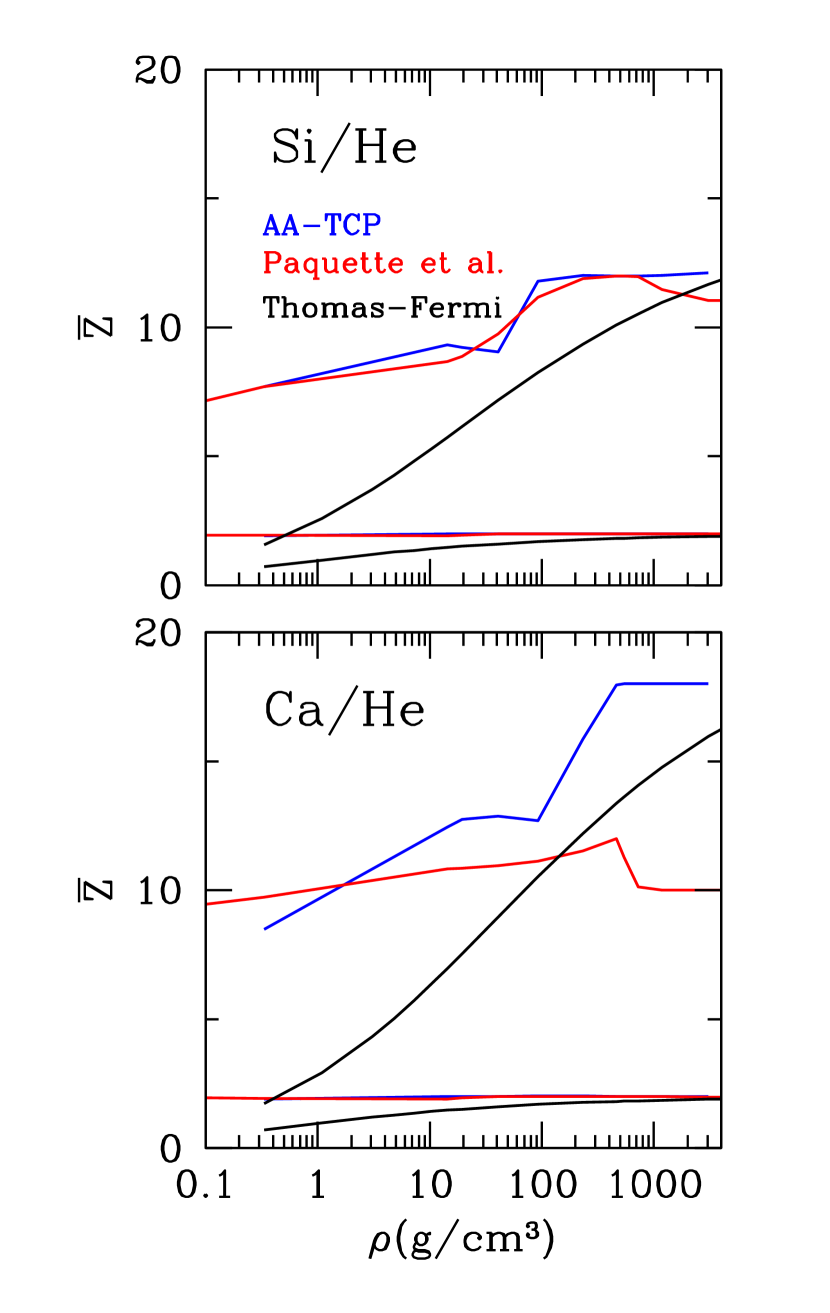
Figure 3: Same as Figure 2 but for traces of Si and Ca at the bottom of the superficial helium convection zone (Table 3). Both the Paquette et al. and the AA-TCP models predict that helium is fully ionized under these conditions ($\bar{Z}=2$). At the highest densities, Si retains only its $1s^{2}$ electrons ($\bar{Z}\sim 12$) in both models. For Ca, the AA-TCP model also predicts that only the $1s^{2}$ electrons remain bound. On the other hand, the model used by Paquette et al. predicts a much lower charge of ($\bar{Z}\sim 10$) for the Ca ion, retaining the full $n=2$ electronic shell. The lack of electronic shell structure in the Thomas-Fermi model results in a featureless increase of $\bar{Z}$. [See the electronic edition of the Journal for a color version of this figure.]

The charges of the Ca and Si ions at the bottom of the hydrogen convection zone are shown in Fig. 2. In this and subsequent figures, the density is used as the independent variable following the bottom of the convection zone for a cooling sequence of white dwarfs. The temperature also varies along the ordinate (see Tables 2 and 3). Under these conditions, hydrogen is always essentially fully ionized, the AA-TCP model predicting a slightly higher degree of ionization (by $\Delta{\bar{Z}}\lesssim 0.1$) at lower densities ($\sim 0.1$ - 1 g/cm³). The degree of ionization of Si in H is systematically larger in the AA-TCP model, especially at the higher density/temperatures where only the $1s^{2}$ electrons remain bound (${\bar{Z}}{\rm(Si)}\sim 12$) while the Fontaine et al. (2015) model predicts that it also retains most of the L-shell electrons (${\bar{Z}}$(Si)$\sim 7$). For Ca, the pattern of ionization is similar, with an increase toward higher densities and temperatures, but in this case both models predict nearly the same average charge for the Ca ions with the AA-TCP being systematically higher. In helium envelopes, the convection zone can reach to densities well above $10^{3}\,$g/cm³ where the plasma is strongly coupled and strongly degenerate. In all these cases, both models predict that He is fully ionized (Fig. 3). Interestingly, they predict very similar degrees of ionization for Si over this wide range of conditions while the Ca charges differ markedly above 100 g/cm³, with the AA-TCP model again predicting that Ca retains only its $1s^{2}$ electrons (${\bar{Z}}$(Ca)=18) and the simpler ionization model reaching a closed-shell Ne-like configuration (${\bar{Z}}$(Ca)=10). The simplest model to calculate ion charges while taking into account temperature and pressure ionization is the semi-classical Thomas-Fermi average atom model (Feynman et al. (1949), see Stanton & Murillo (2016) for a practical calculation of the ion charge). This model fares poorly at low density and temperatures where it predicts that H and He are only about 50% ionized. For heavier elements, the absence of electronic shell structure in the Thomas-Fermi model provides a very smooth transition towards full ionization but predicts ion charges that are quite different from the other two models over nearly the full range of conditions shown in Figures 2 and 3. Note that any reasonable ionization model must reach full ionization at high temperatures and high densities, hence the influence of the choice of ionization model on the diffusion coefficient must vanish at large enough depth in the star.

Figure 4 shows the coefficient of inter-diffusion of Si and Ca in hydrogen envelopes. The general trend of $D_{12}$ at the bottom of the convection zone of stars with decreasing $T_{\rm eff}$ is of a rapid decrease caused primarily by the increased density and coupling of the plasma. Larger densities and plasma coupling implies more frequent and stronger collisions, respectively, that both inhibit diffusion. Four calculations of $D_{12}$ are shown for both Si and Ca. For Si, the Paquette et al. result (solid red) and the EPT results (solid blue) agree remarkably well over the full range of conditions. This agreement is somewhat fortuitous, however. If the ion charges from the AA-TCP model that are used in the EPT calculation are also applied in the Paquette et al. model, $D_{12}$ decreases by $\sim 25$%. Thus for a given $Z$(Si), the static screened Coulomb potential of Paquette et al. leads to an underestimate of $D_{12}$ by about 25%. The classical molecular dynamics simulations (black squares), which are based on the same AA-TCP interaction potentials $V_{ij}(r)$ that leads to the potential of mean force $V_{ij}^{\rm eff}(r)$ used in the EPT calculation show a level of scatter that is greater than their formal statistical uncertainties (shown by error bars). This illustrates the difficulty in estimating accurate diffusion coefficients of trace species from molecular dynamics simulations. Nonetheless, the latter agree quite well with the EPT calculation within the scatter. The diffusion coefficient of Ca (lower panel of Fig. 4) shows the same general features. A comparison with $D_{12}$ evaluated with the fits of Stanton & Murillo (2016), using the same ion charges as the Paquette et al. calculation (solid red curve) shows remarkable agreement with differences that are almost always under 2% and no more than 3%, for both Ca and Si.

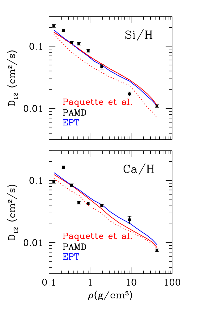
Figure 4: Coefficient of inter-diffusion of Si and Ca at the bottom of the superficial hydrogen convection zone (Table 2). Four calculations are shown: The value from Paquette et al. (red solid lines), from the PAMD classical molecular dynamics simulations (black squares), and from the effective potential theory (EPT, blue solid curves). The latter two calculations are based on the same ion-ion pair potential and ideally should give the same results. The Paquette et al. diffusion coefficient calculated with the ionic charges from the AA-TCP model are shown by the red dotted line. Under these conditions, the plasma is weakly coupled and the EPT agrees very well with Paquette et al. [See the electronic edition of the Journal for a color version of this figure.]

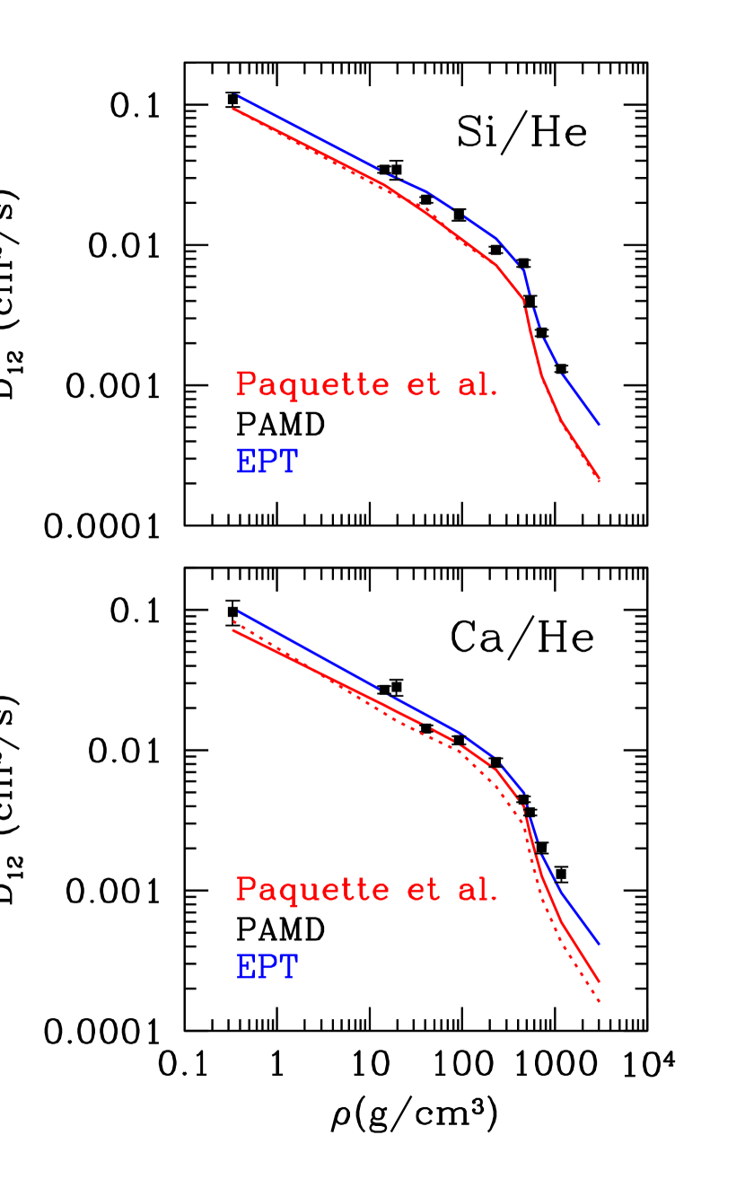
Figure 5: Same as Figure 4 but for the diffusion of Si and Ca at the bottom of the superficial hydrogen convection zone (Table 3). At the higher densities encountered in the cooler He WDs, the plasma is more strongly coupled and several assumptions in Paquette et al. (1986a) are no longer valid, resulting in an underestimation of the diffusion coefficient by up to a factor of 2.4. Note the different scale of the ordinate axis compared to Fig 4. [See the electronic edition of the Journal for a color version of this figure.]

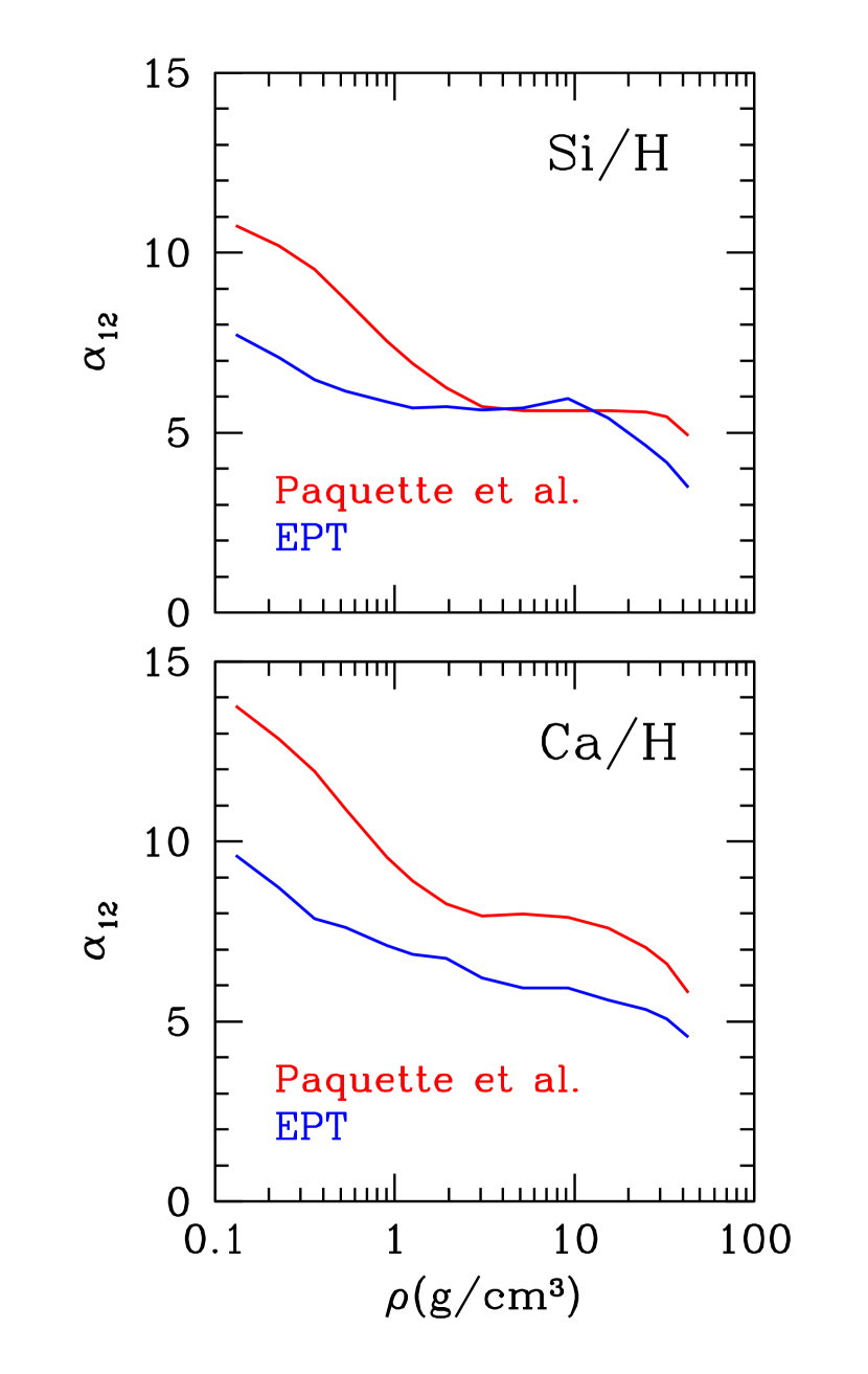
Figure 6: Coefficient of ionic thermal diffusion factor of Si and Ca at the bottom of the superficial hydrogen convection zone (Table 2) from the Paquette et al. and the EPT models. [See the electronic edition of the Journal for a color version of this figure.]

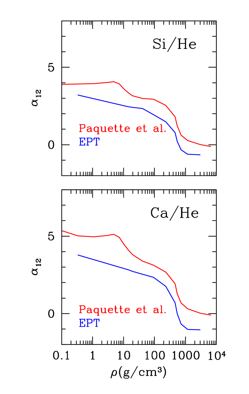
Figure 7: Same as Fig. 6 but showing the coefficient of ionic thermal diffusion factor of Si and Ca at the bottom of the superficial helium convection zone (Table 3). [See the electronic edition of the Journal for a color version of this figure.]

The coefficients of inter-diffusion of Si and Ca in helium envelopes behave in a similar fashion (Fig. 5) but differ from that in hydrogen envelopes. At densities above 400 g/cm³, $D_{12}$ drops rapidly due to the rapid increase of the Coulomb coupling between the heavy ions and the He²⁺ plasma as the convection zone in the He envelope reaches much deeper into the star. The scatter in the simulations is reduced compared to the hydrogen case because of the stronger coupling, which results in faster equilibration and convergence as well as smaller fluctuations. The EPT calculation is validated by the excellent agreement with the classical molecular dynamics simulations. As in the case of hydrogen, the Paquette et al. model systematically underestimates $D_{12}$ (more for Si than for Ca) by $\sim 35$% and up to a factor of 2.4 in He-envelope WDs with $T_{\rm eff}\sim 5600\,$K. This can be traced back to the more repulsive screened Coulomb potential compared to the potential of mean force (Figure 1). Interestingly, in this case the inter-diffusion coefficients of Stanton & Murillo (2016) agrees with Paquette et al. (solid red curves) to better than 1% at densities above 400 g/cm³ but they deviate from each other by $\sim 15$% at the lowest density of 0.3 g/cm³.

Figures 6 and 7 show the ionic contribution $\alpha_{12}$ to the thermal diffusion factor $\alpha_{\scriptscriptstyle T}$. Because it is defined as a pre-factor to $D_{12}$, most of the $\rho$–$T$ dependence of the ionic thermal diffusivity is taken up by $D_{12}$ and $\alpha_{12}$ depends only weakly on the plasma conditions and the charge of the heavy ion. It decreases steadily as the plasma coupling increases. For hydrogen envelopes, $\alpha_{12}$ is 2–3 times larger than in helium envelopes. We find that the Paquette et al. and EPT models are in generally good agreement although the former systematically overestimates $\alpha_{12}$ by 20–40%. In particular, the EPT model predicts that $\alpha_{12}$ changes sign in the strongest coupling regimes encountered in the He envelopes (Figure 7). This also happens in the Paquette et al. (1986a) calculation but to a much smaller extent. A negative $\alpha_{12}$ implies that thermal diffusion will tend to make the heavy species move upward in the star. However, the ionic thermal diffusion term is typically 10–30 times smaller than the gravitational settling terms in Equation 1 under the conditions of interest.

These calculations show that for the same ionic charges, the AA-TCP plasma model combined with the EPT gives diffusion coefficients $D_{12}$ that are systematically higher than those of Paquette et al. (1986a). The difference is modest $\lesssim 35$% when the plasma coupling is moderate as in all H envelopes but grows to a factor of $\gtrsim 2$ in cool He envelopes ($T_{\rm eff}\lesssim 15000\,$K) where the plasma is strongly coupled. The dimensionless ionic thermal diffusion factor $\alpha_{12}$ is generally lower in the EPT calculation by an amount that is essentially independent of the plasma coupling. The dependence of $D_{12}$ on the charge of the heavy ion (the light ions H or He being fully ionized at the bottom of the convection zone) is significant. The ionization model of Fontaine et al. (2015) used here to compute the nominal Paquette et al. (1986a) diffusion coefficients gives charges that can be in very good agreement with those of the AA-TCP plasma model but are typically lower, and sometimes considerably so. This tends to compensate for the intrinsic difference in the theory used to evaluate $D_{12}$. This is a cautionary statement about the importance of the ionization model and the underlying equation of state model in evaluating transport coefficients in white dwarf envelopes.

4 Diffusion time scales at the bottom of the convection zone

One of the most remarkable recent developments in the field of white dwarfs is the recognition that the presence of metal lines in the spectra of DZ, DBZ and DAZ white dwarfs originates from the accretion of planetary material (Jura, 2003; Jura & Young, 2014; Farihi, 2016). This provides a unique window into the detailed elemental composition of the accreted planetary solids that is not otherwise accessible from the observation of exoplanets. The observed photospheric abundance pattern of metals results from the interplay of the composition of the accreted material, the accretion rate, and the processes of convective mixing and diffusion. Thus, the composition of the infalling material that is deduced is sensitive to the relative diffusion time scale of the various accreted elements. As an illustration, we consider the evolution of the surface mass fraction $X_{2}$ of a trace heavy element in the convection zone of a white dwarf that is accreting at a constant rate $\dot{M_{2}}$ (Dupuis et al., 1993)

$$\frac{dM_{2}}{dt}=\frac{d(X_{2}M_{\scriptscriptstyle\rm CZ})}{dt}=\dot{M_{2}}+4\pi R_{\scriptscriptstyle\rm CZ}^{2}\rho X_{2}w_{12}.$$ (15)

If we assume that $M_{\scriptscriptstyle\rm CZ}$, $R_{\scriptscriptstyle\rm CZ}$ and $w_{12}$ are constant, the solution is

$$X_{2}(t)=X_{2}(0)e^{-t/\tau_{\rm d}}+\frac{\tau_{\rm d}\dot{M_{2}}}{M_{\scriptscriptstyle\rm CZ}}(1-e^{-t/\tau_{\rm d}})$$ (16)

where $\tau_{\rm d}$ is the diffusion time scale of species 2 at the bottom of the convection zone, given by

$$\tau_{\rm d}=\frac{-M_{\scriptscriptstyle\rm CZ}}{4\pi R_{\scriptscriptstyle\rm CZ}^{2}}\frac{1}{\rho w_{12}}.$$ (17)

This diffusion time scale can be evaluated from the quantities given in Tables 2 and 3 and $w_{12}$ using Equation 1. Note that for downward diffusion, $w_{12}<0$ and $\tau_{\rm d}>0$. At late times ($t\gg\tau_{\rm d}$) the abundance of the trace metal reaches an equilibrium value of

$$X_{2}^{\rm eq}=\frac{\tau_{\rm d}\dot{M_{2}}}{M_{\scriptscriptstyle\rm CZ}}.$$ (18)

After accretion has stopped ($\dot{M_{2}}=0$) the mass fraction decreases exponentially

$$X_{2}(t)=X_{0}e^{-t/\tau_{\rm d}}.$$ (19)

Dupuis et al. (1993) and Bauer & Bildsten (2018) have studied the evolution of such a trace metal abundance in a white dwarf undergoing episodic accretion.

We are interested in how our improved model of diffusion in dense plasmas affects the relative diffusion time scale of Ca and Si and the inferred composition of the accreted planetary material. In the accretion/diffusion equilibrium limit, the observed ratio of mass fractions of the accreted material is related to the ratio of diffusion time scales

$$\frac{X_{\scriptscriptstyle\rm Si}}{X_{\scriptscriptstyle\rm Ca}}=\frac{\tau_{\rm d}({\rm Si})}{\tau_{\rm d}({\rm Ca})}\frac{\dot{M}_{\rm Si}}{\dot{M}_{\rm Ca}},$$ (20)

and in the case of no accretion, this ratio evolves exponentially on a time scale of the order of the shorter of the two diffusion time scales

$$\frac{X_{\scriptscriptstyle\rm Si}}{X_{\scriptscriptstyle\rm Ca}}=\frac{X_{0}({\rm Si})}{X_{0}({\rm Ca})}\exp\bigg{[}-t\Big{(}\frac{1}{\tau_{\rm d}({\rm Si})}-\frac{1}{\tau_{\rm d}({\rm Ca})}\Big{)}\bigg{]}.$$ (21)

For the present purpose, we approximate the diffusion velocity by neglecting the ordinary and thermal diffusion terms

$$w_{12}=D_{12}\Big{[}\Big{(}\frac{Z_{2}}{Z_{1}}A_{1}-A_{2}\Big{)}\frac{m_{0}g_{\scriptscriptstyle\rm CZ}}{k_{\scriptscriptstyle\rm B}T}+\Big{(}\frac{Z_{2}}{Z_{1}}-1\Big{)}\frac{\partial\ln P_{i}}{\partial r}\Big{]}.$$ (22)

For a given stellar structure, the ratio $\tau_{\rm d}$(Si)/$\tau_{\rm d}$(Ca) depends only on the values of $D_{12}$ and $Z_{2}$ for each element. The charge $Z_{2}$ also enters indirectly through $D_{12}$ (Figures 4 and 5). As we have seen above, a larger ion charge for the trace element $Z_{2}$ results in a smaller $D_{12}$, a smaller pre-factor in Equation 22, and a longer diffusion time scale.

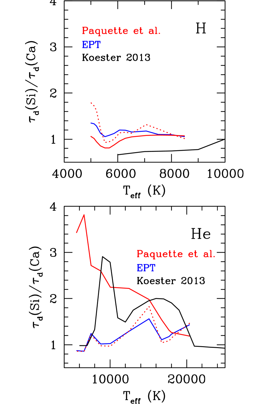
Figure 8: Ratio of the diffusion time scales of Si and Ca at the bottom of the convection zone for H (top panel) and He (bottom panel) envelopes. The Paquette et al. (1986a) calculation is shown for ion charges from the Fontaine et al. (2015) ionization model and the AA-TCP model with solid and dotted red lines, respectively (see Figures 2 and 3). The ratios based on the AA-TCP model and the EPT theory are shown in blue. The calculation of Koester (2013) is shown in black. Unlike in the preceding figures, the abscissa is the effective temperature of a 0.6 M_⊙ white dwarf that evolves to the left as it cools (Tables 2 and 3). The two panels are plotted on different $T_{\rm eff}$ scales. See text for details. [See the electronic edition of the Journal for a color version of this figure.]

Figure 8 shows the ratio of diffusion time scales of Ca and Si in H and He white dwarf envelopes as a function of $T_{\rm eff}$ along the cooling sequences of Tables 2 and 3. For each case, we present the 1) Paquette et al. calculation, 2) the Paquette et al. calculation but with the ion charges from the AA-TCP plasma model, 3) the EPT calculation and 4) the results of Koester (2013). For diffusion in H envelopes, we find that Ca and Si diffuse at approximately the same time scale for the range studied here ($T_{\rm eff}=5000$ – 8500 K). Substituting the charges from the AA-TCP model in the Paquette et al. formalism increases the diffusion time scale of Si because of the larger ${\bar{Z}}$(Si) (Figure 2). The effect becomes significant for the coolest H-rich stars, almost reaching a factor of two. Switching to the EPT calculation somewhat compensates for the higher charge of Si ions and the difference with Paquette et al. is $\lesssim 20$%. The behavior in He envelopes is quite different. Here the ratio of diffusion time scales from Paquette et al. ranges from $\sim 1.1$ at $T_{\rm eff}\sim 20000\,$K to greater than 3 for $T_{\rm eff}$ below 7500 K. Applying the AA-TCP charges to the Paquette et al. calculation brings it in excellent agreement with the EPT calculation, which is generally well below the former result. The much larger charge of Si obtained with the AA-TCP model in the deep convection zones of low-$T_{\rm eff}$ envelopes accounts for the large drop in the time scale ratio. Thus, in DZ (He-rich) stars with $T_{\rm eff}<10000\,$K, the EPT theory (and the underlying AA-TCP plasma model) predicts a diffusion time scale ratio $\tau_{\rm d}$(Si)/$\tau_{\rm d}$(Ca) at the bottom of the convection zone that is about one third of that predicted with the Paquette et al. model.

We further compare the ratio of diffusion time scales with the results of Koester (2009) as updated in Koester (2013). Both use the Paquette et al. (1986a) fits to the collision integrals. Those are shown by the black lines in Figure 8. A detailed discussion is not possible because the physical conditions at the bottom of the convection zone where the diffusion time scales are evaluated are not given in Koester (2013), but the pressures, temperatures and masses of the convection zone of Koester (2009) are close to those in Tables 2 and 3. The ion charges are calculated with an independent ionization model and are not specified, however. For diffusion in hydrogen envelopes, $\tau_{\rm d}$(Si)/$\tau_{\rm d}$(Ca) is systematically lower than Paquette et al. and the EPT calculations by 40% to 80%. This probably arises from a combination of different stellar structures and ionization model. More striking is the case of helium envelopes where large deviations between Paquette et al. and EPT are found, with considerable variation with $T_{\rm eff}$. The double hump structure seen in the Koester (2013) curve is very likely due to the ionization model as the peaks occur approximately where changes in ionization due to electronic shells are expected. This again highlights the importance of the ionization model in computing diffusion time scales.

In the cases of equilibrium and episodic accretion, a factor of $\sim 3$ change in the ratio of diffusion time scales leads to significant changes in the inferred composition of the accreted material. The latter often departs from that measured in meteorites and solar system bodies and varies from star to star, leading to various interpretations regarding other planetary systems and their evolution at very late stages of stellar evolution (see, for example, Raddi et al. (2015), Kawka & Vennes (2016), Hollands et al. (2018), Harrison et al. (2018), Doyle et al. (2019)). It would be prudent to consider that the inferred composition of the accreted material is affected by uncertainties in the diffusion coefficients that are not negligible, particularly in cool He-rich white dwarfs.

4.1 Other mixing processes

The description of convection with the mixing length theory used here is rather simplistic. Two processes, thermohaline mixing and convective overshooting at the bottom of the convection zone, can increase the effective extent of mixing (i.e. $M_{\scriptscriptstyle\rm CZ}$) considerably. The metal enrichment of the upper layers of a white dwarf that is accreting solid material causes an inverted molecular weight gradient that can trigger a thermohaline (double diffusive) instability (Deal et al., 2013; Wachlin et al., 2017; Bauer & Bildsten, 2018, 2019). Because it is driven by the gradient of molecular weight, the thermohaline instability is favored by higher accretion rates on white dwarfs with thin superficial convection zones where the accreted material is more concentrated. Bauer & Bildsten (2019) have shown that thermohaline mixing has a minimal effect in DA white dwarfs with $T_{\rm eff}\lesssim 9000\,$K and in DB white dwarfs below 18000 K. Our study of diffusion coefficients focuses on white dwarfs near these limits and cooler (Tables 2 and 3), thus thermohaline mixing will not affect our results.

Convective overshooting is caused by the momentum of downward moving fluid plumes that allows them to move past the convective/radiative boundary as defined by the Schwarzschild criterion in 1-dimensional stellar models. These fluid parcels are decelerated as they move in the convectively stable region but provide effective mixing well below the boundary calculated from the mixing length theory. Three-dimensional radiative hydrodynamics simulations of convection in white dwarfs indicate that the mixing due to overshooting extends over a few pressure scale heights and increases the mass of the mixed region $M_{\scriptscriptstyle\rm CZ}$ by up to 2.5 orders of magnitude (Tremblay et al., 2015; Kupka et al., 2018; Cunningham et al., 2019). Those studies have so far been limited to hydrogen envelopes and $T_{\rm eff}>11400\,$K (for $\log g=8$), which is above the range of our study of diffusion coefficients. Little is known about overshooting in the cooler hydrogen or helium envelopes relevant to this study. Nonetheless, we can make a general observation as to how overshooting bears on our results.

The net effect of convective overshooting is to increase the depth where metals diffuse out of the convection zone, increasing $M_{\scriptscriptstyle\rm CZ}$. Everything else being equal, it implies a higher accretion rate for a given observed surface abundance, as suggested by Equation (18). At deeper levels, the temperature, density, as well as the plasma coupling and degeneracy will be higher than the values reported in Tables 2 and 3. However, our white dwarf evolution sequences show that a two order of magnitude increase in $M_{\scriptscriptstyle\rm CZ}$ results in an increase in temperature of $\Delta\log T\lesssim 0.5$ and of $\Delta\log\rho\lesssim 1.5$ at the bottom of the mixing region. The plasma coupling parameter of the background element (H or He) increases by a modest factor of 1 – 1.4. At higher densities and temperatures the charge of the heavy ion will be larger, increasing the ion-background coupling that primarily affects the diffusion coefficient. Taking overshooting into account, we expect the differences in the ratio $\tau_{\rm d}({\rm Si})/\tau_{\rm d}({\rm Ca})$ between models to be very similar if not larger than those shown in Figure 8.

5 Conclusion

We have revisited the calculation of diffusion coefficients using an advanced model for the partially ionized plasma found in the envelopes of cool white dwarfs. This model combines an average atom model with the integral equations of fluid theory for a two-component plasma of classical ions and quantum electrons (the “AA-TCP” model). This plasma model describes self-consistently the bound and free electronic states and the interactions between ions and electrons for any degree of plasma coupling and electron degeneracy. It accounts for temperature and pressure ionization equally well without introducing somewhat heuristic concepts such as continuum lowering or occupation probabilities. The model solves for the average charge of the ions, the interaction potentials and the correlation functions. The ionic pair distribution function can then be used in an extension of the Boltzmann equation called Effective Potential Theory (“EPT”) to compute ionic transport coefficients, such as the inter-diffusion coefficient and the thermal diffusion factor. We have looked at the diffusion coefficients of Ca and Si ions at the bottom of the convection zone of cool white dwarfs with hydrogen and helium envelopes, and compared with the widely used coefficients of Paquette et al. (1986a).

For the same set of conditions, we have calculated the coefficient of diffusion $D_{12}$ with the Paquette et al. (1986a) formalism as modified by Fontaine et al. (2015), with the Effective Potential Theory and with classical molecular dynamics. The latter two methods are based on the same ion-ion pair potential obtained from the AA-TCP model and we find excellent agreement within the uncertainty and scatter of the molecular dynamics simulations, which further validates the EPT in this application.

We have shown that in weakly to moderately coupled plasmas, the Paquette et al. (1986a) calculation of $D_{12}$ is very good but becomes increasingly inaccurate as the plasma becomes more strongly coupled. In the context of stellar astrophysics, the Paquette et al. (1986a) approach is perfectly adequate for all normal stars where the plasma is weakly coupled, as well as for all DA white dwarfs and DB white dwarfs with $T_{\rm eff}\gtrsim 15000\,$K. In cooler white dwarfs with helium envelopes, some of the assumptions underlying the Paquette et al. (1986a) coefficients become inadequate, resulting in diffusion coefficients that are underestimated by over a factor of two in the coolest models. The ionic thermal diffusion factor $\alpha_{12}$ is generally in good agreement between the two calculations with the EPT value being $\sim 20$% lower across all coupling regimes.

The diffusion coefficients of Paquette et al. (1986a), Fontaine et al. (2015), Koester (2009) and Stanton & Murillo (2016) all based on the evaluation of the collision integrals that appear in the Chapman-Enskog solution or the resistance coefficients of Burgers, with a static screened Coulomb (i.e. Yukawa) potential for the ion-ion interaction. However, they differ in how the ion charge is calculated and thus in their ion-ion potentials, even though they share the same Yukawa functional form. The calculation of the ionization of a metal in white dwarf envelopes involves pressure ionization and is challenging, and the resulting uncertainty in the diffusion coefficients was acknowledged early on (Dupuis et al., 1992). We investigated this effect by computing $D_{12}$ with the Paquette et al. (1986a) model with the Fontaine et al. (2015) model of ionization and with the charges obtained with the AA-TCP model that has the most realistic microscopic plasma physics of the models considered here. We found that the average ionic charge of the heavy ion can vary substantially between models and that $D_{12}$ is affected at the $\sim 30$% level. A further consideration, which we did not address, is that the heavy element will have a distribution of charge states, each with a different $D_{12}$. In this case, a proper description of diffusion would be to treat each ionization stage as a separate species rather than the diffusion of an ion with an average charge (Dupuis et al., 1992; Koester, 2009; Bauer & Bildsten, 2019).

For simplicity and for illustration purposes, we considered diffusion time scales at the base of the convection zone as defined by the mixing length theory and the Schwarzschild stability criterion in 1-dimensional models. The thermohaline instability and convective overshooting are two processes that can extend vertical mixing to much greater depths. The thermohaline instability occurs only in white dwarfs that are hotter than those we considered here (Bauer & Bildsten, 2018, 2019), i.e. in stars where the plasma is weakly coupled and the Paquette et al. (1986a) coefficients are reliable. Three-dimensional simulations of convective overshooting in white dwarfs show that the mixing zone can extend much deeper than the nominal convection zone obtained with the mixing length theory. However, the corresponding increase in plasma coupling at the bottom of the mixing layer, and therefore the decrease in $D_{12}$, is modest, with little consequence on our results.

Our results are of immediate relevance to the determination of the composition of accreted solid planetesimals from the observed abundance of metals in the atmospheres of white dwarfs. The elemental planetesimal composition inferred from the accretion/diffusion scenario provides important information as to the nature and origin of mature exoplanetary systems (Xu et al., 2013; Hollands et al., 2018). The abundance of oxygen in particular has recently been shown to provide a measure of its fugacity in the solid accreted material which is an important clue to its geochemistry (Doyle et al., 2019). This composition depends strongly on the relative diffusion time scales of the various elements. We found that the ratio of diffusion time scales between Si and Ca changes by over a factor of three in cool DZ stars when applying a more sophisticated theory for the dense plasma and the calculation of diffusion coefficients than the widely used Paquette et al. (1986a) diffusion coefficients. In this study, we focused on two elements that are common in polluted white dwarfs, Si and Ca, which are somewhat similar with atomic numbers of 14 and 20, respectively. DZ stars show a much broader range of elements in their spectra, from C to Sr (Xu et al., 2013), and we expect that updated diffusion coefficients will deviate from Paquette et al. accordingly. It would be of interest to extend this work to other heavy elements commonly observed in cool DZ stars, as well as to the diffusion of non-trace mixtures, such as the inter-diffusion of H and He and of C and He.

To summarize, the model applied here combines a sophisticated plasma model and a modification of the Chapman-Enskog theory of transport in plasmas that provides a valuable compromise between physical realism and computational cost. The Paquette et al. (1986a) formalism is perfectly suitable in weakly coupled plasmas and has the considerable advantage that the collision integrals can be calculated once and for all and scaled to any mixture of ions a posteriori. Our approach requires a separate tabulation for each element pair or mixture. The accuracy gained in the diffusion coefficients in cool white dwarfs and the astrophysical implications of the new coefficients should motivate such an effort. This initial application of the AA-TCP plasma model with the EPT theory to diffusion in white dwarfs demonstrates that advances in the modeling of dense plasmas can have important astrophysical consequences.

References

- Aller & Chapman (1960) Aller, L. H. & Chapman, S. 1960, ApJ, 132, 461
- Althaus & Benvenuto (2000) Althaus, L. G. & Benvenuto, O.J. 2000, MNRAS, 317, 952
- Bastea (2005) Bastea, S. 2005, Phys. Rev. E, 71, 056405
- Baalrud & Daligault (2013) Baalrud, S.D. & Daligault, J. 2013, Phys. Rev. Lett., 110, 235001
- Baalrud & Daligault (2015) Baalrud, S.D. & Daligault, J. 2015, Phys. Rev. E, 91, 063107
- Baalrud & Daligault (2019) Baalrud, S.D. & Daligault, J. 2019, Phys. Plasmas, 26, 082106
- Bauer & Bildsten (2018) Bauer, E.B. & Bildsten, L. 2018, ApJ, 859, 19
- Bauer & Bildsten (2019) Bauer, E.B. & Bildsten, L. 2019, ApJ, 872, 96
- Beznogov & Yakovlev (2014) Beznogov, M.V. & Yakovlev, D.G. 2014, Phys. Rev. E90, 033102
- Blouin et al. (2019) Blouin, S., Dufour, P., Thibeault, C., & Allard, N. 2019, ApJ, 878, 63
- Brassard & Fontaine (2014) Brassard, P. & Fontaine, G. 2014, ASP Conf. Ser., 481, 221
- Burakovzky et al. (2013) Burakovsky, L., Ticknor, C., Kress, J.D., Collins, L.A. & Lambert, F. 2013, Phys. Rev. E87, 023104
- Burgers (1969) Burgers, J.M. 1969, Flow Equations for Composite Gases, (New York: Academic)
- Chapman & Cowling (1970) Chapman, S. & Cowling, T.G. 1970 The mathematical theory of uniform gases (Cambridge: Cambridge University Press)
- Chayer et al. (1995) Chayer, P., Fontaine, G. & Wesemael, F. 1995, ApJS, 99, 189
- Cunningham et al. (2019) Cunningham, T., Tremblay, P.-E., Freytag, B., Ludwig, H.-G. & Koester, D. 2019, MNRAS, 488, 2503
- Daligault (2012) Daligault, J. 2012, Phys. Rev. Lett.108, 225004
- Daligault et al. (2016) Daligault, J., Baalrud, S.D., Starrett, C.E., Saumon, D. & Sjostrom, T. 2016, Phys. Rev. Lett.116, 075002
- Danel, Kazandjian & Zérah (2012) Danel, J.-F., Kazandjian, L. & Zérah, G. 2012, Phys. Rev. E85, 066701
- Deal et al. (2013) Deal, M., Deheuvels, S., Vauclair, G., Vauclair, S. & Wachlin, F.C. 2013, A&A, 557, L12
- Doyle et al. (2019) Doyle, A.E., Young, E.D., Klein, B., Zuckerman, B. & , Schlichting, H. 2019, , Science, 366, 356
- Dufour et al. (2007) Dufour, P., Bergeron, P., Liebert, J., Harris, H.C., Knapp, G.R., Anderson, S.F., Hall, P.B., Strauss, M.A., Collinge, M.J. & Edwards, M.C. 2007, ApJ, 663, 1291
- Dupuis et al. (1992) Dupuis, J., Fontaine, G., Pelletier, C. & Wesemael, F. 1992, ApJS, 82, 505
- Dupuis et al. (1993) Dupuis, J., Fontaine, G., Pelletier, C. & Wesemael, F. 1993, ApJS, 84, 73
- Eliezer et al. (2002) Elizier, S., Ghatak, A. & Hora, H. 2002 Fundamentals of equations of state (World Scientific, New Jersey), Chap. 8
- Farihi (2016) Farihi, J. 2016, New Astron. Rev., 71, 1
- Feynman et al. (1949) Feynman, R.P., Metropolis, N. & Teller, E., 1949, PhRv, 75, 1561
- Fontaine & Michaud (1979) Fontaine, G. & Michaud, G., 1979, ApJ231, 826
- Fontaine, Brassard & Bergeron (2001) Fontaine, G., Brassard, P. & Bergeron, P., 2001, PASP113, 409
- Fontaine et al. (2015) Fontaine, G., Brassard, P., Dufour, P. & Tremblay, P.-E., 2015, ASP Conf. Ser. 493, 113
- French et al. (2012) French, M. Becker, A., Lorenzen, W., Nettelmann, N. Bethkenhagen, M., Wicht, J. & Redmer, R. 2012, ApJS, 202, 5
- García-Berro et al. (2010) García-Berro, E., Torres, S., Althaus, L.G., Renedo, I., Lorén-Aguilar, P., Córsico, A.H., Rohrmann, R.D., Salaris, M. & Isern, J. 2010, Nature465, 194
- Grabowski et al. (2020) Grabowski, P. E., Hansen, S.B., Murillo, M.S. and 37 authors 2020, submitted to High Ener. Dens. Phys.
- Green (1954) Green, M. S. 2020, J. Chem. Phys. 22, 398
- Hansen & McDonald (2013) Hansen, J.-P. & McDonald, I. R. 2013, Theory of simple liquids, Chap. 7 (Oxford: Academic Press)
- Hansen, McDonald & Pollock (1975) Hansen, J.-P., McDonald, I. R. & Pollock, E.L. 1975, Phys. Rev. A11, 1025
- Hansen, McDonald & Vieillefosse (1975) Hansen, J.-P., McDonald, I. R. & Vieillefosse, P. 1979, Phys. Rev. A20, 2590
- Harrison et al. (2018) Harrison, J.H.D., Bonsor, A. & Madhusudhan, N. 2018, MNRAS479, 3814
- Haxhimali et al. (2014) Haxhimali, T., Rudd, R., Cabot, W.H. & Graziani, F. 2014, Phys. Rev. E, 90, 023104
- Hollands et al. (2018) Hollands, M.A., Gänsicke, B.T. & Koester, D. 2018, MNRAS477, 93
- Hummer & Mihalas (1988) Hummer, D. G. & Mihalas, D. 1988, ApJ331, 794
- Iben & McDonald (1985) Iben, I. Jr. & MacDonald, J. 1985, ApJ296, 540
- Jakse & Pasturel (2013) Jakse, N. & Pasturel, A. 2013, Scientific Rep. 3, 3135
- Jura (2003) Jura, M. 2003, ApJ594, 91
- Jura & Young (2014) Jura, M. & Young, E.D. 2014, Ann. Rev. Earth Plan. Sci. 42, 45
- Kawka & Vennes (2016) Kawka, A. & Vennes, S., 2016, MNRAS, 458, 325
- Koester (2009) Koester, D. 2009, A&A, 498, 517
-
Koester (2013)
Koester, D. 2013, http://www1.astrophysik.uni-kiel.de/ koester/
astrophysics/astrophysics.html - Koester et al. (2014) Koester, D., Gänsicke, B. T. and Fahiri, J. 2014, A&A, 566, 34
- Kress et al. (2011) Kress, J.D., Cohen, J.S., Kilcrease, D.P., Horner, D.A. & Collins, L.A. 2011, Phys. Rev. E, 83, 026404
- Kupka et al. (2018) Kupka, F., Zaussinger, F. & Montgomery, M.H. 2018, MNRAS, 474, 4660
- Kubo (1957) Kubo, R. 1957, J. Phys. Soc. Japan, 12, 570
- Lambert, Clérouin & Mazevet (2006) Lambert, F., Clérouin, J. & Mazevet, S. 2006, Europhys. Lett. 75, 681
- Liboff (1959) Liboff, R.L. 1959, Phys. Fluids, 2, 40
- Macquarrie (1976) McQuarrie, D. A. 1976, Statistical Mechanics, (Harper & Row: New York)
- Mason et al. (1967) Mason, E.A., Munn, R.J. & Smith, F.J. 1967, Phys. Fluids, 10, 1827
- Meyer et al. (2015) Meyer, E.R., Kress, J.D., Collins, L.A. & Ticknor, C. 2014, Phys. Rev. E, 90, 043101
- Michaud (1970) Michaud, G. 1970, ApJ, 160, 641
- Michaud et al. (1976) Michaud, G., Charland, Y., Vauclair, S. & Vauclair, G. 1976, ApJ, 210, 447
- Muchmore (1984) Muchmore, D.O. 1984, ApJ, 278, 769
- Paquette et al. (1986a) Paquette, C., Pelletier, C., Fontaine, G. & Michaud, G., 1986a, ApJS, 61, 177
- Paquette et al. (1986b) Paquette, C., Pelletier, C., Fontaine, G. & Michaud, G., 1986b, ApJS, 61, 197
- Paxton et al. (2015) Paxton, B., Marchant, P., Schwab, J., Bauer, E.B., Bildsten, L., Cantiello, M., Dessart, L., Farmer, R., Hu, H., Langer, N., Townsend, R.H.D., Townsley, D.M. & Timmes, F.X. 2015, ApJS, 220, 15
- Pelletier et al. (1986) Pelletier, C., Fontaine, G., Wesemael, F., Michaud, G. & Wegner, G. 1986, ApJ, 307, 242
- Raddi et al. (2015) Raddi, R., Gänsicke, B.T., Koester, D., Farihi, J., Hermes, J.J., Scaringi, S., Breedt, E. & Girven, J. 2015, MNRAS, 450, 2083
- Rudd et al. (2012) Rudd, R.E., Cabot, W.H., Caspersen, K.J., Greenough, J.A., Richards, D.F., Streitz, F.H. & Miller, P.L. 2012, Phys. Rev. E, 85, 031202
- Salin & Gilles (2006) Salin G., & Gilles, D. 2006, J. Phys. A: Math. Gen., 39, 4517
- Saumon & Starrett (2020) Saumon, D., & Starrett, C.E. 2020, in Shock Compression of Condensed Matter – 2019, AIP Conference proceedings, ed. T. Germann, M. Lane, M. Armstrong, in press.
- Saumon et al. (2014) Saumon, D., Starrett, C.E., Anta, J.A., Daughton, W. & Chabrier, G. 2014, in Frontiers and Challenges in Warm Dense Matter, Lecture Notes in Computational Science and Engineering 96, ed. F. Graziani, M.P. Desjarlais, R. Redmer, S.B. Trickey, (Springer: Switzerland) p151
- Schatzman (1958) Schatzman, E. 1958, White Dwarfs, (Amsterdam: North-Holland)
- Shaffer et al. (2017) Shaffer, N.R., Baalrud, S.D. & Daligault J. 2017, Phys. Rev. E, 95, 013206
- Sjostrom & Daligault (2015) Sjostrom, T. & Daligault, J. 2015, Phys. Rev. E, 92, 063304
- Stanton & Murillo (2016) Stanton, L.G. & Murillo, M.S. 2016, Phys. Rev. E, 93, 043203
- Starrett & Saumon (2013a) Starrett, C.E. & Saumon, D. 2013a, Phys. Rev. E, 87, 013104
- Starrett & Saumon (2013b) Starrett, C.E. & Saumon, D. 2013b, Phys. Rev. E, 88, 059901(E)
- Starrett & Saumon (2014a) Starrett, C.E. & Saumon, D. 2014a, High. Ener. Dens. Phys., 10, 35
- Starrett & Saumon (2014b) Starrett, C.E., Saumon, D., Daligault, J. & Hamel, S. 2014b, Phys. Rev. E, 90, 033110
- Starrett et al. (2015a) Starrett, C.E., Daligault, J. & Saumon , D. 2015a, Phys. Rev. E, 91, 033101
- Starrett & Saumon (2015b) Starrett, C.E. & Saumon , D. 2015b, Phys. Rev. E, 92, 033101
- Starrett & Saumon (2016) Starrett, C.E. & Saumon, D. 2016, Phys. Rev. E, 93, 063206
- Ticknor et al. (2015) Ticknor, C., Collins, L.A. & Kress, J.D. 2015, Phys. Rev. E, 92, 023101
- Ticknor et al. (2016) Ticknor, C., Kress, J.D., Collins, L.A., Clérouin, J., Arnault, P. & Decoster, A. 2016, Phys. Rev. E, 93, 063208
- Tremblay et al. (2015) Tremblay, P.-E., Ludwig, H.-G., Freytag, B., Fontaine, G., Steffen, M. & Brassrad, P. 2015, ApJ, 799, 142
- Wachlin et al. (2017) Wachlin, F.C., Vauclair, G., Vauclair, S., & Althaus, L.G. 2017, A&A, 601, A13
- Xu et al. (2013) Xu, S., Jura, M., Klein, B., Koester, D. & Zuckerman, B. 2013, ApJ, 766, 132
- Zeidler-K. T. et al. (1986) Zeidler-K. T., E.M., Weidemann, V. & Koester, D. 1986, A&A, 155, 356