Safe Learning-based Observers for Unknown Nonlinear Systems using Bayesian Optimization

Abstract

Data generated from dynamical systems with unknown dynamics enable the learning of state observers that are: robust to modeling error, computationally tractable to design, and capable of operating with guaranteed performance. In this paper, a modular design methodology is formulated, that consists of three design phases: (i) an initial robust observer design that enables one to learn the dynamics without allowing the state estimation error to diverge (hence, safe); (ii) a learning phase wherein the unmodeled components are estimated using Bayesian optimization and Gaussian processes; and, (iii) a re-design phase that leverages the learned dynamics to improve convergence rate of the state estimation error. The potential of our proposed learning-based observer is demonstrated on a benchmark nonlinear system. Additionally, certificates of guaranteed estimation performance are provided.

1 Introduction

With modern dynamical systems growing in complexity, data-driven methods of state estimation have gained relevance and provide a suitable solution for problems with incomplete model knowledge, such as systems with unknown or unmodeled dynamics. Leveraging data generated from these systems and employing function approximators (such as neural networks) allows one to design controllers and estimators despite incomplete model descriptions, by identifying the unknown dynamics. While the most common applications of learning via function approximators are in identifying dynamical systems from measurement data [1, 2], approximating control laws using offline data [3, 4], or adapting with data to generate optimal control policies online [5, 6], the utility of data and approximators for state estimation in nonlinear systems with unmodeled dynamics remains relatively unexplored.

Some early investigations into data-driven observers, for example, in [7] assume model availability. However, the current wave of data-driven control has demonstrated the effectiveness of approximators in controlling systems with partial models or, in some cases, a ‘model-free’ manner. Data-driven observers in the model-free setting were explored almost two decades ago in [8], where the authors proposed an adaptation rule for learning the weights of a linear-in-parameter neural network (LPNN) that results in uniformly ultimately bounded estimation error dynamics. Although this work has been adopted in multiple applications such as robot control [9, 10], rotors [11], and more recently, wind turbines [12], the inherent assumptions and theory have hardly evolved. In most of these methodologies, the activation functions are considered to be radial basis functions, there is no measurement noise, and the theoretical guarantees of learning performance remain the same; an exception is [12] where the authors investigate input-to-state stability (ISS) observers for the known component of the model, but the learner performance is not ISS, and the learner’s weights require manual tuning.

In [13], the authors studied the problem of learning-based observer design for a class of partial differential equations (PDEs). The idea is based on designing a robust controller with respect to the structured model uncertainties, complemented with a learning layer, to auto-tune the observer gains, using a data-driven extremum seeking algorithm. However, the model uncertainties were compensated for by a robust estimation approach, and no online estimation of the model was proposed in this work. In [14], the authors proposed a learning-based observer design for the particular case of the Boussinesq PDE equations with parametric uncertainties, for a thermo-fluid application. The main idea is to construct a nominal observer which ensures ISS between the state estimation error and the parameter estimation error. The parameters are then estimated online using an extremum seeking method. The result was limited to the specific case of Boussinesq equations with structured parametric uncertainties.

In [15], the problem of adaptive observer design for a class of nonlinear systems was studied. The authors proposed to use shallow neural nets, with Lipschitz activation functions, to estimate the unknown parts of the model. The use of Lipschitz constants of these activation functions simplifies the data-driven observer design procedure via new LMI conditions, ensuring pre-computable robust stability guarantees on the resulting state estimation error. The learning results, however, are model-based in the sense that the adaptation laws designed to learn the neural net coefficients are based on the model structure, similar to an indirect model-based adaptation approach, which limits the validity of the learning laws to a specific class of models, see for example [16] for a discussion about model-based and model-free learning and adaptation.

In [17], the authors propose to formulate the problem of observer design for a class of partially known linear and nonlinear systems, as an optimal problem with quadratic cost over an infinite time support. Then the authors propose to use adaptive dynamic programming to solve this equivalent optimal control problem. However, this leads to a bounded integral cost of the estimation error, rather than, the usual sought for convergence result to a zero estimation error. This paper also requires a specific structure on the output matrix that is not always available.

In [18], the authors propose, in the context of interval observers, a Gaussian process-based observer for a class of partially known nonlinear autonomous systems. The Gaussian process is used to approximate the unknown part of the model, which assumed to be a Lipschitz continuous function.

Contributions

In this paper, we extend the ideas from [15, 19, 14] to the general case of partially known nonlinear models, where we propose to approximate the unknown part using neural networks, under a robustness design constraint in the form of local input-to-state stability between the state estimation error and the model parametric estimation error. This approach allows us to obtain a safe learning of the model, in the sense of maintaining boundedness of the state estimation error at all time, even during learning. After convergence of the learning algorithm, we propose to add a redesign step, which takes into account the learned model to improve the observer performance.

Organization

The rest of the paper is organized as follows. Section 2 describes the overall problem we are solving in this paper, along with assumptions. Section 3 introduces a method for generating initial robust observer gains, and a method for learning the unmodeled dynamics via Bayesian optimization is discussed in Section 4. An optional re-design of the observer gain is presented in Section 5 for improving the convergence rate by exploiting the learned nonlinearity, and the potential of our proposed approach is demonstrated using a numerical example in Section 6. Conclusions are drawn in Section 7.

Notation

We denote by $\mathbb{R}$ the set of real numbers, $\mathbb{R}_{+}$ as the set of positive reals, and $\mathbb{N}$ as the set of natural numbers. In a metric space $(\mathbb{X},\rho)$, we denote an open ball centered at $x_{0}\in\mathbb{X}$ with radius $\varepsilon$ as $\mathbb{B}_{\varepsilon}(x_{0}):=\{x\in\mathbb{X}\,|\,\rho(x,x_{0})<\varepsilon\}$. The symbols $\mathsf{E}(\cdot)$ and $\mathsf{V}(\cdot)$ denote the expectation and variance operators of a random variable, respectively. The notation $\ln$ represents the natural logarithm. A function $f(x)\in\mathcal{C}^{n}$ if it is $n$-times differentiable and all its derivatives are continuous, and $f$ is $L$-Lipschitz continuous (or $L$-Lipschitz, for brevity) if $\|f(x)-f(y)\|\leq L\|x-y\|$ for some $L>0$ and any $(x,y)$ pair in its domain. A function $f\in\mathcal{L}_{\infty}$ if $\|f(\cdot)\|<\infty$ on its domain. A continuous function $f:[0,\infty)\to[0,\infty)$ belongs to class $\mathcal{K}$ if it is strictly increasing and $f(0)=0$ and of class $\mathcal{K}_{\infty}$ if it is of class $\mathcal{K}$ and unbounded (with range extended to $[0,\infty]$). A continuous function $f$ belongs to class $\mathcal{KL}$ if, for each fixed $t$, the mapping $f(t,x)$ belongs to class $\mathcal{K}$ with respect to $t$ and, for each fixed $x$, the mapping $f(t,x)$ is decreasing with respect to $t$ and $f(t,x)\to 0$ as $t\to\infty$. For a square matrix $M$, its largest and smallest eigenvalue are denoted by $\lambda_{\max}(M)$ and $\lambda_{\min}(M)$, respectively. The transpose of a real-valued matrix $M$ is denoted $M^{\top}$, and its Frobenius norm is denoted $\|M\|$. The quadratic form is written briefly as $\|x\|_{Q}^{2}:=x^{\top}Qx$.

2 Problem Statement

2.1 Preliminaries

We consider nonlinear systems modeled by

$$x_{t+1} =Ax_{t}+Bu_{t}+\phi(q_{t}),$$ (1a)

$$y_{t} =Cx_{t},$$ (1b)

$$q_{t} =C_{q}x_{t},$$ (1c)

where $$t\in\mathbb{R} x\in\mathbb{R}^{n_{x}} u\in\mathbb{R}^{n_{u}} y\in\mathbb{R}^{n_{y}} q_{t}\in\mathbb{Q}\subset\mathbb{R}^{n_{q}} \phi (A,B) (A,C) \mathbb{Q}$$ is the time index, denotes the system state, the known control input, the measured output, and the argument of the nonlinearity . The pair is stabilizable, the pair is observable, and the set of arguments is compact. Our knowledge of the system is summarized in the following assumption.

Assumption 1.

The system matrices $A$, $B$, and $C$ are known. The nonlinearity’s argument matrix $C_{q}$ is known. The nonlinearity $\phi$ is completely unknown.

We also add a boundedness and Lipschitz assumption on the nonlinearity.

Assumption 2.

The unknown nonlinearity is bounded: there exists a scalar $\overline{\phi}>0$ such that $\phi(q)\leq\overline{\phi}$ for all $q\in\mathbb{Q}$. Furthermore, $\phi$ is Lipschitz continuous on $\mathbb{Q}$.

Assumption 3.

The discrete Cauchy problem (1) admits a bounded solution for any initial condition $x_{0}\in\mathbb{R}^{n_{x}}$.

Since every Lipschitz continuous nonlinearity is a fortiori continuous, and the domain of $\phi$ (namely, $\mathbb{Q}$) is compact by assumption, one can use a wide range of function approximators to express $\phi$ as a basis expansion. These approximators need only induce functions that are dense in the space of continuous functions such as polynomials (recall the Stone-Weierstrass Theorem) or ‘universal approximators’ like shallow/deep neural networks with appropriate activation functions [21]. Therefore, we can rewrite the nonlinearity $\phi$ in the basis expansion form

$$\phi(q)=p_{\star}^{\top}\psi(q)+\epsilon_{\phi}(q),$$ (1d)

where $p_{\star}$ denotes a $N_{b}\times n_{x}$ matrix of correct coefficients of the basis expansion, $\psi$ denotes a $N_{b}$-dimensional vector of $\mathcal{C}^{1}$ basis/activation functions, and $\epsilon_{\phi}$ denotes a bounded approximation error; that is, $\|\epsilon_{\phi}(q)\|\leq\bar{\epsilon}_{\phi}$ for any $q\in\mathbb{Q}$. This basis function form is also referred to in the literature as a neural approximator [17]. We note that the $\mathcal{C}^{1}$ nature of $\psi$ implies that it is Lipschitz continuous on $\mathbb{Q}$; we denote it’s Lipschitz constant as $\mathfrak{L}_{\psi}$. Note that by equation (1d), together with Assumption 2, and the boundedness of $p_{\star}$ leads to the boundedness of $\psi$ in $\mathbb{Q}$.

Assumption 4.

There exists a known positive scalar $\bar{p}_{\star}$ such that $\|p^{\star}\|\leq\bar{p}_{\star}$.

Assumption 4 is admittedly strong, but a good estimate of $\bar{p}_{\star}$ is not needed, as we shall see in the remainder of the paper. In fact, this is an assumption to ensure good robustness properties of the initial observer. As data is obtained, the learning will overcome the conservativeness of the assumption and $\bar{p}_{\star}$ will be computed (not guessed) for the redesign.

This motivates a state observer of the form

$$\hat{x}_{t+1} =A\hat{x}_{t}+Bu_{t}+p_{t}^{\top}\psi(\hat{q}_{t})+L_{0}(C\hat{x}_{t}-y_{t}),$$ (2a)

$$\hat{q}_{t} =C_{q}\hat{x}_{t},$$ (2b)

with gain matrix $L_{0}\in\mathbb{R}^{n_{x}\times n_{y}}$. The error dynamics of the observer (2) with $e_{t}:=\hat{x}_{t}-x_{t}$ and $e^{p}_{t}=p_{t}-p_{\star}$ is given by

$$e_{t+1}=A_{L}e_{t}+\psi(\hat{q}_{t})^{\top}e_{t}^{p}+p_{\star}^{\top}\Delta\psi_{t}-\epsilon_{\phi}(q_{t}),$$ (3)

where $A_{L}=A+L_{0}C$ and $\Delta\psi_{t}=\psi(\hat{q}_{t})-\psi(q_{t})$. Our initial step is to design a learning algorithm and the observer gain $L_{0}$ such that

$${e_{t}\to\mathbb{B}_{\varepsilon}(0)\;\text{and}\;p_{t}\to p_{\star}\;\text{as}\;t\to\infty,}$$

and then switch to a more precise observer, once we have learned the model uncertainties. Indeed, our data-driven observer will operate in three design modes: (i) in the data collection mode, we will design $L_{0}$ such that the error dynamics are locally input-state stable (L-ISS) between the parameter estimation error $p_{t}^{\top}-p_{\star}$ and the state estimation error $e_{t}$, setting the stage for safe learning; (ii) in the safe learning mode, we will leverage Bayesian optimization to learn the coefficients $p_{t}$; and, (iii) as the learning terminates, we will redesign $L_{0}$ taking the learned nonlinearity into account to improve the estimation performance of the observer, based on the learned model.

3 Nominal ISS observer design

The main idea of the nominal observer is to design the gain $L_{0}$ such that one can guarantee a local ISS property between the parameter estimation error and the state estimation error. In this section, we present conditions that, if satisfied, enable the design of a suitable $L_{0}$. Consequently, we propose a simple convex programming formulation for computing an $L_{0}$ that satisfies these conditions.

3.1 Conditions for initial design

We begin with the following definitions from [22].

Definition 1 (L-ISS).

A discrete-time nonlinear system

$$\xi_{t+1}=\varphi(\xi_{t},\nu_{t})$$ (4)

is locally input-to-state stable (L-ISS) with respect to the exogenous input $\nu_{t}$, if there exist scalars $\varrho_{\xi}>0$, $\varrho_{\nu}>0$, $\gamma\in\mathcal{K}_{\infty}$ and a function $\beta(\cdot,\cdot)\in\mathcal{KL}$ such that for all $\|x_{0}\|\leq\varrho_{\xi}$ and $\|\nu\|_{\infty}\leq\varrho_{\nu}$, the condition

$$\|\xi(t,\xi_{0},\nu)\|\leq\beta(t,\|\xi_{0}\|)+\gamma(\|\nu\|_{\infty})$$

is satisfied, for all $t\in\mathbb{N}$.

Definition 2 (L-ISS Lyapunov function).

Let the set $\mathcal{G}\subset\mathbb{R}^{n}$ contain the origin in its interior. A Lipschitz continuous function $V:\mathcal{G}\to[0,\infty)$ is called a local ISS Lyapunov function for a system (4) on $\mathcal{G}$ if there exist $\mathcal{K}_{\infty}$ functions $\gamma_{1}(\cdot)$, $\gamma_{2}(\cdot)$, $\gamma(\cdot)$ and $\beta(\cdot)$ such that

$$\gamma_{1}(\|\xi\|)\leq V(\xi) \leq\gamma_{2}(\|\xi\|)$$ (5a)

$$V(\varphi(\xi,\nu))-V(\xi) \leq-\gamma(\|\xi\|)+\beta(\|\nu\|)$$ (5b)

is satisfied, for all $\xi\in\mathcal{G}$ and $\nu\in\Xi$.

Lemma 1.

If the system (4) admits a locally ISS Lyapunov function, then it is locally ISS w.r.t. $\nu$.

Proof.

See [23, Theorem 4] .  $\Box$

The following theorem provides conditions for designing $L_{0}$ such that $(A+L_{0}C)$ is Schur (stable), and the state estimation error $e$ is L-ISS with respect to the parameter estimation error $e^{p}$ and the neural approximation error $\epsilon_{\phi}$.

Theorem 1.

Recall $A_{L}=A+L_{0}C$. Let $\mathfrak{L}_{\psi}:=\max_{\mathbb{Q}}\|\nabla_{q}\hat{\psi}\|$ and Assumptions 1–4 hold. Suppose there exist matrices $P=P^{\top}\succ 0$, $Q=Q^{\top}\succ 0$, and an initial observer gain $L_{0}$ such that

$$A_{L}^{\top}PA_{L}-P+Q =0,$$ (6a)

$$4\lambda_{\max}(P)\bar{p}_{\star}^{2}\mathfrak{L}_{\psi}^{2}\|C_{q}\|^{2}+8\bar{p}_{\star}\mathfrak{L}_{\psi}\|PA_{L}\|\|C_{q}\| \leq\lambda_{\min}(Q)$$ (6b)

then the error system (3) is L-ISS w.r.t. $\left[{e_{t}^{p}}^{\top},{\epsilon_{\phi}}^{\top}\right]^{\top}$.

Proof.

We consider a candidate of L-ISS Lyapunov function $V$ defined by

$$V_{t}=e_{t}^{\top}Pe_{t},$$ (7)

For quadratic $V$, the condition (5a) is satisfied with $\gamma_{1}=\lambda_{\min}(P)\|e\|^{2}$ and $\gamma_{2}=\lambda_{\max}(P)\|e\|^{2}$. Taking the time difference $\Delta V_{t}:=V_{t+1}-V_{t}$ of (7) along the solution of (3), we obtain

$$\Delta V_{t}=\sum_{\ell=1}^{6}v_{\ell},$$ (8)

where

$$v_{1} =e_{t}^{\top}(A_{L}^{\top}PA_{L}-P)e_{t}=-e_{t}^{\top}Qe_{t},$$

$$v_{2} =(p_{\star}^{\top}\Delta\psi_{t}+\psi(\hat{q})^{\top}e_{t}^{p})^{\top}P(p_{\star}^{\top}\Delta\psi_{t}+\psi(\hat{q})^{\top}e_{t}^{p}),$$

$$v_{3} =\epsilon_{\phi}^{\top}P\epsilon_{\phi},$$

$$v_{4} =2(A_{L}e_{t})^{\top}P(p_{\star}^{\top}\Delta\psi_{t}+\psi(\hat{q})^{\top}e_{t}^{p}),$$

$$v_{5} =-2\epsilon_{\phi}^{\top}PA_{L}e_{t},$$

$$v_{6} =-2\epsilon_{\phi}^{\top}P(p_{\star}^{\top}\Delta\psi_{t}+\psi(\hat{q})^{\top}e_{t}^{p}).$$

where the rightmost equation of $v_{1}$ is obtained by replacing with $Q$ using (6a).

Before further analysis, note that we can bound the norms of $p_{\star}^{\top}\Delta\psi_{t}$ and $\psi(\hat{q})^{\top}e_{t}^{p}$ as follows:

$$\|p_{\star}^{\top}\Delta\psi_{t}\| \leq\bar{p}_{\star}\mathfrak{L}_{\psi}\|q_{t}-\hat{q}_{t}\|\leq\bar{p}_{\star}\mathfrak{L}_{\psi}\|C_{q}\|\|e_{t}\|,$$

$$\|\psi(\hat{q})^{\top}e_{t}^{p}\| \leq\|\psi(\hat{q})\|\|e_{t}^{p}\|=\|\bar{\psi}\|\|e_{t}^{p}\|,$$

where the first bound is a consequence of the Lipschitz property of $\psi$ and the second due to $\mathbb{Q}$ being compact and $\psi$ being bounded on $\mathbb{Q}$. Using these bounds, we can proceed with bounded the $v_{\ell}$ terms. Concretely,

$$v_{1} \leq-\lambda_{\min}(Q)\|e_{t}\|^{2},$$

$$v_{2} \leq\lambda_{\max}(P)\left(\bar{p}_{\star}^{2}\mathfrak{L}_{\psi}^{2}\|C_{q}\|^{2}\|e_{t}\|^{2}+\bar{\psi}^{2}\|e_{t}^{p}\|^{2}\right),$$

$$v_{3} \leq\lambda_{\max}(P)\|\epsilon_{\phi}\|^{2},$$

$$v_{4} \leq 2\bar{p}_{\star}\mathfrak{L}_{\psi}\|PA_{L}\|\|C_{q}\|\|e_{t}\|^{2}+2\bar{\psi}\|PA_{L}\|\|e_{t}^{p}\|\|e_{t}\|,$$

$$v_{5} \leq 2\bar{\epsilon}_{\phi}\|PA_{L}\|\|e_{t}\|,$$

$$v_{6} \leq 2\bar{p}_{\star}\bar{\epsilon}_{\phi}\mathfrak{L}_{\psi}\|P\|\|C_{q}\|\|e_{t}\|+2\bar{\psi}\|e_{t}^{p}\|.$$

Collecting relevant terms, we can write

$$\Delta V_{t}\leq-a_{0}\|e_{t}\|^{2}+a_{1}\|e_{t}\|^{2}+a_{2}\|e_{t}\|+a_{3}\|e_{t}^{p}\|^{2}+a_{4}\|\epsilon_{\phi}\|^{2},$$

where

$$a_{0} =\tfrac{1}{2}\lambda_{\min}(Q)>0,$$

$$a_{1} =-\tfrac{1}{4}\lambda_{\min}(Q)+\lambda_{\max}(P)\bar{p}_{\star}^{2}\mathfrak{L}_{\psi}^{2}\|C_{q}\|^{2}+2\bar{p}_{\star}\mathfrak{L}_{\psi}\|PA_{L}\|\|C_{q}\|,$$

$$a_{2} =-\tfrac{1}{4}\lambda_{\min}(Q)\|e_{t}\|+(2\|PA_{L}\|+2\bar{p}_{\star}\mathfrak{L}_{\psi}\|P\|\|C_{q}\|)\bar{\epsilon}_{\phi}$$

$$\hskip 50.00008pt+2\bar{\psi}\|PA_{L}\|\|e_{t}^{p}\|,$$

$$a_{3} =\lambda_{\max}(P)\bar{\psi}^{2}>0,$$

$$a_{4} =\lambda_{\max}(P)>0.$$

Since the observer gain $L_{0}$ satisfies the condition (6b), we get $a_{1}\leq 0$. Therefore, if $a_{2}\leq 0$, that is, if

$$\|e_{t}^{p}\|\leq\frac{\lambda_{\min}(Q)}{8\bar{\psi}\|PA_{L}\|}\|e_{t}\|-\frac{\|PA_{L}\|+\bar{p}_{\star}\mathfrak{L}_{\psi}\|P\|\|C_{q}\|}{\bar{\psi}\|PA_{L}\|}\|\epsilon_{\phi}\|,$$

then

$$\Delta V_{t}\leq-a_{0}\|e_{t}\|^{2}+a_{3}\|e_{t}^{p}\|^{2}+a_{4}\|\epsilon_{\phi}\|^{2},$$ (9)

which satisfies the condition (5b) with $\nu$ replaced by $\left[{e_{t}^{p}}^{\top},{\epsilon_{\phi}}^{\top}\right]^{\top}$.  $\Box$

3.2 Computing the initial observer gain

We begin with the following theorem that provides a design procedure for $L_{0}$ for a fixed $\mathfrak{L}_{\psi}$. Such an $\mathfrak{L}_{\psi}$ could be known, or, if unknown, one could design an observer for a maximal $\mathfrak{L}_{\psi}$ (obtained via a line search) such that the conditions (6) are satisfied. The following convex relaxation is proposed.

Theorem 2.

For fixed $\bar{p}_{\star}$ and $\mathfrak{L}_{\phi}$, if there exist matrices $P=P^{\top}$, $Q=Q^{\top}$, $K\in\mathbb{R}^{nx\times ny}$, and scalars $\beta_{\kappa}>0$, $\kappa_{1}>0$, $\kappa_{2}>0$, and $\kappa_{3}>0$ such that

$$\min_{P,K,Q,\kappa_{0},\kappa_{1},\kappa_{2},\kappa_{3}}\kappa_{0}+\beta_{\kappa}(\kappa_{1}+\kappa_{2}+\kappa_{3})$$ (10a)

subject to:

$$\begin{bmatrix}-P+Q+\kappa_{0}I&\star\\ PA+KC&P\end{bmatrix}\preceq 0$$ (10b)

$$Q\succeq\kappa_{1}I$$ (10c)

$$0\prec P\preceq\kappa_{2}I$$ (10d)

$$\|PA+KC\|\leq\kappa_{3}$$ (10e)

$$4\bar{p}_{\star}^{2}\mathfrak{L}_{\psi}^{2}\|C_{q}\|^{2}\kappa_{2}+8\bar{p}_{\star}\mathfrak{L}_{\psi}\|C_{q}\|\kappa_{3}-\kappa_{1}\leq 0$$ (10f)

has an optimal solution with $\kappa_{0}=0$, then an observer of the form (2) with gain $L_{0}=P^{-1}K$ yields error dynamics (3) that are L-ISS.

Proof.

We begin by noting $K:=PL_{0}$ and substituting $K$ into (6). This yields

$$(PA+KC)^{\top}P^{-1}(PA+KC)-P+Q=0,$$ (11)

$$4\lambda_{\max}(P)\bar{p}_{\star}^{2}\mathfrak{L}_{\psi}^{2}\|C_{q}\|^{2}+8\bar{p}_{\star}\mathfrak{L}_{\psi}\|PA+KC\|\|C_{q}\|\leq\lambda_{\min}(Q).$$ (12)

We relax the equality (11) with the inequality

$$(PA+KC)^{\top}P^{-1}(PA+KC)-P+Q\preceq-\kappa_{0}I.$$ (13)

Taking Schur complements of (13) yields (10b). Conditions (10c)–(10e) provide bounds on $\lambda_{\min}(Q)$, $\lambda_{\max}(P)$, and $\|PA+KC\|$: with these bounds $\kappa_{1}$, $\kappa_{2}$, and $\kappa_{3}$, one can explicitly write the constraint (12) as (10f). If the optimal value of $\kappa_{0}=0$, then the equality (11) is exact, and the conditions in (6) are satisfied.  $\Box$

Remark 1.

Note that, for a fixed $\mathfrak{L}_{\phi}$ and $\bar{p}_{\star}$, the problem (10) is convex, and therefore can be solved efficiently using standard convex solvers such as CVX/YALMIP.

Remark 2.

The scalar $\beta_{\kappa}$ is a regularization parameter that should be kept small enough to promote the computation of unique solutions while ensuring the focus of the objective function is to force $\kappa\approx 0$.

Remark 3.

One can use the conditions in (10) to perform a grid search for the largest Lipschitz constant and the largest coefficient bound for which a feasible solution to (6) exists. Concretely, by solving the problem

$$(\hat{\mathfrak{L}}_{\psi},\hat{\bar{p}}_{\star}):=\operatorname*{arg\;max}(\mathfrak{L}_{\psi}+\bar{p}_{\star})\text{~{}subject to:~{}\eqref{eq:thm2_all}}$$ (14)

and ensuring $\kappa_{0}=0$ for the optimal solution of (14) generates $\hat{\mathfrak{L}}_{\psi}$ and $\hat{\bar{p}}_{\star}$ and $L_{0}$ such that the error dynamics (3) are L-ISS, as long as these are overestimates; i.e. $\hat{\mathfrak{L}}_{\psi}\geq\mathfrak{L}_{\psi}$ and $\hat{\bar{p}}_{\star}\geq\bar{p}_{\star}$. Of course, if either one is known a priori, then one can perform a line search for the other.

4 Learning via Bayesian optimization

The previous section described a method for starting with a ‘safe’ initial state estimator - one whose error trajectory does not diverge despite learning, as long as the coefficients $p_{t}$ of the parametric model are not unbounded. In this section, we provide a data-driven method for updating the model from on-line data using Bayesian optimization with Gaussian process surrogate modeling and the expected improvement acquisition function.

4.1 Data collection and reward

Let $T_{\ell}$ denote the horizon over which measurements and state estimates are collected, and $p_{0}$ denote the initial guess for the model coefficients. We begin with no data, and an initial observer gain $L_{0}$. We run the observer (2) over the learning horizon $\{0,1,\ldots,T_{\ell}-1\}$ and compute the reward

$$\mathcal{J}(p_{j}):=-\left(\sum_{t=0}^{T_{\ell}-1}\left\|C\hat{x}_{t}-y_{t}\right\|_{W_{1}}^{2}+\frac{1}{T_{\ell}}\|p_{j}\|_{W_{2}}^{2}\right)$$ (15)

with reward weighting matrices $W_{1}\succ 0$ and $W_{2}\succeq 0$. The objective of the second term in this reward function is to promote a unique solution by regularizing the learned coefficients; typically $W_{2}$ is small. From this batch of measurements, we get a data sample $\big{(}p_{0},\mathcal{J}(p_{0})\big{)}$. With the $j$-th iteration dataset

$$\mathcal{D}_{j}=\big{(}p_{0:j-1},\mathcal{J}(p_{0:j-1})\big{)},$$

we use Bayesian optimization to compute a solution to the problem

$$p_{\infty}=\arg\max_{p\in\mathbb{P}}\mathcal{J}(p),$$ (16)

where $\mathbb{P}$ is an admissible compact and convex set of parameters.

Since the gradient of $\mathcal{J}$ cannot be evaluated analytically, and the data could have inherent noise, one cannot use standard gradient-based tools to compute $p_{\infty}$. Instead, we resort to learning a surrogate model of $\mathcal{J}$ using Gaussian process (GP) regression [24], and exploiting the statistics of the learned surrogate to inform exploration and exploitation; that is, how to choose $p_{j}$ based on the current dataset $\mathcal{D}_{j-1}$. In particular, we use the expected-improvement (EI) method for acquiring subsequent $p_{j}$ values. The combination of GP modeling and EI acquisition is referred to herein as GP-EI, and is the topic of the next subsection.

4.2 Bayesian Optimization with the GP-EI algorithm

We formally reiterate our assumptions on $\mathcal{J}$ and $p_{\star}$ in the following assumption.

Assumption 5.

The reward function $\mathcal{J}$ is continuous with respect to its argument $p$ for every $p\in\mathbb{P}$. Furthermore, the function has a unique global maximizer $p_{\star}$ on the set $\mathbb{P}$.

Since $\mathcal{J}$ is assumed continuous, we leverage the data at the $j$-th iteration to construct a surrogate GP model of the reward, given by

$$\hat{\mathcal{J}}_{j}:=\mathsf{GP}\left(\mu(p;\mathcal{D}_{j}),\sigma(p,p^{\prime};\mathcal{D}_{j})\right),$$ (17)

where $\mu(\cdot)$ is the predictive mean function, and $\sigma(\cdot,\cdot)$ is the predictive variance function. Typically, the variance is expressed through the use of kernels. A commonly used kernel is the squared exponential (SE) kernel

$$\mathcal{K}_{\sf SE}=\sigma_{0}^{2}\exp\left(-\frac{1}{2}r^{2}\right),$$ (18)

with

$$r^{2}\equiv r^{2}(p,p^{\prime})=\frac{\|p-p^{\prime}\|^{2}}{\sigma_{1}^{2}}$$

and hyperparameters $\sigma_{0}$ (the output variance) and $\sigma_{1}$ (the length scale). However, the SE kernel sometimes results in overtly smooth functions; to avoid this, another class of kernels called Matérn kernels have gained popularity, of which the Matérn 5/2 kernel has the form

$$\mathcal{K}_{\sf M52}=\sigma_{0}\left(1+\sqrt{5}r+\frac{5}{3}r^{2}\right)\exp\left(-\sqrt{5}r\right).$$ (19)

At the $j$-th learning iteration, for a new query sample $p\in\mathbb{P}$, the GP model predicts the mean and variance of the reward to be

$$\mu(p) =k_{j}(p)^{\top}K_{j-1}^{-1}\mathcal{J}_{0:j-1}$$

$$\sigma(p) =\mathcal{K}(p,p)-k_{j}(p)K^{-1}_{j-1}k_{j}(p)^{\top},$$

where

$$k_{j}(p) =\begin{bmatrix}\mathcal{K}(p_{0},p)&\mathcal{K}(p_{1},p)&\cdots&\mathcal{K}(p_{j-1},p)\end{bmatrix},$$

$$K_{j-1} =\begin{bmatrix}\mathcal{K}(p_{0},p_{0})&\cdots&\mathcal{K}(p_{0},p_{j-1})\\ \vdots&\ddots&\vdots\\ \mathcal{K}(p_{j-1},p_{0})&\cdots&\mathcal{K}(p_{j-1},p_{j-1})\end{bmatrix}.$$

In Bayesian optimization, we use the mean and variance of the surrogate model $\hat{\mathcal{J}}_{j}$ in (17) to construct an acquisition function to inform the selection of a $p_{j}$ that maximizes the likelihood of improving the current best reward

$$\hat{\mathcal{J}}_{j}^{\star}:=\max_{p\in\mathbb{P}}\hat{\mathcal{J}}_{j}(p).$$

To this end, we define an improvement function

$$\mathcal{I}:=\mathcal{I}(p,j)=\max\{0,\mathcal{J}(p)-\hat{\mathcal{J}}_{j}^{\star}\},$$

whose likelihood function, based on a Gaussian posterior distribution $\mathcal{N}(\mu,\sigma^{2})$, is given by

$$\mathsf{L}(\mathcal{I})=\frac{1}{\sqrt{2\pi}\sigma(p)}\exp\left(-\frac{1}{2}\frac{\left(\mu(p)-\hat{\mathcal{J}}_{j}^{\star}-\mathcal{I}\right)^{2}}{\sigma^{2}(p)}\right).$$

Taking an expectation of the likelihood function yields

$$\mathsf{EI}(p,j) =\mathsf{E}(\mathcal{I}(p,j))$$

$$=\int_{0}^{\infty}\frac{\mathcal{I}}{\sqrt{2\pi}\sigma(p)}\exp\left(-\frac{1}{2}\frac{\left(\mu(p)-\hat{\mathcal{J}}_{j}^{\star}-\mathcal{I}\right)^{2}}{\sigma^{2}(p)}\right)\,d\mathcal{I}.$$

Performing a change of variables and integrating by parts yields

$$\mathsf{EI}(p,j)=\begin{cases}\sigma(p)\gamma(z)+(\mu(p)-\hat{\mathcal{J}}_{j}^{\star})\Gamma(z),&\text{if $\sigma(p)>0$},\\ 0&\text{if $\sigma(p)=0$}.\end{cases}$$

where

$$z=\frac{\mu(p)-\hat{\mathcal{J}}_{j}^{\star}}{\sigma(p)},$$

and $\gamma(\cdot)$, $\Gamma(\cdot)$ are the PDF and the CDF of the mean-zero unit-variance normal distribution, respectively.

In the $j$-th iteration of learning, we use the data $\mathcal{D}_{j}$ to construct the EI acquisition function using the surrogate $\hat{\mathcal{J}}_{j}$. Subsequently, we sample on $\mathbb{P}$ and obtain

$$p_{j}=\arg\max_{p\in\mathbb{P}}\;\mathsf{EI}(p,j),$$ (20)

which serves as the estimate of the model coefficients $p_{t}$ in (2) until the next learning iteration. We terminate the learning algorithm when

$$\mathsf{EI}(p,j)<\varepsilon_{\sf EI},\;\forall\,p\in\mathbb{P}$$ (21)

for some small threshold $\varepsilon_{\sf EI}>0$. The terminal set of coefficients is defined $p_{\infty}$.

Remark 4.

We do not explicitly write a hyperparameter selection procedure as it is beyond the scope of this work. Standard methods such as log-marginal-likelihood maximization is used for implementation purposes to find good GP variances and length scales. For more details, we refer the interested reader to [24, Chapter 5].

4.3 Regret analysis

In this subsection, we quantify the performance of the GP-EI learning algorithm in terms of the cumulative regret

$$\mathcal{R}_{N}:=\sum_{j=0}^{N}\mathcal{J}(p_{\star})-\mathcal{J}(p_{j}),$$ (22)

where $N\in\mathbb{N}$ denotes the number of learning/training iterations. Specifically, we will demonstrate that the regret associated with GP-EI in our learning-based observer is sublinear, and therefore, $\mathcal{R}_{N}/{N}\to 0$ as $N\to\infty$.

Proposition 1 ([25]).

Suppose Assumption 5 holds. Let $\delta\in(0,1)$ and $\varepsilon_{\sf EI}$ be a fixed termination threshold. Assume that $\mathcal{J}$ lies in the reproducible kernel Hilbert space $\mathbb{H}_{\mathcal{K}}(\mathbb{P})$ corresponding to the kernel $\mathcal{K}(p,p^{\prime})$, and that the noise corrupting the reward function has zero mean conditioned on the noise history, and is bounded almost surely. Let $\|\mathcal{J}\|^{2}_{\mathcal{K}}\leq B_{\mathcal{J}}$ and $\zeta_{t}:=2B_{\mathcal{J}}+300\chi_{t}\log^{3}(t/\delta)$, where $\chi_{t}$ is a kernel-dependent constant depending on $t$. Then the GP-EI algorithm with termination criterion (21) has a probabilistic bound

$$\mathsf{Pr}\left(\mathcal{R}_{N}\leq\sqrt{N\zeta_{N}\chi_{N}}\right)\geq 1-\delta$$ (23)

on the cumulative regret over $N$ learning iterations.

Using the results of Theorem 1 and Proposition 1, under Assumptions 1–5, it is easy to write that the estimation error bound satisfies

$$\|e_{t}(\xi_{0},\nu)\|\leq\beta(t,\|\xi_{0}\|)+\gamma(\|\nu(t)\|_{\infty}),$$ (24)

where $\nu(t)=\left[{e_{t}^{p}}^{\top},{\epsilon_{\phi}}^{\top}\right]^{\top}$, and $e^{p}_{t}$ satisfies the probabilistic bound of Proposition 1.

Except for the case where the learning cost is assumed to be strongly locally convex in a neighborhood of $p^{\star}$, the regret bound (23) in general, does not allow us to write an explicit bound on the parameter estimation error $e^{p}$. However, due to the continuity of the $\mathcal{R}_{N}$ in the variable $e^{p}$, one can use classical arguments from transformation theory of random variables, e.g. ([26], p. 68), to conclude about the boundedness of the parameter estimation error $e^{p}$. This, together with (24), allows us to guarantee the safety, in the form of boundedness of the state estimation error $e$, of the observer during the learning iterations.

Remark 5.

For squared exponential kernels, the constant $\chi_{N}$ is of the order $(\log(T))^{n_{p}+1}$, where $n_{p}$ denotes the dimensionality of $\mathbb{P}$. For 5/2 Matérn kernels, $\chi_{N}$ is of the order $T^{\frac{n_{p}(n_{p}+1)}{5+n_{p}(n_{p}+1)}}\log(T)$. For both, the cumulative regret is sublinear as per the bound in Proposition 1.

5 Observer gain redesign

Upon termination of the Bayesian optimization stage, we have learned the unmodeled components of the dynamical system to some accuracy. Therefore, one can (optionally) leverage this newly acquired model knowledge to update the observer gains from the initial design.

Let $p_{\infty}$ denote the value of $p_{t}$ which minimizes simple regret over all learning iterations. We propose a redesigned observer of the form

$$\hat{x}_{t+1}=A\hat{x}_{t}+Bu_{t}+p_{\infty}\psi(\hat{q}_{t})+L(C\hat{x}_{t}-y_{t}),$$ (25)

where the redesigned observer gain is $L$. The error dynamics of this redesigned observer can be rewritten as

$$e_{t+1}=(A+LC)e_{t}+p_{\infty}^{\top}\Delta\psi+\psi(q_{t})^{\top}e_{\infty}^{p}-\epsilon_{\phi}(q_{t}),$$ (26)

where $e_{\infty}^{p}=p_{\infty}-p_{\star}$ is a constant parameter estimation error. In this case, the estimated value $p_{\infty}$ will be used to redesign the observer gains. The following theorem encapsulates the redesign conditions.

Theorem 3.

If there exist matrices $K$, $P=P^{\top}\succ 0$, and $Q=Q^{\top}\succ 0$ such that

$$\begin{bmatrix}-P+Q+\mathfrak{L}_{\psi}^{2}C_{q}^{\top}C_{q}&\ast&\ast\\ PA+KC&-P&0\\ (PA+KC)p_{\infty}^{\top}&0&p_{\infty}Pp_{\infty}^{\top}-I\end{bmatrix} \preceq 0,$$ (27)

then the redesigned observer (25) with gain $L=P^{-1}K$ makes the error dynamics (3) L-ISS with respect to $[{e^{p}_{\infty}}^{\top},\;{\epsilon_{\phi}}^{\top}]^{\top}$.

Proof.

Let $V_{t}=e_{t}^{\top}Pe_{t}$ and replace $PA+KC$ by $P(A+LC)$ by substituting $L=P^{-1}K$. Then taking successive Schur complements of the inequality in (27) yields

$$\begin{bmatrix}\Omega+Q&\ast\\ P(A+LC)p_{\infty}^{\top}&p_{\infty}Pp_{\infty}^{\top}-I\end{bmatrix}+\begin{bmatrix}\mathfrak{L}_{\psi}^{2}C_{q}^{\top}C_{q}&0\\ 0&-I\end{bmatrix}\preceq 0,$$ (28)

with

$$\Omega=(A+LC)^{\top}P(A+LC)-P.$$

Taking a congruence transform with $\begin{bmatrix}e_{t}^{\top}&\Delta\psi^{\top}\end{bmatrix}^{\top}$ yields

$$e_{t}^{\top}\Omega e_{t}+2e_{t}^{\top}(A+LC)^{\top}Pp_{\infty}^{\top}\Delta\psi+\Delta\psi^{\top}p_{\infty}Pp_{\infty}^{\top}\Delta\psi$$

$$\hskip 80.00012pt+\mathfrak{L}_{\psi}^{2}\Delta q^{\top}\Delta q-\Delta\psi^{\top}\Delta\psi\leq-e_{t}^{\top}Qe_{t}.$$

Since $\mathfrak{L}_{\psi}$ is a Lipschitz constant of $\psi$, the above inequality implies that

$$\tilde{V}\leq-e_{t}^{\top}Qe_{t},$$ (29)

where

$$\tilde{V}:=e_{t}^{\top}\Omega e_{t}+2e_{t}^{\top}(A+LC)^{\top}Pp_{\infty}^{\top}\Delta\psi+\Delta\psi^{\top}p_{\infty}Pp_{\infty}^{\top}\Delta\psi.$$

Let $V_{t}=e_{t}^{\top}Pe_{t}$. Then,

$$\Delta V_{t}=\tilde{V}+\sum_{\ell=1}^{3}\tilde{v}_{\ell},$$

where

$$\tilde{v}_{1} =\left(\psi(q_{t})^{\top}e_{\infty}^{p}-\epsilon_{\phi}(q_{t})\right)^{\top}P\left(\psi(q_{t})^{\top}e_{\infty}^{p}-\epsilon_{\phi}(q_{t})\right),$$

$$\tilde{v}_{2} =2e_{t}^{\top}(A+LC)^{\top}P\left(\psi(q_{t})^{\top}e_{\infty}^{p}-\epsilon_{\phi}(q_{t})\right),$$

$$\tilde{v}_{3} =2\Delta\psi^{\top}p_{\infty}P\left(\psi(q_{t})^{\top}e_{\infty}^{p}-\epsilon_{\phi}(q_{t})\right).$$

Following similar arguments as the proof of Theorem 1, we can bound these terms as

$$\tilde{v}_{1} \leq\lambda_{\max}(P)\|\psi(q_{t})^{\top}e_{\infty}^{p}-\epsilon_{\phi}(q_{t})\|^{2}$$

$$\leq\lambda_{\max}(P)\left(\bar{\psi}^{2}\|e_{\infty}^{p}\|^{2}+\|\epsilon_{\phi}\|^{2}\right),$$

$$\tilde{v}_{2} \leq 2\|P(A+LC)\|\|e_{t}\|\left(\bar{\psi}\|e_{\infty}^{p}\|+\|\epsilon_{\phi}\|\right),$$

$$\tilde{v}_{3} \leq 2p_{\infty}\|P\|\|C_{q}\|\mathfrak{L}_{\psi}\|e_{t}\|\left(\bar{\psi}\|e_{\infty}^{p}\|+\|\epsilon_{\phi}\|\right).$$

These bounds, along with (29), yields

$$\Delta V_{t}\leq-\delta_{0}\|e_{t}\|^{2}+\delta_{1}\|e_{\infty}^{p}\|^{2}+\delta_{2}\|\epsilon_{\phi}\|^{2}+\delta_{3}\|e_{t}\|$$

where $\delta_{0}=\tfrac{1}{2}\lambda_{\min}(Q)$, $\delta_{1}=\lambda_{\max}(P)\bar{\psi}^{2}$, and $\delta_{2}=\lambda_{\max}(P)$, and $\delta_{3}\leq 0$ if

$$\|e_{\infty}^{p}\|\leq\frac{\lambda_{\min}(Q)}{4\bar{\psi}\left(\|P(A+LC)\|+p_{\infty}\mathfrak{L}_{\psi}\|P\|\|C_{q}\|\right)}\|e_{t}\|-\frac{1}{\bar{\psi}}\|\epsilon_{\phi}\|.$$

The rest of the proof is identical to the proof of Theorem 1.  $\Box$

Remark 6.

Taking advantage of the learned coefficients $p_{\infty}$, we obtain simpler LMI conditions in (27). Furthermore, from the L-ISS definition, we deduce that re-designing the observer with a smaller parameter estimation error $e^{p}_{\infty}$ leads to a smaller state estimation error.

A complete pseudocode is provided in the Appendix.

6 Numerical Example

Consider the van der Pol oscillator system

$$\dot{x}=\begin{bmatrix}0&1\\ -1&1\end{bmatrix}x+\begin{bmatrix}0\\ -1\end{bmatrix}x_{1}^{2}x_{2},\;y=x_{1}.$$

We begin by Euler discretization of the continuous-time dynamics with a sampling time of $\tau=0.01$ s. Comparing with (1), we have

$$A=\begin{bmatrix}1&\tau\\ \tau&1-\tau\end{bmatrix},\;B=\begin{bmatrix}0\\ -\tau\end{bmatrix},\;C=\begin{bmatrix}1&0\end{bmatrix},\;C_{q}=I,$$

and $\phi(q)=q_{1}^{2}q_{2}$. We know $A$, $B$, $C_{q}$, and $C$, as per Assumption 1. Owing to limit cycle behaviour of the oscillator, Assumption 3 holds. Furthermore, the nonlinearity $\phi$ is locally Lipschitz, with unknown Lipschitz constant. Data is collected by using forward simulations of the oscillator system $T_{\ell}=40$ s from an initial condition $[1,1]^{\top}$.

We design the initial observer gain by solving the problem (14), assuming $\bar{p}_{\star}=10^{-2}$. We run a golden-section search for $\mathfrak{L}_{\phi}\in[0,10]$, which yields an initial observer gain of

$$L_{0}=\begin{bmatrix}1.1727&7.3679\end{bmatrix}^{\top}$$

for $\hat{\mathfrak{L}}_{\psi}=4.332$. The observer initial conditions are set to zero.

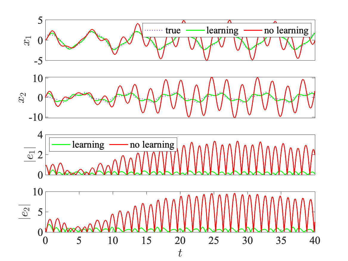
Figure 1: Comparison of state estimates and error norms with and without learning from data.

For fairness, we choose Legendre polynomials as basis functions and not monomials, which would perfectly fit the nonlinearity $\phi(q)$ with very few coefficients. Our basis functions are

$$\psi(\hat{q})=10\begin{bmatrix}(3\hat{q}_{1}^{2}-1)(3\hat{q}_{2}^{2}-1)\\ (3\hat{q}_{1}^{2}-1)\hat{q}_{2}\\ \hat{q}_{1}(3\hat{q}_{2}^{2}-1)\\ (5\hat{q}_{1}^{3}-3\hat{q}_{1})\\ (5\hat{q}_{2}^{3}-3\hat{q}_{2})\end{bmatrix},$$

where the scaling helps find good coefficients despite the strong bound on $\bar{p}_{\star}$. Performing Bayesian optimization with the GP-EI method using a weighting matrix $W_{1}=200$, $W_{2}=1$, and termination threshold $\varepsilon_{\sf EI}=0.01$ yields

$$p_{\infty}=10^{-3}\times\begin{bmatrix}-0.6077\\ 8.4930\\ -9.2877\\ 1.8897\\ 9.8417\end{bmatrix}$$

in $N=200$ training iterations, with $1000$ uniformly random samples on $[-\bar{p}_{\star},\bar{p}_{\star}]^{5}$ to select $p_{j}$ at each $j$ using (20). The surrogate GP model is constructed at each time using sklearn in Python or MATLAB’s fitrgp function in the Statistics and Machine Learning Toolbox. We use the Matérn ARD-52 kernel and select hyperparameters using BFGS on the log-likelihood function at each training iteration. The effects of model learning is illustrated in Figure 1. Prior to learning, the initial observer design provides bounded error dynamics (red continuous line), but the error is considerably reduced after learning is completed (green continuous line).

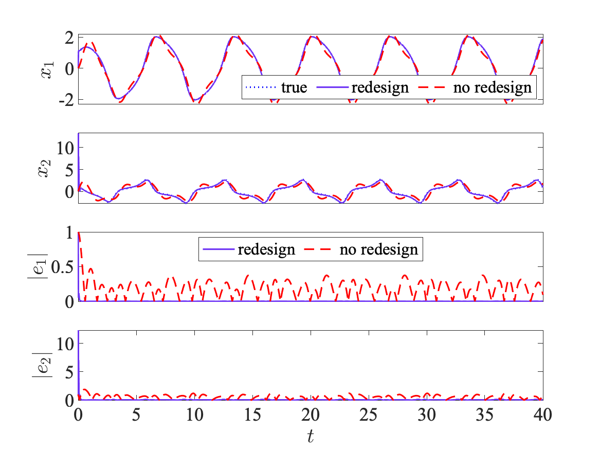
Figure 2: Comparison of state estimates and error norms with and without final redesign of the observer gains.

With the learned nonlinearity in a neural approximator/basis expansion form $p_{\infty}^{\top}\psi(\hat{q})$, we select $\mathbb{Q}=[-5,5]^{2}$ and use the kernelized Lipschitz estimation method in [27] to compute $\hat{\mathfrak{L}}_{\psi}=24.537$, with which we can solve (27) to get $L=\begin{bmatrix}39.3221&958.7488\end{bmatrix}^{\top}$. As seen from Figure 2, the redesign results in further reduction of state estimation error.

In order to demonstrate the effectiveness of the proposed algorithm, we compare the performance of our learning-based observer with well-known robust and adaptive observers in the literature. The observers we compare against include: the robust adaptive observer (RA) described in [28, Chapter 5], the high-gain (HG) observer described in [29], and the recurrent neural network (RNN) learning-based observer proposed in [30]. In all cases, we make multiple simplifications regarding knowledge of the model dynamics, since these observers failed to converge with completely unknown dynamics. In the first two observers, one requires a ‘nominal model’ for $\phi(q)$, which we assume to be $\hat{x}_{1}^{2}\hat{x}_{2}+0.2*\sin(\hat{x}_{2})$ to emulate a bounded disturbance on the model knowledge. For the neural observer, we start with an initial condition $\begin{bmatrix}0.5&0.5\end{bmatrix}^{\top}$ which is close to the true system state, because starting from the origin results in the neural approximator diverging. A comparison of the state estimation error in the unmeasured state, that is, $|e_{2}|$ is illustrated in Fig. 3. Clearly, our proposed observer (purple line) outperforms the others despite the simplifications made to help the other observer architectures. The RA observer (amber line) demonstrates good performance, but slow convergence rate, despite extensive hand-tuning - another drawback of this observer is that the observer state-space 8-dimensional and there are multiple hyperparameters and gains that need hand-tuning. The HG observer (green line), expectedly, has high state estimation error initially, although the steady-state estimation norm is smaller than RA and RNN, albeit larger than our proposed observer. Finally, the RNN observer (magenta line) exhibits significantly worse performance with time, and sometimes the estimation error grows large; this is because the observer estimation error dynamics are uniformly ultimately bounded, but not ISS, so large approximation errors in the recurrent neural network result in poor quality of the state estimates.

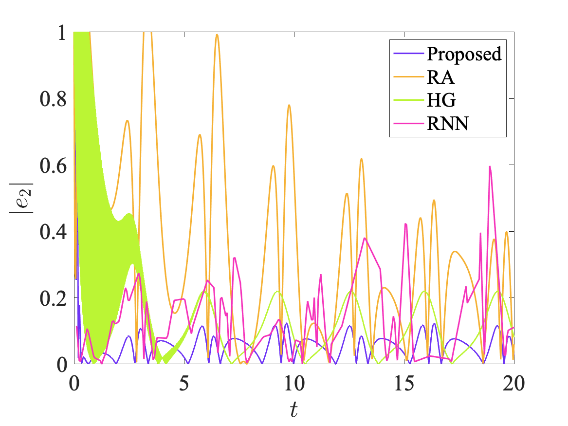
Figure 3: Comparative study of our proposed method with robust and adaptive observers in the literature. RA = Robust adaptive observer [28, Chapter 5], HG = High-gain observer [29], RNN = Recurrent neural network observer [30]. RA and HG have knowledge of the nonlinearity $\phi$, and RNN state is initialized near the system’s initial state.

7 Conclusions

In this paper, we provide a design methodology for constructing state estimators with unmodeled dynamics. We generate an initial observer that is robust to the learning error, in thes sense of ISS guarantees, and use this conservative initial state estimator to iteratively learn the unmodeled dynamics via Bayesian optimization in a purely data-driven manner. Once a suitable estimate of the complete model is achieved, based on an information measure, we redesign the observer using the learned dynamics to reduce conservatism. Furthermore, the proposed modular design, based on a model-based part ensuring the safety of the learning via ISS guarantees, added to a data-driven optimization part, allows us to plug-in any data-driven optimization approach with convergence guarantees, e.g. Bayesian optimization, extremum seekers, etc.

Further investigations will be conducted to deal with the case of output measurement noise, which can enter the system both at the observer feedback level or at the learning cost function measurement level.

Appendix: Implementation

Algorithm 1 Bayesian Learning-based Observer

1:Initial conditions $x_{0}$, $\hat{x}_{0}$

2:System matrices $A$, $B$, $C$

3:Function argument matrix $C_{q}$ $\triangleright$ default: $I$

4:Basis functions $\psi$

5:Initial coefficients $p_{0}$ $\triangleright$ default: 0

6:Upper bound on coefficients $\bar{p}_{\star}$ $\triangleright$ default: $10^{-3}$

7:Range of $\hat{\mathfrak{L}}_{\psi}$ to perform line search

8:Batch size for learning $T_{\ell}$

9:Cost function weights $W_{1},W_{2}$ $\triangleright$ p.s.d. matrices

10:Kernel $\mathcal{K}$ for GP regression $\triangleright$ default: Matérn 52

11:Termination threshold $\varepsilon_{\sf EI}$ $\triangleright$ default: $10^{-3}$

12: 

13:Initial L-ISS observer design

14: 

15:Select $A$ such that $(A,C)$ is observable

16:$\hat{\mathfrak{L}}_{\psi},L_{0}\leftarrow$ perform line search (14) $\triangleright$ involves solving SDP (10) for $L_{0}$ corresponding to $\hat{\mathfrak{L}}_{\psi}$

17:Parameterize initial observer (2) with $L_{0}$ and $p_{0}$

18: 

19:Safe learning from online data

20: 

21:for $j=0:N-1$ do

22:    Collect batch data (estimated states $\{\hat{x}\}$ and measurements $\{y\}$) from system

23:    $\mathcal{J}(p_{j})\leftarrow$ compute via (15)

24:    Learn surrogate GP model from data $\{p_{j},\mathcal{J}(p_{j})\}$

25:    $\mu,\sigma\leftarrow$ use GP to compute on samples drawn from $\mathbb{P}$

26:    $p_{j+1}\leftarrow$ obtain via expected improvement (20)

27:    Re-parameterize observer (2) with $L_{0}$ and $p_{t}\leftarrow p_{j+1}$

28:    Terminate if condition (21) holds

29:$p_{\infty}\leftarrow$ terminal value of $p_{j+1}$

30: 

31:Observer gain redesign

32: 

33:$L\leftarrow$ redesigned observer gain in (27)

34:Parameterize re-designed observer (25) with $L$ and $p_{\infty}$

References

- [1] Kumpati S Narendra and Kannan Parthasarathy. Identification and control of dynamical systems using neural networks. IEEE Transactions on Neural Networks, 1(1):4–27, 1990.
- [2] Elias B Kosmatopoulos, Marios M Polycarpou, Manolis A Christodoulou, and Petros A Ioannou. High-order neural network structures for identification of dynamical systems. IEEE Transactions on Neural Networks, 6(2):422–431, 1995.
- [3] Ankush Chakrabarty, Vu Dinh, Martin J Corless, Ann E Rundell, Stanisław H Żak, and Gregery T Buzzard. Support vector machine informed explicit nonlinear model predictive control using low-discrepancy sequences. IEEE Transactions on Automatic Control, 62(1):135–148, 2017.
- [4] Ján Drgoňa, Damien Picard, Michal Kvasnica, and Lieve Helsen. Approximate model predictive building control via machine learning. Applied Energy, 218:199–216, 2018.
- [5] Bahare Kiumarsi, Kyriakos G Vamvoudakis, Hamidreza Modares, and Frank L Lewis. Optimal and autonomous control using reinforcement learning: A survey. IEEE Transactions on Neural Networks and Learning Systems, 29(6):2042–2062, 2018.
- [6] Yuzhu Huang and Derong Liu. Neural-network-based optimal tracking control scheme for a class of unknown discrete-time nonlinear systems using iterative adp algorithm. Neurocomputing, 125:46–56, 2014.
- [7] J Theocharis and V Petridis. Neural network observer for induction motor control. IEEE Control Systems Magazine, 14(2):26–37, 1994.
- [8] Young H. Kim, Frank L. Lewis, and Chaouki T. Abdallah. A dynamic recurrent neural-network-based adaptive observer for a class of nonlinear systems. Automatica, 33(8):1539–1543, 1997.
- [9] Farzaneh Abdollahi, H.A. Talebi, and R.V. Patel. A Stable Neural Network-Based Observer With Application to Flexible-Joint Manipulators. IEEE Transactions on Neural Networks, 17(1):118–129, jan 2006.
- [10] Xin Liu, Chenguang Yang, Zhiguang Chen, Min Wang, and Chun Yi Su. Neuro-adaptive observer based control of flexible joint robot. Neurocomputing, 275:73–82, 2018.
- [11] Bhanu Pratap and Shubhi Purwar. Neural Network Observer for Twin Rotor MIMO System: An LMI Based Approach. In International Conference on Modeling, Identification and Control, pages 539–544, Okayama, Japan, 2010. IEEE.
- [12] Reihane Rahimilarki, Zhiwei Gao, Aihua Zhang, and Richard James Binns. Robust neural network fault estimation approach for nonlinear dynamic systems with applications to wind turbine systems. IEEE Transactions on Industrial Informatics, 3203(c):1–1, 2019.
- [13] Mouhacine Benosman and Jeff Borggaard. Robust nonlinear state estimation for a class of infinite-dimensional systems using reduced-order models. International Journal of Control, pages 1–12, 2019.
- [14] Shumon Koga, Mouhacine Benosman, and Jeff Borggaard. Learning-based robust observer design for coupled thermal and fluid systems. In 2019 American Control Conference (ACC), pages 941–946. IEEE, 2019.
- [15] A. Chakrabarty, A. Zemouche, R. Rajamani, and M. Benosman. Robust data-driven neuro-adaptive observers with lipschitz activation functions. In 2019 IEEE 58th Conference on Decision and Control (CDC), pages 2862–2867, 2019.
- [16] M. Benosman. Model-based vs. data-driven adaptive control: An overview. Journal of Adaptive Control and Signal Processing, 32(5):753–776, March 2018.
- [17] Jing Na, Guido Herrmann, and Kyriakos G Vamvoudakis. Adaptive optimal observer design via approximate dynamic programming. In 2017 American Control Conference (ACC), pages 3288–3293. IEEE, 2017.
- [18] A. Capone and S. Hirche. Interval observers for a class of nonlinear systems using gaussian process models. In 2019 18th European Control Conference (ECC), pages 1350–1355, 2019.
- [19] Ankush Chakrabarty and Martin Corless. Estimating unbounded unknown inputs in nonlinear systems. Automatica, 104:57–66, 2019.
- [20] Youssef N. Raffoul and Youssef M. Dib. Boundedness and Stability in Nonlinear Discrete Systems With Nonlinear Perturbation. Journal of Difference Equations and Applications, 9:853–862, 2003.
- [21] Boris Hanin. Universal function approximation by deep neural nets with bounded width and relu activations. Mathematics, 7(10):992, 2019.
- [22] Huijuan Li and Lars Grüne. Computation of local ISS Lyapunov functions for discrete-time systems via linear programming. Journal of Mathematical Analysis and Applications, 438(2):701–719, Jun 2016.
- [23] Andrii Mironchenko. Local input-to-state stability: Characterizations and counterexamples. Syst. Control Lett., 87:23–28, 2016.
- [24] Christopher KI Williams and Carl Edward Rasmussen. Gaussian Processes For Machine Learning. MIT press. Cambridge, MA, 2006.
- [25] Vu Nguyen, Sunil Gupta, Santu Rana, Cheng Li, and Svetha Venkatesh. Regret for expected improvement over the best-observed value and stopping condition. Journal of Machine Learning Research, 77:279–294, 2017.
- [26] V.K. Rohatgi. An Introduction to Probability Theory and Mathematical Statistics. John Wiley & Sons, 1976.
- [27] A. Chakrabarty, D. K. Jha, G. T. Buzzard, Y. Wang, and K. G. Vamvoudakis. Safe approximate dynamic programming via kernelized Lipschitz estimation. IEEE Transactions on Neural Networks and Learning Systems, pages 1–15, 2020.
- [28] Petros A Ioannou and Jing Sun. Robust adaptive control. Courier Corporation, 2012.
- [29] Hassan K Khalil and Laurent Praly. High-gain observers in nonlinear feedback control. International Journal of Robust and Nonlinear Control, 24(6):993–1015, 2014.
- [30] Bing Chen, Huaguang Zhang, Xiaoping Liu, and Chong Lin. Neural observer and adaptive neural control design for a class of nonlinear systems. IEEE Trans. on Neural Networks and Learning Systems, 29(9):4261–4271, 2017.