Energy-momentum conserving integration schemes for molecular dynamics

Abstract

We address the formulation and analysis of energy and momentum conserving time integration schemes in the context of particle dynamics, and in particular atomic systems. The article identifies three critical aspects of these models that demand a careful analysis when discretized: first, the treatment of periodic boundary conditions; second, the formulation of approximations of systems with three-body interaction forces; third, their extension to atomic systems with functional potentials. These issues, and in particular their interplay with Energy-Momentum integrators, are studied in detail. Novel expressions for these time integration schemes are proposed and numerical examples are given to illustrate their performance.

1 Introduction

Energy and momentum conserving algorithms are a frequently used class of structure preserving integration schemes [1, 2]. Their remarkable robustness and their good qualitative accuracy have made them popular choices for simulating the governing equations of particle dynamics [3, 4], nonlinear solid mechanics [5, 6], nonlinear shells and rods [7, 8, 9, 10], multibody dynamics [11, 12], gradient systems [13], and general PDEs [14].

Given the good properties of these methods, it is remarkable that they have not received more attention in the field of molecular dynamics, or in general, molecular thermodynamics. The governing equations of the latter are essentially Hamiltonian and fit seamlessly in the framework developed since the 70s for integrating this type of problems, while preserving the energy and the momenta. It would seem natural that integration schemes designed to preserve the main invariants of the motion would give accurate predictions of the thermodynamic averages, of interest in many practical and theoretical situations [15, 16, 17, 18], but have rarely been studied [19]. Instead, molecular dynamics codes seem to favor the use of the explicit Verlet method or symplectic methods. While the latter have good properties in terms of computational cost, accuracy, and geometry preservation, they lack energy conservation, a key invariant most important in the simulation of microcanonical ensembles. A thorough investigation of the accuracy of energy and momentum conserving schemes in capturing the statistical behavior of atomistic systems for long periods of simulation is lacking. Preliminary results [19] are promising, but much testing and validation is still required.

The development and implementation of energy and momentum conserving algorithms in the context of molecular dynamics has specific issues that affect the discretization of the equations and their analysis, issues that do not appear in their application to nonlinear solids, shells, rods, etc., or any of the other systems for which the use of these methods is widespread. The first critical issue is the treatment of periodic boundary conditions. These are almost invariably required for the study of average properties in particle systems [18, 20], and demand a careful analysis, especially to ascertain whether they spoil the conserving properties of the method or not. Taking this into account requires to consider the geometry and topology of the periodic configuration space, and might affect also the accuracy of the integration scheme.

The second issue that needs to be carefully dealt with is the use of conserving schemes in the context of three-body potentials. These functions are employed in modeling angle interactions in atomic bonding [21, 22], and their impact on the global behavior of some systems is so critical that needs to be accounted for. In fact, atomic systems with potentials of this type allow for large relative motions among the particles, and this is precisely the arena where conserving schemes have shown their superiority with regard to other implicit integrators.

The third aspect that requires a detailed analysis is the application of conserving schemes to mechanical systems in which the potential is based on cluster functionals [23, 24, 25, 26, 27]. These effective potentials are often required for the correct modeling of complex binding among metallic atoms and need again a careful study when used in combination with conserving schemes. While pair potentials of the Lennard-Jones type [28] have been employed together with Energy-Momentum conserving schemes [3], their formulation for cluster potentials needs to be specifically addressed.

In this article we formulate energy and momentum conserving schemes for the simulation of the dynamics of atomic systems. Some of the methods discussed have already been employed in the literature, and we identify new ones. In all cases, we explain how the three critical issues identified before (periodic boundary conditions, three-body potentials, functional potentials) affect their formulation since none of the three have been studied, to our knowledge, before.

The rest of the article has the following structure. In Section 2 we review the basic topology of periodic systems so as to clearly define the distance function. Section 3 introduces particle dynamics, with special attention to its Hamiltonian structure. Next, in Section 4, conserving time integration schemes are presented for particle systems in periodic domains, restricted to those with pair potentials. These are extended to systems with angle potentials in Section 5 and to atomic systems with functional potentials in Section 6. In the three cases of study, numerical simulations are provided to confirm the conservation properties of the fully discrete method. The article concludes in Section 7 with a summary of the main findings.

2 The topology of periodic domains

In this article we study the dynamic motion of systems of particles. This type of problems is of great importance for the simulation of matter at the atomic scale and a very large body of references study details pertaining to their numerical solution and the information that can be extracted from these simulations.

Many particle systems of interest are formulated in periodic domains. These allow to study large systems by only discretizing representative volumes, much smaller in size, while hopefully not losing too much information. In this section we gather some topological and geometrical facts of periodic domains that will be necessary to analyze numerical methods.

We start by considering a periodic three-dimensional box $\mathcal{B}$ of side length $L$, noting that all the results are applicable to systems in one and two dimensions, with the corresponding modifications. This box is isomorphic to the torus $\mathbb{T}^{3}$ (see e.g. [18, 16]), which itself can be identified with the product manifold $S^{1}\times S^{1}\times S^{1}$. Hence, each point $\boldsymbol{\xi}\in\mathbb{T}^{3}$ can be uniquely characterised by three angles $(\alpha,\beta,\gamma)$ and the complete manifold is covered by a single chart.

Numerical methods defined on $\mathbb{T}^{3}$ pose difficulties that can be alleviated by mapping this set into a more convenient one. For that, let us first define the following equivalence relation on $\mathbb{R}^{3}$: two points $\boldsymbol{x},\boldsymbol{y}\in\mathbb{R}^{3}$ are defined to be equivalent, and indicated as $\boldsymbol{x}\sim\boldsymbol{y}$, if there exists a triplet of integers $\boldsymbol{z}\in\mathbb{Z}^{3}$ such that $\boldsymbol{x}=\boldsymbol{y}+L\boldsymbol{z}$. Using this equivalence relation, we can define the quotient space $\mathbb{P}:=\mathbb{R}^{3}/\mathbb{Z}^{3}$ that is homeomorphic to the torus. In what follows the equivalent class of a point $\boldsymbol{x}\in\mathbb{R}^{3}$ will be denoted as $[\boldsymbol{x}]\in\mathbb{P}$.

When dealing with systems of particles in periodic domains one has to choose one of the two homeomorphic descriptions described above, namely, the torus and $\mathbb{P}$. From the computational point of view, employing the latter has many advantages. The first one is that given a distance on $\mathbb{R}^{3}$, this quotient space naturally inherits a distance, and thus a topology. In terms of the standard Euclidean distance $d(\cdot,\cdot):\mathbb{R}^{3}\times\mathbb{R}^{3}\to\mathbb{R}^{+}\cup\{0\}$ we can define $d_{T}(\cdot,\cdot):\mathbb{P}\times\mathbb{P}\to\mathbb{R}^{+}\cup\{0\}$ by the relation

$$d_{T}([\boldsymbol{x}],[\boldsymbol{y}])=\inf_{\boldsymbol{x}\in[\boldsymbol{x}],\boldsymbol{y}\in[\boldsymbol{y}]}d(\boldsymbol{x},\boldsymbol{y})\ .$$ (1)

Abusing slightly the notation, from this point we will write $d_{T}(\boldsymbol{x},\boldsymbol{y})$ instead of $d_{T}([\boldsymbol{x}],[\boldsymbol{y}])$.

The second advantage of such a choice is that, for each equivalent class $[\boldsymbol{x}]$, there exists a unique point $\bar{\boldsymbol{x}}\in[\boldsymbol{x}]\cap[-L/2,L/2)^{3}$ that serves as identifier of the whole class which, in practical terms, implies that all operations need to be performed as with standard points in a cubic box. This identifier can be found using a projection operator

$$\boldsymbol{\pi}:\mathbb{R}^{3}\to\mathcal{B}$$ (2)

defined as

$$\bar{x}_{j}=\pi(\boldsymbol{x})_{j}=x_{j}-\mathop{\mathtt{floor}}\left(\frac{x_{j}+L/2}{L}\right)L,$$ (3)

where $x_{j},j=1,2,3$ denote the Cartesian coordinates of the point $\boldsymbol{x}$ and $\mathop{\mathtt{floor}}:\mathbb{R}\to\mathbb{Z}$ is the function that gives the largest integer smaller than or equal to a given real number. See Figure 1 for an illustration of the projection operator.

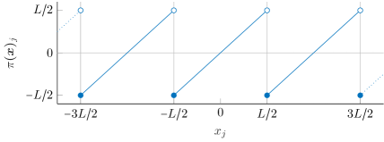
Figure 1: Graph of the projection operator $\boldsymbol{\pi}$ restricted to one of the three coordinates of Euclidean space.

The projection map $\boldsymbol{\pi}$ determines some of the properties and limitations of the numerical methods employed on systems with periodic boundary conditions, and it is helpful to summarize some of its properties:

1. $\boldsymbol{\pi}$ is a nonlinear, surjective, projection, that is $\boldsymbol{\pi}\circ\boldsymbol{\pi}=\boldsymbol{\pi}$.

2. The point $\boldsymbol{\pi}(\boldsymbol{x})$ is the closest one to the origin among all points in $[\boldsymbol{x}]$, that is,

   $$\boldsymbol{\pi}(\boldsymbol{x})=\arg\inf_{\boldsymbol{x}\in[\boldsymbol{x}]}d(\boldsymbol{x},\boldsymbol{0})$$ (4)

3. In general, for arbitrary $\boldsymbol{x},\boldsymbol{y}\in\mathbb{R}^{3}$,

   $$d_{T}(\boldsymbol{x},\boldsymbol{y})=\left|\boldsymbol{\pi}(\boldsymbol{x}-\boldsymbol{y})\right|\neq\left|\boldsymbol{\pi}(\boldsymbol{x})-\boldsymbol{\pi}(\boldsymbol{y})\right|.$$ (5)

4. The map $\boldsymbol{\pi}$ is $C^{\infty}$ except on the planes $x_{i}=L/2+k_{i}L$, with $k_{i}\in\mathbb{Z}$ and $i=1,2,3$, where it is discontinuous. Away from these planes, the gradient $\nabla\boldsymbol{\pi}$ is the identity $\boldsymbol{I}:\mathbb{R}^{3}\to\mathbb{R}^{3}$. A one-dimensional illustration of the gradient $\nabla\boldsymbol{\pi}$ is given in Figure 2.

   

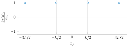
   Figure 2: Graph of the gradient of the projection operator $\nabla\boldsymbol{\pi}$ restricted to one of the three coordinates of Euclidean space.

5. For any $\boldsymbol{x}\in\mathbb{R}^{3}$

   $$\boldsymbol{\pi}(\boldsymbol{x})=-\boldsymbol{\pi}(-\boldsymbol{x})\ .$$ (6)

6. For any $\boldsymbol{x},\boldsymbol{y}\in\mathbb{R}^{3}$ and $\boldsymbol{a}\in\mathbb{R}^{3}$

   $$d_{T}(\boldsymbol{x}+{\boldsymbol{a}},\boldsymbol{y}+\boldsymbol{a})=d_{T}(\boldsymbol{x},\boldsymbol{y})\ .$$ (7)

   However, in general, if $\boldsymbol{Q}\in SO(3)$,

   $$d_{T}(\boldsymbol{x},\boldsymbol{y})\neq d_{T}(\boldsymbol{Q}\boldsymbol{x},\boldsymbol{Q}\boldsymbol{y})\ .$$ (8)

   Hence, in contrast with the Euclidean distance, the function $d_{T}(\cdot,\cdot)$ is not invariant under the action of the special orthogonal group.

3 Particle dynamics: basic description

In this section we provide the basic ingredients that describe the dynamics of particulate systems. This dynamical system is governed by Hamilton’s equations of motion, and most of its complexity comes from the particle interactions, as given by the potential energy. Here we present a fairly general class of potentials that will be examined more carefully in Sections 4, 5 and 6.

3.1 System description

Let us consider a system of $N$ particles labeled $a=1,2,\ldots,N$ moving inside a periodic box $\mathcal{B}$. Let the mass of the $a$-th particle be denoted as $m^{a}$, its position as $\boldsymbol{x}^{a}$, and its velocity as $\boldsymbol{v}^{a}=\dot{\boldsymbol{x}}^{a}$, where the dot indicates the derivative with respect to time.

A system of particles such as the one introduced possesses a kinetic energy defined by

$$T:=\sum_{a=1}^{N}\frac{1}{2}m^{a}|\boldsymbol{v}^{a}|^{2}\ ,$$ (9)

and a potential energy

$$V=\hat{V}(\{\boldsymbol{x}^{a}\}_{a=1}^{N})\ ,$$ (10)

modeling the energetic interactions among all the particles. This potential energy is always a model of the true interatomic interaction and as such there exists a large number of simple effective potentials that have proven their value in different contexts (gases, fluids, organic molecules, metals, etc.).

3.2 Equations of motion

The dynamics of systems of particles are governed by Hamilton’s equations of motion, namely,

$$\dot{{\boldsymbol{x}}}^{a}=\frac{1}{m^{a}}\boldsymbol{p}^{a}\ ,\qquad\dot{\boldsymbol{p}}^{a}=-\frac{\partial}{\partial{\boldsymbol{x}}^{a}}\hat{V}(\{\boldsymbol{x}^{b}\}_{b=1}^{N})\ ,$$ (11)

where $a=1,\ldots,N$, and $\boldsymbol{p}^{a}=m^{a}\boldsymbol{v}^{a}$ is the momentum of particle $a$. The gradient of the potential energy is related to the forces acting on the particles, and we define

$$\boldsymbol{f}^{a}:=-\frac{\partial}{\partial{\boldsymbol{x}}^{a}}\hat{V}(\{\boldsymbol{x}^{b}\}_{b=1}^{N})$$ (12)

to be the resultant of all forces applied on particle $a$.

These standard equations need to be carefully studied since the topology of $\mathcal{B}$ is not identical to that of Euclidean space and the notion of derivative has to be re-examined. For the moment being, let us assume that this object is well-defined, deferring until Section 4 a more detailed inspection.

3.3 Conserved quantities

Eqs. (11) describe the motion of systems of particles that often possess first integrals, that is, conserved quantities along their trajectories. These quantities are of great relevance to understand the qualitative dynamics of the system, to develop controls, etc. These momentum maps are related to the symmetries of the equations, according to Noether’s theorem (see e.g. [29]). We review them very briefly, since they have a direct impact in the formulation of conserving schemes.

We consider only potential energies with translational invariant, that is, functions $\hat{V}$ such that for every vector $\boldsymbol{c}\in\mathbb{R}^{3}$ satisfy

$$\hat{V}(\{\boldsymbol{x}^{a}\}_{a=1}^{N})=\hat{V}(\{\boldsymbol{x}^{a}+\boldsymbol{c}\}_{a=1}^{N})\ .$$ (13)

Differentiating both sides of this equation with respect to $\boldsymbol{c}$ and setting later $\boldsymbol{c}=\boldsymbol{0}$ we obtain the relation

$$\boldsymbol{0}=\sum_{a=1}^{N}\frac{\partial\hat{V}}{\partial\boldsymbol{x}^{a}}(\{\boldsymbol{x}^{b}\}_{b=1}^{N})=-\sum_{a=1}^{N}\boldsymbol{f}^{a}\ .$$ (14)

This invariance condition is related to the conservation of the linear momentum of the system, defined as

$$\boldsymbol{L}=\sum_{a=1}^{N}\boldsymbol{p}^{a}\ .$$ (15)

The time derivative of this quantity follows from the definition of particle momentum and eq. 14:

$$\dot{\boldsymbol{L}}=\sum_{a=1}^{N}\dot{\boldsymbol{p}}^{a}=\sum_{a=1}^{N}\boldsymbol{f}^{a}=\boldsymbol{0}\ .$$ (16)

Systems of particles moving in the Euclidean space $\mathbb{R}^{n}$, with $n=2$ or $3$, often conserve angular momentum. This is a consequence of the rotational invariance of the potential energy. However, systems defined on a periodic domain do not preserve it, in general (see e.g. [30, 31]). One way to explain this loss of symmetry is by noting that the projection (3) is not rotationally invariant (see eq. 8) and thus when used in the definition of the potential energy, it spoils the invariance of the whole system.

The total energy of the system is given as the sum of kinetic energy $T$ and potential energy $V$. The time derivative of the energy can be evaluated using the equations of motion (11), giving

$$\dot{E}=\sum_{a=1}^{N}m^{a}\boldsymbol{v}^{a}\cdot\dot{\boldsymbol{v}}^{a}-\sum_{a=1}^{N}\boldsymbol{f}^{a}\cdot\dot{\boldsymbol{x}}^{a}\\ =\sum_{a=1}^{N}\boldsymbol{f}^{a}\cdot\boldsymbol{v}^{a}-\sum_{a}^{N}\boldsymbol{f}^{a}\cdot\dot{\boldsymbol{x}}^{a}=0\ ,$$ (17)

proving that the total energy must be a first integral of the motion.

Given the relevance of the aforementioned conservation laws, numerical schemes have been proposed that attempt to preserve them. In particular, Energy-Momentum (EM) schemes, the ones under study in the present work, have been designed to integrate the equations of Hamiltonian systems while preserving both linear and angular momentum, in addition to the total energy. From the previous discussion, however, it follows that when dealing with periodic systems, one might focus on the preservation of the linear momentum and energy, only.

3.4 The hierarchical definition of the potential energy

The potential energy of a system of particles is a function with the general form given in eq. 10 satisfying the invariance condition (13). A hierarchy of functions of growing complexity can be defined considering interactions involving an increasing number of particles. This is abstractly expressed as

$$V=V_{0}+\sum_{\begin{subarray}{c}a,b=1\\ a\neq b\end{subarray}}^{N}V_{2}(\boldsymbol{x}_{a},\boldsymbol{x}_{b})+\sum_{\begin{subarray}{c}a,b,c=1\\ a\neq b\neq c\end{subarray}}^{N}V_{3}(\boldsymbol{x}_{a},\boldsymbol{x}_{b},\boldsymbol{x}_{c})+\ldots,$$ (18)

where $V_{k}$ is a function involving $k-$tuples of atoms and satisfying eq. 13. The formulation of accurate potentials is an active field of research and we limit our exposition to the most common types. The reader may consult standard references for a detailed motivation and derivation of other types (e.g. [27]).

A convenient way of formulating potential functions that are translationally invariant is to include atomic interactions only via the distance between pairs of particles. In general, this would mean that the functions $V_{k}$ employed in eq. 18 must be of the form

$$\begin{split}V_{2}(\boldsymbol{x}_{a},\boldsymbol{x}_{b})&=\tilde{V}_{2}(d(\boldsymbol{x}_{a},\boldsymbol{x}_{b}))\ ,\\ V_{3}(\boldsymbol{x}_{a},\boldsymbol{x}_{b},\boldsymbol{x}_{c})&=\tilde{V}_{3}(d(\boldsymbol{x}_{a},\boldsymbol{x}_{b}),d(\boldsymbol{x}_{b},\boldsymbol{x}_{c}),d(\boldsymbol{x}_{c},\boldsymbol{x}_{a}))\ ,\end{split}$$ (19)

and similarly for higher order terms.

3.5 Dynamics in periodic domains

Eqs. (11) define the motion of particles in periodic domains, but special care has to be taken with the definition of the potential energy and its derivative.

With respect to the potential, we note that when formulating the dynamics of particles in periodic domains the distance function $d(\cdot,\cdot)$ in eq. 19 should be replaced with the distance $d_{T}(\cdot,\cdot)$ defined in eq. 1.

An aspect with important practical implications is that hierarchical potential functions of the form (18) are invariably defined employing a cut-off radius that effectively limits the number of particles that interact with those within that distance, in the sense of $d_{T}(\cdot,\cdot)$. Moreover, in order to avoid the singularities in the definition of the gradient of this distance, the cut-off radius is always chosen to be strictly smaller than $L/2$ (see Figure 2). Equivalently, the dimension $L$ of the periodic box must be selected larger than twice the cut-off radius. Under this condition, we observe that a collection of $N$ particles in a periodic box $\mathcal{B}$ is a mathematical representation of an infinite domain consisting of boxes of dimension $L\times L\times L$ that repeat themselves in the three directions of space.

The formulation of energy and momentum conserving schemes in this kind of domains must take these two remarks into consideration, and we explore them in the following sections, starting from the simplest potential function possible.

4 Energy-Momentum methods for periodic systems with pairwise interactions

In this section we study the formulation of energy and momentum conserving algorithms for systems of particles in periodic domains where the potential energy includes only pairwise interactions. In terms of practical applications, only the simplest potentials belong to this class (for example, Lennard-Jones’). They are only accurate for modeling noble gases, but are very often employed for benchmarking and the study of numerical methods.

4.1 Equations of motion

We consider again a system of $N$ particles in a periodic box $\mathcal{B}$ of side $L$ with equations of motion (11) and an effective potential

$$V=\frac{1}{2}\sum_{\begin{subarray}{c}a,b=1\\ b\neq a\end{subarray}}^{N}\tilde{V}\left(d_{T}({\boldsymbol{x}}^{a},{\boldsymbol{x}}^{b})\right),$$ (20)

where $\tilde{V}:\mathbb{R}^{+}\cup\{0\}\to\mathbb{R}$. Using the definitions

$$\bar{\boldsymbol{r}}^{ab}:=\boldsymbol{\pi}(\boldsymbol{x}^{b}-\boldsymbol{x}^{a})\qquad\mathrm{and}\qquad\bar{r}^{ab}=d_{T}(\boldsymbol{x}^{a},\boldsymbol{x}^{b}):=|\bar{\boldsymbol{r}}^{ab}|\ ,$$ (21)

the forces (12) deriving from a pairwise potential can be written as

$$\boldsymbol{f}^{a}=\sum_{\begin{subarray}{c}b=1\\ a\neq b\end{subarray}}^{N}\boldsymbol{f}^{ab}\ ,\qquad\mathrm{with}\qquad\boldsymbol{f}^{ab}=\tilde{V}^{\prime}(\bar{r}^{ab})\frac{\bar{\boldsymbol{r}}^{ab}}{\bar{r}^{ab}}\ .$$ (22)

For the following sections we further define

$${\boldsymbol{r}}^{ab}:=\boldsymbol{x}^{b}-\boldsymbol{x}^{a}\qquad\mathrm{and}\qquad{r}^{ab}=d(\boldsymbol{x}^{a},\boldsymbol{x}^{b})=|{\boldsymbol{r}}^{ab}|\ .$$ (23)

4.2 Time discretization

We consider now the integration in time of the equations of motion (11) of a system in the periodic box $\mathcal{B}$ and effective potential (20). To approximate their solution we will employ implicit time stepping schemes that partition the integration interval $[0,T]$ into disjoint subintervals $[t_{n},t_{n+1}]$ with $t_{n}=n\Delta t$, and $\Delta t$ being the time step size, assumed to be constant to simplify the notation. In the algorithms defined below, we will use the notation $\boldsymbol{x}_{n}$ to denote the approximation to $\boldsymbol{x}(t_{n})$, and similarly for the velocity. Moreover, the symbol $f_{n+\alpha}$ will denote the convex combination $(1-\alpha)f_{n}+\alpha f_{n+1}$ for any variable $f$ and $0\leq\alpha\leq 1$.

4.2.1 Midpoint scheme

The canonical midpoint rule approximates the equations of motion (11) by the implicit formula

$$\frac{\boldsymbol{x}^{a}_{n+1}-\boldsymbol{x}^{a}_{n}}{\Delta t}=\boldsymbol{v}^{a}_{n+1/2},\qquad m^{a}\frac{\boldsymbol{v}^{a}_{n+1}-\boldsymbol{v}^{a}_{n}}{\Delta t}=\sum_{\begin{subarray}{c}b=1\\ a\neq b\end{subarray}}^{N}\boldsymbol{f}_{MP}^{ab}\ .$$ (24)

Here we introduced $\boldsymbol{f}^{ab}_{MP}$, the midpoint approximation of the force acting on particle $a$ due to the presence of particle $b$, that is,

$$\boldsymbol{f}_{MP}^{ab}:=\tilde{V}^{\prime}(\bar{r}^{ab}_{n+1/2})\frac{\bar{\boldsymbol{r}}^{ab}_{n+1/2}}{|\bar{\boldsymbol{r}}^{ab}_{n+1/2}|}\ ,$$ (25)

with

$$\bar{\boldsymbol{r}}^{ab}_{n+1/2}=\boldsymbol{\pi}(\boldsymbol{x}^{b}_{n+1/2}-\boldsymbol{x}^{a}_{n+1/2})\ ,\qquad\bar{r}^{ab}_{n+1/2}=d_{T}(\boldsymbol{x}^{a}_{n+1/2},\boldsymbol{x}^{b}_{n+1/2}).$$ (26)

As in the continuous case, the condition

$$\boldsymbol{f}_{MP}^{ab}=-\boldsymbol{f}_{MP}^{ba}$$ (27)

holds due to eq. 6. The properties of the midpoint rule are well known. For example, this method preserves the total liner momentum of the system, defined at an instant $t_{n}$ as

$$\boldsymbol{L}_{n}=\sum_{a=1}^{N}m^{a}\boldsymbol{v}_{n}^{a}\ .$$ (28)

To prove this property it suffices to verify

$$\frac{\boldsymbol{L}_{n+1}-\boldsymbol{L}_{n}}{\Delta t}=\sum_{a=1}^{N}m^{a}\frac{\boldsymbol{v}_{n+1}^{a}-\boldsymbol{v}_{n}^{a}}{\Delta t}=\sum_{\begin{subarray}{c}a,b=1\\ a\neq b\end{subarray}}^{N}\boldsymbol{f}_{MP}^{ab}=\boldsymbol{0}\ ,$$ (29)

where we have employed eq. 27.

4.2.2 Energy and momentum conserving discretization

It is possible to construct a perturbation of the midpoint rule that, in addition to preserving the linear momentum of the system, preserves its total energy. The key ingredient of such methods is the so called discrete gradient operator, an approximation to the gradient that guarantees the strict conservation of energy and momentum along the discrete trajectories generated by the integrator.

Conserving integrators for problems in molecular dynamics have been studied since the 1970’s [4, 3, 32], although never for systems with periodic boundary conditions, with the exception of [19]. In all of these works, the conserving schemes are variations of the midpoint rule (24) of the form

$$\frac{\boldsymbol{x}^{a}_{n+1}-\boldsymbol{x}^{a}_{n}}{\Delta t}=\boldsymbol{v}^{a}_{n+1/2},\qquad m^{a}\frac{\boldsymbol{v}^{a}_{n+1}-\boldsymbol{v}^{a}_{n}}{\Delta t}=-\mathsf{D}_{\boldsymbol{x}^{a}}V,$$ (30)

where $\mathsf{D}_{\boldsymbol{x}^{a}}$ is precisely the discrete gradient operator, an algorithmic approximation to the derivative $\frac{\partial}{\partial\boldsymbol{x}^{a}}$. In analogy to expression (25), the discrete gradient defines a force contribution, to be specified later, such that

$$\mathsf{D}_{\boldsymbol{x}^{a}}V=-\sum_{\begin{subarray}{c}b=1\\ a\neq b\end{subarray}}^{N}\boldsymbol{f}_{algo}^{ab}\ .$$ (31)

If the following condition holds

$$\boldsymbol{f}^{ab}_{algo}=\boldsymbol{f}_{MP}^{ab}+\mathcal{O}(\Delta t^{2})\ ,$$ (32)

the second order accuracy of the midpoint rule will be preserved. If we want the new method to preserve linear momentum we note from the previous section that it suffices that the pairwise forces $\boldsymbol{f}^{ab}_{algo}$ mimic the symmetry condition (27), that is,

$$\boldsymbol{f}^{ab}_{algo}=-\boldsymbol{f}^{ba}_{algo}\ .$$ (33)

Any second order perturbation of $\boldsymbol{f}_{MP}^{ab}$ with this property will result in a second order accurate integrator that preserves linear momentum. The “classical” EM method is constructed in such a way, and preserves, in addition to the total energy, the linear and angular momenta of the system, the latter being important in domains without periodic boundary conditions [32].

For problems in molecular dynamics interacting through pair potentials and posed on periodic domains, the “classical” EM method is based on the discrete gradient (31) with

$$\boldsymbol{f}^{ab}_{algo}=\boldsymbol{f}^{ab}_{algo}(\boldsymbol{r}_{n}^{ab},\boldsymbol{r}_{n+1}^{ab}):=\frac{\tilde{V}^{ab}_{n+1}-\tilde{V}^{ab}_{n}}{\bar{r}^{ab}_{n+1}-\bar{r}^{ab}_{n}}\frac{\bar{\boldsymbol{r}}^{ab}_{n+1}+\bar{\boldsymbol{r}}^{ab}_{n}}{\bar{r}^{ab}_{n+1}+\bar{r}^{ab}_{n}}\ ,$$ (34)

where we have introduced the notation

$$\tilde{V}_{n}^{ab}=\tilde{V}(\bar{r}^{ab}_{n})\ ,$$ (35)

and where the appropriate limit must be taken in eq. 34 when $|\bar{r}^{ab}_{n+1}-\bar{r}^{ab}_{n}|\to 0$. This form of the discrete gradient is frequently cited in the literature of integration algorithms (see e.g. [19]) and is responsible for the conservation properties of the method, also in periodic domains. However, it is not the only possible form and, in fact, it can be shown that there are an infinite number of discrete gradients [33], some of which can be more easily extended to the periodic case.

More precisely, a second class of EM schemes follows from a new definition of the algorithmic approximation of the pairwise forces:

$$\boldsymbol{f}^{ab}_{algo}(\boldsymbol{r}_{n}^{ab},\boldsymbol{r}_{n+1}^{ab}):=\boldsymbol{f}_{MP}^{ab}+\frac{\tilde{V}^{ab}_{n+1}-\tilde{V}^{ab}_{n}+\boldsymbol{f}_{MP}^{ab}\cdot({\boldsymbol{r}}^{ab}_{n+1}-{\boldsymbol{r}}^{ab}_{n})}{|{\boldsymbol{r}}^{ab}_{n+1}-{\boldsymbol{r}}^{ab}_{n}|}\;\boldsymbol{n},$$ (36)

where $\boldsymbol{n}$ is the normalized direction given by

$$\boldsymbol{n}=\frac{{\boldsymbol{r}}^{ab}_{n+1}-{\boldsymbol{r}}^{ab}_{n}}{|{\boldsymbol{r}}^{ab}_{n+1}-{\boldsymbol{r}}^{ab}_{n}|}\ .$$ (37)

This definition corrects the pairwise force between the particles $a$ and $b$ with a “small” term in the direction $\boldsymbol{n}$ depending on unprojected relative positions. This is the result of the fact that the first equation in (30) is not posed in the quotient space but rather in the full $\mathbb{R}^{3}$. It might be argued that such a correction is nonphysical because it is not defined on the quotient space, where the problem is posed. While this is true, the velocity equation is not posed on this space from the outset, and the proposed correction results from this mismatch.

The EM force given in eq. 36 is symmetric in $a$ and $b$. Hence, the method defined by (30) and (36) preserves linear momentum. To show that the method indeed preserves exactly the total energy exactly, it suffices to take the dot product of the (30)₁ with the left hand side of (30)₂, and vice versa, and then add the result over all particles, that is,

$$\sum_{a=1}^{N}m^{a}\frac{\boldsymbol{x}^{a}_{n+1}-\boldsymbol{x}^{a}_{n}}{\Delta t}\cdot\frac{\boldsymbol{v}^{a}_{n+1}-\boldsymbol{v}^{a}_{n}}{\Delta t} =\sum_{a=1}^{N}m^{a}\boldsymbol{v}^{a}_{n+1/2}\cdot\frac{\boldsymbol{v}^{a}_{n+1}-\boldsymbol{v}^{a}_{n}}{\Delta t}$$ (38)

$$\sum_{a=1}^{N}m^{a}\frac{\boldsymbol{v}^{a}_{n+1}-\boldsymbol{v}^{a}_{n}}{\Delta t}\cdot\frac{\boldsymbol{x}^{a}_{n+1}-\boldsymbol{x}^{a}_{n}}{\Delta t} =\sum^{N}_{\begin{subarray}{c}a,b=1\\ a\neq b\end{subarray}}\boldsymbol{f}^{ab}_{algo}\cdot\frac{\boldsymbol{x}^{a}_{n+1}-\boldsymbol{x}^{a}_{n}}{\Delta t}\ .$$

Subtracting (38)₂ from (38)₁ gives

$$\frac{T_{n+1}-T_{n}}{\Delta t}-\sum_{\begin{subarray}{c}a,b=1\\ a\neq b\end{subarray}}^{N}\boldsymbol{f}^{ab}_{algo}\cdot\frac{\boldsymbol{x}^{a}_{n+1}-\boldsymbol{x}^{a}_{n}}{\Delta t}=0\ ,$$ (39)

where the total discrete kinetic energy at time $t_{n}$ is given by

$$T_{n}=\sum_{a=1}^{N}\frac{1}{2}m^{a}\boldsymbol{v}^{a}_{n}\cdot\boldsymbol{v}^{a}_{n}\ .$$ (40)

In the spirit of eq. 36, further rewriting results in

$$\sum_{\begin{subarray}{c}a,b=1\\ a\neq b\end{subarray}}^{N}\boldsymbol{f}_{algo}^{ab}\cdot\frac{\boldsymbol{x}^{a}_{n+1}-\boldsymbol{x}^{a}_{n}}{\Delta t} =\frac{1}{\Delta t}\sum_{\begin{subarray}{c}a,b=1\\ a<b\end{subarray}}^{N}\boldsymbol{f}^{ab}_{algo}\cdot(\boldsymbol{x}^{a}_{n+1}-\boldsymbol{x}^{a}_{n}-\boldsymbol{x}^{b}_{n+1}+\boldsymbol{x}^{b}_{n})$$ (41)

$$=-\frac{1}{\Delta t}\sum_{\begin{subarray}{c}a,b=1\\ a<b\end{subarray}}^{N}\boldsymbol{f}_{algo}^{ab}\cdot(\boldsymbol{r}^{ab}_{n+1}-\boldsymbol{r}^{ab}_{n})\ .$$

Therefore, a necessary and sufficient condition for energy conservation is that the following directionality condition is satisfied

$$\sum^{N}_{\begin{subarray}{c}a,b=1\\ a<b\end{subarray}}\boldsymbol{f}^{ab}_{algo}\cdot(\boldsymbol{r}^{ab}_{n+1}-\boldsymbol{r}^{ab}_{n})=\frac{1}{2}\sum^{N}_{\begin{subarray}{c}a,b=1\\ a\neq b\end{subarray}}\left(\tilde{V}(\bar{r}^{ab}_{n+1})-\tilde{V}(\bar{r}^{ab}_{n})\right)\ .$$ (42)

It is important to emphasize that the proof is based on the inner product between the algorithmic EM force and the unprojected relative position vectors. Finally, to show that the EM scheme (36) is indeed a second-order accurate method it suffices to prove that the correction term in the definition (36) is of size $\mathcal{O}(\Delta t^{2})$. Making use of the relation

$$\boldsymbol{f}^{ab}_{MP}=-\frac{\partial\tilde{V}(|\bar{\boldsymbol{r}}^{ab}_{n+1/2}|)}{\partial\boldsymbol{x}^{a}}=\frac{\partial\tilde{V}(|\bar{\boldsymbol{r}}^{ab}_{n+1/2}|)}{\partial\boldsymbol{r}^{ab}}\ ,$$ (43)

a Taylor series expansion around the point $\boldsymbol{r}^{ab}_{n+1/2}$ gives

$$\tilde{V}^{ab}_{n+1}-\tilde{V}^{ab}_{n}=\boldsymbol{f}^{ab}_{MP}\cdot(\boldsymbol{r}^{ab}_{n+1}-\boldsymbol{r}^{ab}_{n})+\mathcal{O}(\Delta t^{3})\ .$$ (44)

Then, since the direction vector of the correction has size

$$\frac{{\boldsymbol{r}}^{ab}_{n+1}-{\boldsymbol{r}}^{ab}_{n}}{|{\boldsymbol{r}}^{ab}_{n+1}-{\boldsymbol{r}}^{ab}_{n}|}=\mathcal{O}(1)\ ,$$ (45)

and $|{\boldsymbol{r}}^{ab}_{n+1}-{\boldsymbol{r}}^{ab}_{n}|$ is $\mathcal{O}(\Delta t)$, we conclude that the correction term is indeed $\mathcal{O}(\Delta t^{2})$.

4.2.3 Time reversibility

Time-reversible (or symmetric) integration schemes are often favored for the approximation of Hamiltonian systems for two main reasons. First, the Hamiltonian flow itself is symmetric, so it is desirable that its numerical approximation also possesses this property. Second, symmetric numerical schemes are known to have several favorable properties [1], especially in long-term simulations. The class of EM integration schemes defined in this section have also this property. This is a direct consequence of the time-reversibility of the algorithmic approximation of the pairwise forces, namely,

$$\boldsymbol{f}^{ab}_{algo}(\boldsymbol{r}_{n}^{ab},\boldsymbol{r}_{n+1}^{ab})=\boldsymbol{f}^{ab}_{algo}(\boldsymbol{r}_{n+1}^{ab},\boldsymbol{r}_{n}^{ab}),$$ (46)

that is trivially satisfied by both (34) and (36).

4.3 Interatomic potential

For the following numerical examples we consider the well-known Lennard-Jones potential [28] with $r=\bar{r}^{ab}$, that is,

$$\tilde{V}(r)=4\epsilon\left[\left(\frac{\sigma}{r}\right)^{12}-\left(\frac{\sigma}{r}\right)^{6}\right]\ ,$$ (47)

where $\epsilon$ and $\sigma$ are constants.

4.3.1 Cut-off distance considerations

In the Lennard-Jones potential, atomic interactions between distant particles are negligible. For this reason, a cut-off distance $r_{c}$ is often introduced beyond which the interaction is completely ignored (see e.g. [18, 16]). However, simply trimming the Lennard-Jones potential beyond the cut-off distance leads to a discontinuity in this function at $r=r_{c}$ that might affect the properties of the integration scheme. Since the derivative of the potential enters the equations of motion (11), this discontinuity precludes the computation of the interatomic force at $r=r_{c}$. The discontinuity can be avoided, first, by shifting the potential function by the amount $V(r_{c})$, leading to the shifted potential (SP)

$$\tilde{V}_{\textrm{SP}}\left(r\right)=\begin{cases}V(r)-V(r_{c})&\text{if}\ r<r_{c}\ ,\\ 0&\text{if}\ r\geq r_{c}\ .\end{cases}$$ (48)

The derivative of this function at $r=r_{c}$ is still not defined and neither is the force. To resolve this physical inconsistency one can introduce a shifted and linearly truncated potential (SF), which is equivalent to a shift in the force (see e.g. [18, 31]), and given by

$$\tilde{V}_{\textrm{SF}}\left(r\right)=\begin{cases}V(r)-V(r_{c})-(r-r_{c})V^{\prime}(r_{c})&\text{if}\ r<r_{c}\ ,\\ 0&\text{if}\ r\geq r_{c}\ .\end{cases}$$ (49)

One can further introduce a quadratic correction term that yields the shifted and quadratically truncated potential (STF), which is equivalent to a shift and a linear truncation in the force,

$$\tilde{V}_{\textrm{STF}}\left(r\right)=\begin{cases}V(r)-V(r_{c})-(r-r_{c})V^{\prime}(r_{c})-\frac{1}{2}(r-r_{c})^{2}V^{\prime\prime}(r_{c})&\text{if}\ r<r_{c}\ ,\\ 0&\text{if}\ r\geq r_{c}\ .\end{cases}$$ (50)

This potential is twice differentiable. Due to its higher smoothness, it is better suited for structure-preserving schemes than the standard potential since it eliminates numerical oscillations in the energy evolution that sometimes appear when employing non-smooth potentials. As mentioned in Section 3.5, it is important to stress out that the cut-off distance must not be greater than $L/2$ for consistency with the minimum image convention. Due to the quadratic term in the corrected potential, a cut-off radius of $r_{c}=5\sigma$ is suggested.

4.4 Numerical evaluation

All numerical examples are based on a set of dimensionless units.

4.4.1 Accuracy study

In the first numerical example, we consider a two-dimensional box $[-L/2,L/2]^{2}$ with two particles. The initial positions and velocities are given, respectively, by

$$\boldsymbol{x}^{1} =(0,0)^{T},\quad \boldsymbol{v}^{1}=(0,0)^{T}\ ,$$

$$\boldsymbol{x}^{2} =(1.9,1)^{T},\quad \boldsymbol{v}^{2}=(5,0)^{T}\ ,$$

where the first particle is constrained to remain on the center of the box and only the second particle is allowed to move freely. For this simulation we used the Lennard-Jones potential with a simple spherical cut-off distance of $r_{c}=2.5\sigma$. The numerical values of the remaining parameters of the simulation can be found in Table 1.

Table 1: Accuracy study: Data used in the simulation

Material parameters	$\epsilon$	20	Final configuration
	$\sigma$	1	and trajectory
Mass	$m^{a}$	0.06
Side length	$L$	12
Newton tolerance	-	10-6
Simulation duration	$T$	0.8
Reference time step size	$\Delta t_{\text{ref}}$	0.0005
Time step size	$\Delta t$	0.004, 0.005,
		0.00625, 0.008,
		0.01, 0.125,
		0.016, 0.02,
		0.025

We first perform an accuracy analysis of the previously presented integrators and we compare them to the midpoint rule. These simulations are performed using ten different time step sizes for each integrator. Then we study the relative errors in the position and linear momentum, using as reference the midpoint rule solution, and defined respectively as

$$\textrm{e}^{(MP)}_{x}=\frac{||\boldsymbol{x}^{a}-\boldsymbol{x}^{a}_{r}||_{2}}{||\boldsymbol{x}^{a}_{r}||_{2}},\quad\textrm{e}^{(MP)}_{\textrm{p}}=\frac{||\boldsymbol{p}^{a}-\boldsymbol{p}^{a}_{r}||_{2}}{||\boldsymbol{p}^{a}_{r}||_{2}},$$ (51)

where $\square^{a}_{r}$, with $\square\in\{\boldsymbol{x},\boldsymbol{p}\}$, is the solution at time $T$ calculated with the midpoint, using the reference time step size $\Delta t_{\text{ref}}$, and where $\square^{a}$ is the solution of the considered scheme at time $T$ for each time step size $\Delta t$. Figures 3 and 4 confirm that all the schemes under consideration are second order accurate.

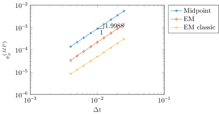
Figure 3: Accuracy study: Relative error in the position w.r.t midpoint rule

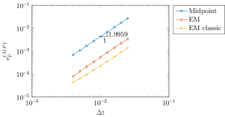
Figure 4: Accuracy study: Relative error in the linear momentum w.r.t midpoint rule

4.4.2 Energy consistency study

The second numerical example investigates the energy conservation properties of the integrators described in Section 4. We consider 150 arbitrarily positioned particles inside a three-dimensional periodic box $[-L/2,L/2]^{3}$ such that the initial distance between the particles is greater than $2^{1/6}\sigma$. Starting from rest, the kinetic energy of the system will rise until the system is in equilibrium due to the random order of the particles. For this simulation, we consider the shifted and quadratically truncated Lennard-Jones potential (STF) with a spherical cut-off distance of $r_{c}=5\sigma$. Numerical values for the parameters of the simulation can be found in Table 2.

Table 2: Energy consistency study: Data used in the simulation

Material parameters	$\epsilon$	2	Initial configuration
	$\sigma$	1
Mass	$m^{a}$	1
Sidelength	$L$	12
Newton tolerance	-	10-9
Simulation duration	$T$	40
Time steps	$\Delta t$	0.08

For this relatively large time step size, the midpoint rule introduces energy into the system leading to an energy blow-up and eventually to a termination of the simulation indicated with a vertical line in Figure 5.

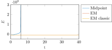
Figure 5: Energy consistency study: Total energy

Both EM methods described, on the other hand, preserve the total energy up to machine precision for the whole duration of the simulation. See Figure 6.

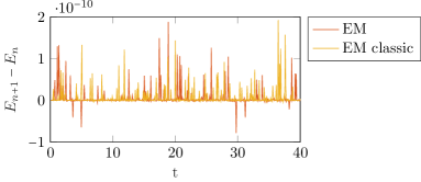
Figure 6: Energy consistency study: Total energy difference

Figure 7 shows the evolution of the kinetic energy throughout the simulation. Since this energy is proportional to the temperature in the system, the figure reveals that only the EM methods can compute the evolution of the system until it reaches equilibrium, for the chosen time step size.

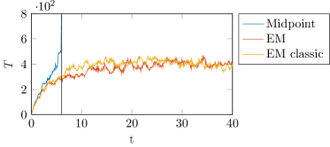
Figure 7: Energy consistency study: Kinetic energy

We compare the newly proposed EM method with an explicit integrator, namely, the velocity-Verlet scheme provided by the molecular dynamics code LAMMPS[34]. For this example we use the shifted and linearly truncated potential (SF) instead of the shifted and quadratically truncated potential (STF), since the former is available in the software package. Moreover, we extended the simulation duration to $T=80$.

Keeping the time step size of the EM method $\Delta t_{\textrm{EM}}=0.08$ constant, the time step size of the velocity-Verlet integrator $\Delta t_{\textrm{vV}}$ is reduced until the energy fluctuations become sufficiently small. As Figure 8 reveals, the time step size employed for the explicit method is $\Delta t_{\textrm{vV}}=0.0008$, 100 times smaller than the time step size of the EM method. This is the time step size required to keep the relative energy fluctuations in the explicit solution approximately below $0.1\permil$.

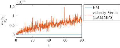
Figure 8: Energy consistency study: Relative energy drift for $\Delta t_{\textrm{EM}}=100\Delta t_{\textrm{vV}}$

Regarding the computational cost per step, the proposed implicit integrator naturally much more expensive that the explicit scheme. In order to do a fair comparison, however, the implementation of the EM method should be optimized similarly to LAMMPS, but this is not the focus of the present work.

In addition to the previous investigation, we perform an accuracy comparison between the EM and the velocity-Verlet methods. We use again the system described in Table 2 and obtain a reference solution with the explicit method and a small time step $\Delta t_{\textrm{ref}}=0.000001$. The displacement and momentum error measures of eq. (51) will be used to compare the accuracy of the two integrators for the time step sizes $\Delta t=\{$0.0001, 0.0002, 0.00025, 0.0004, 0.0005, 0.00625, 0.001, 0.0025, 0.004, 0.005, 0.01$\}$ and a final simulation time $T=4$. As shown in Figures 9 and 10, both schemes are second order accurate in the position and the linear momentum.

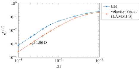
Figure 9: Energy consistency study: Relative error in the position w.r.t velocity-Verlet scheme (LAMMPS)

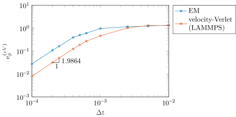
Figure 10: Energy consistency study: Relative error in the momentum w.r.t velocity-Verlet scheme (LAMMPS)

5 Energy-Momentum methods for periodic systems with three-body interactions

In Section 4 we derived the equation of motion of a system of $N$ particles moving inside a period box $\mathcal{B}$ where the interactions were based on pair potentials. For materials with strong covalent-bonding character, however, we further need to incorporate a bond-angle dependency to the effective potential. This can be archived by including three-body terms in the expression of the potential.

5.1 Equation of motion

We consider now a system of $N$ particles in a periodic box $\mathcal{B}$ of side $L$ with equations of motion (11) and an effective potential that depends only on the interactions among all triplets of particles. Such a potential must be of the form

$$V=\frac{1}{3!}\sum_{\begin{subarray}{c}a,b,c=1\\ a\neq b\neq c\end{subarray}}^{N}\tilde{V}\left(d_{T}({\boldsymbol{x}}^{a},{\boldsymbol{x}}^{b}),d_{T}({\boldsymbol{x}}^{a},{\boldsymbol{x}}^{c}),d_{T}({\boldsymbol{x}}^{b},{\boldsymbol{x}}^{c})\right)\ ,$$ (52)

where $\tilde{V}:\mathbb{R}^{+}\cup\{0\}\times\mathbb{R}^{+}\cup\{0\}\times\mathbb{R}^{+}\cup\{0\}\to\mathbb{R}$ is a three-body potential between the $a$-th, $b$-th, and the $c$-th particle. The total kinetic energy of the system is given by eq. 9. The forces acting on the particles defined by eq. 12 can be written using the definitions in eq. 21 as

$$\boldsymbol{f}^{a}=\sum_{\begin{subarray}{c}b=1\\ a\neq b\end{subarray}}^{N}\boldsymbol{f}^{ab}\ ,\qquad\mathrm{with}\qquad\boldsymbol{f}^{ab}:=\varphi^{ab}\frac{\bar{\boldsymbol{r}}^{ab}}{\bar{r}^{ab}}\ .$$ (53)

The strength of the force is now obtained as

$$\varphi^{ab} =\sum_{\begin{subarray}{c}c=1\\ a\neq b\neq c\end{subarray}}^{N}\frac{\partial}{\partial\bar{r}^{ab}}\tilde{V}(\bar{r}^{ab},\bar{r}^{ac},\bar{r}^{bc})\ .$$ (54)

5.2 Time discretization

Next, we consider the integration in time of the equations of motion (11) of a system in the periodic box $\mathcal{B}$ and effective potential (52) and employ the time integration strategy outlined in Section 4.2.

5.2.1 Midpoint scheme

The canonical midpoint rule approximates the equation of motion by the implicit formula (24), where the midpoint approximation of the force acting on the $a$-th particle in the direction of the $b$-th particle is given by

$$\boldsymbol{f}_{MP}^{ab} =\varphi^{ab}_{MP}\frac{\bar{\boldsymbol{r}}^{ab}_{n+1/2}}{|\bar{\boldsymbol{r}}^{ab}_{n+1/2}|}$$ (55)

$$\varphi^{ab}_{MP} =\sum_{\begin{subarray}{c}c=1\\ a\neq b\neq c\end{subarray}}^{N}\frac{\partial}{\partial{\bar{r}^{ab}_{n+1/2}}}\tilde{V}\left({\bar{{r}}^{ab}_{n+1/2}},{\bar{{r}}^{ac}_{n+1/2}},{\bar{{r}}^{bc}_{n+1/2}}\right)\ .$$

As in the continuous case, the weak law of action and reaction is satisfied and therefore the approximation preserves the total linear momentum of the system. See Section 4.2.1.

5.2.2 Energy and momentum conserving discretization

As in Section 4.2.2, it is possible to construct a perturbation of the midpoint rule which, in addition to preserving the total linear momentum, preserves the total energy. Instead of the discrete gradient operator the partitioned discrete gradient operator [32] will be now employed, which is an approximation similar to the discrete gradient but is applicable to functions with more than one independent variable. To this end, let us rewrite the potential energy function (52) in terms of $N(N-1)/2$ independent variables, e.g.

$$\tilde{V}=\tilde{V}(\bar{r}^{12},\bar{r}^{13},\dots,\bar{r}^{1N},\bar{r}^{23},\dots,\bar{r}^{N-1,N})=\tilde{V}(\{\bar{r}^{ab}\})\ ,$$ (56)

where the double indexed set is given by

$$\{\bar{r}^{ab}\}=\{\bar{r}^{ab}\ |\ a,b\in(1,\dots,N),\ a<b\}\ .$$ (57)

To simplify the definition of the partitioned discrete gradient, it proves useful to re-label the interatomic distances $\bar{r}^{ab}$ using only their position in the array $\{\bar{r}^{ab}\}$. Therefore, a single indexed set is defined by

$$\{\bar{r}^{\alpha}\}=\{\bar{r}^{\alpha}\ |\ \alpha\in(1,\dots,N(N-1)/2)\}\ .$$ (58)

Note that here an ordering of the $N\choose 2$ pairs $(a,b)$ has been established. For example, the map $(a,b)\mapsto\alpha$ could be chosen to be lexicographic (e.g., [35, pg. 43]). Then, the potential energy can be expressed, abusing slightly the notation, as

$$V=\tilde{V}(\{\bar{r}^{\alpha}\})\ .$$ (59)

For a potential function like this one, the discrete gradient operator is defined as

$$\mathsf{D}_{\boldsymbol{x}^{a}}V=-\sum_{\begin{subarray}{c}b=1\\ a\neq b\end{subarray}}^{N}\boldsymbol{f}^{ab}_{algo}=-\sum_{\begin{subarray}{c}b=1\\ a\neq b\end{subarray}}^{N}\frac{1}{2}\left(\boldsymbol{f}^{ab}_{n,n+1}+\boldsymbol{f}^{ab}_{n+1,n}\right)\ ,$$ (60)

with the contributions

$$\boldsymbol{f}^{ab}_{n,n+1} =\boldsymbol{f}_{MP}^{ab}+\frac{\tilde{V}_{n,n+1}^{\alpha}(\bar{r}^{\alpha}_{n+1})-\tilde{V}_{n,n+1}^{\alpha}(\bar{r}^{\alpha}_{n})-\boldsymbol{f}_{MP}^{ab}\cdot({\boldsymbol{r}}^{ab}_{n+1}-{\boldsymbol{r}}^{ab}_{n})}{|{\boldsymbol{r}}^{ab}_{n+1}-{\boldsymbol{r}}^{ab}_{n}|}\;\boldsymbol{n},$$ (61)

$$\boldsymbol{f}^{ab}_{n+1,n} =\boldsymbol{f}_{MP}^{ab}+\frac{\tilde{V}_{n+1,n}^{\alpha}(\bar{r}^{\alpha}_{n+1})-\tilde{V}_{n+1,n}^{\alpha}(\bar{r}^{\alpha}_{n})-\boldsymbol{f}_{MP}^{ab}\cdot({\boldsymbol{r}}^{ab}_{n+1}-{\boldsymbol{r}}^{ab}_{n})}{|{\boldsymbol{r}}^{ab}_{n+1}-{\boldsymbol{r}}^{ab}_{n}|}\;\boldsymbol{n}\ ,$$

for which we introduced the compact notation

$$\tilde{V}_{n,n+1}^{\alpha}(\bar{r}^{\alpha}) =\tilde{V}(\bar{r}^{1}_{n},\dots,\bar{r}^{\alpha-1}_{n},\bar{r}^{\alpha},\bar{r}^{\alpha+1}_{n+1},\dots,\bar{r}^{N(N-1)/2}_{n+1}),$$ (62)

$$\tilde{V}_{n+1,n}^{\alpha}(\bar{r}^{\alpha}) =\tilde{V}(\bar{r}^{1}_{n+1},\dots,\bar{r}^{\alpha-1}_{n+1},\bar{r}^{\alpha},\bar{r}^{\alpha+1}_{n},\dots,\bar{r}^{N(N-1)/2}_{n})\ .$$

To show that the proposed integrator exactly preserves the total linear momentum, it suffices to follow the proof outlined in Section 4.2.2 and details are omitted. Similarly, to prove the energy conservation property, it is enough to show that

$$\sum^{N}_{\begin{subarray}{c}a,b=1\\ a<b\end{subarray}}\boldsymbol{f}^{ab}_{algo}\cdot(\boldsymbol{r}^{ab}_{n+1}-\boldsymbol{r}^{ab}_{n})=\frac{1}{3!}\sum^{N}_{\begin{subarray}{c}a,b,c=1\\ a\neq b\neq c\end{subarray}}\left(\tilde{V}(\bar{r}^{ab}_{n+1},\bar{r}^{ac}_{n+1},\bar{r}^{bc}_{n+1})-\tilde{V}(\bar{r}^{ab}_{n},\bar{r}^{ac}_{n},\bar{r}^{bc}_{n})\right).$$ (63)

A straightforward manipulation shows that the proposed method with algorithmic forces given by eq. 60 satisfies this condition.

Remark 1.

Many three-body potentials are expressed in terms of the bond angles $\bar{\theta}^{bac}$ at particle $a$, between the bonds $ab$ and $ac$. Since the angle itself can be written in terms of the distances, that is,

$$\bar{\theta}^{bac}=g(\bar{r}^{ab},\bar{r}^{ac},\bar{r}^{bc})=\arccos\left(\frac{(\bar{r}^{ab})^{2}+(\bar{r}^{ac})^{2}-(\bar{r}^{bc})^{2}}{2(\bar{r}^{ab})(\bar{r}^{ac})}\right)$$ (64)

the composition $\tilde{V}\circ g$ has again the structure of the potential (56) and thus the partitioned discrete gradient operator defined before can be employed without modifications.

Remark 2.

In problems without periodic boundary conditions, using eq. 23, the EM method reads

$$\mathsf{D}_{\boldsymbol{x}^{a}}V=-\sum_{\begin{subarray}{c}b=1\\ a\neq b\end{subarray}}^{N}\boldsymbol{f}^{ab}_{algo}=-\sum_{\begin{subarray}{c}b=1\\ a\neq b\end{subarray}}^{N}\frac{1}{2}\left(\boldsymbol{f}^{ab}_{n,n+1}+\boldsymbol{f}^{ab}_{n+1,n}\right)\ ,$$ (65)

with the contributions

$$\boldsymbol{f}^{ab}_{n,n+1} =\frac{{\tilde{V}}_{n,n+1}^{\alpha}({r}^{\alpha}_{n+1})-\tilde{V}_{n,n+1}^{\alpha}({r}^{\alpha}_{n})}{r^{\alpha}_{n+1}-r^{\alpha}_{n}}\;\frac{{\boldsymbol{r}}^{ab}_{n+1}+{\boldsymbol{r}}^{ab}_{n}}{r^{ab}_{n+1}+r^{ab}_{n}},$$ (66)

$$\boldsymbol{f}^{ab}_{n+1,n} =\frac{{\tilde{V}}_{n+1,n}^{\alpha}({r}^{\alpha}_{n+1})-\tilde{V}_{n+1,n}^{\alpha}({r}^{\alpha}_{n})}{r^{\alpha}_{n+1}-r^{\alpha}_{n}}\;\frac{{\boldsymbol{r}}^{ab}_{n+1}+{\boldsymbol{r}}^{ab}_{n}}{r^{ab}_{n+1}+r^{ab}_{n}},$$

where we used the compact notation

$${\tilde{V}}_{n,n+1}^{\alpha}({r^{\alpha}}) ={\tilde{V}}({r}^{1}_{n},\dots,{r}^{\alpha-1}_{n},{r}^{\alpha},{r}^{\alpha+1}_{n+1},\dots,{r}^{N(N-1)/2}_{n+1}),$$ (67)

$${\tilde{V}}_{n+1,n}^{\alpha}({r^{\alpha}}) ={\tilde{V}}({r}^{1}_{n+1},\dots,{r}^{\alpha-1}_{n+1},{r}^{\alpha},{r}^{\alpha+1}_{n},\dots,{r}^{N(N-1)/2}_{n})\ .$$

This EM method preserves the total angular momentum in addition to the total energy and the total linear momentum. It can be used, e.g., for the simulation of bonded three-body interactions between macromolecules.

5.3 Interatomic potential

For our numerical simulation we consider the Stillinger-Weber potential [22], which includes two- and three-body contributions

$$\tilde{V}=\frac{1}{2!}\sum_{\begin{subarray}{c}a,b=1\\ a\neq b\end{subarray}}^{N}\epsilon\tilde{f}_{2}(\bar{r}^{ab}/\sigma)+\frac{1}{3!}\sum_{\begin{subarray}{c}a,b,c=1\\ a\neq b\neq c\end{subarray}}^{N}\epsilon\tilde{f}_{3}(\bar{r}^{ab}/\sigma,\bar{r}^{ac}/\sigma,\bar{r}^{bc}/\sigma)\ .$$ (68)

The pair contribution is given by

$$\tilde{f}_{2}(\hat{r})=\begin{cases}A\left(B\hat{r}^{-q}-\hat{r}^{-p}\right)g_{2}(\hat{r})&\text{if}\ \hat{r}<a\ ,\\ 0&\text{if}\ r\geq a\ ,\end{cases}$$ (69)

where the hats indicate the normalization of the distances by $\sigma$. After composing with the law of cosines (64), the three-body contribution takes the form

$$\tilde{f}_{3}(\hat{r}^{ab},\hat{r}^{ac},\hat{r}^{bc})=h(\hat{r}^{ab},\hat{r}^{ac},\hat{r}^{bc})+h(\hat{r}^{ab},\hat{r}^{bc},\hat{r}^{ac})+h(\hat{r}^{ac},\hat{r}^{bc},\hat{r}^{ab})\ ,$$ (70)

with

$$h(\hat{r}^{1},\hat{r}^{2},\hat{r}^{3})=\begin{cases}\lambda\left(\frac{\left(\hat{r}^{1}\right)^{2}+\left(\hat{r}^{2}\right)^{2}-\left(\hat{r}^{3}\right)^{2}}{2\hat{r}^{1}\hat{r}^{2}}+\frac{1}{3}\right)^{2}g_{3}(\hat{r}^{1},\hat{r}^{2})&\text{if}\ \hat{r}^{1}<a\quad\text{and}\quad\hat{r}^{2}<a\ ,\\ 0&\text{otherwise}\ .\end{cases}$$ (71)

Additionally, we introduce the functions

$$g_{2}(\hat{r}) =\exp\left([\hat{r}-a]^{-1}\right),$$ (72)

$$g_{3}(\hat{r}^{1},\hat{r}^{2}) =\text{exp}\left(\gamma[\hat{r}^{1}-a]^{-1}+\gamma[\hat{r}^{2}-a]^{-1}\right)\ .$$

Here $\theta^{bac}=g(\bar{r}^{ab},\bar{r}^{ac},\bar{r}^{bc})=\text{arccos}(-1/3)\approx 109.47^{\circ}$ minimizes the function $h$ given in eq. 71, that corresponds to the underlying diamond structure of silicon. From this reasoning it follows that the function $h$ penalizes bond-angles which differ from the ones in this crystal structure. The parameters in the potential are $A$, $B$, $a$, $\epsilon$, $\sigma$, $q$, $p$, $\lambda$, and $\gamma$.

5.4 Numerical evaluation

We consider now the numerical solution of systems of particles with the Stillinger-Weber effective potential. The pairwise contributions to the potential are discretized according to Section 4; the remaining three-body interactions are defined as in Section 5.2.2.

5.4.1 Accuracy study

We consider in this example a three-dimensional box $[-L/2,L/2]^{3}$ filled with 5 particles. The initial configuration of the system has a particle at the center of the box and the rest of the particles form bonds with the first one with angle $\arccos(-1/3)$. In addition, these four particles are at distance 1 from the center. Starting from rest, the motion of the system results from the non-vanishing interacting forces among particles away from the center. Further parameters of the simulation can be found in Table 3.

Table 3: Accuracy study: Data used in the simulation

Material parameters	$\epsilon$	1	Initial configuration
	$A$	0
	$B$	0
	$\sigma$	1
	$\lambda$	21
	$p$	0
	$q$	0
	$a$	1.8
	$\gamma$	1.2
Mass	$m^{a}$	1
Side length	$L$	4
Newton tolerance	-	10-8
Simulation duration	$T$	0.8
Reference time step size	$\Delta t_{\text{ref}}$	0.001
Time step size	$\Delta t$	0.01, 0.0125,
		0.016, 0.02,
		0.025, 0.04,
		0.05, 0.08,
		0.1

As in Section 4.4.1, we perform first an accuracy analysis of the EM integrator using the midpoint rule as a reference. This study is carried out using ten different time step sizes for both integrators and employing the error measures eq. 51. Figures 11 and 12 reveal that both schemes are second order accurate.

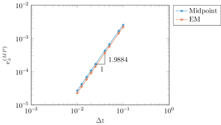
Figure 11: Accuracy study: Relative error in the position w.r.t midpoint rule

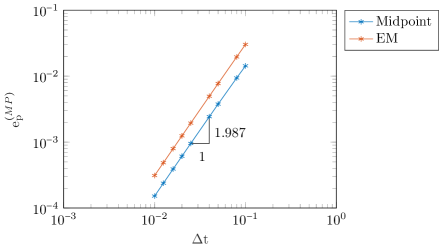
Figure 12: Accuracy study: Relative error in the linear momentum w.r.t midpoint rule

5.5 Energy consistency study

We consider now 64 atoms inside a three-dimensional box $[-L/2,L/2]^{3}$, initially arranged in a perfect diamond cubic lattice structure. This lattice will be disrupted during the simulation as we consider an initial velocity associated to each atom such that the total initial kinetic energy is approximately $768.22$.

Table 4: Energy consistency study: Data used in the simulation

Material parameters	$\epsilon$	1	Initial configuration
	$A$	7.049556277
	$B$	0.6022245584
	$\sigma$	1
	$\lambda$	210
	$p$	4
	$q$	0
	$a$	2
	$\gamma$	1.2
Mass	$m^{a}$	1
Sidelength	$L$	4
Newton tolerance	-	10-9
Simulation duration	$T$	16
Time step size	$\Delta t$	0.04

For the chosen time step size, the midpoint rule clearly violates the conservation of the total energy, see Figure 13, leading to an energy blow-up and finally to a termination of the simulation, indicated by the black line on the same figure.

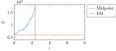
Figure 13: Energy consistency study: Total energy

The largest contribution to the algorithmic energy error is due to the midpoint approximation of the forces generated from the three-body contribution of the Stillinger-Weber potential. It can be observed in Figure 14 that the potential energy of the two-body terms remains bounded, while the potential energy of the three-body terms increases unphysically causing the energy blow-up and, ultimately, the termination of the simulation.

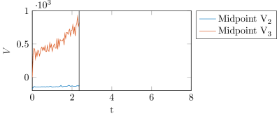
Figure 14: Energy consistency study: Potential energies using the Midpoint rule

In contrast, using the EM method both contributions to the potential energy of the system remain bounded. See Figure 15.

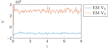
Figure 15: Energy consistency study: Potential energies using the EM method

As expected, the EM method preserves the total energy up to round-off errors. See Figure 16.

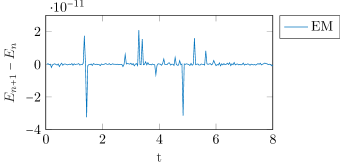
Figure 16: Energy consistency study: Total energy difference

Eventually, as illustrated in Figure 17, the evolution of the kinetic energy reveals that the EM solution reaches thermodynamic equilibrium for the chosen time step size, in contrast with the midpoint rule.

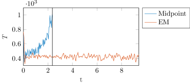
Figure 17: Energy consistency study: Kinetic energy

6 Energy-Momentum methods for periodic systems described by the embedded-atom method

In addition to three-body potentials of the type described in Section 5, more elaborate and accurate potentials include multi-body effects through an environment-dependent variable, resulting in effective potential that are extremely common, for example, in the simulation of metals. One of the most popular interatomic potentials of this class is the one employed in the embedded-atom method (EAM) [23, 25, 26], whose use in the context of conserving schemes is analyzed in this section. The interatomic potential in this case is of the form

$$V=\frac{1}{2}\sum_{\begin{subarray}{c}a,b=1\\ b\neq a\end{subarray}}^{N}\tilde{V}\left(d_{T}({\boldsymbol{x}}^{a},{\boldsymbol{x}}^{b})\right)+\sum_{a=1}^{N}\tilde{F}\left(\bar{\rho}^{a}\right)\ .$$ (73)

The EAM potential consists of a pair potential contribution and electronic energies $\tilde{F}(\bar{\rho}^{a})$. The latter is due to the embedding of $a$-th atom in a homogeneous electron gas of density $\bar{\rho}^{a}$ [27]. The background electron density function $\bar{\rho}^{a}$ is a linear superposition of contributions from each neighbor atom such that the electronic energy $\tilde{F}(\bar{\rho}^{a})$ of the $a$-th atom depends on the interatomic distance $d_{T}({\boldsymbol{x}}^{a},{\boldsymbol{x}}^{b})$ to each neighbor.

In the case of metals, the environment of each atom is a nearly uniform electron gas and therefore the embedded-atom approximation is reasonable. Since we already investigated pair potentials in Section 4, we now investigate the discretization of the forces due to the electronic energy, noting that the resultant forces in an EAM potential must include the forces due to the pair potential, as well.

6.1 Equation of motion

We consider a system of $N$ particles in a periodic box $\mathcal{B}$ of side $L$ with equations of motion (11) and an effective potential that depends only on the electronic energy of each particle, that is

$$V=\sum_{a=1}^{N}\tilde{F}\left(\sum_{\begin{subarray}{c}b=1\\ b\neq a\end{subarray}}^{N}g_{b}\left(d_{T}({\boldsymbol{x}}^{a},{\boldsymbol{x}}^{b})\right)\right),$$ (74)

where $\tilde{V}:\mathbb{R}^{+}\cup\{0\}\to\mathbb{R}$. Here, $g_{a}:\mathbb{R}^{+}\cup\{0\}\to\mathbb{R}$ is a function of the relative interatomic distance which represents a spherical electron density field around the isolated $a$-th particle [27]. Using the definitions in eq. 21, the background energy density is then given by

$$\bar{\rho}^{a}=\sum_{\begin{subarray}{c}b=1\\ b\neq a\end{subarray}}^{N}g_{b}\left(\bar{r}^{ab}\right)\ .$$ (75)

The forces acting on the particles are defined by eq. 12 and have the standard form

$$\boldsymbol{f}^{a}=\sum_{\begin{subarray}{c}b=1\\ a\neq b\end{subarray}}^{N}\boldsymbol{f}^{ab}\ ,\qquad\mathrm{with}\qquad\boldsymbol{f}^{ab}:=\varphi^{ab}\frac{\bar{\boldsymbol{r}}^{ab}}{\bar{r}^{ab}}\ ,$$ (76)

where the strength of the force has now the structure

$$\varphi^{ab}=\tilde{F}^{\prime}\left(\bar{\rho}^{a}\right)g_{b}^{\prime}\left(\bar{r}^{ab}\right)+\tilde{F}^{\prime}(\bar{\rho}^{b})g_{a}^{\prime}\left(\bar{r}^{ab}\right)\ .$$ (77)

We observe that, for this potential contribution, the direction of the interatomic force depends only on the difference between the $a$-th and the $b$-th particle, while its strength is further determined by the background electron density at the $a$-th and $b$-th particle.

6.2 Time discretization

We consider now the integration in time of the equations of motion (11) of a system in the periodic box $\mathcal{B}$ and effective potential (73) and employ the same time integration strategy as outlined in Section 4.2.

6.2.1 Midpoint scheme

The canonical midpoint rule approximates the equation of motion by the implicit formula (24), where the midpoint approximation of the force acting on the $a$-th particle in the direction of the $b$-th particle is given by

$$\boldsymbol{f}_{MP}^{ab} =\varphi^{ab}_{MP}\frac{\bar{\boldsymbol{r}}^{ab}_{n+1/2}}{{|\bar{\boldsymbol{r}}^{ab}_{n+1/2}|}},$$ (78)

$$\varphi^{ab}_{MP} =\tilde{F}^{\prime}\left(\bar{\rho}^{a}_{MP}\right)g_{b}^{\prime}\left({\bar{{r}}^{ab}_{n+1/2}}\right)+\tilde{F}^{\prime}(\bar{\rho}^{b}_{MP})g_{a}^{\prime}\left({\bar{{r}}^{ab}_{n+1/2}}\right),$$

and the midpoint approximation of the background energy density reads

$$\bar{\rho}_{MP}^{a}=\sum_{\begin{subarray}{c}b=1\\ b\neq a\end{subarray}}^{N}g_{b}\left(\bar{{r}}^{ab}_{n+1/2}\right)\ .$$ (79)

As in the continuous case, the weak law of action and reaction is satisfied and responsible for the conservation of total linear momentum of the system, see Section 4.2.1.

6.2.2 Energy and momentum conserving discretization

As illustrated in previous sections, it is possible to construct a perturbation of the midpoint rule which, in addition to preserving the total linear momentum, preserves the total energy. For that, we follow once more the steps presented in Section 4.2.2. The partitioned discrete gradient will be again with a slightly different structure due to the nature of the embedded function. The partitioned discrete gradient assumes the form

$$\mathsf{D}_{\boldsymbol{x}^{a}}V=-\sum_{\begin{subarray}{c}a,b=1\\ a\neq b\end{subarray}}^{N}\boldsymbol{f}^{ab}_{algo}=-\sum_{\begin{subarray}{c}a,b=1\\ a\neq b\end{subarray}}^{N}\frac{1}{2}\left(\boldsymbol{f}^{ab}_{n,n+1}+\boldsymbol{f}^{ab}_{n+1,n}\right),$$ (80)

with the contributions

$$\boldsymbol{f}^{ab}_{n,n+1} =\boldsymbol{f}_{MP}^{ab}+\frac{\Delta\tilde{F}^{ab}_{n,n+1}-\boldsymbol{f}_{MP}^{ab}\cdot(\boldsymbol{r}^{ab}_{n+1}-\boldsymbol{r}^{ab}_{n})}{|\boldsymbol{r}^{ab}_{n+1}-\boldsymbol{r}^{ab}_{n}|}\;\boldsymbol{n}\ ,$$ (81)

$$\boldsymbol{f}^{ab}_{n+1,n} =\boldsymbol{f}_{MP}^{ab}+\frac{\Delta\tilde{F}^{ab}_{n+1,n}-\boldsymbol{f}_{MP}^{ab}\cdot(\boldsymbol{r}^{ab}_{n+1}-\boldsymbol{r}^{ab}_{n})}{|\boldsymbol{r}^{ab}_{n+1}-\boldsymbol{r}^{ab}_{n}|}\;\boldsymbol{n}\ ,$$

for which we introduced the compact notation

$$\Delta\tilde{F}^{ab}_{n,n+1} =\tilde{F}(\bar{\rho}^{a}_{n,n+1}(\bar{r}^{ab}_{n+1}))-\tilde{F}(\bar{\rho}^{a}_{n,n+1}(\bar{r}^{ab}_{n}))$$ (82)

$$+\tilde{F}(\bar{\rho}^{b}_{n,n+1}(\bar{r}^{ab}_{n+1}))-\tilde{F}(\bar{\rho}^{b}_{n,n+1}(\bar{r}^{ab}_{n}))\ ,$$

$$\Delta\tilde{F}^{ab}_{n+1,n} =\tilde{F}(\bar{\rho}^{a}_{n+1,n}(\bar{r}^{ab}_{n+1}))-\tilde{F}(\bar{\rho}^{a}_{n+1,n}(\bar{r}^{ab}_{n}))$$

$$+\tilde{F}(\bar{\rho}^{b}_{n+1,n}(\bar{r}^{ab}_{n+1}))-\tilde{F}(\bar{\rho}^{b}_{n+1,n}(\bar{r}^{ab}_{n}))\ ,$$

and

$$\bar{\rho}^{a}_{n,n+1}(\bar{r}^{ab}) =\sum_{d=1}^{b-1}g_{a}(\bar{r}^{ad}_{n})+g_{a}(\bar{r}^{ab})+\sum_{e=b+1}^{N}g_{a}(\bar{r}^{ae}_{n+1})\ ,$$ (83)

$$\bar{\rho}^{a}_{n+1,n}(\bar{r}^{ab}) =\sum_{d=1}^{b-1}g_{a}(\bar{r}^{ad}_{n+1})+g_{a}(\bar{r}^{ab})+\sum_{e=b+1}^{N}g_{a}(\bar{r}^{ae}_{n})\ .$$

The densities $\bar{\rho}^{b}_{n,n+1}(\bar{r}^{ab})$ and $\bar{\rho}^{b}_{n+1,n}(\bar{r}^{ab})$ are defined similarly.

To show that the integrator exactly preserves the total momentum, it suffices to follow the proof in Section 4.2.2. The critical condition that a conserving scheme must satisfy reads now:

$$\sum^{N}_{\begin{subarray}{c}b=1\\ a<b\end{subarray}}\boldsymbol{f}_{algo}^{ab}\cdot(\boldsymbol{r}^{ab}_{n+1}-\boldsymbol{r}^{ab}_{n})=\sum_{a=1}^{N}\left(\tilde{F}(\bar{\rho}^{a}_{n+1})-\tilde{F}(\bar{\rho}^{a}_{n})\right)\ ,$$ (84)

which is indeed satisfied by the proposed method.

6.3 Interatomic potential

We consider for our subsequent analysis the Lennard-Jones-Baskes (LJB) EAM model [25, 36], which is the extension of the Lennard-Jones material model into the many-body regime of the EAM formalism [37]. The total potential energy of the LJB model is given by

$$\tilde{V}=\frac{1}{2}\sum_{\begin{subarray}{c}a,b=1\\ a\neq b\end{subarray}}^{N}V(\bar{r}^{ab})+\sum_{\begin{subarray}{c}a=1\end{subarray}}^{N}\tilde{F}(\bar{\rho}^{a})\ .$$ (85)

The two body part has been introduced in Section 4.3. For the EAM contribution we further define

$$\tilde{F}(\bar{\rho}^{a}) =\frac{1}{2}\epsilon AZ_{1}\bar{\rho}^{a}\left(\textrm{ln}\left(\bar{\rho}^{a}\right)-1\right),$$ (86)

$$\bar{\rho}^{a} =\frac{1}{Z_{1}}\sum_{\begin{subarray}{c}b=1\\ b\neq a\end{subarray}}^{N}g_{b}\left({|\bar{\boldsymbol{r}}^{ab}|}\right),$$

$$g_{b}\left({|\bar{\boldsymbol{r}}^{ab}|}\right) =\begin{cases}\exp\left(-\beta\left(\sigma^{-1}|\bar{\boldsymbol{r}}^{ab}|-1\right)\right)&\text{if}\ |\bar{\boldsymbol{r}}^{ab}|<r_{c}\\ 0&\text{otherwise}\ ,\end{cases}$$

where $\epsilon$, $\sigma$, $\beta$, $A$, $r_{c}$ and $Z_{1}$ are material parameters.

6.4 Numerical evaluation

Since we already investigated pair potentials in Section 4, we focus on the EAM part of the LJB material model for the following numerical evaluations.

6.4.1 Accuracy study

A three-dimensional box $[-L/2,L/2]^{3}$ is now considered with 5 particles inside it. The particles form a unit body-centered cubic (BCC) cell of side $2$, centered within the box. Starting from rest, the system builds up kinetic energy due to the fact that the particles in the exterior of the BCC crystal are not in equilibrium. Further parameters of the simulation can be found in Table 5.

Table 5: Accuracy study: Data used in the simulation

Material parameters	$\epsilon$	2	Initial configuration
	$A$	1
	$\sigma$	1
	$\beta$	4
	$Z_{1}$	12
	$r_{c}$	3
Mass	$m^{a}$	1
Side length	$L$	6
Newton tolerance	-	10-6
Simulation duration	$T$	0.5
Reference time step size	$\Delta t_{\text{ref}}$	0.0001
Time step size	$\Delta t$	0.0005, 0.001,
		0.002, 0.0025,
		0.004, 0.005,
		0.01, 0.02,
		0.025

Proceeding as in Section 4.4.1, we perform an accuracy analysis of the EM integrator using the midpoint rule as the reference solution. To study the convergence of the numerical solutions, we employ ten time steps of decreasing size and the error measures defined in (51). Figures 18 and 19 confirm again that both the midpoint rule and the EM method are second order accurate approximations.

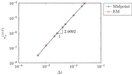
Figure 18: Accuracy study: Relative error in the position w.r.t midpoint rule

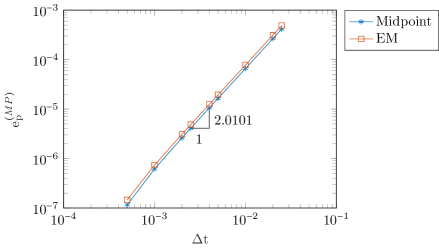
Figure 19: Accuracy study: Relative error in the momentum w.r.t midpoint rule

6.5 Energy consistency study

We consider in this last example 108 atoms inside a three-dimensional box $[-L/2,L/2]^{3}$, where the atoms are arranged in a perfect face-centered cubic (FCC) lattice structure. This FCC lattice is perturbed by the initial velocities of the atoms which are imparted in such a way that the total initial kinetic energy is approximately $3.251$. Further parameters of the simulation can be found in Table 6.

Table 6: Energy consistency study: Data used in the simulation

Material parameters	$\epsilon$	2	Initial configuration
	$A$	1
	$\sigma$	1
	$\beta$	4
	$Z_{1}$	12
	$r_{c}$	3
Mass	$m^{a}$	1
Side length	$L$	6
Newton tolerance	-	10-8
Simulation duration	$T$	40
Time step size	$\Delta t$	0.1

For the time step selected, the midpoint rule clearly violates the conservation of total energy (see Figure 20). As in previous examples, this leads to an energy blow-up and finally to a termination of the simulation, indicated by the black line on the same figure.

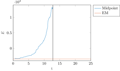
Figure 20: Energy consistency study: Total energy

In contrast, the EM method preserves the total energy up to round off errors, see Figure 21.

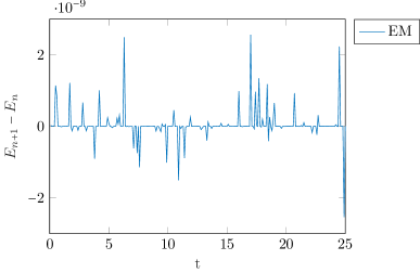
Figure 21: Energy consistency study: Total energy difference

Finally, and as in the previous examples, Figure 22 shows that the EM, but not the midpoint rule, is able to evolve the system of particles up to thermodynamic equilibrium.

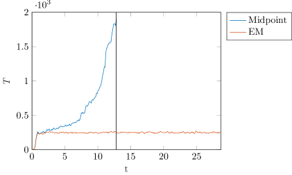
Figure 22: Energy consistency study: Kinetic energy

7 Summary of main results

Conserving schemes have been employed during more than four decades for the accurate and robust approximation of Hamiltonian problems in mechanics. However, in the field of molecular dynamics, where time integrators are routinely employed and are key to their usefulness, the use of conserving schemes has barely been explored.

In this work we have analyzed energy and momentum conserving schemes in the context of molecular dynamics. This second order, implicit methods are an interesting alternative to other commonly used integrators and we have proven than, in addition to exhibiting exact energy conservation, are more robust than the midpoint rule, the canonical second order implicit method.

The article has focused on the design of Energy-Momentum schemes for molecular dynamics in the view of three issues that are characteristic and unique to these problems. First, the numerical treatment of dynamics in periodic domains; second, the discretization of three-body potentials; last, the study of interatomic functional potentials. Neither of these three topics had been previously studied in the context of conserving schemes, to the authors’ knowledge. However, the three of them are key for their implementation and clearly have an impact on their performance.

Some of the most practical results of this work are new expressions for Energy-Momentum approximations in fairly general problems in molecular dynamics. These approximations account for the three key issues mentioned before, and can be shown to preserve linear momentum and energy, exactly, while exhibiting a remarkable robustness.

8 Acknowledgements

Support for M.S. was provided by the Deutsche Forschungsgemeinschaft (DFG) under Grant BE 2285/13-1 and the Research Travel Grant of the Karlsruhe House of Young Scientists (KYHS). This support is gratefully acknowledged.

References

- [1] E. Hairer, C. Lubich, G. Wanner, Geometric numerical integration: structure-preserving algorithms for ordinary differential equations, Vol. 31, Springer Science & Business Media, 2006.
- [2] B. Leimkuhler, S. Reich, Simulating Hamiltonian Dynamics, Vol. 14, Cambridge University Press, 2004.
- [3] R. A. LaBudde, D. Greenspan, Energy and momentum conserving methods of arbitrary order for the numerical integration of equations of motion, Numer. Math. 26 (1) (1976) 1–16.
- [4] R. A. LaBudde, D. Greenspan, Energy and momentum conserving methods of arbitrary order for the numerical integration of equations of motion, Numer. Math. 25 (4) (1975) 323–346.
- [5] J. Simo, N. Tarnow, The discrete energy-momentum method. conserving algorithms for nonlinear elastodynamics, ZAMM - Z. Angew. Math. Mech. 43 (5) (1992) 757–792.
- [6] O. Gonzalez, Exact energy-momentum conserving algorithms for general models in nonlinear elasticity, Comput. Methods Appl. Mech. Engrg. 190 (2000) 1763–1783.
- [7] J. C. Simo, N. Tarnow, A new energy and momentum conserving algorithm for the non-linear dynamics of shells, Int. J. Numer. Meth. Engng. 37 (15) (1994) 2527–2549.
- [8] J. C. Simo, N. Tarnow, M. Doblaré, Non-linear dynamics of three-dimensional rods: exact energy and momentum conserving algorithms, Int. J. Numer. Meth. Engng. 38 (9) (1995) 1431–1473.
- [9] H. G. Zhong, M. A. Crisfield, An energy-conserving co-rotational procedure for the dynamics of shell structures, Eng. Computation 15 (5) (1998) 552–576.
- [10] I. Romero, F. Armero, An objective finite element approximation of the kinematics of geometrically exact rods and its use in the formulation of an energy-momentum conserving scheme in dynamics, Int. J. Numer. Meth. Engng. 54 (12) (2002) 1683–1716.
- [11] J. C. García Orden, J. M. Goicolea, Conserving properties in constrained dynamics of flexible multibody systems, Multibody Syst. Dyn. 4 (2000) 225–244.
- [12] P. Betsch, S. Uhlar, Energy-momentum conserving integration of multibody dynamics, Multibody Syst. Dyn. 17 (2007) 243–249.
- [13] R. I. McLachlan, G. R. W. Quispel, N. Robidoux, Geometric integration using discrete gradients, Philos. Trans. Roy. Soc. London Ser. A 357 (1999) 1021–1045.
- [14] E. Celledoni, V. Grimm, R. I. McLachlan, D. I. McLaren, D. O’Neale, B. Owren, G. R. W. Quispel, Preserving energy resp. dissipation in numerical PDEs using the “Average Vector Field” method, J. Comput. Phys. 231 (20) (2012) 6770–6789.
- [15] S. Toxvaerd, Energy conservation in molecular dynamics, J. Comput. Phys. 52 (1) (1983) 214–216.
- [16] D. C. Rapaport, The art of molecular dynamics simulation, Cambridge University Press, 2004.
- [17] R. D. Skeel, D. J. Hardy, J. C. Phillips, Correcting mesh-based force calculations to conserve both energy and momentum in molecular dynamics simulations, J. Comput. Phys. 225 (1) (2007) 1–5.
- [18] M. P. Allen, D. J. Tildesley, Computer simulation of liquids, Clarendon Press, 1989.
- [19] C. Saluena, J. B. Avalos, Molecular dynamics algorithm enforcing energy conservation for microcanonical simulations, Phys. Rev. E 89 (5) (2014) 053314.
- [20] M. Griebel, G. Zumbusch, S. Knapek, Numerical simulation in molecular dynamics. Numerics, algorithms, parallelization, Texts in Computational Science and Engineering, Springer, Berlin, 2007.
- [21] B. R. Brooks, R. E. Bruccoleri, B. D. Olafson, D. J. States, S. a. Swaminathan, M. Karplus, Charmm: a program for macromolecular energy, minimization, and dynamics calculations, J. Comput. Chem. 4 (2) (1983) 187–217.
- [22] F. H. Stillinger, T. A. Weber, Computer simulation of local order in condensed phases of silicon, Phys. Rev. B 31 (8) (1985) 5262.
- [23] M. S. Daw, M. I. Baskes, Embedded-atom method: Derivation and application to impurities, surfaces, and other defects in metals, Phys. Rev. B 29 (12) (1984) 6443.
- [24] M. S. Daw, Model of metallic cohesion: The embedded-atom method, Phys. Rev. B 39 (11) (1989) 7441.
- [25] M. I. Baskes, Modified embedded-atom potentials for cubic materials and impurities, Phys. Rev. B 46 (5) (1992) 2727.
- [26] M. S. Daw, S. M. Foiles, M. I. Baskes, The embedded-atom method: a review of theory and applications, Materials Science Reports 9 (7-8) (1993) 251–310.
- [27] E. B. Tadmor, R. E. Miller, Modeling materials: continuum, atomistic and multiscale techniques, Cambridge University Press, 2011.
- [28] J. E. Lennard-Jones, On the determination of molecular fields. ii. from the equation of state of gas, Proc. Roy. Soc. A 106 (1924) 463–477.
- [29] H. Goldstein, C. Poole, J. Safko, Classical mechanics (2002).
- [30] V. A. Kuzkin, On angular momentum balance for particle systems with periodic boundary conditions, ZAMM - Z. Angew. Math. Mech. 95 (11) (2015) 1290–1295.
- [31] J. Haile, I. Johnston, A. J. Mallinckrodt, S. McKay, Molecular dynamics simulation: elementary methods, Comput. Phys. 7 (6) (1993) 625–625.
- [32] O. Gonzalez, Design and analysis of conserving integrators for nonlinear hamiltonian systems with symmetry, Ph.D. thesis, Stanford University Stanford, CA (1996).
- [33] I. Romero, An analysis of the stress formula for energy-momentum methods in nonlinear elastodynamics, Comput. Mech. 50 (5) (2012) 603–610.
- [34] S. Plimpton, Fast parallel algorithms for short-range molecular dynamics, Tech. rep., Sandia National Labs., Albuquerque, NM (United States) (1993).
- [35] D. L. Kreher, D. R. Stinson, Combinatorial Algorithms, Generation, Enumeration, and Search, CRC Press, Boca Raton, FL, 1999.
- [36] M. Baskes, Many-body effects in fcc metals: a lennard-jones embedded-atom potential, Phys. Rev. Lett. 83 (13) (1999) 2592.
- [37] S. Srinivasan, M. Baskes, On the lennard–jones eam potential, P. Roy. Soc. Lond. A Mat. 460 (2046) (2004) 1649–1672.