Solving nonlinear systems of equations via spectral residual methods: stepsize selection and applications

Abstract

Spectral residual methods are derivative-free and low-cost per iteration procedures for solving nonlinear systems of equations. They are generally coupled with a nonmonotone linesearch strategy and compare well with Newton-based methods for large nonlinear systems and sequences of nonlinear systems. The residual vector is used as the search direction and choosing the steplength has a crucial impact on the performance. In this work we address both theoretically and experimentally the steplength selection and provide results on a real application such as a rolling contact problem.

Keywords. Nonlinear systems of equations, spectral gradient methods, steplength selection, approximate norm descent methods

1 Introduction

This work addresses the solution of the nonlinear system of equations

$$F(x)=0,$$ (1)

with $F:\mathbb{R}^{n}\rightarrow\mathbb{R}^{n}$ continuously differentiable, by means of spectral residual methods. Spectral residual methods were introduced in [25] and starting from the proposal in [26] consist of iterative procedures for solving (1) without the use of derivative information. Given the iterate $x_{k}$, these methods use the residual vectors $\pm F(x_{k})$ in a systematic way and select the step $x_{k+1}-x_{k}$ along either the direction $(-\beta_{k}F(x_{k}))$ or $(\beta_{k}F(x_{k}))$ with $\beta_{k}$ being a nonzero steplength inspired by the Barzilai and Borwein method for the unconstrained minimization problem $\min_{x\in\mathbb{R}^{n}}f(x)$. Similarly to the Barzilai and Borwein method for unconstrained optimization, $\|F\|$ does not decrease monotonically along iterations and its effectiveness heavily relies on the steplength $\beta_{k}$ used.

Spectral residual methods have received a large attention since they are low-cost per iteration and require a low memory storage being matrix free, see e.g. [21, 27, 25, 26, 34, 31, 35, 41]. They belong to the class of Quasi-Newton methods which are particularly attractive when the Jacobian matrix of $F$ is not available analytically or its computation is not relatively easy. Quasi-Newton methods showed to be effective both in the solution of large nonlinear systems and in the solution of sequences of medium-size nonlinear systems as those arising in applications where sequences are generated by model refinement procedures, see e.g., [26, 21, 31, 25, 5, 41].

It is well known that the performance of the Barzilai and Borwein method does not depend on the decrease of the objective function at each iteration but relies on the relationship between the steplengths used and the eigenvalues of the average Hessian matrix of $f$ [3, 15, 36]. Based on such feature, several strategies for steplength selection have been proposed to enhance the performance of the method, see e.g., [8, 9, 15, 10, 12, 16]. On the other hand, to our knowledge, an analogous study of the relationship between the steplengths originated by spectral methods and the eigenvalues of the average Jacobian matrix of $F$ has not been carried out, and the impact of the choice of the steplenghts on the convergence history has not been investigated in details. The aim of this paper is to analyze the properties of the spectral residual steplengths and study how they affect the performance of the methods. This aim is addressed both from a theoretical and experimental point of view.

The main contributions of this work are: the theoretical analysis of the steplengths proposed in the literature and of their impact on the norm of $F$ also with respect to the nonmonotone behaviour imposed by globalization strategies; the analysis of the performance of spectral methods with various rule for updating the steplengths. Rules based on adaptive strategies that suitably combine small and large steplengths result by far more effective than rules based on static choices of $\beta_{k}$ and, inspired by the steplength rules proposed in the literature for unconstrained minimization problems, we propose and extensively test adaptive steplength strategies. Numerical experience is conducted on sequences of nonlinear systems arising from rolling contact models which play a central role in many important applications, such as rolling bearings and wheel-rail interaction [23, 24]. Solving these models gives rise to sequences which consist of a large number of medium-size nonlinear systems and represent a relevant benchmark test set for the purpose of this work.

The paper is organized as follows. Section 2 introduces spectral residual methods. In Section 3 and 4 we provide a theoretical analysis of the steplengths including their impact on the behaviour of $\|F_{k}\|$ and on a standard nonmonotone linesearch. In Section 5 we introduce the spectral residual method used in our tests and provide a theoretical investigation. The experimental part is developed in Section 6 where we describe several strategies for selecting the steplength, introduce our test set and discuss the numerical results obtained. Some conclusions are presented in Section 7.

1.1 Notations

The symbol $\|\cdot\|$ denotes the Euclidean norm, $I$ denotes the identity matrix, $J$ denotes the Jacobian matrix of $F$. Given a symmetric matrix $M$, $\{\lambda_{i}(M)\}_{i=1}^{n}$ denotes the set of eigenvalues of $M$, $\lambda_{\min}(M)$ and $\lambda_{\max}(M)$ denote the minimum and maximum eigenvalue of $M$ respectively, and $\{v_{i}\}_{i=1}^{n}$ denotes a set of associated orthonormal eigenvectors. Given a sequence of vectors $\{x_{k}\}$, for any function $f$ we let $f_{k}=f(x_{k})$.

2 Preliminaries

In the seminal paper [2] Barzilai and Borwein proposed a gradient method for the unconstrained minimization

$$\min_{x\in\mathbb{R}^{n}}f(x),$$ (2)

where $f:\mathbb{R}^{n}\rightarrow\mathbb{R}$ is a given differentiable function. Given an initial guess $x_{0}\in\mathbb{R}^{n}$, the Barzilai-Borwein (BB) iteration is defined by

$$x_{k+1}=x_{k}-\alpha_{k}\nabla f_{k},$$ (3)

where $\alpha_{k}$ is a positive steplength inspired by Quasi-Newton methods for unconstrained optimization [11]. In Quasi-Newton methods, the step $p_{k}=x_{k+1}-x_{k}$ solves the linear system

$$B_{k}p_{k}=-\nabla f_{k},$$ (4)

and $B_{k}$, $k\geq 1$, satisfies the secant equation, i.e.,

$$B_{k}p_{k-1}=z_{k-1},\quad p_{k-1}=x_{k}-x_{k-1},\quad z_{k-1}=\nabla f_{k}-\nabla f_{k-1}.$$ (5)

Letting $B_{k}=\alpha^{-1}\,I$ and imposing condition (5), Barzilai and Borwein derived two steplengths which are the least-square solutions of the following problems:

$$\alpha_{k,1} =\mathop{\rm argmin}_{\alpha}\|\alpha^{-1}p_{k-1}-z_{k-1}\|_{2}^{2}=\frac{p_{k-1}^{T}p_{k-1}}{p_{k-1}^{T}z_{k-1}},$$ (6)

$$\alpha_{k,2} =\mathop{\rm argmin}_{\alpha}\|p_{k-1}-\alpha z_{k-1}\|_{2}^{2}=\frac{p_{k-1}^{T}z_{k-1}}{z_{k-1}^{T}z_{k-1}}.$$ (7)

The second least-squares formulation is obtained from the first by symmetry. The steplength $\alpha_{k}$ in (3) is set to be positive, bounded away from zero and not too large, i.e., $\alpha_{k}\in[\alpha_{\min},\,\alpha_{\max}]$ for some positive $\alpha_{\min}$, $\alpha_{\max}$; to this end, one of the two scalars $\alpha_{k,1},\,\alpha_{k,2}$ is used and the thresholds $\alpha_{\min}$, $\alpha_{\max}$ are applied to it, see e.g., [3, 15, 12].

Choosing $B_{k}=\alpha^{-1}\,I$ yields a low-cost iteration while the use of the steplengths $\alpha_{k,1}$, $\alpha_{k,2}$ yields a considerable improvement in the performance with respect to the classical steepest descent method [2, 15]. The BB method is commonly employed in the solution of large unconstrained optimization problems (2) and the behaviour of the sequence $\{f(x_{k})\}$ is typically nonmonotone, possibly severely nonmonotone, in both the cases of quadratic and general nonlinear functions $f$ [15, 17, 38]. The performance of the BB method depends on the relationship between the steplength $\alpha_{k}$ and the eigenvalues of the average Hessian matrix $\int_{0}^{1}\nabla^{2}f(x_{k-1}+t\,p_{k-1})\,dt$; hence this approach is also denoted as spectral method and an extensive investigation on steplength’s selection has been carried on [8, 9, 15, 10, 12, 16].

The extension of this approach to the solution of nonlinear systems of equations (1) was firstly proposed by La Cruz and Raydan in [25]. Here we summarize such a proposal and the issues that were inherited by subsequent procedures falling into such framework and designed for both general nonlinear systems [21, 27, 25, 26, 34, 31, 41] and for monotone nonlinear systems [44, 40, 1, 32, 29, 30]. Instead of applying the spectral method to the merit function

$$f(x)=\|F(x)\|^{2},$$ (8)

the BB approach is specialized to the Newton equation yielding the so-called spectral residual method. Thus, let $p_{-}$ satisfy the linear system

$$B_{k}p_{-}=-F_{k},$$ (9)

and let $B_{k}=\beta^{-1}I$ satisfy the secant equation

$$B_{k}p_{k-1}=y_{k-1},\quad p_{k-1}=x_{k}-x_{k-1},\quad y_{k-1}=F_{k}-F_{k-1}.$$

Reasoning as in BB method, two steplengths are derived:

$$\beta_{k,1} = \frac{p_{k-1}^{T}p_{k-1}}{p_{k-1}^{T}y_{k-1}},$$ (10)

$$\beta_{k,2} = \frac{p_{k-1}^{T}y_{k-1}}{y_{k-1}^{T}y_{k-1}}.$$ (11)

These scalars may be positive, negative or even null; moreover $\beta_{k,1}$ is not well defined if $p_{k-1}^{T}y_{k-1}=0$ and $\beta_{k,2}$ is not well defined if $y_{k-1}=0$. In practice, the steplength $\beta_{k}$ is chosen equal either to $\beta_{k,1}$ or to $\beta_{k,2}$ as long as it results to be bounded away from zero and $|\beta_{k}|$ is not too large, i.e., $|\beta_{k}|\in[\beta_{\min},\,\beta_{\max}]$ for some positive $\beta_{\min}$, $\beta_{\max}$. The step resulting from (9) turns to be of the form $p_{-}=-\beta_{k}F_{k}.$ But, once $\beta_{k}$ is fixed, the $k$th iteration of the spectral residual method employs the residual directions $\pm F_{k}$ in a systematic way and tests both the steps

$$p_{-}=-\beta_{k}F_{k}\quad\mbox{and}\quad p_{+}=+\beta_{k}F_{k},$$

for acceptance using a suitable linesearch strategy. The use of both directions $\pm F_{k}$ is motivated by the fact that, contrary to $(-\alpha_{k}\nabla f_{k})$, $\alpha_{k}>0$, in (3), $(-\beta_{k}F_{k})$ is not necessarily a descent direction for (8) at $x_{k}$; the value $\nabla f_{k}^{T}(-\beta_{k}F_{k})=-2\beta_{k}F_{k}^{T}J_{k}F_{k}$ could be positive, negative or null. On the other hand, if $F_{k}^{T}J_{k}F_{k}\neq 0$, trivially either $(-\beta_{k}F_{k})$ or $\beta_{k}F_{k}$ is a descent direction for $f$.

Analogously to the spectral method, the spectral residual method is characterized by a nonmonotone behaviour of $\{\|F_{k}\|\}$ and is implemented using nonmonotone line search strategies. The adaptation of the spectral method to nonlinear systems is low-cost per iteration since the computation of $\beta_{k,1}$ and $\beta_{k,2}$ is inexpensive and the memory storage is low, and turned out to be effective in the solution of medium and large nonlinear systems, see e.g., [21, 27, 25, 26, 34, 41].

Unlike the context of BB method for unconstrained optimization, to our knowledge a systematic analysis of the stepsizes $\beta_{k,1}$ and $\beta_{k,2}$ in the context of the solution of nonlinear systems and their impact on convergence history has not been carried out. The steplength $\beta_{k,1}$ has been used in most of the works on this subject [27, 25, 26, 34, 31]. On the other hand, in [21] it was observed experimentally that alternating $\beta_{k,1}$ and $\beta_{k,2}$ along iterations was beneficial for the performance and in [41] it was observed experimentally that using $\beta_{k,2}$ performed better in terms of robustness with respect to using $\beta_{k,1}$.

In the next two sections we will analyze the two steplengths $\beta_{k,1}$ and $\beta_{k,2}$ and provide: their expression in terms of the spectrum of average matrices associated to the Jacobian matrix of $F$; their mutual relationship; their impact on the behaviour of $\|F_{k}\|$ and on a standard nonmonotone linesearch.

The matrices involved in our analysis are the following. Given a square matrix $A$, we let $A_{S}=\frac{1}{2}(A+A^{T})$ be the symmetric part of $A$, $G_{k-1}$ be the average matrix associated to the Jacobian $J$ of $F$ around $x_{k-1}$

$$G_{k-1}\stackrel{{\scriptstyle\rm def}}{{=}}\int_{0}^{1}J(x_{k-1}+t\,p_{k-1})\,dt,$$ (12)

and $(G_{S})_{k-1}$ be the average matrix associated to the symmetric part $J_{S}$ of $J$ around $x_{k-1}$

$$(G_{S})_{k-1}\stackrel{{\scriptstyle\rm def}}{{=}}\int_{0}^{1}J_{S}(x_{k-1}+t\,p_{k-1})\,dt.$$ (13)

Moreover, given a symmetric matrix $M$ and a nonzero vector $p$, we employ the Rayleigh quotient defined as

$$q(M,p)=\frac{p^{T}Mp}{p^{T}p},$$ (14)

and the following property [18, Theorem 8.1-2]

$$\lambda_{\min}(M)\leq q(M,p)\leq\lambda_{\max}(M).$$ (15)

3 Analysis of the steplengths $\beta_{k,1}$ and $\beta_{k,2}$

We analyze the stepsizes $\beta_{k,1}$ and $\beta_{k,2}$ given in (10) and (11) making the following assumptions.

Assumption 1.

The scalars $\beta_{k,1}$ and $\beta_{k,2}$ are well defined and nonzero.

Assumption 2.

Given $x$ and $p$, $F$ is continuously differentiable in an open convex set $D\subset\mathbb{R}^{n}$ containing $x+tp$ with $t\in[0,1]$.

We note that Assumption 1 holds whenever $p_{k-1}^{T}y_{k-1}\neq 0$.

In the following lemma we analyze the mutual relationship between the stepsizes $\beta_{k,1}$ and $\beta_{k,2}$ and give their characterization in terms of suitable Rayleigh quotients for the average matrices in (12) and (13). We use repeatedly the property

$$p^{T}Ap=p^{T}A_{S}p,$$ (16)

which holds for any square matrices $A,$ $A_{S}=\frac{1}{2}(A+A^{T})$, and any vector $p$ of suitable dimension.

Lemma 3.

Let Assumption 1 hold and Assumption 2 hold with $x=x_{k-1}$, $p=p_{k-1}=\pm\beta_{k-1}F_{k-1}$. The steplengths $\beta_{k,1}$, $\beta_{k,2}$ are such that:

P1) they have the same sign and $|\beta_{k,2}|\leq|\beta_{k,1}|$;

P2) either it holds $\beta_{k,1}\leq\beta_{k,2}<0$ or $0<\beta_{k,2}\leq\beta_{k,1}$;

P3) they take the form

$$\beta_{k,1}=\frac{1}{\displaystyle q\big{(}(G_{S})_{k-1},p_{k-1}\big{)}}{\color[rgb]{0,0,0}=\frac{1}{\displaystyle q\big{(}(G_{S})_{k-1},F_{k-1}\big{)}}},$$ (17)

and

$$\beta_{k,2}=\frac{\displaystyle q\big{(}(G_{S})_{k-1},p_{k-1}\big{)}}{\displaystyle q(G_{k-1}^{T}G_{k-1},p_{k-1})}{\color[rgb]{0,0,0}=\frac{\displaystyle q\big{(}(G_{S})_{k-1},F_{k-1}\big{)}}{\displaystyle q(G_{k-1}^{T}G_{k-1},F_{k-1})}},$$ (18)

with $q(\cdot,\cdot)$ being the Rayleigh quotient in (14), $G_{k-1}$ and $(G_{S})_{k-1}$ being the matrices in (12) and (13), respectively.

Proof.   By (10) and (11), we can write

$$\beta_{k,2} = \frac{p_{k-1}^{T}p_{k-1}}{p_{k-1}^{T}y_{k-1}}\frac{(p_{k-1}^{T}y_{k-1})^{2}}{(y_{k-1}^{T}y_{k-1})(p_{k-1}^{T}p_{k-1})}$$ (19)

$$= \beta_{k,1}\frac{\|p_{k-1}\|^{2}\|y_{k-1}\|^{2}cos^{2}\varphi_{k-1}}{\|p_{k-1}\|^{2}\|y_{k-1}\|^{2}}$$

$$= \beta_{k,1}\cos^{2}\varphi_{k-1},$$

where $\varphi_{k-1}$ is the angle between $p_{k-1}$ and $y_{k-1}$, and P1) follows.

Property P2) follows as well since $\beta_{k,2}\neq 0$ by Assumption 1.

As for property P3), by the Mean Value Theorem [11, Lemma 4.1.9] and (12) we have

$$y_{k-1}=F_{k}-F_{k-1}=\int_{0}^{1}J(x_{k-1}+tp_{k-1})p_{k-1}\,dt=G_{k-1}p_{k-1}.$$

Then using (16) and (14), $\beta_{k,1}$ takes the form

$$\beta_{k,1}=\frac{p_{k-1}^{T}p_{k-1}}{p_{k-1}^{T}G_{k-1}p_{k-1}}{\color[rgb]{0,0,0}=\frac{p_{k-1}^{T}p_{k-1}}{p_{k-1}^{T}(G_{S})_{k-1}p_{k-1}}}=\frac{1}{q\big{(}(G_{S})_{k-1},p_{k-1}\big{)}},$$

while $\beta_{k,2}$ takes the form

$$\beta_{k,2}=\frac{p_{k-1}^{T}G_{k-1}p_{k-1}}{p_{k-1}^{T}(G_{k-1}^{T}G_{k-1})p_{k-1}}\frac{p_{k-1}^{T}p_{k-1}}{p_{k-1}^{T}p_{k-1}}=\frac{q\big{(}(G_{S})_{k-1},p_{k-1}\big{)}}{q(G_{k-1}^{T}G_{k-1},p_{k-1})}.$$

The rightmost equalities in (17) and (18) easily follow using the form of the step $p_{k-1}=\pm\beta_{k-1}F_{k-1}$. $\Box$

The above characterization P3) allows to derive bounds on the stepsizes $\beta_{k,1}$ and $\beta_{k,2}$ diversifying cases according to the spectral properties of the Jacobian matrix and the average matrices in (12) and (13). The relationship between $\beta_{k,1}$ and the spectral information of the symmetric part of average matrix (12) was observed in [26, 25, 34] but the following results are not contained in such references.

Lemma 4.

Let Assumption 1 hold and Assumption 2 hold with $x=x_{k-1}$, $p=p_{k-1}$. Then, the steplengths $\beta_{k,1}$ and $\beta_{k,2}$ are such that:

(i) If the Jacobian $J$ is symmetric and positive definite on the line segment in between $x_{k-1}$ and $x_{k-1}+p_{k-1}$ then $\beta_{k,1}$ and $\beta_{k,2}$ are positive and

$$\frac{1}{\lambda_{\max}(G_{k-1})}\leq\beta_{k,2}\leq\beta_{k,1}\leq\frac{1}{\lambda_{\min}(G_{k-1})};$$ (20)

(ii) if $(G_{S})_{k-1}$ in (13) is positive definite, then $\beta_{k,1}$ and $\beta_{k,2}$ are positive and

$$\max\bigg{\{}\frac{1}{\lambda_{\max}\big{(}(G_{S})_{k-1}\big{)}},\,\beta_{k,2}\bigg{\}}\leq\beta_{k,1}\leq\frac{1}{\lambda_{\min}\big{(}(G_{S})_{k-1}\big{)}},$$ (21)

$$\frac{\lambda_{\min}\big{(}(G_{S})_{k-1}\big{)}}{\lambda_{\max}(G_{k-1}^{T}G_{k-1})}\leq\beta_{k,2}\leq\min\bigg{\{}\frac{\lambda_{\max}\big{(}(G_{S})_{k-1}\big{)}}{\lambda_{\min}(G_{k-1}^{T}G_{k-1})},\beta_{k,1}\bigg{\}};$$ (22)

(iii) if $(G_{S})_{k-1}$ in (13) is indefinite and $G_{k-1}$ in (12) is nonsingular, then

(iii.1) $\beta_{k,1}$ satisfies either

$$\beta_{k,1}\leq\min\left\{\frac{1}{\lambda_{\min}\left((G_{S})_{k-1}\right)},\beta_{k,2}\right\}\ \ \>\mbox{or}\ \ \>\beta_{k,1}\geq\max\left\{\frac{1}{\lambda_{\max}\left((G_{S})_{k-1}\right)},\beta_{k,2}\right\};$$ (23)

(iii.2) $\beta_{k,2}$ satisfies either

$$0<\beta_{k,2}\leq\min\bigg{\{}\frac{\lambda_{\max}\big{(}(G_{S})_{k-1}\big{)}}{\lambda_{\min}(G_{k-1}^{T}G_{k-1})},\beta_{k,1}\bigg{\}},$$ (24)

or

$$\max\bigg{\{}\frac{\lambda_{\min}\big{(}(G_{S})_{k-1},\big{)}}{\lambda_{\max}(G_{k-1}^{T}G_{k-1})},\beta_{k,1}\bigg{\}}\leq\beta_{k,2}<0.$$ (25)

Proof.   Consider properties P1), P2) and P3) from Lemma 3.

(i) Steplengths $\beta_{k,1}$ and $\beta_{k,2}$ are positive due to (17), (18). The rightmost inequality of (20) follows from (17) and (15). The remaining part of (20) is proved observing that (18) yields

$$\beta_{k,2}=\frac{p_{k-1}^{T}G_{k-1}^{1/2}G_{k-1}^{1/2}p_{k-1}}{p_{k-1}^{T}G_{k-1}^{1/2}G_{k-1}G_{k-1}^{1/2}p_{k-1}}=\frac{1}{q(G_{k-1},G_{k-1}^{1/2}p_{k-1})},$$ (26)

and using P2) and (15).

(ii) Using (17),(15) and P2) we get positivity of $\beta_{k,1}$ and (21). Consequently, $\beta_{k,2}$ is positive by property P1), and bounds (22) can be derived using (18), (15) and item P2) of Lemma 3.

(iii) If $(G_{S})_{k-1}$ is indefinite then its extreme eigenvalues have opposite sign, i.e., $\lambda_{\min}\big{(}(G_{S})_{k-1}\big{)}<0$ and $\lambda_{\max}\big{(}(G_{S})_{k-1}\big{)}>0$. Hence, (17), (15) and P2) give (23). Moreover, since ${G}_{k-1}^{T}G_{k-1}$ is symmetric and positive definite, we can use, as before, P1) and (15) and get (24) and (25).

$\Box$

Remark 5.

Lemma 4 easily extends to the case where matrices are negative definite.

Item (ii) of Lemma 4 includes the case where $F$ is strictly monotone, i.e., $(F(x)-F(y))^{T}(x-y)>0$ for any $x,y\in\mathbb{R}^{n}$ with $x\neq y$, see e.g. [14].

4 On the impact of the steplength $\beta_{k}$ on $\|F_{k+1}\|$

In this section we investigate how the choice of the steplength $\beta_{k}$ may affect $\|F_{k+1}\|$ in a spectral residual method. Results are first derived using a generic $\beta_{k}$ and discussed thereafter with respect to the choice of either $\beta_{k,1}$ or $\beta_{k,2}$.

The first result concerns the case where $J$ is symmetric and analyzes the residual vector $F_{k+1}$ componentwise. It heavily relies on the existence of a set of orthonormal eigenvectors for the average matrix $G_{k}$.

Lemma 6.

Suppose that Assumption 2 holds with $x=x_{k}$ and $p=p_{k}$ and that the Jacobian $J$ is symmetric. Let $p_{k}=p_{-}=-\beta_{k}F_{k}\neq 0$, $x_{k+1}=x_{k}+p_{k}$, $\big{\{}\lambda_{i}\big{(}G_{k}\big{)}\big{\}}_{i=1}^{n}$ be the eigenvalues of matrix $G_{k}$ in (12) and $\{v_{i}\}_{i=1}^{n}$ be a set of associated orthonormal eigenvectors. Let $F_{k}$ and $F_{k+1}$ be expressed as

$$F_{k}=\sum_{i=1}^{n}\mu^{i}_{k}v_{i},\qquad F_{k+1}=\sum_{i=1}^{n}\mu^{i}_{k+1}v_{i},\\$$

where $\mu^{i}_{k},\mu^{i}_{k+1}$, $i=1,\dots,n$, are scalars. Then

$$F_{k+1}=(I-\beta_{k}G_{k})F_{k},$$ (27)

$$\mu^{i}_{k+1}=\mu^{i}_{k}\big{(}1-\beta_{k}\lambda_{i}(G_{k})\big{)},\qquad i=1,\dots,n.$$ (28)

Moreover, it holds:

(a) if $\beta_{k}\lambda_{i}(G_{k})=1$, then $|\mu^{i}_{k+1}|=0$;

(b) if $0<\beta_{k}\lambda_{i}(G_{k})<2$, then $|\mu^{i}_{k+1}|<|\mu^{i}_{k}|$; otherwise $|\mu^{i}_{k+1}|\geq|\mu^{i}_{k}|$.

Proof.   The Mean Value Theorem [11, Lemma 4.1.9] gives

$$F_{k+1} = F_{k}+\int_{0}^{1}J(x_{k}+tp_{k})p_{k}\,dt,$$

and $p_{k}=-\beta_{k}F_{k}$ and (12) yield (27). Moreover, since $\{v_{i}\}_{i=1}^{n}$ are orthonormal we have for $i=1,\dots,n$

$$\mu^{i}_{k+1} = (v_{i})^{T}F_{k+1}$$

$$= (v_{i})^{T}(I-\beta_{k}G_{k})F_{k}$$

$$= \mu^{i}_{k}\big{(}1-\beta_{k}\lambda_{i}(G_{k})\big{)},$$

i.e., equation (28). Consequently, Item (a) follows trivially; Item (b) follows noting that $\big{|}1-\beta_{k}\lambda_{i}(G_{k})\big{|}<1$ if and only if $0<\beta_{k}\lambda_{i}(G_{k})<2$. $\Box$

Remark 7.

Lemma 6 trivially extends to the case where $p_{k}=p_{+}=\beta_{k}F_{k}$.

If the nonlinear system (1) represents the first-order optimality condition of the optimization problem (2) where $f(x)=\frac{1}{2}x^{T}Ax-b^{T}x$ is quadratic and $A$ is symmetric and positive definite, then the previous lemma reduces to well known results on the behaviour of the gradient method in terms of the spectrum of the Hessian matrix $A$, see [36]. In fact, the nonlinear residual is $F(x)=Ax-b$ and its Jacobian is constant $J(x)=A,\,\forall x$. Then the following strict relationship between $F_{k}$ and the $i$th eigenvalue $\lambda_{i}(A)$ of the Jacobian holds throughout the iterations

$$\mu^{i}_{k+1}=\mu^{i}_{k}(1-\beta_{k}\lambda_{i}(A))=\mu_{0}^{i}\prod_{j=0}^{k}(1-\beta_{j}\lambda_{i}(A)),$$

where $\mu^{i}_{k+1}$ and $\mu^{i}_{k}$, $i=1,\ldots n$, are the eigencomponents of $F_{k+1}$ and $F_{k}$ respectively, with respect to the eigendecomposition of $A$. As a consequence, a small steplength $\beta_{k}$, i.e., close to $1/\lambda_{\max}(A)$, can significantly reduce the values $|\mu^{i}_{k+1}|$ corresponding to large eigenvalues $\lambda_{i}(A)$ while a small reduction is expected for the scalars $|\mu^{i}_{k+1}|$ corresponding to small eigenvalues $\lambda_{i}(A)$. On the contrary, a large steplength $\beta_{k}$, i.e., close to $1/\lambda_{\min}(A)$, can significantly reduce the values $|\mu^{i}_{k+1}|$ corresponding to small eigenvalues $\lambda_{i}(A)$ while tends to increase the scalar $|\mu^{i}_{k+1}|$ corresponding to large eigenvalues $\lambda_{i}(A)$. This offers some intuition for choosing the steplengths by alternating in a balanced way small and large steplengths in order to reduce the eigencomponents, see e.g., [12, p. 178].

On the other hand, if $F$ is a general nonlinear mapping then $G_{k}$ changes at each iteration and Lemma 6 suggests the expected change of $F$ from iteration $k$ to iteration $k+1$ and the following guidelines. The first guideline concerns the case where $J$ is positive definite. A nonmonotone behaviour of the sequence $\{\|F_{k}\|\}$ is expected. By Item (i) of Lemma 4, both $\beta_{k,1}$ or $\beta_{k,2}$ are positive and $\beta_{k}\lambda_{i}(G_{k})$ lies in the interval $\displaystyle\left[\frac{\lambda_{i}(G_{k})}{\lambda_{\max}(G_{k-1})},\,\frac{\lambda_{i}(G_{k})}{\lambda_{\min}(G_{k-1})}\right]$ for $i=1,\dots,n$. Assuming without loss of generality that the eigenvalues are numbered in nondecreasing order, by standard arguments on perturbation theory for the eigenvalues it holds

$$|\lambda_{i}(G_{k})-\lambda_{i}(G_{k-1})|\leq\|G_{k}-G_{k-1}\|,$$

$i=1,\ldots,n$, [18, Theorem 8.1-6]. Thus, if the Jacobian is Lipschitz continuous in an open convex set containing $x_{k-1}+tp_{k-1}$ and $x_{k}+tp_{k}$ with constant $L_{J}>0$, it follows

$$\|G_{k}-G_{k-1}\|\leq\frac{L_{J}}{2}\bigg{(}\|p_{k-1}\|+\|p_{k}\|\bigg{)}.$$

Hence, if $\|p_{k-1}\|$ and/or $\|p_{k}\|$ are large, by Item (b) no decrease of $\mu^{i}_{k+1}$ may occur. On the contrary, for small values of $\|p_{k-1}\|$ and $\|p_{k}\|$, as occurs if $\{x_{k}\}$ is convergent, $G_{k}$ undergoes small changes with respect to $G_{k-1}$ and the behaviour of $\mu^{i}_{k+1}$ shows similarities with the case where $J$ is constant. Thus, a small steplength $\beta_{k}$ close to $1/\lambda_{\max}(G_{k-1})$ can significantly reduce the scalars $|\mu^{i}_{k+1}|$ corresponding to large eigenvalues $\lambda_{i}(G_{k})$, while a small reduction is expected for the values $|\mu^{i}_{k+1}|$ corresponding to small eigenvalues $\lambda_{i}(G_{k})$. A large steplength $\beta_{k}$ close to $1/\lambda_{\min}(G_{k-1})$ can significantly reduce the scalars $|\mu^{i}_{k+1}|$ corresponding to small eigenvalues $\lambda_{i}(G_{k})$ while tends to increase the eigencomponents $|\mu^{i}_{k+1}|$ corresponding to large eigenvalues $\lambda_{i}(G_{k})$. As for the case of a constant Jacobian, these features suggest to choose the steplengths by alternating in a balanced way small and large steplengths in order to reduce the eigencomponents.

The second guideline concerns the case where $J$ is indefinite and $\lambda_{\min}(G_{k})<0<\lambda_{\max}(G_{k})$. If $\beta_{k}>0$, from Item (b) it follows that $|\mu^{i}_{k+1}|$ corresponding to positive $\lambda_{i}(G_{k})$ are smaller than $|\mu^{i}_{k}|$ if $\beta_{k}\lambda_{i}(G_{k})$ is small enough while all $|\mu^{i}_{k+1}|$ corresponding to negative eigenvalues increase with respect to $|\mu^{i}_{k}|$ and the amplification depends on the magnitude of $\beta_{k}\lambda_{i}(G_{k})$. If $\beta_{k}<0$ similar conclusions hold. In general, a nonmonotone behaviour of the sequence $\{\|F_{k}\|\}$ is expected but a possibly large increase of $\|F_{k+1}\|$ with respect to $\|F_{k}\|$ does not occur if $\{|\beta_{k}\lambda_{i}(G_{k})|\}_{i=1,\ldots,n}$ are small or of moderate size. Since a small value of $\{|\beta_{k}\lambda_{i}(G_{k})|\}_{i=1,\ldots,n}$ might be induced by a small value of $|\beta_{k}|$, the use of $\beta_{k,2}$ might be advisable taking into account that $|\beta_{k,2}|\leq|\beta_{k,1}|$ and $\beta_{k,1}$ can arbitrarily grow in the indefinite case (see Lemma 4).

4.1 On the impact of the steplength $\beta_{k}$ in the approximate norm descent linesearch

In this section we embed the spectral residual method in a general globalization scheme based on the so-called approximate norm descent condition [28]

$$\|F_{k+1}\|\leq(1+\eta_{k})\|F_{k}\|,$$ (29)

where $\{\eta_{k}\}$ is a positive sequence satisfying

$$\sum_{k=0}^{\infty}\eta_{k}<\eta<\infty.$$ (30)

Intuitively, large values of $\eta_{k}$ allow a highly nonmonotone behaviour of $\|F_{k}\|$ while small values of $\eta_{k}$ promote the decrease of $\|F\|$. Several linesearch strategies in the literature fall in this scheme [28, 34, 31, 19]. The main idea is that, given $x_{k}$, the steps take the form

$$p_{-}=-\gamma_{k}\beta_{k}F_{k}\quad\text{or}\quad p_{+}=+\gamma_{k}\beta_{k}F_{k}$$ (31)

where the sign $\pm$ and $\gamma_{k}\in(0,1]$ are selected so that (29) is satisfied. The scalar $\gamma_{k}$ can be computed using a backtracking process. Enforcing condition (29) ensures the convergence of the sequence $\{\|F_{k}\|\}$ [28, Lemma 2.4].

We now analyse the properties of $\|F_{k+1}\|$ as a function of the stepsize $\gamma_{k}\beta_{k}$ and determine conditions on $\gamma_{k}\beta_{k}$ which enforce (29). First of all we observe that by the Mean Value Theorem [11, Lemma 4.1.9] and (31) we have

$$F_{k+1}=(I\pm\gamma_{k}\beta_{k}G_{k})F_{k}.$$ (32)

Using this equation we can write

$$\|F_{k+1}\|^{2}=\|F_{k}\|^{2}\pm 2\gamma_{k}\beta_{k}F_{k}^{T}(G_{S})_{k}F_{k}+\gamma_{k}^{2}\beta_{k}^{2}F_{k}^{T}G_{k}^{T}G_{k}F_{k},$$ (33)

and analyze the fulfillment of either the decrease of $\|F\|$ or (29) as given below.

Theorem 8.

Suppose that Assumption 1 holds and Assumption 2 holds with $x=x_{k}$ and $p=p_{k}$. Suppose $F_{k}^{T}J_{k}F_{k}\neq 0$ and $F_{k}^{T}G_{k}F_{k}\neq 0$ with $G_{k}$ given in (12). Let $\Delta=q\big{(}(G_{S})_{k},F_{k}\big{)}^{2}+(\eta_{k}^{2}+2\eta_{k})q(G_{k}^{T}G_{k},F_{k})$, then

(1) If $x_{k+1}=x_{k}+p_{k}$, $p_{k}=p_{-}=-\gamma_{k}\beta_{k}F_{k}$, $\gamma_{k}\in(0,1]$, we have that $\|F_{k+1}\|<\|F_{k}\|$ when

$$\beta_{k}q\big{(}(G_{S})_{k},F_{k}\big{)}>0 \ \mbox{ and }\ \gamma_{k}\big{|}\beta_{k}\big{|}<2\,\frac{\big{|}q\big{(}(G_{S})_{k},F_{k}\big{)}\big{|}}{q(G_{k}^{T}G_{k},F_{k})}.$$ (34)

Condition (29) is satisfied when

$$\frac{q\big{(}(G_{S})_{k},F_{k}\big{)}-\sqrt{\Delta}}{q(G_{k}^{T}G_{k},F_{k})}\leq\gamma_{k}\beta_{k}\leq\frac{q\big{(}(G_{S})_{k},F_{k}\big{)}+\sqrt{\Delta}}{q(G_{k}^{T}G_{k},F_{k})}.$$ (35)

(2) If $x_{k+1}=x_{k}+p_{k}$, $p_{k}=p_{+}=\gamma_{k}\beta_{k}F_{k}$, $\gamma_{k}\in(0,1]$, we have that $\|F_{k+1}\|<\|F_{k}\|$ when

$$\beta_{k}q\big{(}(G_{S})_{k},F_{k}\big{)}<0 \ \mbox{ and }\ \gamma_{k}\big{|}\beta_{k}\big{|}<2\,\frac{\big{|}q\big{(}(G_{S})_{k},F_{k}\big{)}\big{|}}{q(G_{k}^{T}G_{k},F_{k})}$$ (36)

Condition (29) is satisfied when

$$\frac{-q\big{(}(G_{S})_{k},F_{k}\big{)}-\sqrt{\Delta}}{q(G_{k}^{T}G_{k},F_{k})}\leq\gamma_{k}\beta_{k}\leq\frac{-q\big{(}(G_{S})_{k},F_{k}\big{)}+\sqrt{\Delta}}{q(G_{k}^{T}G_{k},F_{k})}.$$ (37)

Proof.   Concerning Item (1), using (32) we get

$$\|F_{k+1}\|^{2} = {\color[rgb]{0,0,0}\|(I-\gamma_{k}\beta_{k}G_{k})F_{k}\|^{2}}$$

$$= \Big{(}1-2\gamma_{k}\beta_{k}\frac{F_{k}^{T}(G_{S})_{k}F_{k}}{\|F_{k}\|^{2}}+\gamma_{k}^{2}\beta_{k}^{2}\frac{F_{k}^{T}G_{k}^{T}G_{k}F_{k}}{\|F_{k}\|^{2}}\Big{)}\|F_{k}\|^{2}$$

$$= \Big{(}1-2\gamma_{k}\beta_{k}q\big{(}(G_{S})_{k},F_{k}\big{)}+\gamma_{k}^{2}\beta_{k}^{2}q(G_{k}^{T}G_{k},F_{k})\Big{)}\|F_{k}\|^{2}.$$

Noting that by assumption $q\big{(}(G_{S})_{k},F_{k}\big{)}\neq 0$ and $q(G_{k}^{T}G_{k},F_{k})>0$, $\|F_{k+1}\|<\|F_{k}\|$ holds if

$$\beta_{k}q\big{(}(G_{S})_{k},F_{k}\big{)}>0\quad\mbox{ and}\quad-2\gamma_{k}\beta_{k}q\big{(}(G_{S})_{k},F_{k}\big{)}+\gamma_{k}^{2}\beta_{k}^{2}q(G_{k}^{T}G_{k},F_{k})<0,$$

and these conditions can be rewritten as in (34). Condition (35) follows trivially.

Item $(2)$ follows analogously. From (32) and imposing and $\|F_{k+1}\|<\|F_{k}\|$ we get the condition

$$\beta_{k}q\big{(}(G_{S})_{k},F_{k}\big{)}<0\quad\mbox{ and}\quad 2\gamma_{k}\beta_{k}q\big{(}(G_{S})_{k},F_{k}\big{)}+\gamma_{k}^{2}\beta_{k}^{2}q(G_{k}^{T}G_{k},F_{k})<0$$

which is equivalent to (36). Condition (37) follows trivially. $\Box$ We remark that, due to the form of $G_{k}$ and $(G_{S})_{k}$, conditions (34)–(37) are implicit in $\gamma_{k}\beta_{k}$. The above theorem supports testing the two steps (31) systematically because of the following fact. At $k$-th iteration, $\beta_{k}$, $q\big{(}J_{k},F_{k}\big{)}$ and $q(J_{k}^{T}J_{k},F_{k})$ are given and by continuity of the Jacobian, the Rayleigh quotients $q\big{(}(G_{S})_{k},F_{k}\big{)}$ and $q(G_{k}^{T}G_{k},F_{k})$ tend to $q\big{(}J_{k},F_{k}\big{)}$ and $q(J_{k}^{T}J_{k},F_{k})$ respectively as $\gamma_{k}$ tends to zero. Hence, if $\gamma_{k}$ is sufficiently small then

$$\frac{q\big{(}J_{k},F_{k}\big{)}-\epsilon}{q\big{(}J_{k}^{T}J_{k},F_{k}\big{)}+\epsilon}\leq\frac{q\big{(}(G_{S})_{k},F_{k}\big{)}}{q\big{(}G_{k}^{T}G_{k},F_{k}\big{)}}\leq\,\frac{q\big{(}J_{k},F_{k}\big{)}+\epsilon}{q\big{(}J_{k}^{T}J_{k},F_{k}\big{)}-\epsilon},$$

and if $0<\epsilon<\frac{1}{2}\min\{\left|q\big{(}J_{k},F_{k}\big{)}\right|,\,q(J_{k}^{T}J_{k},F_{k})\}$ then $\frac{q\big{(}(G_{S})_{k},F_{k}\big{)}}{q\big{(}G_{k}^{T}G_{k},F_{k}\big{)}}$ has the same sign as $\frac{q\big{(}J_{k},F_{k}\big{)}}{{q\big{(}J_{k}^{T}J_{k},F_{k}\big{)}}}$. Consequently, for $\gamma_{k}$ sufficiently small, either condition (34) or (36) is fulfilled. Analogous considerations can be made for conditions (35) and (37).

As a final comment, the previous theorem suggests that a small $|\beta_{k}|$ promotes the fulfillment of conditions (34) and (36) or (35) and (37). Again, by Lemma 4, the use of $\beta_{k,2}$ may be advisable taking into account that $|\beta_{k,2}|\leq|\beta_{k,1}|$ and that $\beta_{k,1}$ can arbitrarily grow in the indefinite case; taking the steplength equal to $\beta_{k,1}$ may cause a large number of backtracks and an erratic behaviour of $\{\|F_{k}\|\}$ as long as $\eta_{k}$ is sufficiently large.

5 A spectral residual approximate norm descent method

In this section we describe a spectral residual algorithm which implements a line-search along $\pm F_{k}$ and enforces the approximate norm descent condition (29). We also discuss the convergence properties of the method and provide sufficient conditions for the convergence of the sequence $\{\|F_{k}\|\}$ to zero.

The Projected Approximate Norm Descent (Pand) algorithm was developed in [34] for solving convexly constrained nonlinear systems. Among its variants proposed in [34, 31] and based on Quasi-Newton methods, we consider the spectral residual implementation for unconstrained nonlinear systems which is the focus of this work and denote it as Spectral Residual Approximate Norm Descent (Srand) method.

Given the current iterate $x_{k}$, a new iterate $x_{k+1}$ is computed as $x_{k+1}=x_{k}+p_{k}$ with $p_{k}$ given by either $(-\gamma_{k}\beta_{k}F_{k})$ or $(+\gamma_{k}\beta_{k}F_{k})$, $\gamma_{k}\in(0,1]$. The main phases of Srand are as follows. First, the scalar $\beta_{k}$ is chosen to that $|\beta_{k}|\in[\beta_{\min},\beta_{\max}]$. Second, the scalar $\gamma_{k}\in(0,1]$ is fixed using a backtracking strategy so that either the linesearch condition

$$\|F(x_{k}+p_{k})\|\leq\big{(}1-\rho(1+\gamma_{k})\big{)}\|F_{k}\|,$$ (38)

holds or the linesearch condition

$$\|F(x_{k}+p_{k})\|\leq(1+\eta_{k}-\rho\gamma_{k})\|F_{k}\|,$$ (39)

holds where $\rho\in(0,1)$ is quite small [11, 34] and $\{\eta_{k}\}$ is a positive sequence satisfying (30). The linesearch conditions (38) and (39) are derivative-free; the first condition imposes at each iteration a sufficient decrease in $\|F\|$ which can be accomplished for suitable values of $\pm\gamma_{k}\beta_{k}F_{k}$ as long as $F_{k}^{T}J_{k}F_{k}\neq 0$, and is crucial for establishing results on the convergence of $\{\|F_{k}\|\}$ to zero. On the other hand, the second condition allows for an increase of $\|F\|$ depending on the magnitude of $\eta_{k}$. Trivially, (38) implies (39) and both imply the approximate norm descent condition (29).

The formal description of the Srand method is reported in Algorithm 5 where we deliberately do not specify the form of the stepsize $\beta_{k}$. Termination of Step 2 is guaranteed by Theorem 8. The theoretical properties of Srand given in [34, Theorem 4.2 and Theorem 4.3] are summarized in the following theorem.

Theorem 9.

Let the positive sequence $\{\eta_{k}\}$ satisfy (30) and let $\{x_{k}\}$ be the sequence generated by the Srand algorithm. Then

1. the sequence $\{x_{k}\}$ is convergent and consequently the sequence $\{\|F_{k}\|\}$ is convergent;

2. the sequence $\{\gamma_{k}\|F_{k}\|\}$ is convergent and such that $\lim_{k\rightarrow\infty}\gamma_{k}\|F_{k}\|=0$;

3. if (38) is satisfied for infinitely many $k$, then $\lim_{k\rightarrow\infty}\|F_{k}\|=0$.

Algorithm 5.1: The Srand algorithm
Given $x_{0}\in\mathbb{R}^{n}$, $0<\beta_{\min}<\beta_{\max}$, $\beta_{0}\in[\beta_{\min},\beta_{\max}]$, $\rho,\,\sigma\in(0,1)$, a positive sequence $\{\eta_{k}\}$ satisfying (30). If $\|F_{0}\|=0$ stop. For $k=0,\,1,\,2,\,\ldots\,\,$ do 1. Set $\gamma=1$. 2. Repeat 2.1  Set $p_{-}=-\gamma\beta_{k}F_{k}$ and $p_{+}=\gamma\beta_{k}F_{k}$. 2.2  If $p_{-}$ satisfies (38), set $p_{k}=p_{-}$ and go to Step 3. 2.3  If $p_{+}$ satisfies (38), set $p_{k}=p_{+}$ and go to Step 3. 2.4  If $p_{-}$ satisfies (39), set $p_{k}=p_{-}$ and go to Step 3. 2.5  If $p_{+}$ satisfies (39), set $p_{k}=p_{+}$ and go to Step 3. 2.6  Otherwise set $\gamma=\sigma\,\gamma$. 3. Set $\gamma_{k}=\gamma$, $x_{k+1}=x_{k}+p_{k}$. 4. If $\|F_{k+1}\|=0$ stop. 5. Choose $\beta_{k+1}$ such that $|\beta_{k+1}|\in[\beta_{\min},\beta_{\max}]$ .

The above results hold for any choice of the steplenght $\beta_{k}$ and Item 3 identifies one occurrence where the Srand algorithm solves problem (1), i.e., $\{\|F_{k}\|\}$ converges to zero. In this section we complete the theoretical analysis of the Srand algorithm by providing sufficient conditions that ensures that the sequence $\{\|F_{k}\|\}$ converges to zero.

We start by recalling a simple result.

Lemma 10.

Suppose that Assumption 2 holds. Then for $p_{k}=\pm\gamma_{k}\beta_{k}F_{k}$, it holds

$$\small\|F_{k+1}\|^{2}=\left(1\pm 2\gamma_{k}\beta_{k}q((G_{S})_{k},F_{k})\pm 2\frac{\gamma_{k}\beta_{k}}{\|F_{k}\|^{2}}\int_{0}^{1}(F(x_{k}+p_{k})-F(x_{k}))^{T}J(x_{k}+tp_{k})F_{k}\,dt\right)\|F_{k}\|^{2}.$$ (40)

Proof.

Assume that $p_{k}=-\gamma_{k}\beta_{k}F_{k}$. Then,

$$\begin{array}[]{lcl}\|F_{k+1}\|^{2}&=&\|F_{k}\|^{2}+2\int_{0}^{1}F(x_{k}+tp_{k})^{T}J(x_{k}+tp_{k})p_{k}\,dt\\ &=&\|F_{k}\|^{2}-2\gamma_{k}\beta_{k}\int_{0}^{1}F(x_{k}+tp_{k})^{T}J(x_{k}+tp_{k})F_{k}\,dt\\ &=&\|F_{k}\|^{2}-2\gamma_{k}\beta_{k}\int_{0}^{1}F(x_{k}+tp_{k})^{T}J(x_{k}+tp_{k})F_{k}\,dt\\ &&\pm 2\gamma_{k}\beta_{k}\int_{0}^{1}F(x_{k})^{T}J(x_{k}+tp_{k})F_{k}\,dt\\ &=&\|F_{k}\|^{2}-2\gamma_{k}\beta_{k}F_{k}^{T}G_{k}F_{k}-2\gamma_{k}\beta_{k}\int_{0}^{1}(F(x_{k}+p_{k})-F(x_{k}))^{T}J(x_{k}+tp_{k})F_{k}\,dt,\\ \end{array}$$

that gives (40) using (16) and (14). The case $p_{k}=+\gamma_{k}\beta_{k}F_{k}$ is analogous. ∎

Under specific assumptions on the Jacobian $J$, the following two theorems give conditions that ensures $F(x^{*})=0$ where $x^{*}$ is the limit point of $\{x_{k}\}$: Theorem 11 concerns the cases when $J_{S}(x^{*})$ is positive (negative) definite and when $J$ is symmetric too, Theorem 12 regards the case when $J_{S}(x^{*})$ is indefinite.

Theorem 11.

Suppose that $F$ is continuously differentiable on $\hbox{\rm I\kern-1.99997pt\hbox{\rm R}}^{n}$. Let the positive sequence $\{\eta_{k}\}$ satisfy (30) and let $\{x_{k}\}$ be the sequence generated by the Srand algorithm. Moreover assume that $J_{S}(x^{*})$ is positive definite at the limit point $x^{*}$ of $\{x_{k}\}$. Letting $\sigma_{\max}(J(x^{*}))$ be the largest singular value of $J(x^{*})$, if eventually

and

with $\rho\in(0,1)$ as in (38)-(39) and for some $\epsilon\in(0,1)$ and $\nu>0$, then $F(x^{*})=0$. If $\beta_{k}$ is either $\beta_{k,1}$ or $\beta_{k,2}$, only condition (41b) has to be satisfied to get $F(x^{*})=0$. Moreover, for some $\omega_{1},\omega_{2}\in(0,1)$, sufficient conditions for (41b) to hold are

1. if $\beta_{k}=\beta_{k,1}$ for $k$ large enough:

   $$\kappa(J_{S}(x^{*}))<\frac{2\omega_{1}}{3\rho};$$ (42)

2. if $\beta_{k}=\beta_{k,2}$ for $k$ large enough:

   $$\kappa(J_{S}(x^{*}))<\omega_{2}\sqrt{\frac{2}{3\rho}};$$ (43)

3. if $J$ is symmetric and $\beta_{k}$ is either $\beta_{k,1}$ or $\beta_{k,2}$ for $k$ large enough:

   $$\kappa(J(x^{*}))<\frac{2\omega_{1}}{3\rho};$$ (44)

where $\kappa(\cdot)$ is the 2-norm condition number.

Proof.

Since $J_{S}(x^{*})$ is assumed to be positive definite, continuity implies that there exists a scalar $\xi>0$ sufficiently small such that, for all $y\in{\cal B}(x^{*},\xi)=\{x\in\hbox{\rm I\kern-1.99997pt\hbox{\rm R}}^{n}\ :\ \|x-x^{*}\|\leq\xi\}$, $J_{S}(y)$ is positive definite and

$$\lambda_{\min}(J_{S}(y))\geq(1-\epsilon)\lambda_{\min}(J_{S}(x^{*})),\mbox{ and }\lambda_{\max}(J_{S}(y))\leq(1+\epsilon)\lambda_{\max}(J_{S}(x^{*})),$$ (45)

with $\epsilon\in(0,1)$. Moreover, the convergence of the sequence $\{x_{k}\}$ implies that $x_{k-1}+tp_{k-1}$ and $x_{k}+tp_{k}$ both belong to ${\cal B}(x^{*},\xi)$ for large enough $k$ and all $t\in[0,1]$. As a consequence, reducing $\xi$ if necessary, we deduce that, for $k$ sufficiently large,

$$\min\left[\lambda_{\min}((G_{S})_{k}),\lambda_{\min}((G_{S})_{k-1})\right]\geq(1-\epsilon)\lambda_{\min}(J_{S}(x^{*})),$$

$$\max\left[\lambda_{\max}((G_{S})_{k}),\lambda_{\max}((G_{S})_{k-1})\right]\leq(1+\epsilon)\lambda_{\max}(J_{S}(x^{*})),$$

and by (15),

$$q((G_{S})_{k},F_{k})\in\left[\lambda_{\min}((G_{S})_{k}),\lambda_{\max}((G_{S})_{k})\right]\subseteq\left[(1-\epsilon)\lambda_{\min}(J_{S}(x^{*})),(1+\epsilon)\lambda_{\max}(J_{S}(x^{*}))\right].$$ (46)

Finally, again by continuity, reducing $\xi>0$ if necessary, for all $y\in{\cal B}(x^{*},\xi)$ it holds

$$\sigma_{\max}(J(y))\leq(1+\epsilon)\sigma_{\max}(J(x^{*})),\quad\sigma_{\max}(G_{k})\leq(1+\epsilon)\sigma_{\max}(J(x^{*})).$$ (47)

Now, we consider (40) and $p_{k}=-\gamma_{k}\beta_{k}F_{k}$. From the Mean Value Theorem [11, Lemma 4.1.9], we have that

$$\left|\int_{0}^{1}(F(x_{k}+tp_{k})-F_{k})^{T}J(x_{k}+tp_{k})F_{k}\,dt\right|=\left|\int_{0}^{1}\left(\int_{0}^{1}J(x_{k}+\zeta\,tp_{k})tp_{k}\,d\zeta\right)J(x_{k}+tp_{k})F_{k}\,dt\right|,$$

$\zeta\in[0,1]$. Again, for $k$ sufficiently large, $x_{k}+\zeta\,tp_{k}\in{\cal B}(x^{*},\xi)$ for $t,\zeta\in[0,1]$. Thus, $p_{k}=-\gamma_{k}\beta_{k}F_{k}$ and (47) imply

$$\left|\int_{0}^{1}(F(x_{k}+tp_{k})-F_{k})^{T}J(x_{k}+tp_{k})F_{k}\,dt\right| \leq \int_{0}^{1}t\gamma_{k}\beta_{k}\max_{z\in{\cal B}(x^{*},\xi)}\|J(z)\|^{2}\|F_{k}\|^{2}\,dt$$

$$= \frac{1}{2}\gamma_{k}\beta_{k}\max_{z\in{\cal B}(x^{*},\xi)}\sigma_{\max}(J(z))^{2}\|F_{k}\|^{2}$$

$$\leq \frac{1}{2}\gamma_{k}\beta_{k}(1+\epsilon)^{2}\sigma_{\max}(J(x^{*}))^{2}\|F_{k}\|^{2}.$$

Combining this expression with (40), we have that for $k$ sufficiently large

$$\|F_{k+1}\|^{2} \leq \left(1-2\gamma_{k}\beta_{k}q((G_{S})_{k},F_{k})+2\frac{\gamma_{k}\beta_{k}}{\|F_{k}\|^{2}}\left|\int_{0}^{1}(F(x_{k}+p_{k})-F(x_{k}))^{T}J(x_{k}+tp_{k})F_{k}\,dt\right|\right)\|F_{k}\|^{2}$$ (48)

$$\leq \left(1-2\gamma_{k}\beta_{k}q((G_{S})_{k},F_{k})+\gamma_{k}^{2}\beta_{k}^{2}(1+\epsilon)^{2}\sigma_{\max}(J(x^{*}))^{2}\right)\|F_{k}\|^{2}.$$

Thus, for $k$ sufficiently large, the linesearch condition (39) is satisfied if

$$1-2\gamma\beta_{k}q((G_{S})_{k},F_{k})+\gamma^{2}\beta_{k}^{2}(1+\epsilon)^{2}\sigma_{\max}(J(x^{*}))^{2}\leq(1-\rho\gamma)^{2},$$

which is equivalent to

$$\delta_{2}\gamma^{2}+2\delta_{1}\gamma\stackrel{{\scriptstyle\rm def}}{{=}}\left((1+\epsilon)^{2}\sigma_{\max}(J(x^{*}))^{2}\beta_{k}^{2}-\rho^{2}\right)\gamma^{2}+2\left(\rho-\beta_{k}q((G_{S})_{k},F_{k})\right)\gamma\leq 0.$$ (49)

Clearly (41a) implies that $(1+\epsilon)^{2}\sigma_{\max}(J(x^{*}))^{2}\nu^{2}\geq\delta_{2}>0$. Moreover, if eventually (41b) holds then $\delta_{1}<0$ and (49) is satisfied whenever $\gamma\leq\gamma^{*}=-2\delta_{1}/\delta_{2}$. Now, $\gamma_{*}$ is uniformly bounded below since $-\delta_{1}\geq\frac{1}{2}\rho$, i.e., $\gamma^{*}\geq\frac{\rho}{\delta_{2}}\geq\bar{\gamma}\stackrel{{\scriptstyle\rm def}}{{=}}\rho/((1+\epsilon)^{2}\sigma_{\max}(J(x^{*}))^{2}\nu^{2})$. Then, the mechanism of Step 3.6 of the Srand algorithm guarantees that, for $k$ sufficiently large, the loop in Step 2 terminates with $\gamma_{k}\geq\min\{1,\sigma{\bar{\gamma}}\}$, and $\bar{\gamma}$ independent of $k$. As a consequence, $\mathop{\rm liminf}_{k\rightarrow\infty}\gamma_{k}>0$ and by Item 2. in Theorem 9 we have that $F(x^{*})=0$.

We now show that when $\beta_{k}$ is either $\beta_{k,1}$ or $\beta_{k,2}$ for $k$ sufficiently large, then only condition (41b) has to be satisfied to get $F(x^{*})=0$.

Let $\beta_{k}=\beta_{k,1}$. Using Item (ii) in Lemma 4 and (21), we have that $\beta_{k}$ is positive and satisfies

$$\frac{1}{(1+\epsilon)\lambda_{\max}(J_{S}(x^{*}))}\leq\beta_{k}\leq\frac{1}{(1-\epsilon)\lambda_{\min}(J_{S}(x^{*}))}.$$ (50)

By definition of $J_{S}$, $\|J_{S}(x^{*})\|\leq\|J(x^{*})\|$, hence $\lambda_{\max}(J_{S}(x^{*}))\leq\sigma_{\max}(J(x^{*}))$. Therefore (41a) is satisfied being $\rho\in(0,1)$ and setting $\nu=1/((1-\epsilon)\lambda_{\min}(J_{S}(x^{*})))$.

Let $\beta_{k}=\beta_{k,2}$. Since $\beta_{k,2}\leq\beta_{k,1}$, the upper bound in (41a) is guaranteed from the discussion above. Moreover from (48) and again from $\beta_{k,2}\leq\beta_{k,1}$, the linesearch condition (39) is satisfied if

$$\delta_{2}\gamma^{2}+2\delta_{1}\gamma\stackrel{{\scriptstyle\rm def}}{{=}}\left((1+\epsilon)^{2}\sigma_{\max}(J(x^{*}))^{2}\beta_{1,k}^{2}-\rho^{2}\right)\gamma^{2}+2\left(\rho-\beta_{2,k}q((G_{S})_{k},F_{k})\right)\gamma\leq 0.$$ (51)

Following the previous considerations on $\beta_{k,1}$, $\delta_{2}$ is positive. Further, using (41b) and repeating the arguments above on the scalar $\gamma$ satisfying (51), the loop in Step 2 terminates with $\gamma_{k}\geq\min\{1,\sigma{\bar{\gamma}}\}$, and $\bar{\gamma}$ independent of $k$.

To conclude, as for Item 1., if $\beta_{k,1}$ is used eventually then (21) and (46) give $\beta_{k}q((G_{S})_{k},F_{k})\geq\frac{\omega_{1}}{\kappa(J_{S}(x^{*}))}$ and trivially (42) implies (41b) for all $k$ sufficiently large.

As for Item 2., if $\beta_{k,2}$ is used eventually then (22), (47) and (46) give $\beta_{k}q((G_{S})_{k},F_{k})\geq\frac{\omega_{2}^{2}}{\kappa(J_{S}(x^{*}))^{2}}$ with $\omega_{2}=\frac{(1-\epsilon)\|J_{S}(x^{*})\|}{(1+\epsilon)\|J(x^{*})\|}$, and (43) implies (41b) for all $k$ sufficiently large.

Concerning Item 3., (41b) reads $\beta_{k}q(G_{k},F_{k})>\frac{3}{2}\rho$, and by Lemma 4 $\beta_{k,1}$ and $\beta_{k,2}$ are positive and

$$\beta_{k,1}\geq\beta_{k,2}\geq\frac{1}{\sigma_{\max}(G_{k-1})}\geq\frac{1}{(1+\epsilon)\sigma_{\max}(J(x^{*}))}.$$

Thus, by (46) it follows $\beta_{k}q(G_{k},F_{k})\geq\frac{\omega_{1}}{\kappa(J(x^{*}))}$ and trivially (44) implies (41b) for all $k$ sufficiently large. ∎

We remark that analogous conditions to (41) can be derived for the case when $J_{S}(x^{*})$ is negative definite.

Theorem 12.

Suppose that $F$ is continuously differentiable on $\hbox{\rm I\kern-1.99997pt\hbox{\rm R}}^{n}$. Let the positive sequence $\{\eta_{k}\}$ satisfy (30) and let $\{x_{k}\}$ be the sequence generated by the Srand algorithm. Moreover assume that $J_{S}(x^{*})$ is indefinite and $J(x^{*})$ is nonsingular at the limit point $x^{*}$ of $\{x_{k}\}$. If eventually

and

with $\rho\in(0,1)$ as in (38)-(39) and for some $\epsilon\in(0,1)$ and $\nu>0$, then $F(x^{*})=0$.

Proof.

We observe that for $k$ sufficiently large, the inequalities (45)-(46) hold for some $\epsilon\in(0,1)$ . Moreover, considering $p_{k}=\pm\gamma_{k}\beta_{k}F_{k}$ and proceeding as in the proof of Theorem 11, we get that for $k$ sufficiently large the following inequality holds

$$\|F_{k+1}\|^{2}\leq\left(1\pm 2\gamma_{k}\beta_{k}q((G_{S})_{k},F_{k})+\gamma_{k}^{2}\beta_{k}^{2}(1+\epsilon)^{2}\sigma_{\max}(J(x^{*}))^{2}\right)\|F_{k}\|^{2}.$$

Therefore the linesearch condition (39) is satisfied if

$$\delta_{2}\gamma^{2}+2\delta_{1}\gamma\stackrel{{\scriptstyle\rm def}}{{=}}\left((1+\epsilon)^{2}\sigma_{\max}(J(x^{*}))^{2}\beta_{k}^{2}-\rho^{2}\right)\gamma^{2}+2\left(\rho\pm\beta_{k}q((G_{S})_{k},F_{k})\right)\gamma\leq 0.$$ (53)

Clearly (52a) implies that $(1+\epsilon)^{2}\sigma_{\max}(J(x^{*}))^{2}\nu^{2}\geq\delta_{2}>0$.

We now show that (52b) implies that $\delta_{1}>0$ so that we conclude that $F(x^{*})=0$ as in the proof of Theorem 11.

Let us analyse the case $\beta_{k}q((G_{S})_{k},F_{k})<0$ and consider the step $p_{k}=\gamma_{k}\beta_{k}F_{k}$. Then condition (52b) means that $-\beta_{k}q((G_{S})_{k},F_{k})\geq\frac{3}{2}\rho$, that is $\delta_{1}=\rho+\beta_{k}q((G_{S})_{k},F_{k})<-\frac{1}{2}\rho<0$. The case $\beta_{k}q((G_{S})_{k},F_{k})>0$ is analogous considering the step $p_{k}=-\gamma_{k}\beta_{k}F_{k}$. Now, repeating the arguments in Theorem 11 we conclude that $\mathop{\rm liminf}_{k\rightarrow\infty}\gamma_{k}>0$.

∎

6 Numerical experiments

In view of our theoretical analysis and guidelines on steplength selection given in Section 4, we attempt to tailor Barzilai and Borwein rules for unconstrained optimization to spectral residual methods. In this section we discuss several steplength rules for spectral residual methods and perform their experimental analysis using the Srand algorithm described in Algorithm 5. Our test set consists of sequences of nonlinear systems arising in the solution of rail-wheel contact models and is described in details in Section 6.2.

Srand was implemented in Matlab (MATLAB R2019b) and the experiments were carried out on a Intel Core i7-9700K CPU @ 3.60GHz x 8, 16 GB RAM, 64-bit.

6.1 Steplength rules

We now present six rules for the choice of the steplength in spectral residual methods that were used in our experiments. Besides the straightforward choice of one of the two steplengths $\beta_{k,1}$, $\beta_{k,2}$, along all iterations, we consider adaptive strategies that suitably combine them and parallel those used for quadratic and nonlinear optimization problems. Below, given a scalar $\beta$, $T(\beta)$ is the thresholding rule which projects $|\beta|$ onto ${{I_{\beta}}}\stackrel{{\scriptstyle\rm def}}{{=}}[\beta_{\min},\beta_{\max}]$

$$T(\beta)=\min\Big{\{}\beta_{\text{max}},\max\big{\{}\beta_{\text{min}},\big{|}\beta\big{|}\big{\}}\Big{\}}.$$ (54)

BB1 rule. By [25, 21, 27, 34], at each iteration let

$$\beta_{k}=\begin{cases}\beta_{k,1}&\text{if }\ |\beta_{k,1}|\in{{I_{\beta}}}\\ T(\beta_{k,1})&\text{otherwise}\end{cases}$$ (55)

BB2 rule. At each iteration let

$$\beta_{k}=\begin{cases}\beta_{k,2}&\text{if }\ |\beta_{k,2}|\in{{I_{\beta}}}\\ T(\beta_{k,2})&\text{otherwise}\end{cases}$$ (56)

ALT rule. Following [8, 21], at each iteration let us alternate between $\beta_{k,1}$ and $\beta_{k,2}$:

$$\beta^{{\small{\rm ALT}}}_{k}=\begin{cases}\beta_{k,1}&\text{for }k\mbox{ odd}\\ \beta_{k,2}&\text{otherwise}\end{cases}$$ (57)

$$\beta_{k}=\begin{cases}\beta^{{\small{\rm ALT}}}_{k}&\quad\text{if}\ \ \ |\beta_{k}^{{\small{\rm ALT}}}|\in{{I_{\beta}}}\\ \beta_{k,1}&\quad\text{if $k$ even,}\ \ |\beta_{k,1}|\in{{I_{\beta}}},\ |\beta_{k,2}|\notin{{I_{\beta}}}\\ \beta_{k,2}&\quad\text{if $k$ odd,}\ \ \ |\beta_{k,2}|\in{{I_{\beta}}},\ |\beta_{k,1}|\notin{{I_{\beta}}}\\ T(\beta^{{\small{\rm ALT}}}_{k})&\quad\text{otherwise}\end{cases}$$ (58)

ABB rule. Following [45] and ABB rule in [16], we define the Adaptive Barzilai-Borwein (ABB) rule as follows. Given $\tau\in(0,1)$, let

$$\beta^{{\small{\rm ABB}}}_{k}(\xi_{1},\xi_{2})=\begin{cases}\xi_{2}&\text{if}\quad\displaystyle\frac{\xi_{2}}{\xi_{1}}<\tau\\ \xi_{1}&\text{otherwise}\end{cases}$$ (59)

for some given $\xi_{1},\,\xi_{2}$. Then

$$\beta_{k}=\begin{cases}\beta^{{\small{\rm ABB}}}_{k}(\beta_{k,1},\beta_{k,2})&\quad\text{if }\ \ |\beta_{k,1}|,|\beta_{k,2}|\in{{I_{\beta}}}\\ \beta_{k,1}&\quad\text{if }\ \ |\beta_{k,1}|\in{{I_{\beta}}},\ |\beta_{k,2}|\notin{{I_{\beta}}}\\ \beta_{k,2}&\quad\text{if }\ \ |\beta_{k,2}|\in{{I_{\beta}}},\ |\beta_{k,1}|\notin{{I_{\beta}}}\\ \beta^{{\small{\rm ABB}}}_{k}(T(\beta_{k,1}),T(\beta_{k,2}))&\quad\text{otherwise}\end{cases}$$ (60)

Observe that a large value of $\tau$ promotes the use of $\beta_{k,2}$ with respect to $\beta_{k,1}$. The rule allows to switch between the steplengths $\beta_{k,1}$ and $\beta_{k,2}$ and was originally motivated by the behaviour of the Barziali and Borwein method applied to convex and quadratic minimization problem (see [45, 16] and our discussion below Lemma 6).

ABBm rule. This rule elaborates the ABBminmin rule given in [16], taking into account that $\beta_{k,2}$ may be negative along iterations. Let $m$ be a nonnegative integer, and

$$\begin{array}[]{l}\widetilde{\beta}_{k,2}=\begin{cases}\beta_{k,2}&\text{if}\ \ \ |\beta_{k,2}|\in{{I_{\beta}}}\\ T(\beta_{k,2})&\text{otherwise}\end{cases}\\ \\ j^{*}=\mathop{\rm argmin}\{|\widetilde{\beta}_{j,2}|:j=\max\{1,k-m\},\dots,k\}.\end{array}$$ (61)

Given $\tau\in(0,1)$, we fix $\beta_{k}$ as follows

$$\beta^{{\small{\rm ABBm}}}_{k}(\xi_{1},\xi_{2})=\begin{cases}\widetilde{\beta}_{j^{*},2}&\text{if}\quad\displaystyle\frac{\xi_{2}}{\xi_{1}}<\tau\\ \xi_{1}&\text{otherwise}\end{cases}$$ (62)

$$\beta_{k}=\begin{cases}\beta^{{\small{\rm ABBm}}}_{k}(\beta_{k,1},\beta_{k,2})&\quad\text{if }\ \ |\beta_{k,1}|,|\beta_{k,2}|\in{{I_{\beta}}}\\ \beta_{k,1}&\quad\text{if }\ \ |\beta_{k,1}|\in{{I_{\beta}}},\ |\beta_{k,2}|\notin{{I_{\beta}}}\\ \beta_{k,2}&\quad\text{if }\ \ |\beta_{k,2}|\in{{I_{\beta}}},\ |\beta_{k,1}|\notin{{I_{\beta}}}\\ \beta^{{\small{\rm ABBm}}}_{k}(T(\beta_{k,1}),T(\beta_{k,2}))&\quad\text{otherwise}\end{cases}$$ (63)

Again, a large value of $\tau$ promotes the use of a step from BB2 rule instead of $\beta_{k,1}$. In case $|\beta_{k,1}|,|\beta_{k,2}|\in{{I_{\beta}}}$ and $\displaystyle\frac{\beta_{k,2}}{\beta_{k,1}}<\tau$, the smallest absolute value $\widetilde{\beta}_{j^{*},2}$ over the last $m+1$ iterations is selected; taking into account that $\widetilde{\beta}_{j,2}$ for $j=\max\{1,k-m\},\dots,k$ can be negative, the rationale for selecting $\widetilde{\beta}_{j^{*},2}$ in (62) is to mitigate the nonmonotone behavior of the objective function [16]. Consequently, smaller steplengths are expected using the ABBm rule than using the ABB rule.

DABBm rule. Following [4, 6], a dynamic threshold $\tau_{k}\in(0,1)$ can be used in place of the prefixed threshold $\tau$ in (62). Given $\widetilde{\beta}_{k,2}$ and $j^{*}$ in (61), we propose the rule defined as

$$\beta^{{\small{\rm DABBm}}}_{k}(\xi_{1},\xi_{2})=\begin{cases}\widetilde{\beta}_{j^{*},2}&\text{if}\quad\displaystyle\frac{\xi_{2}}{\xi_{1}}<\tau_{k}\\ \xi_{1}&\text{otherwise}\end{cases}$$ (64)

$$\beta_{k}=\begin{cases}\beta^{{\small{\rm DABBm}}}_{k}(\beta_{k,1},\beta_{k,2})&\quad\text{if }\ \ |\beta_{k,1}|,|\beta_{k,2}|\in{{I_{\beta}}}\\ \beta_{k,1}&\quad\text{if }\ \ |\beta_{k,1}|\in{{I_{\beta}}},\ |\beta_{k,2}|\notin{{I_{\beta}}}\\ \beta_{k,2}&\quad\text{if }\ \ |\beta_{k,2}|\in{{I_{\beta}}},\ |\beta_{k,1}|\notin{{I_{\beta}}}\\ \beta^{{\small{\rm DABBm}}}_{k}(T(\beta_{k,1}),T(\beta_{k,2}))&\quad\text{otherwise}\end{cases}$$ (65)

with the dynamic threshold set as

$$\tau_{k}=\min\Big{\{}\tau,\|F_{k}\|^{1/(2+{b_{t}}^{2})}\Big{\}},$$ (66)

$$b_{t}=\max\{b_{j}:j=\max\{1,k-w\},\dots,k\}.$$ (67)

Here $\tau\in(0,1)$ is an upper bound on the value of $\tau_{k}$, $w$ is a nonnegative integer and $b_{j}$ denotes the number of backtracks performed at iteration $j$ (see Step 2 of Algorithm 5). If $\|F_{k}\|$ is getting small and the number of performed backtracks in the last $w+1$ iterations is small, then (66) promotes the use of steplength from BB1 rule, i.e., larger steplengths which can speed convergence to a zero of $F$. On the other hand, when the number of backtracks performed along previous iterations is large and $\tau$ is large, the use of the smaller steplength from BB2 rule is encouraged.

We conclude the discussion on steplenght selection, noting that conditions (41) and (52) for the convergence of $\{x_{k}\}$ to a zero of $F$ apply to all our rules. The rules and parameters used in our experiments are summarized in Table 1.

Rule	$\beta_{k}$
BB1	$\beta_{k}$ in (55)
BB2	$\beta_{k}$ in (56)
ALT	$\beta_{k}$ in (57), (58)
ABB01	$\beta_{k}$ in (59), (60) with $\tau=0.1$
ABB08	$\beta_{k}$ in (59), (60) with $\tau=0.8$
ABBm01	$\beta_{k}$ in (61)-(63) with $\tau=0.1$, $m=5$
ABBm08	$\beta_{k}$ in (61)-(63) with $\tau=0.8$, $m=5$
DABBm	$\beta_{k}$ in (61), (64)-(67) with $\tau=0.8$, $m=5$, $w=20$

Table 1: Steplength’s rules in Srand implementation.

6.2 Problem set: nonlinear systems arising from rolling contact models

Rolling contact is a fundamental issue in mechanical engineering and plays a central role in many important applications such as rolling bearings and wheel-rail interaction [23, 24]. In order to perform simulations of complex mechanical systems with a good tradeoff between accuracy and efficiency, three working hypotheses are usually made in modelling rolling contact: non-conformal contact, i.e., the typical dimensions of the contact area are negligible if compared to the curvature radii of the contact body surfaces; planar contact, i.e., the contact area is contained in a plane; half-space contact, i.e., locally, the contact bodies are viewed as three-dimensional half-spaces [23, 24]. In this framework, we focus on the Kalker’s rolling contact model which represents a relevant and general model in contact mechanics.

The solution of Kalker’s rolling contact model can be performed using different approaches. The approach in [42, 43] calls for the solution of constrained optimization problems while the so-called CONTACT algorithm [24] gives rise to sequences of nonlinear systems. Our problem set derives from the application of CONTACT algorithm; here we describe in which phase of the Kalker’s model solution they arise and give some of their features. We refer to Appendix A for a sketch of Kalker’s model, its discretization, and the Kalker’s CONTACT algorithm.

Kalker’s CONTACT algorithm determines the normal pressure, the tangential pressure, the contact area, the adhesion area and the sliding area in the contact between two elastic bodies and relies on the elastic decoupling between the normal contact problem and the tangential contact problem. Such problems are solved separately; first the normal problem is solved via the the so-called NORM algorithm, second the tangential problem is solved via the so-called TANG algorithm. Algorithms NORM and TANG are expected to identify the elements in the contact area and in the adhesion-sliding areas, respectively. These algorithms are applied sequentially and repeatedly until the values of the computed pressures undergo a sufficiently small change that suggests their reliable approximation; in general, a few repetitions of NORM and TANG algorithms are required. Each repetition of NORM algorithm calls for the solution of a sequence of linear systems while each repetition of TANG algorithm calls for the solution of a sequence of linear and nonlinear systems. Computationally, the major bottleneck is the numerical solution of the sequence of nonlinear systems generated in the TANG phase. Importantly, each CONTACT iteration requires few repetitions of TANG algorithm but the CONTACT algorithm is performed for several time instances.

Our tests were made on wheel-rail contact in railway systems. The benchmark vehicle is a driverless subway vehicle, designed by Hitachi Rail on MLA platform (Light Automatic Metro). The vehicle is a fixed-length train composed of four carbodies and five bogies (four motorized and one, the third, trailer), see Figure 1. The multibody model has been realized in the Simpack Rail environment [39]. We considered a train route of length $400m$ including a typical railway curved track characterized by three significant parts: two straight lines (from $0m$ to $70m$ and from $233m$ to $400m$), the curve (from $116m$ to $186m$) and two cycloids (from $70m$ to $116m$ and from $186m$ to $233m$) which smoothly connect the straight lines and the curve in terms of curvature radius. The radius of the curve is $500m$. In this analysis, we focused on the contact between the first vehicle wheel and the rail; since the vehicle length is equal to $45.7m$, at the beginning of the dynamic simulation the considered wheel starts in the position $45.7m$ along the track.We performed a simulation in an interval of 10 seconds using 500 time steps, which amounts to 500 calls to CONTACT algorithm, for train speeds with magnitude $v$ taking the values: ${v}=10\>m/s$ and ${v}=16\>m/s$. Accordingly, during the whole simulation the considered wheel travels along the track a distance equal to $100m$ and $160m$, respectively. The traveling velocities considered give a realistic lateral acceleration along the curve according to the current regulation in force in the railway field.

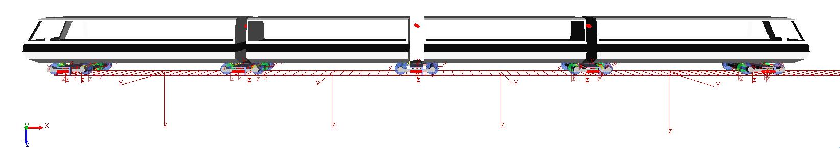
Fig. 1: Multibody model of the benchmark vehicle.

Two sets of experiments were performed. First, we solved a large number of sequences of nonlinear systems arising from wheel-rail contact in railway systems by the eight Srand variants based on the rules in Table 1. Second, we compared experimentally the best performing Srand variant and a standard Newton trust-region when embedded in the CONTACT algorithm.

The set of test problems used in the first part of the experiments was generated implementing the CONTACT algorithm in Matlab and using a standard trust-region Newton method for solving the arising nonlinear systems. Afterwards, a representative subset of the nonlinear systems was selected to form our problem set. Specifically, six sequences of nonlinear systems generated by the CONTACT algorithm and corresponding to six consecutive time instances for each track section (straight line, cycloid and curve) and for each velocity were selected. Such sequences are representative of the systems arising throughout the whole simulation and allow a fair analysis of Srand on nonlinear systems from a real application. Table 2 summarizes the features of the sequences: magnitude of the train velocity $v$, section of the route, time instances, number of nonlinear systems in the sequence, dimension $n$ of the systems (proportional to the number of mesh nodes in the potential contact area). A typical feature of the contact model is that $n$ increases as the velocity increases and when the train curves along the route (i.e., the track curvature increases). The total number of systems associated to ${v}=10\>m/s$ and ${v}=16\>m/s$ is 121 and 153 respectively.

${v}$($m/s$)	Track Section	Time Instances	Number of Systems	$n$
	Straight line	100-105	10	156
10	Cycloid	300-305	56	897
	Curve	450-455	55	1394
	Straight line	50-55	8	156
16	Cycloid	150-155	63	1120
	Curve	350-355	82	1394

Table 2: Sequences of nonlinear systems forming the first problem set.

6.3 Numerical results

In this section we present the performance of Srand algorithm. The results presented concern the solution of the sequences of nonlinear systems summarized in Table 2 and a comparison between the best performing Srand variant and a standard Newton trust-region method when embedded in the CONTACT algorithm.

Srand algorithm was implemented as described in Section 6.1 and with parameters

$$\beta_{\text{min}}=10^{-10},\ \ \beta_{\text{max}}=10^{10},\ \ \rho=10^{-4},\ \ \sigma=0.5,\ \ \eta_{k}=0.99^{k}(100+\|F_{0}\|^{2})\ \forall k\geq 0,$$

see [34]. The null vector $x_{0}=0$ was chosen as initial guess. A maximum number of iterations and $F$-evaluations equal to $10^{5}$ was imposed and a maximum number of backtracks equal to 40 was allowed at each iteration. The procedure was declared successful when

$$\|F_{k}\|\leq 10^{-6}.$$ (68)

A failure was declared either because the assigned maximum number of iterations or $F$-evaluations or backtracks is reached, or because $\|F\|$ was not reduced for 50 consecutive iterations.

We now compare the performance of all the variants of Srand method in the solution of the sequences of nonlinear systems in Table 2. Further, in light of the theoretical investigation presented in this work, we analyze in details the results obtained with BB1 and BB2 rule and support the use of rules that switch between the two steplengths.

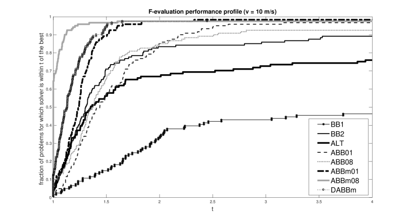
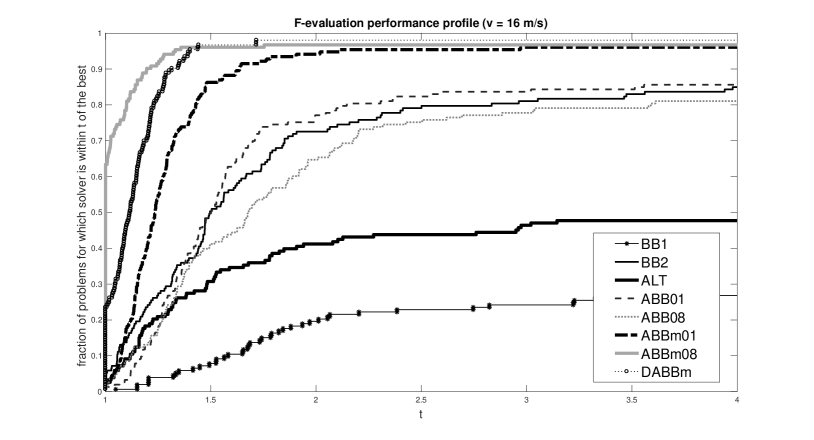
Fig. 2: $F$-evaluation performance profiles of Srand method. Upper: ${v}=10\>m/s$, Lower: ${v}=16\>m/s$.

Figure 2 shows the performance profiles [13] in terms of $F$-evaluations employed by the Srand variants for solving the sequence of systems generated both with ${v}=10\>m/s$ (121 systems) (upper) and with ${v}=16\>m/s$ (153 systems) (lower) and highlights that the choice of the steplength is crucial for both efficiency and robustness. The complete results are reported in Appendix B. We start observing that BB2 rule outperformed BB1 rule; in fact the latter shows the worst behaviour both in terms of efficiency and in terms of number of systems solved. Alternating $\beta_{k,1}$ and $\beta_{k,2}$ in ALT rule without taking into account the magnitude of the two scalars improves performance over BB1 rule but is not competitive with BB2 rule. On the other hand, the variants of Srand using adaptive strategies are the most robust, i.e., they solve the largest number of problems, and efficient. Specifically, comparing ABB, ABBm and DABBm rules, the most effective steplength selections are ABBm and DABBm. Using ABBm01 rule, 98.3% (2 failures) and 96.1% (6 failures) out of the total number of systems were solved successfully for ${v}=10\>m/s$ and ${v}=16\>m/s$ respectively; using ABBm08 rule, 98.3% (2 failures) and 96.7% (5 failures) of the total number of systems were solved successfully with ${v}=10\>m/s$ and ${v}=16\>m/s$ respectively; using the dynamic selection DABBm, the largest number of systems was solved successfully, i.e., 99.2% (1 failure) and 98% (3 failures) out the total number of systems with ${v}=10\>m/s$ and ${v}=16\>m/s$ respectively. Overall, ABBm08 rule gives rise to the most efficient algorithm for both velocity values and the profile related to BB2 rule is within a factor 2 of it in roughly the 80% and the 70% of the runs for ${v}=10\>m/s$ and ${v}=16\>m/s$, respectively.

Let us now focus on the performance Srand coupled with BB1 and BB2 rules. As a representative run of our numerical experience reported in Appendix B, we consider the nonlinear system arising with ${v}=16\>m/s$, at time $t=150$, iteration 2 of the CONTACT algorithm and iteration 2 of the TANG algorithm (system 150_2_2 in Table 7).

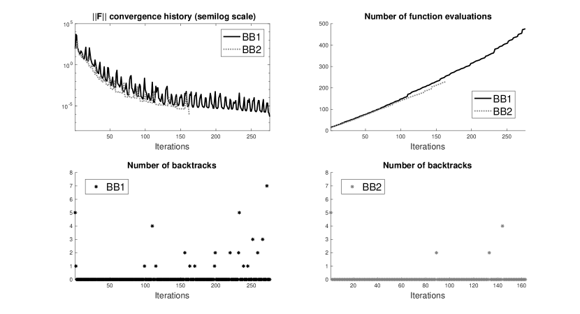
Fig. 3: Srand with BB1 rule vs Srand with BB2 rule on a single nonlinear system.

In the upper part of Figure 3 we display $\|F\|$ along iterations and the number of $F$-evaluations performed. We note that using the stepsize $\beta_{k,1}$ causes a highly nonmonotone behavior of $\|F\|$ and such behaviour is not productive for convergence; using BB1 rule 276 iterations and 476 $F$-evaluations are performed while using BB2 rule 163 iterations and 228 $F$-evaluations are required. The distinguishing feature of these runs is the high number of backtracks performed using $\beta_{k,1}$ at some iterations, as reported at the bottom part of the figure where the number of backtracks versus iterations is reported for both Srand variants. This behaviour is in accordance with the analysis in Section 4.1: since $\beta_{k,1}$ can be arbitrarily larger than $\beta_{k,2}$ in the indefinite case, the need to perform a large number of backtracks to enforce approximate norm decrease is likely to occur in case $\beta_{k,1}$ is taken as the initial steplength. Such observation supports the use of $\beta_{k,2}$; the benefit from using shorter steps is further shown by the performance of ABBm over ABB, the former tends to take shorter steps than the latter by exploiting the iteration history and results to be more effective.

We conclude our experimental analysis using a spectral residual method in the CONTACT algorithm. To this purpose, we compare two implementations of CONTACT algorithm which differ only in the nonlinear solver for the nonlinear systems arising in the TANG algorithm. The first implementation (CONTACT-NTR) uses a standard Newton trust-region method and the second one (CONTACT-DABBm) uses DABBm which turned out to be the more robust Srand version in the analysis above (see Figure 2). As a standard Newton trust-region method, we used the Matlab code proposed in [33]; default parameters were used and bound constraints on the unknown were dropped using the setting indicated in the code. The Jacobian matrix of $F$ was approximated by finite differences.

As a preliminary issue, we observe that the Jacobian matrices of $F$ are dense through the iterations; thus they cannot be formed as a low computational cost by finite difference procedures for sparse matrices [7]. We also observed in the experiments that the Jacobian matrices are nonsymmetric, do not have dominant diagonals and they are not close to diagonal matrices. For example, let us consider the Jacobian matrix of the system corresponding to speed ${v}=16\>m/s$, curve track section, instant $t=355$, iteration 2 of the CONTACT and iteration 4 of the TANG algorithm (355_2_4 in Table 8). It has dimension $292\times 292$ and, evaluated at the final iterate computed using ABBm08 rule, $96.18\%$ of its elements are nonzero. The structure of the Jacobian can be observed in Figure 4 where the absolute values of its elements are plotted in a logarithmic scale (the surface of the full matrix on the left and a plot of the row 146 on the right). This structure is observed along all the iterations of the nonlinear system solvers and is common to all sequences generated by the CONTACT algorithm.

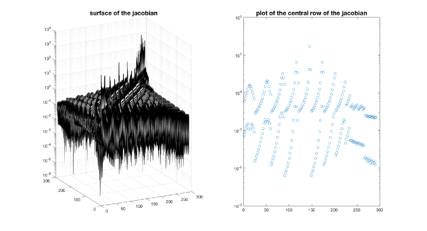
Fig. 4: Jacobian matrix: surface of the full matrix and plot of the central row (base 10 logarithm of the absolute values).

In our implementation, CONTACT algorithm terminated when the relative error between two successive values of the computed pressures dropped below $10^{-4}$ or a maximum of 20 alternating cycles between NORM and TANG was reached. Both nonlinear solvers were run until the stopping rule (68) is met. We ran CONTACT-NTR and CONTACT-DABBm over the whole track for both velocities, that is we considered the whole sequence of 500 time steps. CONTACT-NTR generated 3759 and 5353 nonlinear systems for ${v}=10\>m/s$ and ${v}=16\>m/s$, respectively and CONTACT-DABBm generated 4496 and 5494 nonlinear systems for the two velocities.

As a first remark, both procedures successfully solved the contact model described above and were reliable and accurate in the numerical simulation of wheel-rail interaction. Secondly, the use of the spectral residual method yields a gain in terms of time with respect to the use of a standard Newton method where finite difference approximation of Jacobian matrices is employed; this feature derives from the fact that spectral residual method is derivative-free and does not ask for the solution of linear systems. Figures 5 and 6 show the comparison of the two CONTACT implementations in terms of number of $F$-evaluations (excluding those needed to approximate the Jacobian matrices) and execution elapsed time. From the plots we observe that CONTACT-DABBm takes a larger number of $F$-evaluations than CONTACT-NTR but it is faster. Over the whole time interval, CONTACT-DABBm employs 1 hour, 19 mins and 2 hours, 28 mins to solve the generated nonlinear systems with ${v}=10\>m/s$ and ${v}=16\>m/s$, while CONTACT-NTR takes 7 hours and 49 mins and 12 hours and 41 mins, respectively.

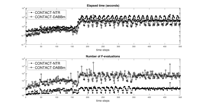
Fig. 5: Comparison between CONTACT-DABBm and CONTACT-NTR, ${v}=10\>m/s$: number of $F$evaluations and elapsed time in seconds (logarithmic scale).

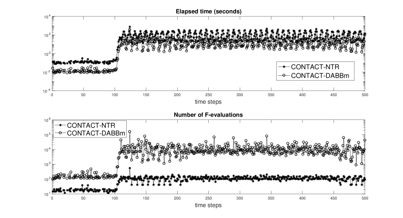
Fig. 6: Comparison between CONTACT-DABBm and CONTACT-NTR, ${v}=16\>m/s$: number of $F$evaluations and elapsed time in seconds (logarithmic scale).

7 Conclusions

The numerical behaviour of spectral residual methods for nonlinear systems strictly depends on the choice of the spectral steplength. Although most of the works on this subject make use of the stepsize $\beta_{k,1}$, known results on the spectral gradient methods for unconstrained optimization suggest that a suitable combination of the stepsizes $\beta_{k,1}$ and $\beta_{k,2}$ could be of benefit for spectral residual methods as well. This work aims to contribute to this study by providing a first systematic analysis of the stepsizes $\beta_{k,1}$ and $\beta_{k,2}$. Moreover, practical guidelines for dynamic choices of the steplength are derived from new theoretical results in order to increase both the robustness and the efficiency of spectral residual methods. Such findings have been extensively tested and validated on sequences of nonlinear systems arising in the solution of a contact wheel-rail model.

Acknowledgments

INdAM-GNCS partially supported the second, the third and the fourth author under Progetti di Ricerca 2019 and 2020.

Declarations

Conflict of interest The authors declare that they have no conflict of interest.

Funding Open access funding provided by Università di Bologna within the CRUI-CARE Agreement.

Appendix A Kalker’s contact model and CONTACT algorithm

We give an overview of the model and algorithm used to generate our set of nonlinear systems. Let bold letters represent vectors, the subscript $T$ denote a vector with components in the tangential $x$-$y$ contact place, the subscript $N$ denote the component of a vector in the normal $z$ contact direction. The contact problem between two elastic bodies [23, 24] determines the contact region $C$ inside the potential contact area $A_{c}$ (usually the interpenetration area between the wheel and rail contact surfaces), its subdivision into adhesion area $H$ and slip area $S$, and the tangential $\mathbf{p}_{T}$ and normal $p_{N}$ pressures such that the following contact conditions are satisfied:

$$\begin{array}[]{lll}\text{ normal problem}&{\text{ in contact }C:}&{e=0,\quad p_{N}\geq 0}\\ &{\text{ in exterior }E:}&{p_{N}=0,\quad e>0}\\ &{C\cup E=A_{c},}&{C\cap E=\emptyset}\\ \text{ tangential problem}&{\text{ in adhesion }H:}&{\|\mathbf{s_{T}}\|=0,\quad\|\mathbf{p_{T}}\|\leq g}\\ &{\text{ in slip }S:}&{\|\mathbf{s_{T}}\|\neq 0,\quad\mathbf{p}_{T}=-g\,\mathbf{s_{T}}/\|\mathbf{s}_{T}}\|\\ &{S\cup H=C,}&{S\cap H=\emptyset}\\ \end{array}$$ (69)

Above, $e$ is the deformed distance between the two bodies and, by definition, it holds $e=0$ and $p_{N}\geq 0$ in $C$. Referring to Figure 7, the region $E$ where $e>0$ is called the exterior area and $p_{N}=0$ therein. The potential contact area is such that $A_{c}=C\cup E$. The contact area $C$ is divided into the area of adhesion $H$ where the tangential component $\mathbf{s}_{T}$ of the slip vanishes, and the area $S$ of slip where $\mathbf{s}_{T}$ is nonzero. The slip $\mathbf{s}_{T}$ is the difference between the velocities of two homologous points belonging to deformed wheel and rail surfaces inside the contact area and is a function of the pressures $\mathbf{p}_{T}$ and $p_{N}$, $g$ is the traction bound (Coulomb friction model [23, 24]). Overall, the first three equations in (69) model the normal contact problem (computation of $p_{N}$ and of the shapes of the regions $C$ and $E$), whereas the last three equations describe the tangential contact problem (computation of $\mathbf{p}_{T}$, of local slidings $\mathbf{s}_{T}$ and of the shapes of the regions $H$ and $S$).

Let us consider the discretization of (69). Assuming that the contact patch is entirely contained in a plane, the region within which the potential contact area $A_{c}$ can be located is easily discretized through a planar quadrilateral mesh, see Figure 7. The coordinates of the center of each quadrilateral element are denoted $\mathbf{x}_{I}=\left(x_{I1},x_{I2},0\right)$ where the capital index $I$ identifies the specific element, say $I=1,\dots,N_{E}$. Also, the standard indices $i=1,2,3$, will indicate the vector components. For any element $I$ and any generic vector $\mathbf{w}_{I}=(w_{I1},w_{I2},w_{I3})$ associated to such mesh element, $w_{I1},w_{I2}$ are the components in the $x$-$y$ contact plane and $w_{I3}$ is the component in the normal contact direction $z$. Namely, $\mathbf{w}_{I,T}=(w_{I1},w_{I2})$ and $w_{I3}$ are the discrete counterparts of $\mathbf{w}_{T}$ and $w_{N}$, respectively.

Fig. 7: Local representation of the discretized contact area.

The discrete values of the elastic deformation $\mathbf{u}$ on the mesh nodes (i.e. the deformation of the elastic bodies in the contact area [23, 24]) are defined both at the current time instance $t$ and at the previous time instance $t^{\prime}$:

$$\mathbf{u}_{I}=\left(u_{Ii}\right)\hskip 2.84544pt\text{ at }\hskip 2.84544pt\left(\mathbf{x}_{I},t\right),\hskip 11.38092pt\mathbf{u}_{I}^{\prime}=\left(u_{Ii}^{\prime}\right)\hskip 2.84544pt\text{ at }\hskip 2.84544pt\left(\mathbf{x}_{I}+\mathbf{v}\left(t-t^{\prime}\right),t^{\prime}\right),$$ (70)

where $\mathbf{v}$ is the rolling velocity (i.e. the longitudinal velocity of the wheel) and $I$ is an arbitrary mesh element). Analogously, for the contact pressures $\mathbf{p}$ it holds

$$\mathbf{p}_{J}=\left(p_{Jj}\right)\hskip 2.84544pt\text{ at }\hskip 2.84544pt\left(\mathbf{x}_{J},t\right),\hskip 11.38092pt\mathbf{p}_{J}^{\prime}=\left(p_{Jj}^{\prime}\right)\hskip 2.84544pt\text{ at }\hskip 2.84544pt\left(\mathbf{x}_{J}+\mathbf{v}\left(t-t^{\prime}\right),t^{\prime}\right),$$ (71)

where $J$ is an arbitrary mesh element. According to the Boundary Element Method Theory [23, 24], the discretized displacements $\mathbf{u}_{I}$ can now be written as a function of the discretized contact pressures $\mathbf{p}_{J}$ through the discretized version of the problem shape functions, that is

$$u_{Ii}=\sum_{J=1}^{N_{E}}\sum_{j=1}^{3}A_{IiJj}p_{Jj},\hskip 5.69046pt\text{ with }A_{IiJj}:=B_{iJj}\left(\mathbf{x}_{I}\right),$$

and $B_{iJj}(\mathbf{x}_{I})$ are the discrete shape functions of the problem describing the effect of a contact pressure $\mathbf{p}_{J}$ applied to the element $J$ on displacement $\mathbf{u}_{I}$ of the node $I$ (see [23, 24]). The shape function $B_{iJj}$ usually depends on the problem geometry and the characteristics of the materials. An analogous expression can be derived for $u_{Ii}^{\prime}$. The elastic penetration $e$ can be calculated at each node $\mathbf{x}_{I}$ as

$$e_{I}=h_{I}+\sum_{J}A_{I3J3}p_{J3},$$

where $h_{I}$ is the discretization of the (known) undeformed distance between the two bodies, see [23, 24]. Similarly, the slip $\mathbf{s}_{T}$ can be discretized by setting

$$\mathbf{s}_{I,T}=\mathbf{c}_{I,T}+(\mathbf{u}_{I,T}-\mathbf{u}_{I,T}^{\prime})/(t-t^{\prime}),$$ (72)

where $\mathbf{c}_{I,T}$ is the discretization of the (given) rigid creep, that is the difference between the velocities of two homologous points belonging to the undeformed wheel and rail surfaces inside the contact area and thought of as rigidly connected to the bodies.

We observe that both $\mathbf{u}$ and $\mathbf{s}_{T}$ depend linearly on the pressures $\mathbf{p}$ and $\mathbf{p}^{\prime}$. Therefore, the discretization of equation $e=0$ in the norm problem (69) yields a linear system in the discretized normal pressures $(p_{I3})$ while the discretization of the nonlinear equation

$$\mathbf{p}_{T}=-g\,\mathbf{s}_{T}/\|\mathbf{s}_{T}\|,$$

in the tangential problem yields the nonlinear system

$$\mathbf{s}_{I,T}=-\|\mathbf{s}_{I,T}\|\mathbf{p}_{I,T}/g_{I},$$ (73)

with $\mathbf{p}_{I,T}=(p_{I1},p_{I2})$ being the unknown. When using the Coulomb-like friction model [23, 24], the friction limit function takes the form $g_{I}=f_{I}p_{I3}$, where $f_{I}$ is a given constant friction value.

The flow of Kalker’s CONTACT algorithm is displayed in Figure 8 [23, 24].

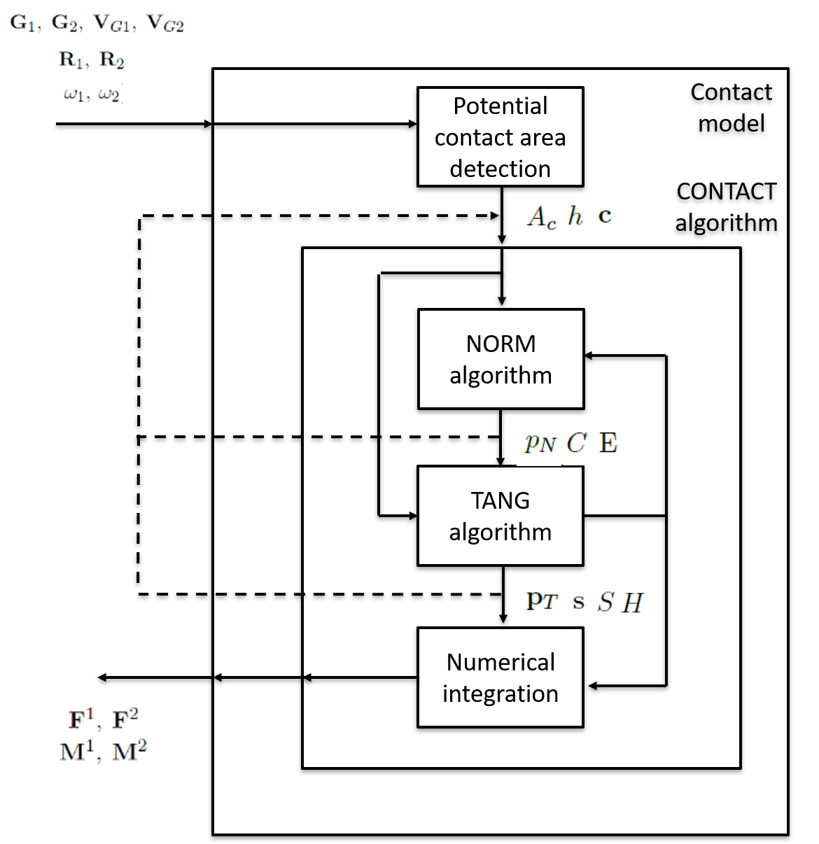
Fig. 8: The architecture of the Kalker’s CONTACT algorithm.

At each time step of time integration, the inputs of the CONTACT algorithm are the potential contact area $A_{c}$ (usually the interpenetration area between wheel and rail surfaces), the rigid penetration $h$ and the rigid local sliding $\mathbf{c}_{T}$ (inputs calculated, on turn, from the kinematic variables of the body: position and velocities of the gravity centers $\mathbf{G}_{1}$, $\mathbf{G}_{2}$, $\mathbf{V}_{G1}$, $\mathbf{V}_{G2}$, rotation matrices $\mathbf{R}_{1}$, $\mathbf{R}_{2}$ and angular velocities $\mathbf{\omega}_{1}$, $\mathbf{\omega}_{2}$) [23, 24]. All these kinematic quantities are calculated at each time step by the ODE solver of the Simpack Rail multibody environment [39]. NORM algorithm solves the normal contact problem and returns the contact area $C$, the non-contact area $E$, the normal contact pressures $p_{N}$. Then, TANG algorithm returns the sliding area $S$, adhesion area $H$, the tangential contact pressures $\mathbf{p}_{T}$ and local sliding $\mathbf{s}_{T}$. Repetitions of NORM and TANG algorithms are then performed to approximate accurately normal and tangential pressures $\mathbf{p}_{T}$, $p_{N}$. At the end of CONTACT algorithm, forces and torques exchanged by the contact bodies ($\mathbf{F}^{1}$, $\mathbf{F}^{2}$ and $\mathbf{M}^{1}$, $\mathbf{M}^{2}$) are computed by numerical integration and returned to the time integrator for proceeding in the dynamic simulation of the multibody system.

Appendix B Complete results

In this section we collect the complete runs which gave rise to the performance profiles in Figure 2. Results concern two velocities (${v}=10\,m/s$ in Tables 3-5 and ${v}=16\,m/s$ in Tables 6-8) and the three different track sections (straight line in Tables 3 and 6, cycloid in Tables 4 and 7 and curve in Tables 5 and 8). Given a sequence of nonlinear systems, we label a single system from the sequence as Time_Citer_Titer specifying the instant time (Time), the CONTACT iteration (Citer) and the TANG iteration (Titer). For each Srand variant applied to a system, we report the number of $F$-evaluations performed in case of convergence, or, in case of failure, the corresponding flag. We recall from Section 6.3 that a run is successful when $\|F_{k}\|\leq 10^{-6}$. A failure is declared either because the assigned maximum number of iterations or $F$-evaluations or backtracks is reached, or because $\|F\|$ was not reduced for 50 consecutive iterations. Such occurrences are denoted as ${\tt F_{it}}$ ${\tt F_{fe}}$, ${\tt F_{bt}}$, ${\tt F_{in}}$, respectively.

$v=10\ m/s$ - straight line
System	BB1	BB2	ALT	ABB		ABBm		DABBm
				$\tau=0.1$	$\tau=0.8$	$\tau=0.1$	$\tau=0.8$
101_1_2	69	59	74	75	59	71	57	69
101_2_2	382	148	248	295	205	174	198	220
103_1_2	37	31	35	37	30	37	31	34
103_2_2	37	31	35	37	30	37	31	34
104_1_2	36	36	37	36	38	36	39	38
104_2_2	36	36	37	36	38	36	39	38
105_1_2	39	38	39	39	38	39	39	39
105_1_3	77	69	82	79	70	82	67	74
105_2_2	40	37	39	40	38	40	39	39
105_2_3	74	73	86	75	70	75	67	76

Table 3: Number of function evaluations performed by Srand variants in the solution of nonlinear systems arising from time 100 to time 105 and corresponding to a straight line with velocity $10\ m/s$. In the first column we indicate the time step, the CONTACT and the TANG iteration.

	velocity $10\ m/s$ - cycloid
System	BB1	BB2	ALT	ABB		ABBm		DABBm	System	BB1	BB2	ALT	ABB		ABBm		DABBm
				$\tau=0.1$	$\tau=0.8$	$\tau=0.1$	$\tau=0.8$						$\tau=0.1$	$\tau=0.8$	$\tau=0.1$	$\tau=0.8$
300_1_2	178	128	137	145	149	174	133	163	303_2_2	${\tt F_{fe}}$	${\tt F_{in}}$	2196	${\tt F_{in}}$	${\tt F_{in}}$	1111	763	887
300_1_3	513	304	257	296	252	271	230	298	303_2_3	${\tt F_{fe}}$	1062	7400	1486	1413	911	722	798
300_1_4	569	402	290	464	350	460	278	299	303_2_4	${\tt F_{fe}}$	1713	10229	1780	1400	${\tt F_{in}}$	889	1054
300_2_2	343	203	266	229	194	209	168	204	303_2_5	${\tt F_{fe}}$	1424	23393	2053	1776	1201	1046	1358
300_2_3	16421	388	398	406	686	410	330	408	303_3_2	${\tt F_{fe}}$	926	6424	1352	806	896	814	821
300_3_2	357	223	248	257	205	225	187	232	303_3_3	${\tt F_{fe}}$	1318	6285	1508	886	1074	981	896
300_3_3	1650	385	368	432	530	462	339	499	303_3_4	${\tt F_{fe}}$	1279	14647	2295	1501	1244	959	1012
301_1_2	415	281	247	326	325	264	243	248	303_3_5	${\tt F_{fe}}$	${\tt F_{in}}$	17619	2353	${\tt F_{in}}$	1484	1311	1193
301_1_3	503	319	351	342	480	280	286	329	304_1_2	39075	962	815	643	504	714	447	491
301_1_4	582	442	281	380	376	344	291	305	304_1_3	${\tt F_{fe}}$	711	2891	860	1242	710	607	562
301_2_2	1127	286	298	271	430	310	284	297	304_1_4	${\tt F_{fe}}$	1524	3611	966	1423	785	515	752
301_2_3	630	414	367	388	430	322	313	337	304_2_2	725	366	381	393	416	300	311	317
301_2_4	758	345	372	408	355	363	319	386	304_2_3	65775	558	648	753	734	577	453	548
301_3_2	918	357	299	315	350	294	288	326	304_2_4	56953	709	1870	638	920	562	475	523
301_3_3	750	400	320	473	423	350	305	313	304_3_2	415	421	370	470	431	357	339	325
301_3_4	440	363	302	352	434	310	301	393	304_3_3	47176	533	2376	616	627	518	411	612
302_1_2	${\tt F_{fe}}$	743	3727	993	1022	558	457	495	304_3_4	86605	696	1180	709	603	557	468	488
302_1_3	${\tt F_{fe}}$	844	4067	1183	972	1068	670	678	305_1_2	796	270	311	302	323	329	242	364
302_1_4	${\tt F_{fe}}$	3546	25810	6171	2529	1735	1267	1342	305_1_3	339	293	270	271	294	288	243	310
302_2_2	634	444	417	552	539	431	332	376	305_1_4	430	342	301	354	335	307	230	309
302_2_3	27285	610	508	890	544	502	398	548	305_2_2	${\tt F_{fe}}$	${\tt F_{in}}$	2434	1401	800	${\tt F_{in}}$	1282	1208
302_2_4	${\tt F_{fe}}$	${\tt F_{in}}$	7325	1359	1951	927	853	693	305_2_3	${\tt F_{fe}}$	1110	2222	1713	1030	950	717	684
302_3_2	743	426	373	455	438	402	332	361	305_2_4	${\tt F_{fe}}$	${\tt F_{in}}$	842	1527	846	748	768	648
302_3_3	39825	739	502	869	616	459	401	463	305_2_5	${\tt F_{fe}}$	${\tt F_{in}}$	3329	1516	850	1332	573	597
302_3_4	${\tt F_{fe}}$	2245	7598	1141	938	1005	660	702	305_3_2	${\tt F_{fe}}$	980	6755	1524	${\tt F_{in}}$	920	1036	1518
303_1_2	22687	554	679	502	${\tt F_{in}}$	609	405	460	305_3_3	${\tt F_{fe}}$	${\tt F_{in}}$	5805	1829	756	694	634	579
303_1_3	33798	468	684	571	578	461	411	562	305_3_4	${\tt F_{fe}}$	871	2502	1363	997	857	716	648
303_1_4	${\tt F_{fe}}$	965	1163	734	669	653	524	613	305_3_5	${\tt F_{fe}}$	${\tt F_{in}}$	1786	1286	843	929	702	663

Table 4: Results for each system of the sequences generated in the cycloid section of the train track with velocity ${v}=10\ m/s$.

	velocity $10\ m/s$ - curve
System	BB1	BB2	ALT	ABB		ABBm		DABBm	System	BB1	BB2	ALT	ABB		ABBm		DABBm
				$\tau=0.1$	$\tau=0.8$	$\tau=0.1$	$\tau=0.8$						$\tau=0.1$	$\tau=0.8$	$\tau=0.1$	$\tau=0.8$
450_1_2	386	210	246	251	293	293	211	284	453_1_3	402	319	457	427	405	409	255	316
450_1_3	623	204	303	285	281	268	1580	1627	453_1_4	${\tt F_{fe}}$	${\tt F_{in}}$	2705	656	1285	996	611	544
450_2_2	29520	492	457	475	416	458	320	471	453_2_2	536	356	379	593	409	362	329	355
450_2_3	12031	428	433	412	458	415	309	387	453_2_3	${\tt F_{fe}}$	739	872	1030	557	726	${\tt F_{in}}$	560
450_3_2	13652	560	403	562	416	463	379	382	453_2_4	${\tt F_{fe}}$	1772	${\tt F_{in}}$	${\tt F_{in}}$	2018	1579	1535	${\tt F_{in}}$
450_3_3	11509	464	448	518	493	475	393	391	453_3_2	566	351	355	548	392	367	337	398
451_1_2	681	437	382	520	570	519	340	397	453_3_3	${\tt F_{fe}}$	558	598	796	617	612	536	568
451_1_3	${\tt F_{fe}}$	1218	4314	999	1564	868	613	1501	453_3_4	${\tt F_{fe}}$	${\tt F_{in}}$	${\tt F_{bt}}$	2308	${\tt F_{in}}$	1487	1187	1667
451_1_4	${\tt F_{fe}}$	3805	18920	1790	${\tt F_{in}}$	1305	1083	1334	454_1_2	147	153	165	139	153	137	138	150
451_2_2	324	274	329	264	264	263	210	250	454_1_3	207	175	206	229	192	194	154	175
451_2_3	${\tt F_{fe}}$	1652	1046	859	1304	691	520	595	454_1_4	2367	276	293	286	332	283	252	314
451_2_4	${\tt F_{fe}}$	1573	${\tt F_{in}}$	1260	${\tt F_{in}}$	1232	${\tt F_{in}}$	941	454_1_5	861	351	250	269	332	291	231	301
451_3_2	381	253	240	301	243	285	209	270	454_2_2	237	172	209	194	191	202	153	207
451_3_3	${\tt F_{fe}}$	3141	4232	660	801	640	606	635	454_2_3	413	279	211	288	315	240	254	280
451_3_4	${\tt F_{fe}}$	${\tt F_{in}}$	${\tt F_{in}}$	${\tt F_{in}}$	${\tt F_{in}}$	1042	936	888	454_2_4	901	363	209	256	307	262	227	261
451_4_2	358	296	321	279	295	268	213	263	454_3_2	259	204	204	183	198	183	157	183
451_4_3	${\tt F_{fe}}$	2108	901	688	729	676	597	639	454_3_3	469	317	329	273	290	244	251	265
451_4_4	${\tt F_{fe}}$	${\tt F_{in}}$	12872	1797	${\tt F_{in}}$	1093	905	821	454_3_4	450	302	231	277	297	254	229	270
452_1_2	66785	638	638	548	743	585	545	522	455_1_2	147	137	145	144	126	145	127	136
452_1_3	71198	701	725	535	789	489	552	508	455_1_3	212	184	203	219	166	226	166	196
452_1_4	45680	803	521	617	594	584	470	520	455_1_4	482	272	256	291	278	251	237	246
452_2_2	498	557	887	514	539	417	301	467	455_2_2	497	372	250	496	288	256	270	284
452_2_3	37679	608	714	474	672	456	425	454	455_2_3	563	393	473	641	340	436	357	348
452_2_4	40269	718	797	565	790	484	379	501	455_2_4	${\tt F_{fe}}$	840	5928	1544	929	1131	618	632
452_3_2	31230	433	451	438	517	345	405	354	455_3_2	341	270	268	391	392	302	238	282
452_3_3	41623	581	634	575	726	509	400	451	455_3_3	603	432	405	592	415	363	346	353
452_3_4	5592	477	658	572	570	457	407	470	455_3_4	${\tt F_{fe}}$	792	7505	1586	855	914	663	744
453_1_2	288	200	257	227	210	279	190	210

Table 5: Results for each system of the sequences generated in the curve segment of the train path with velocity ${v}=10\ m/s$.

velocity $16\ m/s$ - straight line
System	BB1	BB2	ALT	ABB		ABBm		DABBm
				$\tau=0.1$	$\tau=0.8$	$\tau=0.1$	$\tau=0.8$
50_1_2	60	45	53	52	47	52	46	49
50_2_2	53	44	51	54	48	54	48	53
50_3_2	53	44	51	48	48	48	48	53
52_2_2	75	78	53	76	75	101	61	91
52_3_2	89	78	53	76	88	112	61	91
55_1_2	65	66	66	83	66	80	62	72
55_2_2	69	79	60	76	61	73	67	71
55_3_2	69	79	60	80	61	73	67	71

Table 6: Number of function evaluations performed by Srand variants in the solution of nonlinear systems arising from time 50 to time 55 and corresponding to a straight line with velocity $16\ m/s$. In the first column we indicate the time step, the CONTACT and the TANG iteration.

	velocity $16\ m/s$ - cycloid
System	BB1	BB2	ALT	ABB		ABBm		DABBm	System	BB1	BB2	ALT	ABB		ABBm		DABBm
				$\tau=0.1$	$\tau=0.8$	$\tau=0.1$	$\tau=0.8$						$\tau=0.1$	$\tau=0.8$	$\tau=0.1$	$\tau=0.8$
150_1_2	985	297	330	366	357	351	278	343	153_1_3	${\tt F_{fe}}$	1173	1181	1162	1179	735	568	596
150_1_3	26886	569	512	612	555	487	419	437	153_1_4	${\tt F_{fe}}$	991	3881	1003	1590	1044	635	771
150_1_4	${\tt F_{fe}}$	967	3163	653	${\tt F_{in}}$	550	604	617	153_2_2	21846	475	603	688	532	578	396	446
150_1_5	${\tt F_{fe}}$	${\tt F_{in}}$	810	647	1549	614	510	710	153_2_3	${\tt F_{fe}}$	1149	3920	1316	1506	843	621	704
150_2_2	476	228	307	295	302	277	216	301	153_2_4	${\tt F_{fe}}$	1445	5035	1262	1272	1215	602	784
150_2_3	627	584	404	437	485	377	344	443	153_2_5	${\tt F_{fe}}$	772	4023	926	1576	1188	764	725
150_2_4	52373	585	479	494	730	438	391	435	153_3_2	1873	628	754	674	585	489	429	471
150_3_2	${\tt F_{fe}}$	1304	${\tt F_{in}}$	${\tt F_{in}}$	1777	2707	1237	911	153_3_3	${\tt F_{fe}}$	770	4768	1187	1882	941	699	860
150_3_3	${\tt F_{fe}}$	2498	${\tt F_{in}}$	${\tt F_{in}}$	${\tt F_{in}}$	2300	1973	1737	153_3_4	${\tt F_{fe}}$	1568	4872	923	1161	1173	678	709
150_3_4	${\tt F_{fe}}$	6214	${\tt F_{in}}$	${\tt F_{in}}$	${\tt F_{in}}$	3097	2576	${\tt F_{in}}$	153_3_5	${\tt F_{fe}}$	1226	5474	1145	1118	730	688	730
151_1_2	${\tt F_{fe}}$	${\tt F_{in}}$	5095	841	905	664	605	689	154_1_2	66851	776	3124	727	1033	585	534	527
151_1_3	${\tt F_{fe}}$	1114	5312	1421	1144	810	616	829	154_1_3	1031	386	513	467	681	433	310	346
151_1_4	${\tt F_{fe}}$	1454	8154	1630	3755	1125	1139	1046	154_1_4	18703	533	421	539	518	434	404	447
151_1_5	${\tt F_{fe}}$	3590	13111	2610	1435	1231	864	1043	154_2_2	947	319	312	420	357	341	294	356
151_2_2	${\tt F_{fe}}$	1337	12656	1333	3092	973	864	856	154_2_3	255	193	220	216	241	238	201	246
151_2_3	${\tt F_{fe}}$	3776	9599	1983	2198	1077	949	961	154_2_4	348	266	255	255	258	250	228	276
151_2_4	${\tt F_{fe}}$	3013	9073	1867	3551	1409	870	974	154_3_2	569	403	288	336	394	302	277	354
151_2_5	${\tt F_{fe}}$	5005	18543	1831	3662	1635	1270	1345	154_3_3	248	218	249	253	276	217	206	233
151_3_2	${\tt F_{fe}}$	${\tt F_{in}}$	7743	${\tt F_{in}}$	3893	${\tt F_{in}}$	939	803	154_3_4	346	318	278	281	271	267	239	250
151_3_3	${\tt F_{fe}}$	2293	9494	1383	1689	1080	809	982	155_1_2	${\tt F_{fe}}$	1161	5470	1151	987	824	718	859
151_3_4	${\tt F_{fe}}$	1235	7622	1416	1884	1075	856	941	155_1_3	${\tt F_{fe}}$	${\tt F_{in}}$	31313	4192	4270	1758	1401	1193
151_3_5	${\tt F_{fe}}$	4085	24983	1853	${\tt F_{in}}$	1509	1147	1330	155_1_4	${\tt F_{fe}}$	5839	19894	${\tt F_{in}}$	4182	1621	1729	1380
152_1_2	68856	822	1395	742	661	680	473	575	155_1_5	${\tt F_{fe}}$	${\tt F_{in}}$	${\tt F_{in}}$	${\tt F_{in}}$	${\tt F_{in}}$	1624	1351	1339
152_1_3	${\tt F_{fe}}$	682	4009	1153	1085	859	648	669	155_2_2	${\tt F_{fe}}$	1211	3754	1267	1275	764	651	635
152_1_4	${\tt F_{fe}}$	725	2905	986	1423	799	646	720	155_2_3	${\tt F_{fe}}$	${\tt F_{in}}$	${\tt F_{in}}$	2536	${\tt F_{in}}$	1658	1328	1273
152_2_2	21104	604	641	407	681	543	347	399	155_2_4	${\tt F_{fe}}$	1623	24770	3690	${\tt F_{in}}$	1626	1461	1427
152_2_3	80349	701	1082	636	845	632	476	610	155_2_5	${\tt F_{fe}}$	${\tt F_{in}}$	${\tt F_{bt}}$	${\tt F_{in}}$	${\tt F_{in}}$	1683	1715	1559
152_2_4	${\tt F_{fe}}$	1748	3725	1395	1034	873	590	849	155_3_2	${\tt F_{fe}}$	877	6004	990	882	795	567	818
152_3_2	20711	567	601	382	664	453	358	420	155_3_3	${\tt F_{fe}}$	${\tt F_{in}}$	23302	1784	${\tt F_{in}}$	${\tt F_{in}}$	1539	1238
152_3_3	75894	966	1098	522	898	639	535	627	155_3_4	${\tt F_{fe}}$	2895	32130	1953	${\tt F_{in}}$	1539	1739	1315
152_3_4	${\tt F_{fe}}$	1146	4114	848	1152	744	558	734	155_3_5	${\tt F_{fe}}$	${\tt F_{in}}$	${\tt F_{in}}$	6554	${\tt F_{in}}$	${\tt F_{in}}$	${\tt F_{in}}$	${\tt F_{in}}$
153_1_2	1281	408	589	512	495	472	400	397

Table 7: Results for each system of the sequences generated in the cycloid section of the train track with velocity ${v}=16\ m/s$.

	velocity $16\ m/s$ - curve
System	BB1	BB2	ALT	ABB		ABBm		DABBm	System	BB1	BB2	ALT	ABB		ABBm		DABBm
				$\tau=0.1$	$\tau=0.8$	$\tau=0.1$	$\tau=0.8$						$\tau=0.1$	$\tau=0.8$	$\tau=0.1$	$\tau=0.8$
350_1_2	424	320	308	359	366	297	284	286	352_4_5	${\tt F_{fe}}$	1132	7322	1252	${\tt F_{in}}$	921	${\tt F_{in}}$	724
350_1_3	${\tt F_{fe}}$	825	5650	826	905	771	540	687	353_1_2	468	357	398	482	342	352	307	357
350_2_2	308	208	220	244	261	243	197	247	353_1_3	887	640	588	557	441	508	446	456
350_2_3	${\tt F_{fe}}$	1322	3384	572	${\tt F_{in}}$	501	433	497	353_1_4	${\tt F_{fe}}$	695	4525	905	1369	781	625	656
350_2_4	${\tt F_{fe}}$	${\tt F_{in}}$	6845	1204	1523	746	790	718	353_1_5	${\tt F_{fe}}$	877	4670	793	1551	782	682	764
350_3_2	311	221	277	264	234	214	188	213	353_2_2	589	357	365	461	398	426	370	386
350_3_3	76754	${\tt F_{in}}$	885	639	666	491	416	481	353_2_3	47619	755	572	913	812	529	459	528
350_3_4	${\tt F_{fe}}$	${\tt F_{in}}$	6032	675	${\tt F_{in}}$	1141	761	647	353_2_4	${\tt F_{fe}}$	1143	3476	${\tt F_{in}}$	857	798	642	687
350_4_2	271	207	233	229	226	220	201	218	353_2_5	${\tt F_{fe}}$	1984	8598	1370	1700	${\tt F_{in}}$	867	1111
350_4_3	91233	764	3110	633	829	536	432	526	353_3_2	711	381	394	481	380	408	368	361
350_4_4	${\tt F_{fe}}$	1593	6301	722	${\tt F_{in}}$	637	${\tt F_{in}}$	751	353_3_3	65122	672	600	710	996	604	511	457
351_1_2	${\tt F_{fe}}$	1241	1625	920	913	772	597	538	353_3_4	${\tt F_{fe}}$	837	1623	815	1111	759	588	633
351_1_3	${\tt F_{fe}}$	1596	11134	1807	${\tt F_{in}}$	1374	1199	1090	353_3_5	${\tt F_{fe}}$	1250	6524	1233	1350	1110	915	855
351_1_4	${\tt F_{fe}}$	2272	20207	1862	${\tt F_{in}}$	1555	1217	1240	353_4_2	575	448	505	425	360	350	341	372
351_2_2	${\tt F_{fe}}$	1088	${\tt F_{in}}$	${\tt F_{in}}$	1207	1385	959	1050	353_4_3	57903	732	725	644	469	517	492	533
351_2_3	${\tt F_{fe}}$	2428	${\tt F_{in}}$	${\tt F_{in}}$	${\tt F_{in}}$	2185	1567	1825	353_4_4	${\tt F_{fe}}$	1030	932	873	1055	679	630	669
351_2_4	${\tt F_{fe}}$	5683	${\tt F_{in}}$	${\tt F_{in}}$	${\tt F_{in}}$	2421	2064	1636	353_4_5	${\tt F_{fe}}$	${\tt F_{in}}$	8112	1276	1502	980	904	967
351_2_5	${\tt F_{fe}}$	${\tt F_{in}}$	${\tt F_{in}}$	${\tt F_{in}}$	${\tt F_{in}}$	3192	2052	2770	354_1_2	313	229	219	320	261	265	187	253
351_3_2	${\tt F_{fe}}$	1261	12388	3742	1566	992	1166	876	354_1_3	502	323	369	398	337	318	267	342
351_3_3	${\tt F_{fe}}$	2029	${\tt F_{in}}$	${\tt F_{in}}$	${\tt F_{in}}$	${\tt F_{in}}$	${\tt F_{in}}$	1704	354_1_4	87446	710	4042	610	716	579	536	673
351_3_4	${\tt F_{fe}}$	2397	${\tt F_{in}}$	${\tt F_{in}}$	4270	2105	2074	1630	354_2_2	445	321	348	373	292	289	230	296
351_3_5	${\tt F_{fe}}$	${\tt F_{in}}$	${\tt F_{in}}$	${\tt F_{in}}$	${\tt F_{in}}$	2833	${\tt F_{in}}$	2635	354_2_3	1771	462	359	434	473	355	345	372
351_4_2	${\tt F_{fe}}$	1285	${\tt F_{in}}$	4846	1378	1262	1313	1028	354_2_4	${\tt F_{fe}}$	1054	4522	1052	1159	757	649	701
351_4_3	${\tt F_{fe}}$	1778	${\tt F_{in}}$	${\tt F_{in}}$	2581	2073	2144	1764	354_3_2	451	315	295	324	275	259	265	316
351_4_4	${\tt F_{fe}}$	${\tt F_{in}}$	${\tt F_{in}}$	${\tt F_{in}}$	${\tt F_{in}}$	2848	1794	1763	354_3_3	789	382	392	508	521	409	408	409
351_4_5	${\tt F_{fe}}$	${\tt F_{in}}$	${\tt F_{in}}$	${\tt F_{in}}$	${\tt F_{in}}$	${\tt F_{in}}$	3340	${\tt F_{in}}$	354_3_4	${\tt F_{fe}}$	913	3478	786	921	845	607	665
352_1_2	${\tt F_{fe}}$	1794	${\tt F_{bt}}$	5760	1636	1619	1933	1728	354_4_2	405	323	289	350	308	317	256	295
352_1_3	${\tt F_{fe}}$	3141	${\tt F_{bt}}$	3787	2872	1686	1495	1524	354_4_3	1776	497	363	452	338	399	333	370
352_1_4	${\tt F_{fe}}$	${\tt F_{in}}$	${\tt F_{in}}$	${\tt F_{in}}$	${\tt F_{in}}$	2334	1657	1721	354_4_4	${\tt F_{fe}}$	991	4561	830	1141	704	553	634
352_1_5	${\tt F_{fe}}$	${\tt F_{in}}$	${\tt F_{in}}$	${\tt F_{in}}$	${\tt F_{in}}$	2318	2846	1623	355_1_2	638	226	262	264	292	268	258	266
352_2_2	72375	676	1359	708	586	643	459	501	355_1_3	527	339	509	348	348	348	286	331
352_2_3	74955	801	878	794	718	857	481	519	355_1_4	35134	489	1201	464	525	477	382	408
352_2_4	${\tt F_{fe}}$	866	5116	1209	1071	837	648	746	355_2_2	346	222	252	246	243	221	194	242
352_2_5	${\tt F_{fe}}$	${\tt F_{in}}$	12683	1209	${\tt F_{in}}$	921	803	909	355_2_3	2303	480	396	402	357	313	261	358
352_3_2	59157	701	1249	712	652	687	420	589	355_2_4	41075	671	542	511	401	376	355	433
352_3_3	87628	1116	682	804	611	639	517	517	355_3_2	336	289	249	264	282	194	232	241
352_3_4	${\tt F_{fe}}$	808	6379	845	830	726	782	685	355_3_4	639	268	480	340	370	304	291	369
352_3_5	${\tt F_{fe}}$	1213	8333	1658	1133	863	697	781	355_3_5	24592	624	753	457	744	448	388	428
352_4_2	48585	603	818	679	775	668	460	528	355_4_2	363	214	268	226	261	261	203	221
352_4_3	79649	867	628	720	876	590	470	511	355_4_3	714	463	360	369	343	383	260	314
352_4_4	${\tt F_{fe}}$	${\tt F_{in}}$	4570	1046	1200	858	708	804	355_4_4	32137	404	700	411	532	562	367	451

Table 8: Results for each system of the sequences generated in the curve section of the train track with velocity ${v}=16\ m/s$.

References

- [1] Awwal, A. M., Kumam, P., Abubakar, A. B., Wakili, A., Pakkaranang, N.: A new hybrid spectral gradient projection method for monotone system of nonlinear equations with convex constraints. Thai J. Math. 66-88 (2018).
- [2] Barzilai, J., Borwein, J.: Two point step gradient methods. IMA J. Numer. Anal. 8, 141-148 (1988).
- [3] Birgin, E. G., Martinez, J. M., Raydan, M.: Spectral Projected Gradient Methods: review and Perspectives. J. Stat. Softw. 60(3) (2014).
- [4] Bonettini, S., Zanella, R., Zanni, L.: A scaled gradient projection method for constrained image deblurring. Inverse Probl. 25(1), 015002 (2009).
- [5] Carcasci C., Marini L., Morini B., Porcelli M.: A new modular procedure for industrial plant simulations and its reliable implementation. Energy, 94, pp. 380-390 (2016).
- [6] Crisci, S., Ruggiero, V., Zanni, L.:Steplength selection in gradient projection methods for box-constrained quadratic programs. Appl. Math. Comput. 356(1), 312-327 (2019).
- [7] Curtis, A.R., Powell, M.J.D., Reid, J.K.: On the estimation of sparse Jacobian matrices. IMA J. Appl. Math., 13, 117-119 (1974).
- [8] Dai, Y. H., Fletcher R.:Projected Barzilai-Borwein methods for large-scale box-constrained quadratic programming. Numer. Math. 100, 21-47 (2005).
- [9] Dai, Y. H., Hager, W., W., Schittkowski, K., Zhang, H.: The cyclic Barzilai-Borwein method for unconstrained optimization. IMA J. Numer. Anal. 26(3), 604-627 (2006).
- [10] De Asmundis, R., di Serafino, D., Riccio, F., Toraldo, G.: On spectral properties of steepest descent methods. IMA J. Numer. Anal. 33(4), 1416-1435 (2013).
- [11] Dennis Jr., J. E., Schnabel., R. B.: Numerical methods for unconstrained optimization and nonlinear equations. Prentice Hall Series in Computational Mathematics, Prentice Hall, Inc., Englewood Cliffs, NJ (1983).
- [12] di Serafino, D., Ruggiero, V., Toraldo, G., Zanni, L.: On the steplength selection in gradient methods for unconstrained optimization. Appl. Math. Comput. 318, 176-195 (2018).
- [13] Dolan E. D., Moré J. J.: Benchmarking optimization software with performance profiles. Math. Programming 91, 201-213 (2002).
- [14] Facchinei, F., Pang, J.S.: Finite-Dimensional Variational Inequalities and Complementarity Problems, Volume I. Springer Series in Operations Research, Springer, New York (2003).
- [15] Fletcher, R.: On the Barzilai-Borwein method. Optimization and control with applications, Appl. Optimizat. 96, 235-256, Springer, New York (2005).
- [16] Frassoldati, G., Zanni, L., Zanghirati, G.: New adaptive stepsize selections in gradient methods. J. Ind. Manag. Optim. 4(2), 299-312 (2008).
- [17] Glunt, W., Hayden, T., L., Raydan, M.: Molecular conformations from distance matrices. J. Comput. Chem. 14(1), 114-120 (1993).
- [18] Golub, G. H., Van Loan, C. F.: Matrix computations. Johns Hopkins Series in the Mathematical Sciences 3, Johns Hopkins University Press, Baltimore, MD (1983).
- [19] Gonçalves, M.L.N., Oliveira, F.R.: On the global convergence of an inexact quasi-Newton conditional gradient method for constrained nonlinear systems (2018).
- [20] Grippo, L., Lampariello, S., Lucidi, S.: A nonmonotone linesearch technique for Newton’s methods. SIAM J. Numer. Anal. 23, 707-716 (1986).
- [21] Grippo, L., Sciandrone, M.: Nonmonotone derivative-free methods for nonlinear equations. Comput. Optim. Appl. 37, 297-328 (2007).
- [22] Gu, G. Z., Li, D. H., Qi, L., Zhou, S. Z.: Descend directions of quasi-Newton methods for symmetric nonlinear equations. SIAM J. Numer. Anal. 40, 1763-1774 (2002).
- [23] Kalker, J.: Three-Dimensional elastic bodies in rolling contact. Kluwer Academic Print, Delft (1990).
- [24] Kalker, J., Jacobson, B,: Rolling contact phenomena. Springer Verlag, Wien (2000).
- [25] La Cruz, W., Raydan, M.: Nonmonotone spectral methods for large-scale nonlinear systems. Optim. Method Softw. 18, 583-599 (2003).
- [26] La Cruz, W., Martinez, J. M., Raydan, M.: Spectral residual method without gradient information for solving large-scale nonlinear systems of equations. Math. Comput. 75, 1429-1448 (2006).
- [27] La Cruz, W.: A projected derivative-free algorithm for nonlinear equations with convex constraints. Optim. Method Softw. 29, 24-41 (2014).
- [28] Li, D.H., Fukushima, M.: A derivative-free line search and global convergence of Broyden-like method for nonlinear equations. Optim. Method Softw. 13(3), 181-201 (2000).
- [29] Li, Q., Li, D. H.: A class of derivative-free methods for large-scale nonlinear monotone equations. IMA J. Numer. Anal. 31, 1625-1635 (2011).
- [30] Liu, J., Li, S.: Multivariate spectral dy-type projection method for convex constrained nonlinear monotone equations. J. Ind. Manag. Optim. 13, 283-295 (2017).
- [31] Marini, L., Morini, B., Porcelli, M.: Quasi-Newton methods for constrained nonlinear systems: complexity analysis and applications. Comput. Optim. Appl. 71, 147-170 (2018).
- [32] Mohammad, H., Abubakar A.,B.: A positive spectral gradient-like method for large-scale nonlinear monotone equations. Bull Comput. Appl. Math. 5, 99-115 (2017).
- [33] Morini, B., Porcelli, M.: TRESNEI, a Matlab trust-region solver for systems of nonlinear equalities and inequalities. Comput. Optim. Appl. 51, 27-49 (2012).
- [34] Morini, B., Porcelli, M., Toint, P.: Approximate norm descent methods for constrained nonlinear systems. Math. Comput. 87, 1327-1351 (2018).
- [35] Papini A., Porcelli M., Sgattoni C.: On the global convergence of a new spectral residual algorithm for nonlinear systems of equations. Boll. Unione Mat. Ital., 14, 367-378 (2021).
- [36] Raydan, M.: Convergence properties of the Barzilai and Borwein Gradient Method. PhD Thesis, Rice University (1991).
- [37] Raydan, M.: On the Barzilai and Borwein choice of step length for the gradient method. IMA J. Numer. Anal. 13, 321-326 (1993).
- [38] Raydan, M.: The Barzilai and Borwein gradient method for the large scale unconstrained minimization problem. SIAM J. Optimiz. 7, 26-33 (1997).
- [39] Simpack Multibody Simulation Software. Dassault Systemes GmbH.
- [40] Yu, Z., Lin, J., Sun, J., Xiao, Y., Liu, L., Li, Z.: Spectral gradient projection method for monotone nonlinear equations with convex constraints. Appl. Numer. Math. 59, 2416-2423 (2009).
- [41] Varadhan, R., Gilbert, P. D.: BB: an R package for solving a large system of nonlinear equations and for optimizing a high-dimensional nonlinear objective function. J. Stat. Softw. 32 (4) (2010).
- [42] Vollebregt, E. A. H.: Refinement of Kalker’s rolling contact model. Bracciali, Proceedings of the 8th International Conference on Contact Mechanics and Wear of Rail-Wheel Systems (CM2009), Firenze, 2009.
- [43] Vollebregt, E. A. H.: User guide for CONTACT, Rolling and sliding contact with friction. Technical Report TR09-03, version v15.1.1 (2015).
- [44] Zhang, L., Zhou, W.: Spectral gradient projection method for solving nonlinear monotone equations. J. Comput. Appl. Math. 196, 478-484 (2006).
- [45] Zhou, B., Gao, L., Dai, Y. H.: Gradient methods with adaptive step-sizes. Comput. Optim. Appl. 35(1), 69-86 (2006).