Evolution, Heritable Risk, and Skewness Loving

Abstract

Our understanding of risk preferences can be sharpened by considering their evolutionary basis. The existing literature has focused on two sources of risk: idiosyncratic risk and aggregate risk. We introduce a new source of risk, heritable risk, in which there is a positive correlation between the fitness of a newborn agent and the fitness of her parent. Heritable risk was plausibly common in our evolutionary past and it leads to a strictly higher growth rate than the other sources of risk. We show that the presence of heritable risk in the evolutionary past may explain the tendency of people to exhibit skewness loving today.

JEL Classification: D81, D91. Keywords: evolution of preferences, risk attitude, risk interdependence, long-run growth rate, fertility rate.
Final pre-print of a manuscript accepted for publication in Theoretical Economics.

1 Introduction

Our understanding of risk preferences can be sharpened by considering their evolutionary basis (see Robson and Samuelson, 2011, for a survey). This claim was advanced in the economics literature by Robson (1996), for example, who presented a model in which each agent lives a single period and faces a choice between lotteries over the number of offspring. (See also related models in Lewontin and Cohen, 1969; McNamara, 1995.) Some of the feasible lotteries involve aggregate risk (when all agents obtain the same realization). Robson (1996) showed that idiosyncratic risk (independent across individuals) induces a higher long-run growth rate (henceforth “growth rate”) than aggregate risk, and as a result natural selection should induce agents to be more risk averse with respect to aggregate risk.

This result has been put into an intriguing new light by Robatto and Szentes (2017) who reconsider the model in continuous time. In such a framework it is appealing to formulate both consumption and the production of offspring as rates. Once this is done aggregate risk becomes equivalent to idiosyncratic risk as long as fertility and mortality are age-independent. (See Robson and Samuelson, 2019, and Section 7 of this paper.)

The way in which idiosyncratic risk has been modeled in the previous literature captures well coin flips concerning fertility that only affect a particular individual. However, it is compelling that, in the evolutionary past, there were plausibly many cases in which the “outcome of the flip” persisted from parents to offspring. In this paper we capture this persistence by introducing a new source of risk, heritable risk, which is basically idiosyncratic risk, but allows a positive correlation between the fitness of a newborn agent and the fitness of her parent.

Heritable risk in this sense must have been common in the evolutionary past of human beings. Such risk is induced if the agent’s fitness is heritable due to imitation of the parent’s behavior or genetic inheritance. For example, a foraging technique in prehistoric hunter-gatherer societies would be inherited if an individual copied her parent’s technique. Alternatively, risk is heritable if the choice an individual makes is controlled genetically, and this gene is passed down from mother to daughter. The key properties are just: (1) there is a positive correlation between the fitness of an agent and that of her parent, and (2) by contrast, there is little correlation between the fitness of two randomly chosen agents in the population.

We show that this heritable risk yields a strictly higher growth rate than the other sources of risk. We derive this result in Robatto and Szentes’s (2017) setup, as it is more striking to see the advantage of heritable risk in a setup in which all other sources of risk are equivalent. It is relatively simple to show that heritable risk is also advantageous in other setups considered in the literature.

Highlights of the model

Consider a simple setup in which agents occasionally redraw a lottery over their consumption rate, and the realized consumption determines the fertility rate through a concave increasing function $\psi$. Specifically, assume that the lottery can yield a high consumption rate ($c_{h}$, inducing a fertility rate $r_{h}=\psi\left(c_{h}\right)$) with probability $q_{h}$ or a low consumption rate ($c_{l}$, inducing a fertility rate $r_{l}=\psi\left(c_{l}\right)$) with probability $q_{l}=1-q_{h}$. Each agent redraws her realized level of fertility at an annual rate of $\lambda$. For simplicity assume that there is no mortality. Our crucial departure from the existing literature is to assume that a newborn agent inherits the realized fertility rate of her parent and the values remain the same until either the parent or the offspring redraws their fertility rate.

Key result

Theorem 1 shows that the growth rate $x^{*}$ induced by heritable risk is both (1) strictly higher than the lottery’s expected fertility rate $\mu\equiv q_{\ell}\cdot r_{\ell}+q_{h}\cdot r_{h}$, but $x^{*}\rightarrow\mu$ as $\lambda\rightarrow\infty$, and (2) strictly below the highest realization $r_{h}$, but $x^{*}\rightarrow r_{h}$ as $\lambda\rightarrow 0$. To see the intuition behind (2), consider the case where $\lambda>0$ is small. The effect of the high realization of the heritable fertility rate gets compounded over time since parents with high fertility rates beget offspring with high fertility rates. Agents with high fertility rates therefore form an increasing fraction of the population over time, causing the overall growth rate to increase, and in the long run to be close to $r_{h}$.

Our result has two main implications: (1) heritable risk induces a higher growth rate than either aggregate risk or idiosyncratic risk (both of which induce a growth rate that is equal to the lottery’s expectation $\mu$), and (2) this difference in the growth rates is especially large when dealing with positively skewed lotteries (since the growth rate can be made close to $r_{h}$ in a way that is independent of the probability $q_{h}$).

One can interpret our result as follows. The long-run impact of risk interdependence depends on the “direction” of the interdependence (vertical or horizontal). The form of risk we introduce induces correlation between an agent’s outcome and her offspring’s outcome. This “vertical correlation” is helpful to the growth rate, as it allows successful families to have fast exponential growth. By contrast, this risk does not involve “horizontal correlation” of risk between agents of the same cohort, which would be harmful to the growth rate. The insight that vertical correlation increases the growth rate, but horizontal correlation decreases it, may be applicable in other domains of economics and finance.

Risk attitude

We assume that individuals in our evolutionary past had different types, and that the agent’s type determines her risk attitude—in particular, how the agent chooses between a risky consumption option and a safe one. An agent is likely to have the same type as her parent due to genetic inheritance. Occasionally, new types are introduced into the population following a genetic mutation. Observe that the population share of agents of the type that induces the highest long-run growth rate will grow, until, in the long run, almost all agents are of this type.

In Section 5 we show that our key result implies that the type with the highest growth rate is (1) risk averse with respect to most lotteries over consumption (due to the concavity of the function $\psi$ relating consumption and fertility), but (2) risk loving with respect to sufficiently positively skewed lotteries. Since biological types evolve slowly, it is likely that this risk attitude persists in modern times, even though the birth rate may no longer be increasing in the consumption rate. This finding fits the stylized empirical fact that people, although being in general risk averse, are skewness loving. That is, people like lotteries involving a small probability of winning a high prize. (See, for example, Golec and Tamarkin, 1998; Garrett and Sobel, 1999.)

Structure

The rest of the paper is organized as follows. Section 2 informally presents the essence of our key result. The model is presented in Section 3. Section 4 formally presents our key result. In Section 5 we discuss the implications of our result for attitudes to risk. Section 6 extends our baseline model by allowing dependency between redraws of heritable risk within each of a number of dynasties, with independence across dynasties, which seems plausible in various applications. We show that this extension does not affect our results for infinite populations. By contrast, this structure can affect the growth rate of finite populations, which we investigate by numerical simulations. We discuss several additional related references in Section 7 and conclude in Section 8.

2 Informal Treatment of Key Result

The following example conveys the gist of our key result. Consider three populations, each having a random fertility rate (which is independent of the agent’s age) with the same marginal distribution. Each population has a probability $q_{\ell}$ of having a low fertility rate of $r_{\ell}$, and a probability $q_{h}=1-q_{\ell}$ of having a high fertility rate of $r_{h}$. For notational compactness, we now take as implicit the dependence of fertility on consumption rates $c_{i},i=\ell,h$. For simplicity, we focus on fertility, so that there is no mortality. The source of risk is independent across populations.

In Population 1 risk is idiosyncratic; that is, the fertility rate of each agent is independent of the fertility rate of all other agents in the populations and, in particular, of her parent’s fertility rate. Applying the law of large numbers, the number of agents in Population 1 at time $t$ is equal to $N(t)=e^{\left(q_{\ell}\cdot r_{\ell}+q_{h}r_{h}\right)\cdot t}$, where $N(0)=1$, and the annual growth rate is $\frac{1}{t}\cdot\ln N(t)=q_{\ell}\cdot r_{\ell}+q_{h}r_{h}\equiv\mu$.

In Population 2 risk is aggregate. There are two states: $\ell$ and $h$. In state $\ell$, all agents have fertility rate $r_{\ell}$, and in state $h$, all agents have fertility rate $r_{h}$. There is a continuous probability rate $\lambda$ that the state is redrawn. If it is, the fertility rate is $r_{\ell}$ with probability $q_{\ell}$ and $r_{h}$ with probability $q_{h}$. What is the (long-run) growth rate of the population exposed to this aggregate risk? If $N(t)$ is the population at time $t$, and $N(0)=1$, it follows that

$$\frac{\ln N(t)}{t}=\frac{r_{\ell}\cdot({\text{time in state }}\ell)+r_{h}\cdot(\text{time in state }h)}{t}\longrightarrow q_{\ell}\cdot r_{\ell}+q_{h}\cdot r_{h}=\mu,$$

as ${t\rightarrow\infty}$, given the evident ergodicity of the process. Thus, as shown in Robatto and Szentes (2017), both idiosyncratic risk and aggregate risk induce the same growth rate.

We introduce a novel form of risk in Population 3, called heritable risk. Each agent redraws her heritable birth rate independently of all other agents at a rate $\lambda$, and at each redraw the agent gets a fertility rate $r_{\ell}$ or $r_{h}$ with probability $q_{\ell}$ or $q_{h}=1-q_{\ell}$, respectively (independently of all other events). The previous literature makes an implicit assumption that each offspring is given a fresh draw, and so all offspring are equivalent and evolutionary success entails simply counting these undifferentiated offspring. By contrast, suppose that each offspring inherits the realized fertility rate of the parent. Since offspring are now differentiated, the value of these offspring varies with type and simply counting them is inadequate. Our key result shows that in this case the growth rate is strictly higher than the expectation $\mu$, and indeed converges to $r_{h}$ as $\lambda\rightarrow 0$.

To understand the gist of the argument, consider a simplified alternative setup in which redraws arrive deterministically and in synchrony every $\tau$ periods, which is comparable to an arrival rate of $\lambda=1/\tau$. As before, the redrawn values of different agents are independent. On each draw, a share $q_{\ell}$ of the agents get $r_{\ell}$ and the remaining agents get $r_{h}$. If the initial population is of size $1$, then, after a time $k\cdot\tau$, the population is $N(k\cdot\tau)=(q_{\ell}\cdot e^{r_{\ell}\cdot\tau}+q_{h}\cdot e^{r_{h}\cdot\tau})^{k},$ so that

$$\frac{1}{k\cdot\tau}\ln N(k\cdot\tau)=\frac{1}{\tau}\cdot\ln(q_{\ell}\cdot e^{r_{\ell\cdot}\tau}+q_{h}\cdot e^{r_{h}\cdot\tau})\equiv\bar{g}(\lambda).$$

It follows that the growth rate of the population, $\bar{g}\left(\lambda\right)$, is decreasing in $\lambda$, $\bar{g}(\lambda)\rightarrow r_{h}$ if $\lambda\rightarrow 0$ ($\tau\rightarrow\infty$), and $\bar{g}(\lambda)\rightarrow\mu\equiv q_{\ell}\cdot r_{\ell}+q_{h}\cdot r_{h}$, if $\lambda\rightarrow\infty$ ($\tau\rightarrow 0$). This, in particular, implies that the growth rate is strictly higher than the lottery’s expectation $\mu$, which is the growth rate induced by either idiosyncratic risk or aggregate risk with the same marginal distribution.

Recall that $x^{*}$ is the growth rate in the general model. What Theorem 1 shows, more precisely, is that $x^{*}>\mu$ and $x^{*}>r_{h}-\lambda$. This latter result implies that $x^{*}\rightarrow r_{h}$ as $\lambda\rightarrow 0$, given $x^{*}<r_{h}$. Figure 1 illustrates our result for the values $r_{h}=5\%$, $r_{l}=0\%$, and $q_{h}=10\%$; i.e., for a binary lottery that yields a high annual birth rate of $5\%$ with probability $10\%$ and a zero birth rate with probability $90\%$. When risk is either idiosyncratic or aggregate the (long-run) growth rate is equal to the expected birth rate $\mu=0.5\%$. Theorem 1 (and the informal argument above) shows that when the risk is heritable the growth rate is strictly larger than $\mu$. The figure also draws the exact growth rate induced by heritable risk according to the explicit formula presented in Claim 1 (in Appendix C) for binary lotteries. As can be seen from the figure, when the redraw rate $\lambda$ is very small (resp., large) with respect to $r_{h}$, then the growth rate is slightly above $r_{h}-\lambda$ (resp., $\mu$).

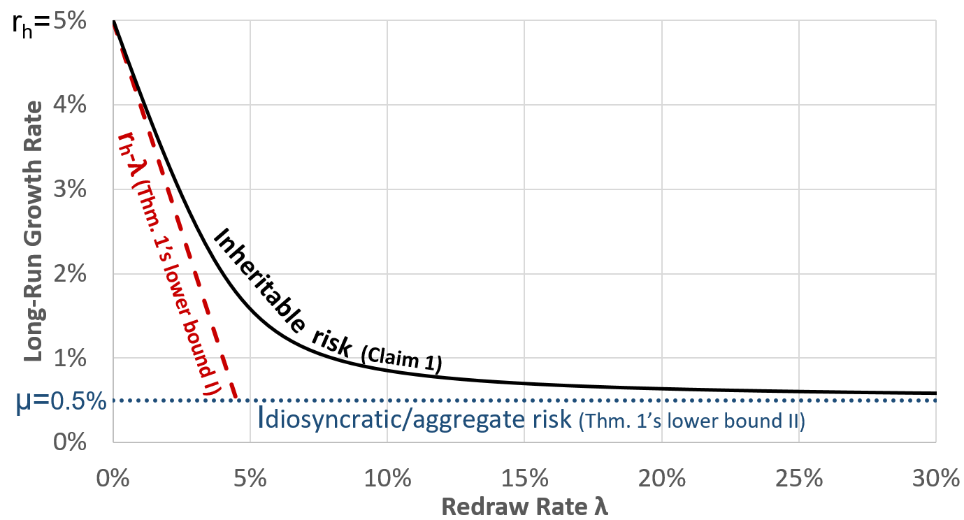
Figure 1: Long-Run Growth Rate for a Binary Lottery ( $r_{h}=5\%$, $r_{l}=0\%$, and $q_{h}=10\%$).

3 Model

Consider a continuum population of an initial mass one. Time is continuous, indexed by $t\in\mathbb{R}^{+}$. To simplify matters, we assume that reproduction is asexual. The growth process depends on the parameters $\left(\delta,\left(X,q_{x},\lambda_{x}\right),\left(Y,q_{y},\lambda_{y}\right),\left(Z,q_{z},\lambda_{z}\right)\right)$, as described below.

In what follows, we first present an intuitive description of Poisson processes on the individual level that incorporate the probability of each agent dying, giving birth, and changing her birth rate (parts (i) below). We then specify the corresponding exact evolution of the large population that is assumed in our model (parts (ii) below).

1. (i) We suppose intuitively that each agent experiences a constant Poisson death rate $\delta\geq 0$ that is independent of all other random variables and, in particular, of all components of the birth rates.

   (ii) We assume precisely that, in each infinitesimal period of time between $t$ and $t+dt$, a fraction $\delta\cdot dt$ of the population dies, where this fraction is uniform across all components of the birth rate.

Each individual $i$ at time $t$ has a birth rate $\boldsymbol{b}^{i}\left(t\right)=\boldsymbol{x}^{i}\left(t\right)+\boldsymbol{y}^{i}\left(t\right)+\boldsymbol{z}\left(t\right)$ with three components. These components are constructed as follows:

1. (i) The random variable $\boldsymbol{x}^{i}\left(t\right)\geq 0$ is the heritable component of the birth rate. A newborn agent obtains the heritable birth rate of her parent. We assume that the random variable $\boldsymbol{x}^{i}$ has a finite support $X=supp\left(\boldsymbol{x}\right)=\left\{x_{1},...,x_{n}\right\}$, where $x_{1}<...<x_{n}$ and $n\geq 2$. The function $q_{x}:X\rightarrow(0,1),\leavevmode\nobreak\ \sum_{x\in X}q_{x}=1,$ assigns a probability to each $x\in X.$ Intuitively, in each infinitesimal period of time $dt$ each agent has a probability of $\lambda_{x}\cdot dt$ of redrawing her heritable birth rate (where $\lambda_{x}>0$), and these redrawing events are independent of all other events.

   (ii) The precise assumptions on the heritable component are as follows. Suppose that $w(t)$ is the total population at time $t$ and $w_{k}(t)$ is the mass of agents who are endowed with heritable component $x_{k}$. Then the rate of increase of $w_{k}(t)$ is

   $$\frac{dw_{k}(t)}{dt}=w_{k}(t)x_{k}-\lambda_{x}w_{k}(t)+\lambda_{x}w(t)q_{x}(x_{k})-\delta w_{k}(t).$$ (1)

   The first term expresses the increase in $w_{k}(t)$ due to offspring who are endowed with $x_{k}$. This captures the key characteristic of heritable risk that all offspring are endowed with the same component $x_{k}$ as their parent. Since this term is independent of $\lambda_{x}$, it will follow that $w_{k}(t)$ grows at rate $x_{k}-\delta$ when $\lambda_{x}\rightarrow 0$. The second term expresses the loss from $w_{k}(t)$ of those agents who redraw. The third term represents the increase due to all agents from $w(t)$ (including those from $w_{k}(t)$) who redraw and obtain $x_{k}$. The final term represents the loss from $w_{k}(t)$ due to death.

2. (i) The random variable $\boldsymbol{y}^{i}(t)\geq 0$ is the idiosyncratic component of the birth rate. The idiosyncratic birth rate of an agent is independent of all other random variables governing the birth rates in the population. The random variable $\boldsymbol{y}^{i}$ has a finite support $Y=supp\left(\boldsymbol{y}\right)=\left\{y_{1},...,y_{n_{y}}\right\}$. The function $q_{y}:Y\rightarrow(0,1],\leavevmode\nobreak\ \sum_{y\in Y}q_{y}=1$, assigns a probability to each $y\in Y.$ In each infinitesimal period of time $dt$ each agent has a probability of $\lambda_{y}\cdot dt$ of redrawing her idiosyncratic birth rate, and these redrawing events are independent of all other events.

   (ii) The precise assumption is that the idiosyncratic component within any group of agents always reflects the distribution $q_{y}$. That is, the share of agents with idiosyncratic outcome $y_{\ell}$, for example, in the group of agents with heritable outcome $x_{k}$ is exactly equal to $q_{y}(y_{\ell})$ for any time $t\geq 0$. This implies that the idiosyncratic component in any group of agents with any heritable component $x_{k}$ is exactly equal to the expectation $\mu_{y}$.

3. The aggregate component of the birth rate $\boldsymbol{z}\left(t\right)\geq 0$ can be handled more straightforwardly since all agents in the population share this aggregate rate. We assume that the random variable $\boldsymbol{z}^{i}$ has a finite support $Z=supp\left(\boldsymbol{z}\left(t\right)\right)=\left\{z_{1},...,z_{n_{z}}\right\}$. The function $q_{z}:Z\rightarrow(0,1],\leavevmode\nobreak\ \sum_{z\in Z}q_{z}=1,$ assigns a probability to each $z\in Z.$ At time $t=0$ the aggregate birth rate $\boldsymbol{z}\left(0\right)$ is randomly determined according to the distribution $q_{z}$. In each infinitesimal period of time between $t$ and $t+dt$ a new random value of the aggregate birth rate is drawn independently (according to $q_{z}$) with a probability of $\lambda_{z}\cdot dt$, where $\lambda_{z}>0$. This aggregate birth rate applies to all individuals in the entire population equally.

4 Key Result

Let ${w}\left(t\right)$ denote the mass of the population at time $t$. We normalize ${w}\left(0\right)=1$. We say that the growth process of ${w}\left(t\right)$ given by $\left(\delta,\left(X,q_{x},\lambda_{x}\right),\left(Y,q_{y},\lambda_{y}\right),\left(Z,q_{z},\lambda_{z}\right)\right)$ has an equivalent (long-run) growth rate $g\in\mathbb{R}$ if and only if

$$lim_{t\rightarrow\infty}\frac{\ln{w}\left(t\right)}{t}=g,{\text{ almost surely.}}$$

Let $\mu_{x}=\sum_{k}x_{k}\cdot q_{x}\left(x_{k}\right)$ (resp., $\mu_{y}=\sum_{k}y_{k}\cdot q_{y}\left(y_{k}\right)$, $\mu_{z}=\sum_{k}z_{k}\cdot q_{z}\left(z_{k}\right)$) be the expectation of the heritable (resp., idiosyncratic, aggregate) birth rate. We show that the equivalent growth rate is the sum of four components: $g=f\left(X,q_{x},\lambda_{x}\right)+\mu_{y}+\mu_{z}-\delta.$ The results on the idiosyncratic and aggregate components of the overall growth rate accord with the existing literature (Robatto and Szentes, 2017), namely, these components are equal to $\mu_{y}$ and $\mu_{z}$, respectively. The novel part of the result is that the heritable birth component satisfies

$$f\left(X,q_{x},\lambda_{x}\right)\in\left(\max\left(\mu_{x},x_{n}-\lambda_{x}\right),x_{n}\right).$$

That is, the heritable birth component is always larger than $\mu_{x}$, and it cannot be more than $\lambda_{x}$ away from the highest realization $x_{n}$. The first property shows that the desirability of heritable risk is that it induces a higher growth rate than comparable aggregate or idiosyncratic risk. The second property shows that the highest realization of the heritable risk has a substantial influence, regardless of how low is its probability. That is, a lottery in which $x_{n}>\lambda_{x}$ induces a growth rate of at least $x_{n}-\lambda_{x}$ regardless how small $q_{x}(x_{n})$ and $\mu_{x}$ might be.

The intuition is that the distribution of the heritable birth rate in the population converges to a distribution $p\in\Delta\left(X\right)$ that first-order stochastically dominates $q_{x}$. This is because, at each point in time, agents with a high heritable birth rate tend to have more offspring and these offspring share the parent’s heritable birth rate. Hence, in a steady state, the share of agents with a high heritable birth rate is strictly higher than $q$. Higher values of $\lambda$ reduce this effect, as the offspring redraw more rapidly a new value for their heritable birth rate (according to $q_{x}$).

The final claim is that $f\left(X,q_{x},\lambda_{x}\right)$ increases following a mean-preserving spread of the heritable birth rate. The intuition is that a mean preserving spread increases the high $x_{k}$’s while decreasing the low $x_{k}$’s, and there is a net gain from this due to the over-representation of high $x_{k}$-agents in the steady-state distribution.

Theorem 1.

Let $\left(\delta,\left(X,q_{x},\lambda_{x}\right),\left(Y,q_{y},\lambda_{y}\right),\left(Z,q_{z},\lambda_{z}\right)\right)$ be a growth process. Then its equivalent growth rate is equal to $g=f\left(X,q_{x},\lambda_{x}\right)+\mu_{y}+\mu_{z}-\delta,$ where, setting $f\left(X,q_{x},\lambda_{x}\right)=x^{*}$ for compactness, $x^{*}$ is the unique positive solution of

$$x^{*}=\lambda_{x}\sum_{k=1}^{n}\frac{q_{k}\cdot x_{k}}{\lambda_{x}+x^{*}-x_{k}}\in\left(\max\left(\mu_{x},x_{n}-\lambda_{x}\right),x_{n}\right),$$

with $q_{k}\equiv q_{x}\left(x_{k}\right)$ for each $k\in\left\{1,..,n\right\}$. It follows that $x^{*}\rightarrow\sum_{k=1}^{n}q_{k}x_{k}=\mu_{x}$ as $\lambda_{x}\rightarrow\infty$ and $x^{*}\rightarrow x_{n}$ as $\lambda_{x}\rightarrow 0.$

Moreover, if $\left(X^{\prime},q^{\prime}_{x}\right)$ is a mean-preserving spread of $\left(X,q_{x}\right)$, then $f\left(X^{\prime},q_{x^{\prime}},\lambda_{x}\right)>f\left(X,q_{x},\lambda_{x}\right)$.

Sketch of proof; The full proof is in Appendix A.

Since the novel result here concerns heritable risk, let us suppose, for simplicity, that there is no aggregate risk, idiosyncratic risk, or mortality. Suppose further that the size of the population at time $t$ is $w(t)$ and that a steady-state fraction $p_{k}$ of this population has birth rate $x_{k}$. The net increase in each infinitesimal period $dt$ of those agents with birth rate $x_{k}$ is then $p_{k}\cdot x_{k}\cdot w\left(t\right)\cdot dt$ (offspring born to parents with a birth rate $x_{k}$ who inherit this rate) minus $(p_{k}-q_{k})\cdot\lambda_{x}\cdot w\left(t\right)\cdot dt$. (Note that $\lambda_{x}\cdot w\left(t\right)\cdot dt$ agents have redrawn a fresh value for the heritable birth rate, and the share of $x_{k}$-agents among them has changed from $p_{k}$ to $q_{k}$.) The increase in the total mass of agents is $\sum_{k}p_{k}\cdot x_{k}\cdot w\left(t\right)\cdot dt$ (the sum of offspring born to parents with each birth rate). The equilibrium value of $p$ should match the ratio of the net increase of agents with a high heritable birth rate to the net increase of the population, such that

$$p_{k}=\frac{\left(p_{k}\cdot x_{k}+(q_{k}-p_{k})\cdot\lambda_{x}\right)\cdot w\left(t\right)\cdot dt}{\sum_{k}p_{k}\cdot x_{k}\cdot w\left(t\right)\cdot dt}=\frac{p_{k}\cdot x_{k}+(q_{k}-p_{k})\cdot\lambda_{x}}{\sum_{k}p_{k}\cdot x_{k}\cdot}.$$

Solving for $p_{k}$ yields (where $x^{*}\equiv\sum_{k}p_{k}\cdot x_{k}$):

$$p_{k}=\frac{\lambda_{x}\cdot q_{k}}{\lambda_{x}+x^{*}-x_{k}}.$$ (2)

This solution assumes that $p_{k}$ is positive for all $k$ so that $x^{*}>x_{n}-\lambda_{x}.$ Next we multiply each $k$-th equation by $x_{k}$ and sum to an equation in one unknown:

$$x^{*}=\sum_{k}\frac{x_{k}\cdot\lambda_{x}\cdot q_{k}}{\lambda_{x}+x^{*}-x_{k}}.$$ (3)

Observe that in the domain $x^{*}>x_{n}-\lambda_{x}$ the LHS (resp., RHS) is increasing (resp., decreasing) in $x^{*}$, which implies that there exists a unique solution $x^{*}>x_{n}-\lambda_{x}$ to Eq. (3). Substituting this solution in Eq. (2) yields the unique steady-state distribution $p$. From Eq. (3) it follows that

$$x^{*}=\sum_{k}\frac{x_{k}\cdot q_{k}}{1+\frac{x^{*}-x_{k}}{\lambda_{x}}}\rightarrow\sum_{k}x_{k}\cdot q_{k},$$ (4)

as $\lambda_{x}\rightarrow\infty.$ Since $x^{*}\in(x_{n}-\lambda_{x},x_{n}),$ it is also immediate that $x^{*}\rightarrow x_{n}$ as $\lambda_{x}\rightarrow 0.$

The final claim is proved as follows. Eq. (3) can be written as

$$\boldsymbol{E}_{\boldsymbol{x}}\left[\frac{\boldsymbol{x}\cdot\lambda}{\lambda+x^{*}-\boldsymbol{x}}\right]=x^{*},$$ (5)

where $\boldsymbol{x}$ is the random variable $\left(X,q_{x}\right)$. The fact that $\frac{\boldsymbol{x}\cdot\lambda}{\lambda+x^{*}-\boldsymbol{x}}$ is a convex function of $\boldsymbol{x}$ implies that it increases following a mean-preserving spread. This, together with the fact that it is decreasing in $x^{*}$, implies that in order to maintain Eq. (5) following a mean-preserving spread, the growth rate $x^{*}$ must increase. ∎

5 Risk Attitude

We suppose that individuals in a large population may have different types, where the type represents the agent’s risk attitude—in particular, how the agent chooses between a risky consumption option and a safe one. An agent has the same type as her parent. Occasionally, new types may be introduced into the population as genetic mutations. Observe that the population share of agents that are endowed with the type that induces the highest long-run growth rate for its practitioners will grow, until, in the long run, almost all agents are of this type. For example, suppose that there are two types $\theta,\theta^{\prime}$ in the population, each with an initial frequency of 50% that induce growth rates $g(\theta),g(\theta^{\prime})$, respectively. After time $t$ the share of agents having type $\theta$ will be $\frac{e^{g\left(\theta\right)t}}{e^{g\left(\theta\right)t}+e^{g\left(\theta^{\prime}\right)t}},$ which converges to one as $t\rightarrow\infty$, if $g\left(\theta\right)>g\left(\theta^{\prime}\right)$. See Robson and Samuelson (2011) and the citations therein, for a more detailed argument of why natural selection induces agents to have types that maximize the long-run growth rate.

Now consider a setup in which agents face choices between various alternatives, where each alternative corresponds to a lottery over the consumption rate. We assume that the birth rate is a concave increasing function of consumption, given by $\psi:\boldsymbol{R}^{+}\rightarrow\boldsymbol{R}^{+}$. To simplify the presentation, assume that the birth rate is entirely heritable; the result remains qualitatively the same if the birth rate induced by consumption has all three risk components (heritable, idiosyncratic, and aggregate). We now argue that a growth-rate-maximizing type induces agents (1) to be risk averse with respect to most lotteries over consumption, and, yet, (2) to strictly prefer some fair lotteries that are sufficiently skewed. Thus, natural selection should induce agents to have a risk attitude combining risk aversion and skewness loving.

For simplicity, assume that an agent faces choices among lotteries over consumption $\left(C,q\right)$ with a finite support $C$, where $c>0$ for all $c\in C.$ Suppose probabilities are assigned by $q:C\rightarrow[0,1],\sum_{c\in C}q(c)=1$. Let $m=\max\left\{c\in C\right\}$ be the maximal possible realization and let $\bar{c}=\sum_{c\in C}q(c)\cdot c$ be the mean. For any fixed lottery, we show that, once $\psi$ is sufficiently concave, the constant consumption rate of $\bar{c}$ will induce a higher long-run growth rate than the lottery $\left(C,q\right)$. This explains why the growth-rate-maximizing type should induce the agents to be risk averse with respect to most lotteries, when $\psi$ is sufficiently concave. Consider, for example, the function $\psi(c)=c^{\beta}$ for $\beta\in(0,1]$. Theorem 1 shows that the individual prefers the lottery $\left(C,q\right)$ to the mean $\bar{c}$ when $\beta=1$ so that $\psi(c)=c$. However, if $\beta$ is small enough this preference is reversed. This is formalized in the following proposition that shows that, given any lottery over consumption, the individual will prefer the mean consumption to the lottery if $\beta$ is small enough.

Proposition 1.

Suppose that $\psi(c)=c^{\beta}$ for $\beta\in(0,1]$. Then, given any gamble $\left(C,q\right)$, the mean $\bar{c}=\sum_{c\in C}q\left(c\right)\cdot c$ induces a higher growth rate than the lottery $(C,q)$, if $\beta>0$ is close enough to $0$.

Proof See Appendix B.

On the other hand, for a fixed function $\psi(c)$, if the lottery $\left(C,q\right)$ is sufficiently skewed—i.e., if $m$ is high enough and $q\left(m\right)$ is low enough so that $\psi(m)-\lambda_{x}>\psi(\bar{c})$—then the lottery induces a strictly higher growth rate than the constant consumption rate of $\bar{c}$. This follows from Theorem 1 since the lottery’s long-run growth rate is bounded from below by $\psi(m)-\lambda_{x}$. This implies that growth-rate-maximizing agents would prefer a sufficiently positively skewed lottery to its expectation.

The above argument suggests that natural selection has induced people to be generally risk averse and sometimes skewness loving. As biological types evolve slowly, it seems likely that this risk attitude persists in modern times, in which, arguably, the birth rate is no longer increasing in the consumption rate. Thus, our findings fit the stylized fact that people, although being in general risk averse, are skewness loving, in the sense of being risk loving with respect to lotteries involving a small probability of winning a high prize (e.g., buying state lottery tickets; see Golec and Tamarkin, 1998; Garrett and Sobel, 1999).

6 An Extended Model: Dynasties

In our baseline model, the event of an agent redrawing her heritable birth rate is independent of her parent’s redrawing event. In various environments, it seems plausible that members of a dynasty may change their heritable birth rate together, while remaining independent of other dynasties. For example, if heritable risk is induced by a foraging technique or a geographical location, and environmental changes affect the effectiveness of the foraging technique, then an entire dynasty of agents (who use the same foraging technique or live in the same geographical location) may simultaneously change their heritable birth rate.

In this section we extend our baseline model by introducing dynasties, and allowing dependency between redraws of heritable risk within each dynasty. We show that this extension does not affect our results for infinite populations. By contrast, this structure can affect the growth rate of finite populations, which we investigate by numerical simulations.

Extended model

In what follows we extend our baseline model to a continuum of dynasties. We adopt the same notation as in the baseline model. The processes according to which agents die, are born, and change their idiosyncratic and aggregate birth components remain the same as in the baseline model. Importantly, each offspring is born into the same dynasty as her parent.

Let $[0,1]$ be the set of dynasties, where each agent $i$ in the initial population (of mass one) lives in a different dynasty $i\in[0,1]$. Each dynasty is initially endowed with a heritable birth rate according to the distribution $q_{x}$. Formally, we assume that the mass of dynasties having heritable birth component $x_{k}\in X$ is equal to $q_{x}(x_{k}).$ The heritable birth component of each agent is tied to the heritable birth component of all members of her dynasty.

There are two processes that change the heritable birth component of agents. We begin with an intuitive description of two Poisson processes that change the heritable birth component: migration and a dynasty’s redraw. We then specify the corresponding exact evolution of the distribution of the heritable birth component as the product of these two processes.

1. Migration: Intuitively, in each infinitesimal time $dt$ each agent has a probability of $\lambda_{m}\cdot dt$ (where $\lambda_{m}\geq 0$) to leave her dynasty and move to a new random dynasty (distributed uniformly in the set of all dynasties [0,1]). These migration events are independent of all other events. Following the migration, the agent is endowed with the heritable birth component of her new dynasty.

2. Dynasty’s redraw: Intuitively, in each infinitesimal time $dt$ each dynasty $j\in[0,1]$ has a probability of $\lambda_{r}\cdot dt$ to redraw a fresh value for its heritable birth component. These redrawing events are independent of all other events. When a dynasty redraws its heritable component it changes the heritable component of all agents living in that dynasty.

Next, we formulate the precise dynamics of the mass of agents $w_{k}(t)$ who are endowed with the heritable component $x_{k}$ that is induced by the combined effect of migration and a dynasty’s redraws. The rate of increase of $w_{k}(t)$ is

$$\frac{dw_{k}(t)}{dt}=w_{k}(t)x_{k}-\lambda_{m}w_{k}(t)+\lambda_{m}w(t)q_{x}(x_{k})-\lambda_{r}w_{k}(t)+\lambda_{r}w(t)q_{x}(x_{k})-\delta w_{k}(t).$$ (6)

The first and final terms are identical to Eq. (1) of the baseline model. The first term expresses the increase in $w_{k}(t)$ due to offspring who are endowed with $x_{k}$. The final term represents the loss from $w_{k}(t)$ due to death.

The second and third terms express the impact of migration. The second term ($-\lambda_{m}w_{k}(t)$) is the loss from $w_{k}(t)$ of agents who migrate out of dynasties with heritable component $x_{k}$. The third term ($\lambda_{m}w(t)q_{x}(x_{k})$) represents the increase due to all agents from $w(t)$ (including those from $w_{k}(t)$) who migrate into dynasties with heritable component $x_{k}$.

The fourth and fifth terms express the impact of redraws of dynasties. The fourth term ($-\lambda_{r}w_{k}(t)$) represents the loss from $w_{k}(t)$ of agents who live in dynasties with heritable component $x_{k}$ that redraw a fresh draw. Finally, the fifth term ($\lambda_{r}w(t)q_{x}(x_{k})$) represents the increase due to all agents from dynasties (including dynasties that already had $x_{k}$) that draw a fresh value of heritable component $x_{k}$.

Observe that Eq. (6) is equivalent to Eq. (1) of the basic model except that $\lambda_{x}$ is replaced with $\lambda_{m}+\lambda_{r}$. That is, the dynamics of $w_{k}(t)$ in the extended model is exactly the same as in the baseline model with $\lambda_{x}=\lambda_{m}+\lambda_{r}$. As the impact of the heritable component on the growth rate is exactly captured by $w_{k}(t)$, this implies that all of our results hold in this extended setup with dynasties.

Ever-growing population with dying dynasties

Consider a simple case in which: (1) $\lambda_{m}=0$, i.e., agents never migrate, and each dynasty is an isolated subpopulation, (2) all risk is heritable, (3) the growth rate predicted by the continuum model is positive, and (4) an aggregate birth rate with the same marginal distribution induces a negative growth rate. For example, assume that the heritable birth rate of each dynasty is randomly chosen to be either $x_{l}=0\%$ or $x_{h}=2\%$ with equal probability, that there is a constant death rate of $\delta=1.4\%$, and that the redrawing rate of the heritable risk by each dynasty is given by $\lambda_{r}=2\%$. Theorem 1 and Claim 1 imply that this heritable birth rate induces a positive growth rate of 0.014%, while if the birth rate were induced by aggregate risk with the same distribution, then the growth rate would be negative: $-0.4\%=\left(0.5\cdot 0\%+0.5\cdot 2\%\right)-1.4\%$.

Each dynasty is a completely isolated subpopulation with risk that is essentially aggregate within the subpopulation. Thus, each dynasty is doomed to extinction since it has a negative growth rate of $-0.4\%$. This yields a seemingly paradoxical result: the entire population grows exponentially, while each of its dynasties eventually becomes extinct. Such a result holds with a continuum of dynasties. Although each dynasty eventually dies, in each finite time there is still a continuum of surviving dynasties with a large realized growth rate, such that the growth rate of the entire population can be positive.

The intuition behind this result can be illustrated more clearly in a simple alternative setup in which each dynasty in each period can be either successful or go extinct with equal probability. A successful dynasty increases its size by a factor of 4 in each period. Observe that the expected size of each dynasty after $t$ period is $2^{t}$, which is the product of a tiny probability of $0.5^{t}$ of the dynasty surviving and the very large size of the dynasty ($4^{t}$), conditional on surviving. If the population includes a continuum of mass one of dynasties, then (by applying an exact law of large numbers) after $t$ periods the size of the population is $2^{t}$ (with probability one), and this population is concentrated on a continuum of a small mass of $0.5^{t}$ of surviving large dynasties. Thus, the population’s size converges to infinity, even though the share of surviving dynasties converge to zero. By contrast, if the number of dynasties were finite (instead of a continuum), then after a sufficiently long finite time, the population’s size would eventually be zero with probability one.

Finite populations

The result of an ever-growing population in which each dynasty is eventually doomed cannot happen when the number of dynasties is finite. Since each dynasty is doomed to extinction, so too is the overall population. However, the fact that the mean size of each subpopulation is growing implies that the overall population may grow significantly in the interim. As the finite model converges to the continuum model, this initial growth phase becomes more and more prolonged, and the inevitable ultimate demise of the population is postponed indefinitely.

When there is no migration, a large finite population tends to ultimately put all its eggs in one basket. That is, the distribution of the finite population over its subpopulations tends to become very unequal, often concentrated in just one subpopulation. Such large subpopulations hold up the mean, which is the growth rate found here. Once the population is concentrated like this, however, doom is inevitable because the heritable risk of a large subpopulation, essentially, becomes an aggregate risk since it affects a large share of the entire population.

Migration introduces a new element to these observations. In the finite model migration has a distinct effect from that of the redraw rate. If some subpopulations grow large, and others shrink, migration acts to redistribute the population. This means that the population can exploit the numbers in the large subpopulations, while diversifying the risk. These observations motivate the simulations described below.

6.1 Numerical Analysis of Finite Populations

In this section we present simulations that test whether our theoretical results for continuum populations hold for finite populations.

Description of the Simulation

The simulation is a discrete-time version of the extended model (with dynasties) described above. Specifically, the basic time step of the simulation is one year, and we replace each continuous Poisson rate with the respective independent per-year probability (e.g., an annual birth rate of $2\%$ is replaced with an independent probability of $2\%$ of each agent giving birth in each year). The Python code (contributed by Renana Heller) is included in the online supplementary material.

We describe here the results of 150 simulation runs, which comes from 15 runs of 10 different parameter combinations. In each simulation run, the initial population includes 3,000 agents that are initially randomly allocated to 300 dynasties. The aggregate birth rate and the idiosyncratic birth rate are both equal to zero (i.e., $\mu_{y}=\mu_{z}=0$). The heritable birth rate in each dynasty is randomly chosen to be either $x_{l}=0\%$ or $x_{h}=2\%$ with equal probabilities (i.e., $q=0.5$). We set the total annual rate at which each agent switches the heritable birth rate to be $\lambda_{m}+\lambda_{r}=2\%$. We set the annual death rate at 1.4%, which implies that the theoretical prediction for a continuum population (see Claim 1 in Appendix C) is that: (1) the share of agents with a high heritable birth rate converges to about $71\%$, and (2) the annual long-run growth rate will be about $0.014\%$. A naive prediction that treats heritable risk as if it were aggregate risk predicts a long-run growth rate of $-0.4\%=\left(0.5\cdot 0\%+0.5\cdot 2\%\right)-1.4\%$. Due to technical constraints and time limits we stopped each simulation run after (1) 20,000 years have passed, (2) the population size increases by 300-fold to 1,000,000 or more, or (3) the population size decreases by 300-fold to 10 or less (henceforth, extinction). The various simulation runs study 10 different ratios $\frac{\lambda_{m}}{\lambda_{r}}$ of the migration rate relative to the dynastic risk redrawing rate (while maintaining $\lambda_{m}+\lambda_{r}=2\%$): 0.01, 0.02, 0.05, 0.1, 0.25, 0.5, 1, 2, 4, 10.

Numerical Results

Figure 2 presents four representative simulation runs with ratios: 0.01 ($\lambda_{m}=0.02\%$, $\lambda_{r}=1.98\%$), 0.05 ($\lambda_{m}=0.1\%$, $\lambda_{r}=1.9\%$), 0.25 ($\lambda_{m}=0.4\%$, $\lambda_{r}=1.6\%$), and 1 ($\lambda_{m}=\lambda_{r}=1\%$).

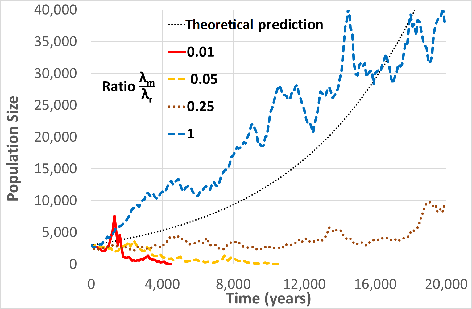
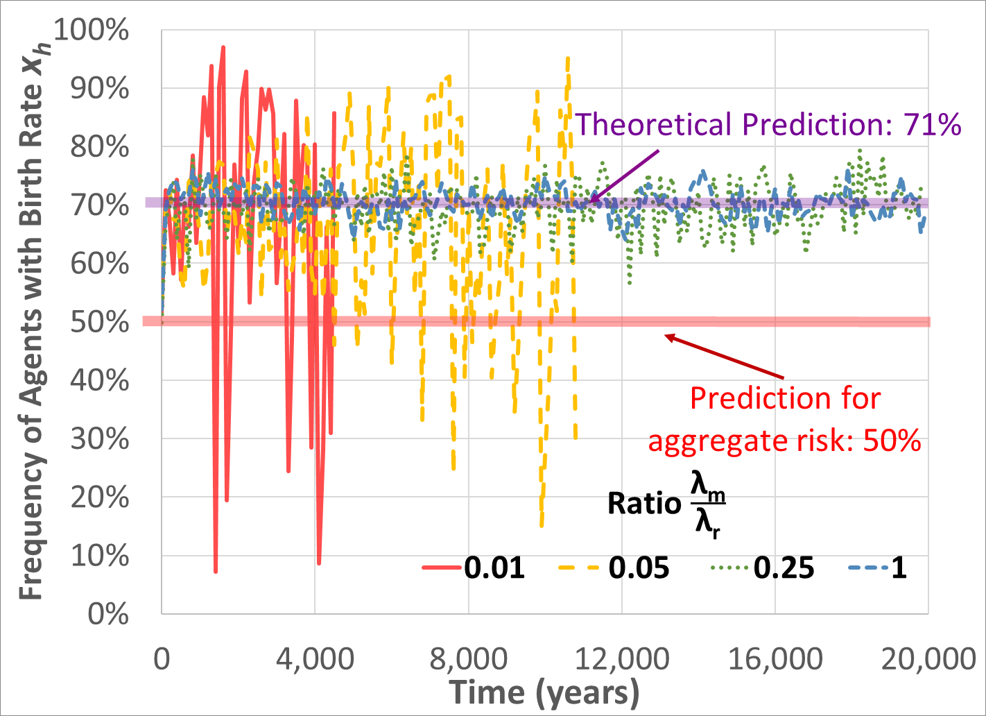
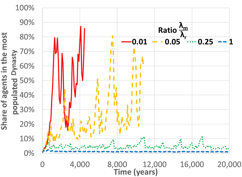
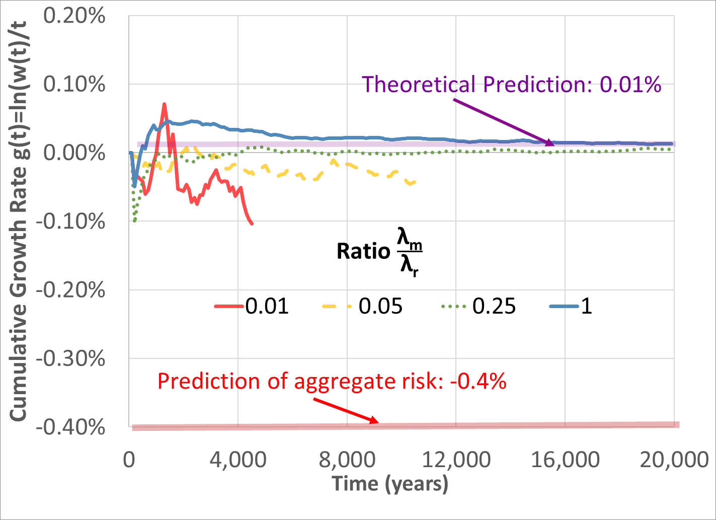
Figure 2: Representative Simulation Runs for four Ratios of $\frac{\lambda_{m}}{\lambda_{r}}$

The top-left panel of Figure 2 shows the dynamics of the total population in each of the four simulation runs. The top-right panel shows how the frequency of agents that are endowed with a high heritable birth rate evolves. The bottom-left panel shows the percentage of agents that live in the most populated dynasty (among the 300 dynasties). The bottom-right panel shows the cumulative growth rate up to time $t$ in each year (i.e., it shows $g\left(t\right)=\frac{\ln\left(w\left(t\right)\right)}{t}$).

The figure shows that when the ratio $\frac{\lambda_{m}}{\lambda_{r}}$ is small (0.01 or 0.05), dynastic risk has similar properties to aggregate risk. The low rate of migration implies that a couple of “successful” dynasties (which happen to have had a high heritable birth rate for a long time) contain most of the population. This causes the heritable risk, essentially, to be aggregate. The frequency of agents with a high heritable birth rate has large fluctuations, since a single change of the heritable birth rate of the most populated dynasty has a large impact on this frequency. This is shown in the top-right panel. The cumulative growth rate (bottom-right panel) is initially positive, but after a couple of thousand years it becomes negative and starts converging to the negative growth predicted by aggregate risk, until the population becomes extinct (top-left panel).

By contrast, Figure 2 shows that when the ratio $\frac{\lambda_{m}}{\lambda_{r}}$ is 0.25 (resp., 1), then the theoretical prediction for the continuum case becomes relatively (resp., very) accurate for the finite population. When the migration rate is sufficiently high, a “successful” dynasty spreads its offspring to many other dynasties, staving off extinction. The bottom-left panel shows that the frequency of agents living in the most populated dynasty is at most 10% (resp., 2%). This implies that the share of agents with a high heritable birth rate has a relatively (resp., very) small fluctuations around Claim 1’s predicted value of about 71%, as can be seen in the top-right panel. The cumulative growth rate (bottom-right panel) converges to the positive value of 0.01%, as predicted in Claim 1, as is shown in the top-left panel.

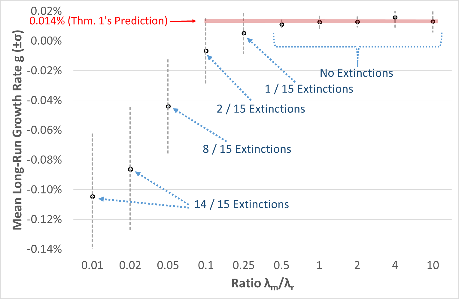
Figure 3: Mean Long-Run Growth Rate for each Ratio of $\frac{\lambda_{m}}{\lambda_{r}}$

The black points describe the mean growth rate of 15 simulation runs for each ratio of $\frac{\lambda_{m}}{\lambda_{r}}$. The vertical bars show intervals of one standard deviation on each side of the mean. The labels describe how many simulation runs ended in an extinction of the population.

Figure 3 presents the mean long-run growth rate obtained in the 15 simulation runs for each of the ten ratios of $\frac{\lambda_{m}}{\lambda_{r}}$. The results show that conclusions drawn from the four representative simulation runs presented in Figure 2 are indeed valid for the entire set of 150 simulation runs.

7 Discussion

Asexual reproduction

Our model, like the related literature, makes the simplifying assumption that reproduction is asexual, where offspring are identical to the parent. Similar results should hold if reproduction were sexual and haploid, where a single genetic variant—an allele—that determines choice is inherited with probability $1/2$ from either parent. That is, if a particular choice in a gamble is currently favored, this advantage will hold in a muted form if offspring inherit it through haploid sex. Further, if the gene controlling choice is evident to a mate, homophily—a preference for like individuals—would accentuate this advantage, bringing the model back to the asexual case.

Horizontal and vertical correlation

An insight of our model is that vertical correlation increases the growth rate, but horizontal correlation decreases it. Horizontal correlation is called within-generation bet hedging by Lehmann and Balloux (2007). Vertical correlation is called the multiplayer effect by McNamara and Dall (2011) who study a non-overlapping generations model in which an asexual species breeds annually in one of a large number of breeding sites. Each site can be either good (high expected number of offspring) or bad. In each generation each site changes its type with probability less than 0.5. Each animal observes a noisy signal about the quality of the site in which it was born, and it has to choose whether to stay or to migrate to a new site. McNamara and Dall show that when the signal is sufficiently noisy, it is best for nature to induce each animal to ignore the signal, and always stay in its birth site because the mere fact that the animal was born in the site makes it more likely that the site is good.

Additive separability

Our model assumes that the various component of risk are additively separable. This assumption clearly facilitates the analysis. It permits a direct comparison of the implications of the three types of risk. Separability seems intuitively unlikely to be crucial to the results. At the least, there ought to be approximate results for a general non-separable criterion and small aggregate, heritable and idiosyncratic components. Further, it seems that it would be possible to allow for arbitrary aggregate shocks with heritable and idiosyncratic shocks conditional on the aggregate state, much as in Robson (1996).

Age structure

Recently, a different approach was applied by Robson and Samuelson (2019) to show that risk interdependence matters in a continuous-time setting (see also related results in Robson and Samuelson, 2009). Specifically, they show that adding age structure to Robatto and Szentes’s (2017) setting (i.e., allowing the fertility rate to depend on the agent’s age) implies that interdependence of risk influences the growth rate. By contrast, the present paper shows that interdependence of risk is important for the induced growth rate in a hierarchical population, even when the age structure is trivial, but still in a continuous-time setting. It would be interesting for future research to study the implications of heritable risk in age-structured populations.

Migration between fragmented habitats

Our numerical analysis suggests an important advantage to connecting isolated small habitats of an endangered species. The related existing literature (e.g., Burkey, 1999; Smith and Hellmann, 2002) shows that having several isolated small habitats for a species induces a larger extinction probability relative to a situation in which the species lives in a single large habitat. This result holds in a setup in which the birth rates are decreasing in the population’s density, and are deterministic. The present paper shows that connecting isolated small habitats with migration increases the long-run growth rate. We adopt a complementary setup of the birth rate that does not depend on the population’s density, but does have a dynastic stochastic component (the heritable component of the birth rate).

8 Conclusion

In this paper, we demonstrate that a crucial aspect of the evolution of a population exposed to risk is inheritance. If the actual choice made by a parent is inherited by her offspring, this induces a correlation between the parent’s risk and the offspring’s risk. A type that does this will outperform types that are exposed to either idiosyncratic or aggregate risk. This result is a force favoring risk-taking. Although most risk-taking may be reversed by a sufficiently concave relationship between resources and offspring, positively skewed lotteries that involve high enough prizes, but relatively low means, will be taken.

Appendix A Proof of Theorem 1

The following global convergence result of Goh (1978) will be helpful in the proof

Lemma 1 (Goh, 1978, Theorems 1 and 2).

Consider the system of $n$ differential equations

$$\frac{dp_{k}\left(t\right)}{dt}=p_{k}\left(t\right)\cdot F_{k}\left(p\right),k=1,..,n,$$

where each $F_{k}\left(p\right)$ is a continuous function of $p\in\boldsymbol{R}_{+}^{n}\equiv\left\{p|p_{k}>0\,\forall k\in\left\{1,..,n\right\}\right\}$. Suppose there is a fixed point $p^{*}>{0}$ satisfying $0=p_{k}^{*}\cdot F_{k}\left(p^{*}\right)$ for each $k$. Assume further that there exists a constant matrix $E$ such that for all $p\in\boldsymbol{R}_{+}^{n}$: (1) $\frac{\partial F_{k}\left(p\right)}{\partial p_{k}}\leq E_{kk}<0$ for each $k\in\left\{1,..,n\right\}$, and (2) $\left|\frac{\partial F_{k}\left(p\right)}{\partial p_{j}}\right|\leq E_{jk}$ for each $j\neq k$, and all the leading principal minors of $-E$ are positive. Then every trajectory $p\left(t\right)$ starting at any initial state $p\left(0\right)>{0}$ converges to $p^{*}>{0}.$

For each time $t$, let $w_{k}\left(t\right)$ be the mass of agents with heritable birth rate $x_{k}$ at time $t$ (henceforth, $x_{k}$-agents). Let $p_{k}\left(t\right)=\frac{w_{k}\left(t\right)}{w\left(t\right)}$ be the share of $x_{k}$-agents at time $t$. Let $\bar{\boldsymbol{b}}\left(t\right)=\sum_{k}p_{k}\left(t\right)\cdot x_{k}+\mu_{y}+\boldsymbol{z}\left(t\right)$ be the average birth rate at time $t$. Let $\boldsymbol{b}_{k}\left(t\right)$ be the average birth rate of $x_{k}$-agents in time $t$: $\boldsymbol{b}_{k}\left(t\right)=x_{k}+\mu_{y}+\boldsymbol{z}\left(t\right)$. The mass of $x_{k}$-agents at time $t+dt$ is given by (neglecting terms of $O\left(\left(dt\right)^{2}\right)$):

$$w_{k}\left(t+dt\right)=w_{k}\left(t\right)+dt\cdot\left(\left(\boldsymbol{b}_{k}\left(t\right)-\delta-\lambda\right)\cdot w_{k}\left(t\right)+w\left(t\right)\cdot\lambda_{x}\cdot q_{k}\right)\text{,}$$

Hence

$$\frac{dw_{k}(t)}{dt}=\left(\boldsymbol{b}_{k}\left(t\right)-\delta-\lambda_{x}\right)\cdot w_{k}\left(t\right)+w\left(t\right)\cdot\lambda_{x}\cdot q_{k}\text{.}$$

The mass of agents at time $t+dt$ is given by

$$w\left(t+dt\right)=w\left(t\right)+dt\cdot\left(\bar{\boldsymbol{b}}\left(t\right)-\delta\right)\cdot w\left(t\right),$$

so that

$$\frac{dw}{dt}=\left(\bar{\boldsymbol{b}}\left(t\right)-\delta\right)\cdot w\left(t\right).$$

Since

$$\frac{1}{p_{k}(t)}\frac{dp_{k}(t)}{dt}=\frac{1}{w_{k}(t)}\frac{dw_{k}(t)}{dt}-\frac{1}{w(t)}\frac{dw(t)}{dt},$$

it follows that

$$\frac{dp_{k}(t)}{dt}=\left(\boldsymbol{b}_{k}\left(t\right)-\bar{\boldsymbol{b}}\left(t\right)-\lambda_{x}\right)\cdot p_{k}\left(t\right)+\lambda_{x}\cdot q_{k}.$$

Substituting $\bar{{x}}\left(t\right)\equiv\sum_{k}p_{k}\left(t\right)\cdot x_{k}$, we obtain

$$\frac{dp_{k}\left(t\right)}{dt}=\left(\left(x_{k}-\bar{{x}}\left(t\right)\right)-\lambda_{x}\right)\cdot p_{k}\left(t\right)+\lambda_{x}\cdot q_{k}=p_{k}\left(t\right)\cdot F_{k}\left(p\right).$$ (7)

Let $\Delta_{+}^{n}\subseteq\boldsymbol{R}_{+}^{n}$ be the interior of the simplex, $\Delta_{+}^{n}=\left\{p\in\boldsymbol{R}_{+}^{n}|\sum_{k}p_{k}=1\right\}$. Since $\frac{d}{dt}\sum_{1}^{n}p_{k}(t)=0,$ it follows that $p\left(0\right)\in\Delta_{+}^{n}$ implies that $p\left(t\right)\in\Delta_{+}^{n}$ for each $t$.

We now show that there exists a fixed point $p^{*}\in\Delta_{+}^{n}$. If $\frac{dp_{k}\left(t\right)}{dt}=0$ and $p_{k}\left(t\right)=p_{k}^{*}$ in Eq. (7), then setting $x^{*}\equiv\sum_{k}p_{k}^{*}\cdot x_{k}$ yields the requirement:

$$p_{k}^{*}=\frac{\lambda_{x}\cdot q_{k}}{\lambda_{x}+x^{*}-x_{k}},$$ (8)

where it will be shown that the denominator is positive, for all $k=1,...,n$. Next multiply each $p_{k}^{*}$ in (8) by $x_{k}$ and sum to obtain an equation in one unknown:

$$x^{*}=\sum_{k}\frac{x_{k}\cdot\lambda_{x}\cdot q_{k}}{\lambda_{x}+x^{*}-x_{k}}.$$ (9)

In the range $x^{*}>x_{n}-\lambda_{x}$ the LHS (resp., RHS) is increasing (resp., decreasing) in $x^{*}$. Further, LHS<RHS if $x^{*}-(x_{n}-\lambda_{x})>0$ but small enough and LHS>RHS if $x^{*}$ is large enough. These observations imply that there exists a unique solution $x^{*}>x_{n}-\lambda_{x}$ to Eq. (9). This implies, using Eq (8), that $p_{k}^{*}>0,k=1,...,n$ and that $\sum_{k=1}^{n}p_{k}^{*}=1$ so that $p^{*}\in\Delta_{+}^{n}$.

We now prove global asymptotic convergence to this $p^{*}$ from any initial state. We have

$$\frac{dp_{k}\left(t\right)}{dt}=p_{k}\left(t\right)\cdot F_{k}\left({p}\right),\,\,\,\,\,\,\,\,\,\,\,\,\,\,\textrm{where}\,\,\,\,F_{k}\left({p}\right)=\left(x_{k}-\bar{{x}}\left(t\right)\right)-\lambda_{x}+\frac{\lambda\cdot q_{k}}{p_{k}}.$$ (10)

Taking the partial derivative of $F_{k}\left({p}\right)$ we obtain, for $j\neq k$:

$$\left|\frac{\partial F_{k}\left(p\right)}{\partial p_{j}}\right|=-x_{j}<0,\,\,\,\,\,\,\textrm{and}$$

$$\frac{\partial F_{k}\left(p\right)}{\partial p_{k}}=-\left(x_{k}+\lambda_{x}\frac{q_{k}}{\left(p_{k}\right)^{2}}\right)<-x_{k}<-x_{1}<0.$$

Let the matrix $E$ be equal to $-x_{1}$ on the main diagonal, and equal to zero otherwise. Then all the conditions of Lemma 1 are satisfied, which implies that $p\left(t\right)$ converges to $p^{*}\in\Delta_{+}^{n}$ from any initial state $p\left(0\right)\in\Delta_{+}^{n}$. The fact that $p\left(t\right)$ converges to $p^{*}$ implies that

$$\lim_{t\rightarrow\infty}\left|\bar{\boldsymbol{b}}\left(t\right)-x^{*}-\mu_{y}-\boldsymbol{z}\left(t\right)\right|=0.$$

This, in turn, implies that the equivalent growth rate is given by:

$$g=\lim_{t\rightarrow\infty}\frac{\log{w}\left(t\right)}{t}=f\left(X,q,\lambda_{x}\right)+\mu_{y}+\mu_{z}-\delta,$$

$$\textrm{where\,\,\,\,\,\,\,\,\,\,\,\,\,\,\,\,\,\,\,\,\,\,\,\,\,\,\,\,\,\,\,\,\,\,\,\,\,\,\,\,\,\,\,\,}\,\,\,\,\,\,f\left(X,q,\lambda_{x}\right)\equiv x^{*}\in\left(\max\left(\mu_{x},x_{n}-\lambda_{x}\right),x_{n}\right).\,\,\,\,\,\,\,\,\,\,\,\,\,\,\,\,\,\,\,\,\,\,\,\,\,\,\,\,\,\,\,\,\,\,\,\,\,\,\,\,\,\,\,\,\,\,\,\,\,\,\,\,\,\,\,\,\,\,\,\,\,\,\,\,\,\,\,\,\,\,$$

We prove the final claim as follows. Let $g\left(x_{k},x^{*}\right)$ be defined as:

$$g\left(x_{k},x^{*}\right)\equiv\frac{x_{k}\cdot\lambda_{x}}{\lambda_{x}+x^{*}-x_{k}}-x^{*}.$$

Observe that $g\left(x_{k},x^{*}\right)$ is a strictly decreasing function of $x^{*}$ (in the domain $x^{*}>x_{n}-\lambda_{x}).$ Next we show that $g\left(x_{k},x^{*}\right)$ is strictly convex in $x_{k}$:

$$\frac{\partial g\left(x_{k},x^{*}\right)}{\partial x_{k}}=\frac{\lambda_{x}\cdot\left(\lambda_{x}+x^{*}\right)}{\left(\lambda_{x}+x^{*}-x_{k}\right)^{2}}\,\Rightarrow\,\frac{\partial^{2}g\left(x_{k},x^{*}\right)}{\partial\left(x_{k}\right)^{2}}=\frac{2\cdot\lambda_{x}\cdot\left(\lambda_{x}+x^{*}\right)}{\left(\lambda_{x}+x^{*}-x_{k}\right)^{3}}>0.$$

.

Eq. (9) is equivalent to $\boldsymbol{E}_{\boldsymbol{x}}\left[g\left(\boldsymbol{x},x^{*}\right)\right]=0$. The convexity of $g\left(x_{k},x^{*}\right)$ implies that $\boldsymbol{E}_{\boldsymbol{x}}\left[g\left(\boldsymbol{x},x^{*}\right)\right]$ increases following a mean preserving spread from $\boldsymbol{x}=\left(X,q_{x}\right)$ to $\boldsymbol{x}^{\prime}=\left(X^{\prime},q_{x^{\prime}}\right)$, which, in turn, implies that the unique solution $x^{*}$ to $\boldsymbol{E}_{\boldsymbol{x}}\left[g\left(\boldsymbol{x},x^{*}\right)\right]=0$ must strictly increase as well, since $g\left(x_{k},x^{*}\right)$ is strictly decreasing in $x^{*}$. In particular, this implies that $x^{*}>\mu_{x}.$

Appendix B Proof of Proposition 1

The growth rate derived from the mean $\bar{c}=\sum_{c\in C}q(c)c$ is $\bar{c}^{\beta}$. The growth rate derived from the lottery $(C,q)$ is the unique solution for $x^{*}>m^{\beta}-\lambda_{x}$ of

$$x^{*}=\lambda_{x}\sum_{c\in C}\frac{q(c)\cdot c^{\beta}}{\lambda_{x}+x^{*}-c^{\beta}}.$$ (11)

If $\beta>0$ is sufficiently small, it follows that $x^{*}<\bar{c}^{\beta}$ if

$$R\equiv\bar{c}^{\beta}>\lambda_{x}\sum_{c\in C}\frac{q(c)\cdot c^{\beta}}{\lambda_{x}+\bar{c}^{\beta}-c^{\beta}}\equiv S.$$

This is because the LHS of Eq. (11) is increasing in $x^{*}$ and the RHS of Eq. (11) is decreasing in $x^{*}$ for $x^{*}>m^{\beta}-\lambda_{x}.$ In addition, $\bar{c}^{\beta}>m^{\beta}-\lambda_{x}$, for sufficiently small $\beta>0$.

We have $R=S=1$ at $\beta=0$. In addition,

$$\left.\frac{dS}{d\beta}\right|_{\beta=0}=\left(1+\frac{1}{\lambda_{x}}\right)\sum_{c\in C}q(c)\ln c-\frac{1}{\lambda_{x}}\ln\bar{c}<\ln(\bar{c})=\left.\frac{dR}{d\beta}\right|_{\beta=0}$$ (12)

Hence $R>S$ for all small enough $\beta>0$ due to the concavity of the function $\ln(x)$.

Appendix C Explicit Solution for Binary Lotteries

Theorem 1 has derived the key properties of the growth rate, without calculating an explicit formula for $f\left(X,q_{x},\lambda_{x}\right)$. In what follows we present such an explicit formula in the case of binary lotteries over the heritable birth rate, which is used to yield the theoretical predictions in Section 6.1 and in Figure 1. Specifically, we now assume that the heritable birth rate has two possible realizations, i.e., $X=\left\{x_{l},x_{h}\right\}$. Let $\mu_{x}$ denote the lottery’s expectation, let $\Delta x=x_{h}-x_{l}$ denotes the lottery’s spread, and let $q\equiv q_{x}\left(x_{h}\right)$ denote the probability of the higher realization.

Claim 1.

The equivalent growth rate of a growth process with a binary heritable birth rate is equal to $g=f\left(\Delta x,\mu_{x},q,\lambda_{x}\right)+\mu_{y}+\mu_{z}-\delta,$ where

$$f\left(\Delta x,\mu_{x},q,\lambda_{x}\right)=\mu_{x}+\frac{\Delta x\cdot\left(1-2\cdot q\right)-\lambda_{x}+\sqrt{\left(\Delta x-\lambda_{x}\right)^{2}+4\cdot q\cdot\Delta x\cdot\lambda_{x}}}{2}.$$ (13)

Moreover, $f\left(\Delta x,\mu_{x},q,\lambda_{x}\right)$ is decreasing in $\lambda_{x}$.

Proof.

Substituting $p_{h}=p$, $p_{l}=1-p$, $q_{h}=q$ and $q_{l}=1-q$ in Eq. (2) yields:

$$p=\frac{\lambda_{x}\cdot q}{\lambda_{x}-(1-p)\cdot\Delta x}\,\,\Leftrightarrow\,\,p^{2}\cdot\Delta x+p\cdot\left(\lambda_{x}-\Delta x\right)-q\cdot\lambda_{x}=0.$$

This quadratic equation has a unique solution in $\left(0,1\right)$:

$$p(\Delta x,q,\lambda_{x})=\frac{\Delta x-\lambda_{x}+\sqrt{\left(\Delta x-\lambda_{x}\right)^{2}+4\cdot q\cdot\Delta x\cdot\lambda_{x}}}{2\cdot\Delta x},$$ (14)

which yields (13), when substituting this solution into

$$f\left(\Delta x,\mu_{x},q,\lambda_{x}\right)=p(\Delta x,q,\lambda_{x})\cdot x_{h}+\left(1-p(\Delta x,q,\lambda_{x})\right)\cdot x_{\ell}=\mu_{x}+\left(p(\Delta x,q,\lambda_{x})-q\right)\cdot\Delta x.$$

Next we prove that $f\left(\Delta x,\mu_{x},q,\lambda_{x}\right)$ is decreasing in $\lambda_{x}$. Take the derivative of $p(\Delta x,q,\lambda_{x})$:

$$\frac{\partial p(\Delta x,q,\lambda_{x})}{\partial\lambda_{x}}=\frac{1}{2\cdot\Delta x}\left(\frac{-2\cdot\left(\Delta x-\lambda_{x}\right)+4\cdot q\cdot\Delta x}{2\cdot\sqrt{\left(\Delta x-\lambda_{x}\right)^{2}+4\cdot q\cdot\Delta x\cdot\lambda_{x}}}-1\right).$$

We have to show that $\frac{\partial p(\Delta x,q,\lambda_{x})}{\partial\lambda_{x}}$ is negative for any $\lambda_{x}>0$, which is true iff

$$\sqrt{\left(\Delta x-\lambda_{x}\right)^{2}+4\cdot q\cdot\Delta x\cdot\lambda_{x}}\overset{}{>}\Delta x\cdot\left(2\cdot q-1\right)+\lambda_{x}$$

After some algebra, this condition holds if and only if $q(1-q)>0$ which is true for all $q\in\left(0,1\right)$. ∎

References

- Burkey (1999) Burkey, T. V. (1999). Extinction in fragmented habitats predicted from stochastic birth–death processes with density dependence. Journal of Theoretical Biology 199(4), 395–406.
- Duffie and Sun (2012) Duffie, D. and Y. Sun (2012). The exact law of large numbers for independent random matching. Journal of Economic Theory 147(3), 1105–1139.
- Garrett and Sobel (1999) Garrett, T. A. and R. S. Sobel (1999). Gamblers favor skewness, not risk: Further evidence from united states lottery games. Economics Letters 63(1), 85–90.
- Goh (1978) Goh, B. (1978). Global convergence of some differential equation algorithms for solving equations involving positive variables. BIT Numerical Mathematics 18(1), 84–90.
- Golec and Tamarkin (1998) Golec, J. and M. Tamarkin (1998). Bettors love skewness, not risk, at the horse track. Journal of political economy 106(1), 205–225.
- Heller (2014) Heller, Y. (2014). Overconfidence and diversification. American Economic Journal: Microeconomics 6(1), 134–153.
- Lehmann and Balloux (2007) Lehmann, L. and F. Balloux (2007). Natural selection on fecundity variance in subdivided populations: Kin selection meets bet hedging. Genetics 176(1), 361–377.
- Lewontin and Cohen (1969) Lewontin, R. C. and D. Cohen (1969). On population growth in a randomly varying environment. Proceedings of the National Academy of Sciences 62(4), 1056–1060.
- McNamara (1995) McNamara, J. M. (1995). Implicit frequency dependence and kin selection in fluctuating environments. Evolutionary Ecology 9(2), 185–203.
- McNamara and Dall (2011) McNamara, J. M. and S. R. X. Dall (2011). The evolution of unconditional strategies via the multiplier effect. Ecology Letters 14(3), 237–243.
- Robatto and Szentes (2017) Robatto, R. and B. Szentes (2017). On the biological foundation of risk preferences. Journal of Economic Theory 172, 410–422.
- Robson (1996) Robson, A. J. (1996). A biological basis for expected and non-expected utility. Journal of Economic Theory 68(2), 397–424.
- Robson and Samuelson (2009) Robson, A. J. and L. Samuelson (2009). The evolution of time preference with aggregate uncertainty. American Economic Review 99(5), 1925–1953.
- Robson and Samuelson (2011) Robson, A. J. and L. Samuelson (2011). The evolutionary foundations of preferences. In J. Benhabib, A. Bisin, and M. Jackson (Eds.), The Handbook of Social Economics, Volume 1, pp. 221–310. Elsevier.
- Robson and Samuelson (2019) Robson, A. J. and L. Samuelson (2019). Evolved attitudes to idiosyncratic and aggregate risk in age-structured populations. Journal of Eocnomic Theory 181, 44–81.
- Smith and Hellmann (2002) Smith, J. N. M. and J. J. Hellmann (2002). Population persistence in fragmented landscapes. Trends in Ecology & Evolution 17(9), 397–399.