Interbank lending with benchmark rates:
Pareto optima for a class of singular control games
In memory of Mark H Davis, mentor and friend

Abstract

We analyze a class of stochastic differential games of singular control, motivated by the study of a dynamic model of interbank lending with benchmark rates. We describe Pareto optima for this game and show how they may be achieved through the intervention of a regulator, whose policy is a solution to a singular stochastic control problem. Pareto optima are characterized in terms of the solutions to a new class of Skorokhod problems with piecewise-continuous free boundary.

Pareto optimal policies are shown to correspond to the enforcement of endogenous bounds on interbank lending rates. Analytical comparison between Pareto optima and Nash equilibria provides insight into the impact of regulatory intervention on the stability of interbank rates.

Keywords: LIBOR rate, interbank markets, stochastic differential game, singular stochastic control, Pareto optimum, Nash equilibrium, Skorokhod problem.

1 Introduction

The market for interbank lending offers an interesting example of strategic interaction among financial institutions in which players react to the distribution of the actions of other players. One of the widely commented features of the interbank market is the fixing mechanism for interbank benchmark interest rates, the most well-known example of which is the London Interbank Offer Rate (LIBOR) which plays a central role in financial markets. Historically these benchmarks have not been negotiated rates but a ‘trimmed’ average of quotes collected daily from major banks. Every day, participating banks contribute a quote representing their offered rate; a calculation agent then ‘trims’ the tails of the distribution by removing the highest and lowest quotes and computes the value of the benchmark rate as a weighted average of the remaining non-discarded quotes (Avellaneda  Cont, 2010). The resulting benchmark rate –the LIBOR rate– then serves as a reference for the valuation of interbank loans and debt contracts, as well as many other financial contracts indexed on the benchmark rate. A deviation (spread) of a bank’s rate from the benchmark may lead to a perception of credit risk and loss of market share -if the spread is positive- or an opportunity cost if the spread is negative, thus incentivizing banks to align their offered rates with the benchmark.

This mechanism leads to strategic interactions among market participants in a dynamic setting, where interactions are mediated through an average action, or more generally through the distribution of actions of other participants and has been criticized for its vulnerability to manipulations (Avellaneda  Cont, 2010), which have been extensively documented (H. M. Treasury, 2012; Duffie  Stein, 2015). One of the lessons from the manipulation of LIBOR and other benchmarks is that insufficient attention had been paid to incentives, strategic interactions, mechanism design and the role of the regulator in such markets.

1.1 A model of interbank lending with benchmark rates

We shall now describe a stylized model of interbank rates which represents interactions among banks in terms of a stochastic dynamic game.

Consider first an exogenous process $r_{t}$ representing a rate set by the central bank, with respect to which banks will position their lending rates. $r_{t}$ is typically modeled as a mean-reverting diffusion process driven by a multidimensional Brownian motion $\boldsymbol{B}$ representing risk factors driving random macroeconomic shocks. Each bank $i$ quotes a rate $r^{i}_{t}$ at a ‘spread’ $X^{i}_{t}$ with respect to the reference rate $r_{t}$: $r^{i}_{t}=r_{t}+X^{i}_{t}$. The spread of each bank $i$ is affected by the macroeconomic shocks but the bank may control its rate $r^{i}_{t}$ through positive or negative adjustments to its spread $X^{i}_{t}$, which we may represent by a pair $(\xi^{i,+},\xi^{i,-})$ of non-decreasing processes representing increases (resp. decreases) in the spread:

$$dX_{t}^{i}={\boldsymbol{\sigma}}^{i}\cdot d\boldsymbol{B}_{t}+d\xi_{t}^{i,+}-d\xi_{t}^{i,-},$$ (1.1)

where $\boldsymbol{\sigma}^{i}$ is a volatility matrix representing the sensitivity of the spread $X^{i}$ to macroeconomic factors. The benchmark (‘LIBOR’) rate $L_{t}$ is then defined as a weighted average of these offered rates:

$$L_{t}=r_{t}+\overline{X}_{t},\quad\overline{X}_{t}=\sum_{i=1}^{N}a_{i}X^{i}_{t}\qquad{\rm and}\quad a_{i}\geq 0,\qquad\sum_{i=1}^{N}a_{i}=1.$$

Note that the ‘drift’ term in the dynamics (1.1) originates from the control. One may also consider an additional drift term $\mu^{i}dt$ in the uncontrolled dynamics, a positive drift corresponding to a bank whose creditworthiness is gradually deteriorating, leading to a steady increase of its spread. (See more general set-up in Section 2.)

We now turn to the incentives and costs faced by the banks. Each bank $i$ receives interest income from its lending activity, at rate $r^{i}_{t}$. The interest income of the bank over a short period $[t,t+dt]$ is $r^{i}_{t}Q^{i}_{t}\ dt$ where $Q^{i}_{t}>0$ is the volume of lending activity (loan volume). Given that the bank can borrow at the interbank $L_{t}=r_{t}+\overline{X}_{t},$ this represents an opportunity cost of $(\overline{X}_{t}-X^{i}_{t})Q^{i}_{t}\ dt$. In a competitive lending market, the loan volume $Q^{i}_{t}$ of bank $i$ will be a decreasing function $q_{i}(.)$ of its spread $r^{i}_{t}-L_{t}=X^{i}_{t}-\overline{X}_{t}$ relative to the benchmark rate: $Q_{t}^{i}=q_{i}(X^{i}_{t}-\overline{X}_{t})$. Assuming an inter-temporal discount rate of $\rho>0$, this leads to a running cost term

$$\int_{0}^{\infty}e^{-\rho t}(\overline{X}_{t}-X^{i}_{t})\ q_{i}(X^{i}_{t}-\overline{X}_{t})\ dt.$$

For example, an affine dependence $q_{i}(x)=Q^{i}_{0}-\kappa_{i}x$, where $\kappa_{i}>0$ represents the sensitivity of loan volume to the interest rate, leads to a linear-quadratic cost $\int_{0}^{\infty}{e}^{-\rho t}[Q^{i}_{0}(\overline{X}_{t}-X^{i}_{t})+\kappa_{i}(\overline{X}_{t}-X^{i}_{t})^{2}]dt.$

These considerations only pertain to the relative costs of bank simultaneously engaging in borrowing and lending. Other constraints prevent the banks from deviating from the reference rate beyond a certain level; these are often ‘soft’, rather than hard (i.e., inequality), constraints and may be modeled by a penalty on $|r^{i}_{t}|$, or equivalently a running cost $f_{i}(X^{i}_{t})$ where $f_{i}$ is centered at some reference value and increases fast enough (e.g., quadratically) at infinity. As an example we shall use $f_{i}(x)=\nu_{i}(x-s_{0})^{2}$ with $\nu_{i}>0$.

The benchmark fixing mechanism described above may be incorporated in the model through a cost term associated with the control $(\xi^{i,+},\xi^{i,-})$. Recall that the LIBOR is computed as a trimmed average of quotes, discarding the highest and lowest ‘outliers’. This means an offered rate $X^{i}$ will not be taken into account if it lies too far from the mean. In absence of collusion between banks, this mechanism discourages them from making large daily adjustments to their offered rates, as a large upward or downward adjustment may result in their quotes being disregarded in the benchmark calculation. This may be modeled through a cost term which penalizes the size of the adjustment e.g., $K_{i}^{+}d{\xi}_{t}^{i,+}+K_{i}^{-}d{\xi}_{t}^{i,-}$, with $K_{i}^{+},K_{i}^{-}>0$, where $1/K_{i}^{-}$ (resp. $1/K_{i}^{+}$) represents a typical distance $(X^{i}-\overline{X})_{+}$ (resp. $(\overline{X}-X^{i})_{+}$) beyond which quotes are discarded. For instance one can take $K_{i}^{+}=K_{i}^{-}=1/\gamma$ where $\gamma$ represents a measure of dispersion (interquartile range or multiple of standard deviation) of the quote distribution. The case of an asymmetric penalty $K_{i}^{+}>K_{i}^{-}$ (resp. $K_{i}^{+}<K_{i}^{-}$) is useful to model the case of a bank $i$ systematically quoting above (or below) the benchmark. This leads to an objective function

$$J^{i}(\boldsymbol{x};\boldsymbol{\xi})=\mathbb{E}\Bigg{[}\int_{0}^{\infty}e^{-\rho t}\Bigg{(}\left(\overline{X}_{t}-X^{i}_{t}\right)q_{i}\left(X^{i}_{t}-\overline{X}_{t}\right)dt+\nu_{i}\left(X^{i}_{t}-s_{0}\right)^{2}dt+K_{i}^{+}d{\xi}_{t}^{i,+}+K_{i}^{-}d{\xi}_{t}^{i,-}\Bigg{)}\ \Bigg{|}{\boldsymbol{X}}_{0-}=\boldsymbol{x}\Bigg{]}\quad$$ (1.2)

for bank $i$, where the control variable is a pair of non-decreasing processes $\left(\xi^{i,+},\ \xi^{i,-}\right)$ representing the rate adjustments of bank $i$ and the expectation is taken with respect to the law of the controlled process (1.1). The controls $\xi^{i,+},\ \xi^{i,-}$ are in general allowed to be right-continuous with left limits (càdlàg) with possible jumps as well as continuous adjustments to the rates. Such controls are called singular controls (Beneš ., 1980; Karatzas, 1983) and have been used for analyzing optimal investment policy and option pricing and hedging problems with transaction costs (Davis  Norman, 1990; Davis ., 1993; Kallsen  Muhle-Karbe, 2017; Zariphopoulou, 1992).

In the case where $a_{i}=\frac{1}{N}$, $q_{i}=q_{j}$, $\nu_{i}=\nu_{j}$ and $K_{i}^{\pm}=K_{j}^{\pm}$ for $i\neq j$, the payoff structure is symmetric under permutation of indices and this can be formulated as mean field game (Lasry  Lions, 2007; Huang ., 2006), which was studied under Nash equilibrium in (Guo  Xu, 2019). However we shall not need this assumption and will treat below the case of a more general, not necessarily symmetric, cost function $h^{i}(\boldsymbol{X}_{t})$. This is more natural for the interbank lending problem.

1.2 A class of stochastic differential games of singular control

Motivated by the example above, we study a class of $N$-player stochastic differential games, where each player $i=1,\cdots,N$ controls a diffusive process $X^{i}_{t}$ through $\boldsymbol{\xi}^{i}:=(\xi^{i,+},\xi^{i,-})$ additive control terms

$$dX_{t}^{i}=\mu^{i}dt+\boldsymbol{\sigma}^{i}\cdot d\boldsymbol{B}_{t}+d\xi_{t}^{i,+}-d\xi_{t}^{i,-},\quad X_{0-}^{i}=x^{i},$$ (1.3)

and seeks to minimize the sum of a discounted running cost and a proportional cost of intervention

$$J^{i}(\boldsymbol{x};\boldsymbol{\xi})=\mathbb{E}\Bigg{[}\int_{0}^{\infty}e^{-\rho t}\left(h^{i}(\boldsymbol{X}_{t})dt+K_{i}^{+}d{\xi}_{t}^{i,+}+K_{i}^{-}d{\xi}_{t}^{i,-}\right)\ \Bigg{|}{\boldsymbol{X}}_{0-}=\boldsymbol{x}\Bigg{]}.$$

The first two terms in (1.3) correspond to the ‘baseline’ (uncontrolled) diffusion dynamics, and the last two term correspond to the control $\boldsymbol{\xi}^{i}=(\xi^{i,+},\xi^{i,-})$, modeled as a pair of non-decreasing càdlàg processes. Here we focus on Pareto-optimal outcomes.

Contribution.

The present work is a study of Pareto-optimal policies for the class of stochastic singular control games considered above, motivated by the interbank lending problem. We relate the Pareto optima of this game to the solution of a regulator’s problem, characterized as a high-dimensional singular stochastic control problem which we study in detail. The regularity analysis of the value function, following the approach of Soner  Shreve (1989), for the regulator’s problem enables us to characterize the optimal controls for this problem and subsequently the Pareto-optimal policies for the $N$-player game.

We obtain a description of Pareto-optimal policies in terms of a multidimensional Skorokhod problem for a ‘regulated diffusion’ in a bounded region whose boundary is piece-wise smooth with possible corners. The state process follows a diffusion process in the interior, and the control intervenes only at the boundary to reflect it back into the interior.

Finally, we derive explicit descriptions of Pareto-optimal policies when $N=2$. This complements the existing literature on Nash equilibrium for stochastic two player games (De Angelis  Ferrari, 2018; Dianetti  Ferrari, 2020; Hernandez-Hernandez ., 2015; Kwon  Zhang, 2015). Analytical comparison between the Pareto-optimal and the Nash equilibrium solutions demonstrates the role of regulator in the interbank lending market.

Our analysis for the general case $(N\geq 2)$ provides insights for regulatory intervention on the interbank market. In particular, it allows us to quantify the impact of a regulator on the stability of the benchmark rate.

Relation with previous literature.

Stylized mean-field models of interbank borrowing and lending have been considered by Carmona . (2015) and Sun (2018), who focus on Nash equilibria in the case of a large number of (indistinguishable) players. Here we consider the case of a finite number of players, allowing them to be non-identical which is more realistic in terms of the interbank problem at hand, and our focus is on Pareto optima and the role of a regulator.

A related strand of literature consists of studies for central bank interventions on interest rates and exchange rates using an impulse control approach (Bensoussan ., 2012; Cadenillas  Zapatero, 2000; Jeanblanc-Picqué, 1993). In these approaches, interventions are associated with a fixed cost. The singular control framework adopted here seems more natural for modeling situations such as interbank markets where the cost of intervention is proportional to the action rather than fixed. Singular controls allow for discontinuities and include impulse controls as special cases.

Nash equilibria for stochastic games of singular control have been studied by Chiarolla . (2013); De Angelis  Ferrari (2018); Dianetti  Ferrari (2020); Hernandez-Hernandez . (2015); on the other hand, there are few studies of Pareto-optimal strategies for such games. Aïd . (2017) consider a two-player game in an impulse control framework between a representative energy consumer and a representative electricity producer, and derive an asymptotic Pareto-optimal policy. Fischer  Livieri (2016) solve explicitly a mean-variance portfolio optimization problem with $N$ stocks. Ferrari . (2017) and Wang  Ewald (2010) consider the problem of public good contribution and analyze the Pareto-optimal policy for the $N$-player stochastic game under the framework of regular control and singular control, respectively.

The analysis of Pareto optima in stochastic games is often through studying an auxiliary $N$-dimensional stochastic control problem. This approach can be traced back to the economic literature on mechanism design and social welfare optimization in Bator (1957) and Coleman (1979). The mathematical challenge lies in the associated high-dimensional Hamilton–Jacobi–Bellman (HJB) equations and characterizing the optimal control policy from the regulator.

Outline.

The remainder of the paper is organized as follows. Section 2 presents the mathematical formulation of the $N$-player stochastic differential game, and describes its relation with the auxiliary control problem. Section 3 provides detailed analysis of the auxiliary control problem and the construction of the optimal strategies. Section 4 characterizes the Pareto optima in terms of a sequence of Skorokhod problems. Implications of our analysis for the interbank lending problem are discussed in Section 4.3. Section 5 provides explicit solutions in the case $N=2$, and compares it with the Nash equilibrium.

2 Mathematical formulation of the game

In this section, we describe the mathematical framework of the $N$-player game.

Controlled dynamics.

Let $(X^{i}_{t})_{t\geq 0}\in\mathbb{R}$ denote the state of player $i$ at time $t$, $1\leq i\leq N$. With absence of controls, ${\boldsymbol{X}}_{t}:=(X^{1}_{t},\ldots,X^{N}_{t})\in\mathbb{R}^{N}$ follows

$${\boldsymbol{X}}_{t}={\boldsymbol{X}}_{0}+\boldsymbol{\mu}t+\boldsymbol{\sigma}\boldsymbol{B}_{t},\quad{\boldsymbol{X}}_{0}=(x^{1},\ldots,x^{N}),$$ (2.1)

where $\boldsymbol{B}:=(B^{1},\ldots,B^{D})\in\mathbb{R}^{D}$ is a $D$-dimensional Brownian motion on a filtered probability space $(\Omega,\mathcal{F},\{\mathcal{F}_{t}\}_{t\geq 0},\mathbb{P})$, and $\boldsymbol{\mu}:=(\mu_{1},\ldots,\mu_{N})\in\mathbb{R}^{N}$ and $\boldsymbol{\sigma}:=(\sigma_{ij})_{1\leq i\leq N,1\leq j\leq D}\in\mathbb{R}^{N\times D}$ are constants with $\boldsymbol{\sigma}\boldsymbol{\sigma}^{T}\succeq\lambda\textbf{I}$ for some $\lambda>0$.

When player $i$ chooses a control $\boldsymbol{\xi}^{i}:=(\xi^{i,+},\xi^{i,-})$ from an admissible control set $\mathcal{U}_{N}^{i}$, then $X^{i}_{t}$ evolves as

$$dX_{t}^{i}=\mu^{i}dt+\boldsymbol{\sigma}^{i}\cdot d\boldsymbol{B}_{t}+d\xi_{t}^{i,+}-d\xi_{t}^{i,-},\quad X_{0-}^{i}=x^{i}.$$ (2.2)

Here $\boldsymbol{\xi}^{i}=(\xi^{i,+},\xi^{i,-})$ is a pair of non-decreasing càdlàg processes and $\boldsymbol{\sigma}^{i}$ is the $i^{th}$ row of the volatility matrix $\boldsymbol{\sigma}$. We will denote by $\mathbb{P}^{\boldsymbol{x}}$ the law of the process (2.2) and $\mathbb{E}_{\boldsymbol{x}}$ the expectation with respect to this law.

Admissible controls.

The set $\mathcal{U}_{N}^{i}$ of admissible controls for player $i$ is defined as

$$\begin{aligned} \mathcal{U}_{N}^{i}=&\left\{(\xi_{t}^{i,+},\xi_{t}^{i,-})_{t\geq 0}\>\lvert\>\xi_{t}^{i,+}\mbox{ and }\xi_{t}^{i,-}\mbox{ are }{\mathcal{F}_{t}}\mbox{-progressively measurable, c\`{a}dl\`{a}g non-decreasing,}\right.\\ &\hskip 50.0pt\left.{}\mbox{ with }\mathbb{E}\left[\int_{0}^{\infty}e^{-\rho t}d\xi_{t}^{i,+}\right]<\infty,\mathbb{E}\left[\int_{0}^{\infty}e^{-\rho t}d\xi_{t}^{i,-}\right]<\infty,\xi_{0-}^{i,+}=0,\xi_{0-}^{i,-}=0\right\}.\end{aligned}$$ (2.3)

Objective functions.

Each player $i$ chooses a control $(\xi^{i,+},\xi^{i,-})$ in $\mathcal{U}^{i}_{N}$ to minimize

$$J^{i}(\boldsymbol{x};\boldsymbol{\xi})=\mathbb{E}_{\boldsymbol{x}}\int_{0}^{\infty}e^{-\rho t}\left[h^{i}(\boldsymbol{X}_{t})dt+K_{i}^{+}d{\xi}_{t}^{i,+}+K_{i}^{-}d{\xi}_{t}^{i,-}\right].$$

Here $\rho>0$ is a constant discount factor, $K_{i}^{+},K_{i}^{-}>0$ are the cost of controls, and $h^{i}(\boldsymbol{x}):\mathbb{R}^{N}\rightarrow\mathbb{R}_{+}$ is the running cost function.

We have focused on characterizing Pareto optima of the game (2) subject to the dynamics (2.2).

Definition 1 (Pareto optimality).

$\boldsymbol{\xi}^{*}\in\mathcal{U}_{N}:=\Pi_{i=1}^{N}\mathcal{U}_{N}^{i}$ is a Pareto-optimal policy for the game (2) if and only if there does not exist $\boldsymbol{\xi}\in\mathcal{U}_{N}$ such that, for all $\boldsymbol{x}\in\mathbb{R}^{N}$,

$$\forall i\in\{1,\ldots,N\},\quad J^{i}\left(\boldsymbol{x};\boldsymbol{\xi}\right)\leq J^{i}\left(\boldsymbol{x};\boldsymbol{\xi}^{*}\right);\quad{\rm and}\quad\exists j\in\{1,\ldots,N\},\quad J^{j}\left(\boldsymbol{x};\boldsymbol{\xi}\right)<J^{j}\left(\boldsymbol{x};\boldsymbol{\xi}^{*}\right).$$

Pareto optima correspond to efficient outcomes of a game, which may or may not come from decentralized optimization by $N$ players. The intervention of a regulator may be necessary to enforce a Pareto-optimal policy.

3 Regulator’s problem

To study Pareto optima for game (2), we introduce a ‘welfare function’ defined as an aggregate cost:

$$J(\boldsymbol{x};\boldsymbol{\xi}) = \sum_{i=1}^{N}L_{i}\ J^{i}(\boldsymbol{x},\boldsymbol{\xi})$$

$$= \mathbb{E}_{\boldsymbol{x}}\int_{0}^{\infty}e^{-\rho t}\left[H(\boldsymbol{X}_{t})dt+\sum_{i=1}^{N}L_{i}K_{i}^{+}d{\xi}_{t}^{i,+}+\sum_{i=1}^{N}L_{i}K_{i}^{-}d{\xi}_{t}^{i,-}\right],$$

where the dynamics of $\boldsymbol{X}_{t}$ is given by (2.2), and

$$H(\boldsymbol{x}):=\sum_{i=1}^{N}L_{i}h^{i}(\boldsymbol{x}),\,\,\mbox{with}\,\,L_{i}>0\,\,\mbox{and}\,\,\sum_{i=1}^{N}L_{i}=1.$$ (3.2)

We will show that Pareto optima of (2) correspond to solutions of the following auxiliary stochastic control problem

$$v(\boldsymbol{x})=\min_{\boldsymbol{\xi}\in\mathcal{U}_{N}}J(\boldsymbol{x};\boldsymbol{\xi}),$$

which may be interpreted as the problem facing a market regulator seeking to optimize the aggregate cost (3).

To ensure the well-definedness of the game, the following assumptions will be made throughout, unless otherwise specified.

Assumptions.

There exist $C>c>0$ such that

1. $\forall\boldsymbol{x}\in\mathbb{R}^{N}$, $0\leq H(\boldsymbol{x})\leq C(1+\|\boldsymbol{x}\|^{2}).$

2. $\forall\boldsymbol{x},\boldsymbol{x}^{\prime}\in\mathbb{R}^{N}$, $|H(\boldsymbol{x})-H(\boldsymbol{x}^{\prime})|\leq C(1+\|\boldsymbol{x}\|+\|\boldsymbol{x}^{\prime}\|)\|\boldsymbol{x}-\boldsymbol{x}^{\prime}\|.$

3. $H(\boldsymbol{x})\in\mathcal{C}^{2}(\mathbb{R}^{N})$, $H$ is convex, with $0<c\leq\partial_{\boldsymbol{z}}^{2}H(\boldsymbol{x})\leq C$ for all unit direction $\boldsymbol{z}\in\mathbb{R}^{N}$.

For example, for the payoff described in the interbank lending problem in Section 1.1,

$$H(\boldsymbol{x})=\sum_{i=1}^{N}L_{i}\left[\kappa_{i}\left(x^{i}-{\sum_{j\neq i}a_{j}x^{j}}\right)^{2}+\nu_{i}(x^{i})^{2}\right]\quad{\rm with}\quad\kappa_{i},\nu_{i}>0.$$ (3.2)

Then $H$ satisfies A1-A3 for any choice of weight $L_{i}>0$.

We shall first analyze the regularity of the value function $v$, which is necessary for subsequently establishing the existence and uniqueness of the optimal control. As we shall see, the optimal control for (3) yields a Pareto-optimal policy for game (2).

The regularity analysis of the value function involves several steps. The first step is to show that the value function for (3) is a viscosity solution to the following HJB equation

$$\max\{\rho u-\mathcal{L}u-H(\boldsymbol{x}),\beta(\nabla u)-1\}=0,$$ (3.3)

with the operator $\mathcal{L}=\frac{1}{2}\sum_{i,j=1}^{N}\boldsymbol{\sigma}^{i}\cdot\boldsymbol{\sigma}^{j}\,\partial^{2}_{x^{i}x^{j}}+\sum_{i=1}^{N}\mu^{i}\,\partial_{x^{i}},$ and

$$\beta(\boldsymbol{q})=\max_{1\leq i\leq N}\left[\left(\frac{q^{i}}{L_{i}K_{i}^{-}}\right)^{+}\lor\left(\frac{q^{i}}{L_{i}K_{i}^{+}}\right)^{-}\right],$$ (3.4)

where $\boldsymbol{q}:=(q^{1},\cdots,q^{N})$, $(a)^{+}=\max\{0,a\}$ and $(a)^{-}=\max\{0,-a\}$ for any $a\in\mathbb{R}$. The second step is to show that the value function for (3) is $\mathcal{W}_{loc}^{2,\infty}$.

Let us start with the following property of the value function $v$ for (3). Throughout the paper, $K$ will be used in the proof for generic positive constants which may represent different values for different estimates.

Proposition 2.

Under Assumptions A1-A2, there exists $K>0$ such that

1. $0\leq v(\boldsymbol{x})\leq K(1+\|\boldsymbol{x}\|^{2})$, $\forall\boldsymbol{x}\in\mathbb{R}^{N}$;

2. $|v(\boldsymbol{x})-v(\boldsymbol{x}^{\prime})|\leq K(1+\|\boldsymbol{x}\|+\|\boldsymbol{x}^{\prime}\|)\|\boldsymbol{x}-\boldsymbol{x}^{\prime}\|$, $\forall\boldsymbol{x},\boldsymbol{x}^{\prime}\in\mathbb{R}^{N}$.

Proof.

First, $v(\boldsymbol{x})\geq 0$ is clear by the non-negativity of $H(\boldsymbol{x})$. Moreover, by the property that $\boldsymbol{\sigma}\boldsymbol{\sigma}^{T}\succeq\lambda\textbf{I}$ with $\lambda>0$, it follows from a known estimate and martingale argument (Menaldi  Robin, 1983, (2.15)) that the solution $\{\tilde{\boldsymbol{X}}_{t}\}_{t\geq 0}:=\{\boldsymbol{x}+\boldsymbol{\mu}t+\boldsymbol{\sigma}\boldsymbol{B}_{t}\}_{t\geq 0}$ with $\boldsymbol{\xi}=\boldsymbol{0}$ satisfies

$$\mathbb{E}_{\boldsymbol{x}}\int_{0}^{\infty}e^{-\rho t}\|\tilde{\boldsymbol{X}}_{t}\|^{2}dt\leq K(1+\|\boldsymbol{x}\|^{2}),\quad\forall\boldsymbol{x}\in\mathbb{R}^{N},$$

for some constant $K>0$. By Assumption A1, there exists a constant $K>0$ such that

$$v(\boldsymbol{x})\leq J(\boldsymbol{x},\boldsymbol{0})\leq K(1+\|\boldsymbol{x}\|^{2}),\ \ \forall\boldsymbol{x}\in\mathbb{R}^{N}.$$

Thus $(i)$ of Proposition 2 is established.

For each fixed $\boldsymbol{x}\in\mathbb{R}^{N}$, let

$$\mathcal{U}_{\boldsymbol{x}}=\{\boldsymbol{\xi}\in\mathcal{U}:J(\boldsymbol{x},\boldsymbol{\xi})\leq J(\boldsymbol{x};\boldsymbol{0})\}.$$ (3.5)

By Assumption A1,

$$\mathbb{E}_{\boldsymbol{x}}\int_{0}^{\infty}e^{-\rho t}\|\boldsymbol{X}_{t}\|^{2}dt\leq K(1+\|\boldsymbol{x}\|^{2}),\qquad\forall\boldsymbol{x}\in\mathbb{R}^{N},\boldsymbol{\xi}\in\mathcal{U}_{\boldsymbol{x}}.$$ (3.6)

For $\boldsymbol{\xi}\in\mathcal{U}_{\boldsymbol{x}}$, it is easy to verify

$$\mathbb{E}_{\boldsymbol{x}}\int_{0}^{\infty}e^{-\rho t}\|\boldsymbol{\xi}_{t}\|^{2}dt\leq K(1+\|\boldsymbol{x}\|^{2}),$$ (3.7)

and

$$|v(\boldsymbol{x})-v(\boldsymbol{x}^{\prime})|\leq\sup\left\{|J(\boldsymbol{x};\boldsymbol{\xi})-J(\boldsymbol{x}^{\prime};\boldsymbol{\xi})|:\boldsymbol{\xi}\in\mathcal{U}_{\boldsymbol{x}}\cup\mathcal{U}_{\boldsymbol{x}^{\prime}}\right\},\forall\boldsymbol{x},\boldsymbol{x}^{\prime}\in\mathbb{R}^{N}.$$

Meanwhile,

$$|J(\boldsymbol{x};\boldsymbol{\xi})-J(\boldsymbol{x}^{\prime};\boldsymbol{\xi})|\leq\mathbb{E}\int_{0}^{\infty}e^{-\rho t}|H(\boldsymbol{X}_{t}^{\boldsymbol{x}})-H(\boldsymbol{X}_{t}^{\boldsymbol{x}^{\prime}})|dt.$$

Statement (ii) for $v$ follows by Assumption A2, along with the facts that $\boldsymbol{X}_{t}^{\boldsymbol{x}}-\boldsymbol{X}_{t}^{\boldsymbol{x}^{\prime}}=\boldsymbol{x}-\boldsymbol{x}^{\prime}$ and that for any $\boldsymbol{\xi}\in\mathcal{U}_{\boldsymbol{x}}\cup\mathcal{U}_{\boldsymbol{x}^{\prime}}$,

$$\mathbb{E}_{\boldsymbol{x}}\int_{0}^{\infty}e^{-\rho t}\|\boldsymbol{X}^{\boldsymbol{x}}_{t}\|dt \leq K(1+\|\boldsymbol{x}\|+\|\boldsymbol{x}^{\prime}\|),$$ (3.8)

$$\mathbb{E}_{\boldsymbol{x}^{\prime}}\int_{0}^{\infty}e^{-\rho t}\|\boldsymbol{X}^{\boldsymbol{x}^{\prime}}_{t}\|dt \leq K(1+\|\boldsymbol{x}\|+\|\boldsymbol{x}^{\prime}\|).$$

In fact, if $\boldsymbol{\xi}\in\mathcal{U}_{\boldsymbol{x}}$, (3.8) follows immediately from (3.7) by the Hölder inequality. Meanwhile, if $\boldsymbol{\xi}\in\mathcal{U}_{\boldsymbol{x}^{\prime}}$, (3.8) holds because

$$\|\boldsymbol{X}_{t}^{\boldsymbol{x}}\|\leq\|\boldsymbol{X}_{t}^{\boldsymbol{x}^{\prime}}\|+\|\boldsymbol{x}-\boldsymbol{x}^{\prime}\|\leq\|\boldsymbol{X}_{t}^{\boldsymbol{x}^{\prime}}\|+\|\boldsymbol{x}\|+\|\boldsymbol{x}^{\prime}\|.$$

∎

Next, we establish the viscosity property of the value function in the following sense.

Definition 3 (Continuous viscosity solution).

The value function $v$ for problem (3) is a continuous viscosity solution to (3.3) on $\mathbb{R}^{N}$ if

• $\forall\boldsymbol{x}_{0}\in\mathbb{R}^{N}$, $\forall\phi\in\mathcal{C}^{2}(\mathbb{R}^{N})$ such that $\boldsymbol{x}_{0}$ is a local minimum of $(v-\phi)(\boldsymbol{x})$ with $v(\boldsymbol{x}_{0})=\phi(\boldsymbol{x}_{0})$,

  $$\max\{\rho\phi-\mathcal{L}\phi-H(\boldsymbol{x}),\beta(\nabla\phi)-1\}\geq 0.$$

• $\forall\boldsymbol{x}_{0}\in\mathbb{R}^{N}$, $\forall\phi\in\mathcal{C}^{2}(\mathbb{R}^{N})$ such that $\boldsymbol{x}_{0}$ is a local maximum of $(v-\phi)(\boldsymbol{x})$ with $v(\boldsymbol{x}_{0})=\phi(\boldsymbol{x}_{0})$,

  $$\max\{\rho\phi-\mathcal{L}\phi-H(\boldsymbol{x}),\beta(\nabla\phi)-1\}\leq 0.$$

Theorem 4 (Viscosity solution).

Under Assumptions A1 - A3, the value function $v$ to the control problem (3) is convex and a continuous viscosity solution of the HJB equation (3.3).

Proof.

The convexity of $v$ follows from the joint convexity of $J(\boldsymbol{x};\boldsymbol{\xi})$ in the following sense:

$$J(\theta\boldsymbol{x}_{1}+(1-\theta)\boldsymbol{x}_{2};\theta\boldsymbol{\xi}_{1}+(1-\theta)\boldsymbol{\xi}_{2})\leq\theta J(\boldsymbol{x}_{1};\boldsymbol{\xi}_{1})+(1-\theta)J(\boldsymbol{x}_{2};\boldsymbol{\xi}_{2}),$$ (3.9)

holds for any $\boldsymbol{x}_{1},\boldsymbol{x}_{2}\in\mathbb{R}^{N}$ and any $\boldsymbol{\xi}_{1},\boldsymbol{\xi}_{2}\in\mathcal{U}_{N}$. To see this, $\boldsymbol{X}_{t}^{\boldsymbol{x}}$ depends linearly on $(\boldsymbol{x},\boldsymbol{\xi})$, and both the set $\mathcal{U}_{N}$ and the function $H$ are convex. Under Assumption A1 - A3, the existence of the optimal control to problem (3) follows from Theorem 4.5 and Corollary 4.11 in (Menaldi  Taksar, 1989). The convexity of $v$ is verified as below, which follows the standard argument (Guo  Pham, 2005; Williams ., 1994). Take $\boldsymbol{\xi}^{*}_{1}=\arg\min_{\boldsymbol{\xi}\in\mathcal{U}_{N}}J(\boldsymbol{x}_{1};\,\boldsymbol{\xi})$ and $\boldsymbol{\xi}^{*}_{2}=\arg\min_{\boldsymbol{\xi}\in\mathcal{U}_{N}}J(\boldsymbol{x}_{2}\,;\,\boldsymbol{\xi})$, then by definition,

$$\theta J(\boldsymbol{x}_{1};\boldsymbol{\xi}^{*}_{1})+(1-\theta)J(\boldsymbol{x}_{2};\boldsymbol{\xi}_{2}^{*})=\theta v(\boldsymbol{x}_{1})+(1-\theta)v(\boldsymbol{x}_{2}).$$ (3.10)

Note that $\theta\boldsymbol{\xi}^{*}_{1}+(1-\theta)\boldsymbol{\xi}^{*}_{2}\in\mathcal{U}_{N}$ by the convexity of $\mathcal{U}_{N}$, therefore

$$v(\theta\boldsymbol{x}_{1}+(1-\theta)\boldsymbol{x}_{2})=\min_{\boldsymbol{\xi}\in\mathcal{U}_{N}}J(\theta\boldsymbol{x}_{1}+(1-\theta)\boldsymbol{x}_{2};\boldsymbol{\xi})\leq J(\theta\boldsymbol{x}_{1}+(1-\theta)\boldsymbol{x}_{2};\theta\boldsymbol{\xi}^{*}_{1}+(1-\theta)\boldsymbol{\xi}^{*}_{2}).$$ (3.11)

Combining (3.9), (3.10), and (3.11),

$$v(\theta\boldsymbol{x}_{1}+(1-\theta)\boldsymbol{x}_{2})\leq\theta v(\boldsymbol{x}_{1})+(1-\theta)v(\boldsymbol{x}_{2}).$$

We now show that $v$ is both a viscosity super-solution and a viscosity sub-solution to the HJB equation (3.3).

Sub-solution. Consider the following controls: $\xi_{t}^{i,-}=0$ and

$$\xi_{t}^{i,+}=\left\{\begin{array}[]{ll}0,\quad t=0-,\\ \eta^{i,+},\quad t\geq 0,\end{array}\right.$$

where $0\leq\eta^{i,+}\leq\epsilon$. Define the exit time

$$\tau_{\epsilon}:=\inf\{t\geq 0,\boldsymbol{X}_{t}\notin\bar{B}_{\epsilon}(\boldsymbol{x}_{0})\}.$$

Note that $\boldsymbol{X}$ has at most one jump at $t=0$ and is continuous on $[0,\tau_{\epsilon})$. The dynamic programming principle states that for any $\boldsymbol{x}\in\mathbb{R}^{N}$,

$$v(\boldsymbol{x})=\inf_{\boldsymbol{\xi}\in\mathcal{U}_{N}}\mathbb{E}_{\boldsymbol{x}}\left[\int_{0}^{\theta}\left(e^{-\rho t}H(\boldsymbol{X}_{t})dt+\sum_{i=1}^{N}L_{i}K_{i}^{+}d\xi_{t}^{i,+}+\sum_{i=1}^{N}L_{i}K_{i}^{-}d\xi_{t}^{i,-}\right)+e^{-\rho\theta}v(\boldsymbol{X}_{\theta})\right],$$ (3.12)

for any $\theta\in\mathcal{F}$ possibly depending on $\boldsymbol{\xi}$ in the infimum of (3.12). Therefore,

$$\phi(\boldsymbol{x}_{0})=v(\boldsymbol{x}_{0})\leq\mathbb{E}_{\boldsymbol{x}_{0}}\int_{0}^{\tau_{\epsilon}\wedge h}e^{-\rho t}\left[H(\boldsymbol{X}_{t})dt+\sum_{i=1}^{N}L_{i}K_{i}^{+}d\xi_{t}^{i,+}\right]+\mathbb{E}_{\boldsymbol{x}_{0}}\left[e^{-\rho(\tau_{\epsilon}\wedge h)}\phi(\boldsymbol{X}_{\tau_{\epsilon}\wedge h})\right].$$ (3.13)

Applying Itô’s formula to the process $e^{-\rho t}\phi(\boldsymbol{X}_{t})$ between $0$ and $\tau_{\epsilon}\wedge h$, and taking expectation, we obtain

$$\mathbb{E}_{\boldsymbol{x}_{0}}\left[e^{-\rho(\tau_{\epsilon}\wedge h)}\phi(\boldsymbol{X}_{\tau_{\epsilon}\wedge h})\right]=\phi(\boldsymbol{x}_{0}) + \mathbb{E}_{\boldsymbol{x}_{0}}\left[\int_{0}^{\tau_{\epsilon}\wedge h}e^{-\rho t}(-\rho\phi+\mathcal{L}\phi)(\boldsymbol{X}_{t})dt\right]$$ (3.14)

$$+ \mathbb{E}_{\boldsymbol{x}_{0}}\left[\sum_{0\leq t\leq\tau_{\epsilon}\wedge h}[\phi(\boldsymbol{X}_{t})-\phi(\boldsymbol{X}_{t-})]\right].$$

Combining (3.13) and (3.14), we have

$$\mathbb{E}_{\boldsymbol{x}_{0}}\left[\int_{0}^{\tau_{\epsilon}\wedge h}e^{-\rho t}(\rho\phi-\mathcal{L}\phi-H)(\boldsymbol{X}_{t})dt\right] - \mathbb{E}_{\boldsymbol{x}_{0}}\left[\int_{0}^{\tau_{\epsilon}\wedge h}e^{-\rho t}(\sum_{i=1}^{N}L_{i}K_{i}^{+}d\xi_{t}^{i,+})\right]$$ (3.15)

$$- \mathbb{E}_{\boldsymbol{x}_{0}}\left[\sum_{0\leq t\leq\tau_{\epsilon}\wedge h}\phi(\boldsymbol{X}_{t})-\phi(\boldsymbol{X}_{t-})\right]\leq 0.$$

• Taking first $\eta^{i,+}=0$ for all $i=1,2,\cdots,N$, i.e., $\xi^{i,+}=\xi^{i,-}=0$, we see that $\boldsymbol{X}$ is continuous and that only the first term in the LHS of (3.15) is nonzero. Dividing the above inequality (3.15) by $h$ and letting $h\rightarrow 0$, then by the dominated convergence theorem,

  $$\rho\phi(\boldsymbol{x}_{0})-\mathcal{L}\phi(\boldsymbol{x}_{0})-H(\boldsymbol{x}_{0})\leq 0.$$

• Now, by taking $\eta^{i,+}>0$ and $\eta^{j,+}=0$ for $j\neq i$ in (3.15), and noting that $\xi^{i,+}$ and $\boldsymbol{X}$ jump only at $t=0$ with size $\eta^{i,+}$, we get

  $$\mathbb{E}_{\boldsymbol{x}_{0}}\left[\int_{0}^{\tau_{\epsilon}\wedge h}e^{-\rho t}(\rho\phi-\mathcal{L}\phi-H)(\boldsymbol{X}_{t})dt\right]-L_{i}K_{i}^{+}\eta^{i,+}-\phi(\boldsymbol{x}_{0}+\eta^{i,+}\boldsymbol{e}_{i})+\phi(\boldsymbol{x}_{0})\leq 0.$$

  Taking $h\rightarrow 0$, then dividing by $\eta^{i,+}$ and letting $\eta\rightarrow 0$, we have

  $$-L_{i}K_{i}^{+}\leq\partial_{x^{i}}\phi(\boldsymbol{x}).$$

• Meanwhile, taking an admissible control such that $\xi^{i,+}=0$ and

  $$\xi_{t}^{i,-}=\left\{\begin{array}[]{ll}0,\quad t=0-,\\ \eta^{i,-},\quad t\geq 0,\end{array}\right.$$

  where $0\leq\eta^{i,-}\leq\epsilon$. By a similar argument, we have

  $$\forall i=1,2,\cdots,N,\quad\partial_{x^{i}}\phi(\boldsymbol{x})\leq L_{i}K_{i}^{-}.$$

This proves the sub-solution viscosity property

$$\max\{\rho\phi-\mathcal{L}\phi-H(x),\beta(\nabla\phi)-1\}\leq 0.$$

Super-solution. This part is proved by contradiction. Suppose otherwise. Then there exist $\boldsymbol{x}_{0}\in\mathbb{R}^{N}$, $\epsilon>0$, $\phi(\boldsymbol{x})\in\mathcal{C}^{2}(\mathbb{R}^{N})$ with $\phi(\boldsymbol{x}_{0})=v(\boldsymbol{x}_{0})$, $v\geq\phi$ in $\bar{B}_{\epsilon}(\boldsymbol{x}_{0})$ and $\nu>0$ such that for all $\boldsymbol{x}\in\bar{B}_{\epsilon}(\boldsymbol{x}_{0})$,

$$\rho\phi(\boldsymbol{x}_{0})-\mathcal{L}\phi(\boldsymbol{x}_{0})-H(\boldsymbol{x}_{0})\leq-\nu,$$ (3.16)

and for all $i=1,2,\cdots,N$,

$$-L_{i}K_{i}^{+}+\nu\leq\partial_{x^{i}}\phi\leq L_{i}K_{i}^{-}-\nu.$$ (3.17)

Given any admissible control $\boldsymbol{\xi}$, consider the exit time $\tau_{\epsilon}=\inf\{t\geq 0,\boldsymbol{X}_{t}\notin\bar{B}_{\epsilon}(\boldsymbol{x}_{0})\}$. Applying Itô’s formula (Meyer, 1976, Theorem 21) to $e^{-\rho t}\phi(\boldsymbol{x})$ and any semi-martingale $\{\boldsymbol{X}_{t}\}_{t\geq 0}$ under admissible control $(\xi^{i,+},\xi^{i,-})_{i=1}^{N}$ leads to

$$\mathbb{E}_{\boldsymbol{x}_{0}}\left[e^{-\rho\tau_{\epsilon}}\phi(\boldsymbol{X}_{\tau_{\epsilon}-})\right]= \phi(\boldsymbol{x}_{0})+\mathbb{E}_{\boldsymbol{x}_{0}}\left[\int_{0}^{\tau_{\epsilon}}e^{-\rho t}(-\rho\phi+\mathcal{L}\phi)(\boldsymbol{X}_{t})dt\right]$$

$$+ \mathbb{E}_{\boldsymbol{x}_{0}}\left[\int_{0}^{\tau_{\epsilon}}e^{-\rho t}\sum_{i=1}^{N}\partial_{x^{i}}\phi(\boldsymbol{X}_{t})[(d\xi_{t}^{i,+})^{c}-(d\xi_{t}^{i,-})^{c}]\right]$$

$$+ \mathbb{E}_{\boldsymbol{x}_{0}}\left[\sum_{0\leq t<\tau_{\epsilon}}e^{-\rho t}[\phi(\boldsymbol{X}_{t})-\phi(\boldsymbol{X}_{t-})]\right].$$

Note that for all $0\leq t<\tau_{\epsilon}$, $\boldsymbol{X}_{t}\in\bar{B}_{\epsilon}(\boldsymbol{x}_{0})$. Then, by (3.16), and noting that $\Delta X_{t}^{i}=\Delta\xi_{t}^{i,+}-\Delta\xi_{t}^{i,-}$, we have for all $0\leq t<\tau_{\epsilon}$,

$$\phi(\boldsymbol{X}_{t})-\phi(\boldsymbol{X}_{t-})=\sum_{i=1}^{N}\Delta X_{t}^{i}\int_{0}^{1}\partial_{x^{i}}\phi(\boldsymbol{X}_{t}+z\Delta\boldsymbol{X}_{t})dz\leq\sum_{i=1}^{N}\left[(L_{i}K_{i}^{-}-\nu)\Delta\xi_{t}^{i,+}+(L_{i}K_{i}^{+}-\nu)\Delta\xi_{t}^{i,-}\right].$$

Similarly,

$$\phi(\boldsymbol{X}_{t})-\phi(\boldsymbol{X}_{t-})\geq\sum_{i=1}^{N}\left[-(L_{i}K_{i}^{-}-\nu)\Delta\xi_{t}^{i,-}-(L_{i}K_{i}^{+}-\nu)\Delta\xi_{t}^{i,+}\right].$$ (3.18)

In light of relations (3.16)-(3.18),

$$\mathbb{E}_{\boldsymbol{x}_{0}}\left[e^{-\rho\tau_{\epsilon}}\phi(\boldsymbol{X}_{\tau_{\epsilon}-})\right]\geq\phi(\boldsymbol{x}_{0}) + \mathbb{E}_{\boldsymbol{x}_{0}}\left[\int_{0}^{\tau_{\epsilon}}e^{-\rho t}(-H+\nu)(\boldsymbol{X}_{t})dt\right]$$

$$+ \mathbb{E}_{\boldsymbol{x}_{0}}\left[\int_{0}^{\tau_{\epsilon}-}e^{-\rho t}\sum_{i=1}^{N}-(L_{i}K_{i}^{+}-\nu)d\xi_{t}^{i,+}-(L_{i}K_{i}^{-}-\nu)d\xi_{t}^{i,-}\right]$$

$$=\phi(\boldsymbol{x}_{0}) - \mathbb{E}_{\boldsymbol{x}_{0}}\int_{0}^{\tau_{\epsilon}}e^{-\rho t}\left[H(\boldsymbol{X}_{t})dt+\sum_{i=1}^{N}L_{i}K_{i}^{+}d\xi_{t}^{i,+}+\sum_{i=1}^{N}L_{i}K_{i}^{-}d\xi_{t}^{i,-}\right]$$ (3.19)

$$+ \sum_{i=1}^{N}\left(\mathbb{E}_{\boldsymbol{x}_{0}}\left[e^{-\rho\tau_{\epsilon}}L_{i}K_{i}^{+}\Delta\xi^{i,+}_{\tau_{\epsilon}}\right]+\mathbb{E}_{\boldsymbol{x}_{0}}\left[e^{-\rho\tau_{\epsilon}}L_{i}K_{i}^{-}\Delta\xi^{i,-}_{\tau_{\epsilon}}\right]\right)$$

$$+ \nu\left\{\mathbb{E}_{\boldsymbol{x}_{0}}\left[\int_{0}^{\tau_{\epsilon}}e^{-\rho t}dt\right]+\mathbb{E}_{\boldsymbol{x}_{0}}\left[\int_{0}^{\tau_{\epsilon}-}e^{-\rho t}(d\xi_{t}^{i,+}+d\xi_{t}^{i,-})\right]\right\}.$$

Note that $\boldsymbol{X}_{\tau_{\epsilon}-}\in\overline{B}_{\epsilon}(\boldsymbol{x}_{0})$, $\boldsymbol{X}_{\tau_{\epsilon}}$ is either on the boundary $\partial B_{\epsilon}(\boldsymbol{x}_{0})$ or out of $\overline{B}_{\epsilon}(\boldsymbol{x}_{0})$. However, there is some random variable $\delta$ valued in $[0,1]$ such that

$$\boldsymbol{x}_{\delta}=\boldsymbol{X}_{\tau_{\epsilon}-}+\delta\Delta\boldsymbol{X}_{\tau_{\epsilon}}=\boldsymbol{X}_{\tau_{\epsilon}-}+\delta(\Delta\boldsymbol{\xi}^{+}_{\tau_{\epsilon}}-\Delta\boldsymbol{\xi}^{-}_{\tau_{\epsilon}})\in\partial\bar{B}_{\epsilon}(\boldsymbol{x}_{0}).$$

Then similar to (3.18), we have

$$\phi(\boldsymbol{x}_{\delta})-\phi(\boldsymbol{X}_{\tau_{\epsilon}-})\geq\delta\sum_{i=1}^{N}\left[-(L_{i}K_{i}^{-}-\nu)\Delta\xi_{\tau_{\epsilon}}^{i,-}-(L_{i}K_{i}^{+}-\nu)\Delta\xi_{\tau_{\epsilon}}^{i,+}\right].$$ (3.20)

Note that $\boldsymbol{X}_{\tau_{\epsilon}}=\boldsymbol{x}_{\delta}+(1-\delta)(\Delta\boldsymbol{\xi}^{+}_{\tau_{\epsilon}}-\Delta\boldsymbol{\xi}^{-}_{\tau_{\epsilon}})$, thus

$$v(\boldsymbol{x}_{\delta})\leq(1-\delta)\sum_{i=1}^{N}\left(L_{i}K_{i}^{+}\Delta\xi_{\tau_{\epsilon}}^{i,+}+L_{i}K_{i}^{-}\Delta\xi_{\tau_{\epsilon}}^{i,-}\right)+v(\boldsymbol{X}_{\tau_{\epsilon}}).$$ (3.21)

Recalling that $v(\boldsymbol{x}_{\delta})\geq\phi(\boldsymbol{x}_{\delta})$, inequalities (3.20)-(3.21) imply

$$(1-\delta)\sum_{i=1}^{N}\left(L_{i}K_{i}^{+}\Delta\xi_{\tau_{\epsilon}}^{i,+}+L_{i}K_{i}^{-}\Delta\xi_{\tau_{\epsilon}}^{i,-}\right)+v(\boldsymbol{X}_{\tau_{\epsilon}})\geq\phi(\boldsymbol{X}_{\tau_{\epsilon}-})+\delta\sum_{i=1}^{N}\left[-(L_{i}K_{i}^{-}-\nu)\Delta\xi_{\tau_{\epsilon}}^{i,-}-(L_{i}K_{i}^{+}-\nu)\Delta\xi_{\tau_{\epsilon}}^{i,+}\right].$$

Therefore,

$$\sum_{i=1}^{N}\Big{(}(L_{i}K_{i}^{+}-\delta\nu)\Delta\xi_{\tau_{\epsilon}}^{i,+}+(L_{i}K_{i}^{-}-\delta\nu)\Delta\xi_{\tau_{\epsilon}}^{i,-}\Big{)}+v(\boldsymbol{X}_{\tau_{\epsilon}})\geq\phi(\boldsymbol{X}_{\tau_{\epsilon}-}).$$

Plugging the last inequality into (3), along with $\phi(\boldsymbol{x}_{0})=v(\boldsymbol{x}_{0})$, yields

$$\mathbb{E}_{\boldsymbol{x}_{0}}\quad e^{-{\rho}\tau_{\epsilon}}\left[\sum_{i=1}^{N}\left((L_{i}K_{i}^{+}-\delta\nu)\Delta\xi_{\tau_{\epsilon}}^{i,+}+(L_{i}K_{i}^{-}-\delta\nu)\Delta\xi_{\tau_{\epsilon}}^{i,-}\right)+v(\boldsymbol{X}_{\tau_{\epsilon}})\right]$$

$$\geq v(\boldsymbol{x}_{0})-\mathbb{E}_{\boldsymbol{x}_{0}}\int_{0}^{\tau_{\epsilon}}e^{-\rho t}\left[H(\boldsymbol{X}_{t})dt+\sum_{i=1}^{N}L_{i}K_{i}^{+}d\xi_{t}^{i,+}+\sum_{i=1}^{N}L_{i}K_{i}^{-}d\xi_{t}^{i,-}\right]$$

$$+ \sum_{i=1}^{N}\left(\mathbb{E}_{\boldsymbol{x}_{0}}\left[e^{-\rho\tau_{\epsilon}}L_{i}K_{i}^{+}\Delta\xi^{i,+}_{\tau_{\epsilon}}\right]+\mathbb{E}_{\boldsymbol{x}_{0}}\left[e^{-\rho\tau_{\epsilon}}L_{i}K_{i}^{-}\Delta\xi^{i,-}_{\tau_{\epsilon}}\right]\right)$$

$$+ \nu\left\{\mathbb{E}_{\boldsymbol{x}_{0}}\left[\int_{0}^{\tau_{\epsilon}}e^{-\rho t}dt\right]+\mathbb{E}_{\boldsymbol{x}_{0}}\left[\int_{0}^{\tau_{\epsilon}-}e^{-\rho t}(d\xi_{t}^{i,+}+d\xi_{t}^{i,-})\right]\right\}.$$

Hence

$$\mathbb{E}_{\boldsymbol{x}_{0}}e^{-{\rho}\tau_{\epsilon}}v(\boldsymbol{X}_{\tau_{\epsilon}})+\mathbb{E}_{\boldsymbol{x}_{0}}\int_{0}^{\tau_{\epsilon}}e^{-\rho t}\left[H(\boldsymbol{X}_{t})dt+\sum_{i=1}^{N}L_{i}K_{i}^{+}d\xi_{t}^{i,+}+\sum_{i=1}^{N}L_{i}K_{i}^{-}d\xi_{t}^{i,-}\right]$$

$$\geq v(\boldsymbol{x}_{0})+\nu\left\{\mathbb{E}_{\boldsymbol{x}_{0}}\left[\int_{0}^{\tau_{\epsilon}}e^{-\rho t}dt\right]+\mathbb{E}_{\boldsymbol{x}_{0}}\left[\int_{0}^{\tau_{\epsilon}-}e^{-\rho t}(d\xi_{t}^{i,+}+d\xi_{t}^{i,-})\right]+\delta\mathbb{E}_{\boldsymbol{x}_{0}}\left[e^{-{\rho}\tau_{\epsilon}}\Delta\xi_{\tau_{\epsilon}}^{i,+}+e^{-{\rho}\tau_{\epsilon}}\Delta\xi_{\tau_{\epsilon}}^{i,-}\right]\right\}.$$

We now claim that there exists a constant $g_{0}>0$ such that for all admissible control $\boldsymbol{\xi}$,

$$\mathbb{E}_{\boldsymbol{x}_{0}}\left[\int_{0}^{\tau_{\epsilon}}e^{-\rho t}dt\right]+\mathbb{E}_{\boldsymbol{x}_{0}}\left[\int_{0}^{\tau_{\epsilon}-}e^{-\rho t}(d\xi_{t}^{i,+}+d\xi_{t}^{i,-})\right]+\delta\mathbb{E}_{\boldsymbol{x}_{0}}\left[e^{-{\rho}\tau_{\epsilon}}\Delta\xi_{\tau_{\epsilon}}^{i,+}+e^{-{\rho}\tau_{\epsilon}}\Delta\xi_{\tau_{\epsilon}}^{i,-}\right]\geq g_{0}.$$ (3.22)

Indeed, one can always find some constant $G_{0}$ such that the $\mathcal{C}^{2}$ function

$$\psi(\boldsymbol{x})=G_{0}((\boldsymbol{x}-\boldsymbol{x}_{0})^{2}-\epsilon^{2})$$

satisfies

$$\begin{cases}&\min_{i}\{\rho\psi-\mathcal{L}\psi+1,1-|\partial_{x^{i}}\psi|\}\geq 0,\,\,\mbox{ on }\,\,\overline{B}_{\epsilon}(\boldsymbol{x}_{0}),\\ &\psi=0\,\,\mbox{on}\,\,\partial\overline{B}_{\epsilon}(\boldsymbol{x}_{0}).\end{cases}$$

Applying Itô’s formula to $e^{-\rho t}\psi(\boldsymbol{x})$ and any semi-martingale $\{\boldsymbol{X}_{t}\}_{t\geq 0}$ under admissible control $(\xi^{i,+},\xi^{i,-})_{i=1}^{N}$ leads to

$$\mathbb{E}_{\boldsymbol{x}_{0}}\left[e^{-\rho\tau_{\epsilon}}\psi(\boldsymbol{X}_{\tau_{\epsilon}-})\right]\leq\psi(\boldsymbol{x}_{0})+\mathbb{E}_{\boldsymbol{x}_{0}}\left[\int_{0}^{\tau_{\epsilon}}e^{-\rho t}dt\right]+\sum_{i=1}^{N}\mathbb{E}_{\boldsymbol{x}_{0}}\left[\int_{0}^{\tau_{\epsilon}-}e^{-\rho t}(d\xi_{t}^{i,+}+d\xi_{t}^{i,-})\right].$$ (3.23)

Since $\partial_{x^{i}}\psi(\boldsymbol{x}_{0})\geq-1$ for all $i=1,2,\cdots,N$,

$$\psi(\boldsymbol{X}_{\tau_{\epsilon}-})-\psi(\boldsymbol{x}_{\delta})\geq-\nabla\psi(\boldsymbol{X}_{\tau_{\epsilon}-}-\boldsymbol{x}_{\delta})\geq-\delta\sum_{i=1}^{N}\Delta\xi^{i,-}_{\tau_{\epsilon}},$$

which, combined with (3.23), yields

$$\mathbb{E}_{\boldsymbol{x}_{0}}\left[\int_{0}^{\tau_{\epsilon}}e^{-\rho t}dt\right]+\sum_{i=1}^{N}\mathbb{E}_{\boldsymbol{x}_{0}}\left[\int_{0}^{\tau_{\epsilon}-}(d\xi_{t}^{i,+}+d\xi_{t}^{i,-})\right]+\mathbb{E}_{\boldsymbol{x}_{0}}\left[e^{-\rho\tau_{\epsilon}}\delta\sum_{i=1}^{N}\Delta\xi^{i,-}_{\tau_{\epsilon}}\right]$$

$$\geq \mathbb{E}_{\boldsymbol{x}_{0}}\left[e^{-\rho\tau_{\epsilon}}\psi(\boldsymbol{x}_{\delta})\right]-\psi(\boldsymbol{x}_{0})=G_{0}\epsilon^{2}.$$

Hence (3.22) holds with $g_{0}=G_{0}\epsilon^{2}$. ∎

We can further show that the value function is a $\mathcal{W}^{2,\infty}_{\text{loc}}(\mathbb{R}^{N})$ solution to the HJB equation (3.3).

Theorem 5 (Regularity).

Under Assumption A3, the value function $v$ defined by (3) belongs to $\mathcal{W}^{2,\infty}_{{\rm loc}}(\mathbb{R}^{N})$ and is a solution to the HJB equation (3.3). In addition,

$$0\leq\partial^{2}_{\boldsymbol{z}}v(\boldsymbol{x})\leq C,\,\,a.e.\,\,\text{ for }\boldsymbol{x}\in\mathbb{R}^{N},$$ (3.24)

with $C>0$ defined in Assumption A3. Furthermore the continuation region

$$\mathcal{C}_{N}:=\left\{\boldsymbol{x}\>\lvert\>\beta(\nabla v(\boldsymbol{x}))<1\right\}$$ (3.25)

is bounded and non-empty. In addition, we have $v\in\mathcal{C}^{4,\alpha}(\mathcal{C}_{N})$.

Note that $\mathcal{W}_{\rm loc}^{2,\infty}(\mathbb{R}^{N})\subset\mathcal{C}^{1}(\mathbb{R}^{N})$ by the Sobolev embedding (see Corollary 9.15 in Chapter 9 from Brezis (2010)).

Remark 6 (Uniqueness).

Our primary goal is to identify and characterize Pareto optimal policies. To this end, it suffices to show that the value function of (3) is in $\mathcal{W}^{2,\infty}_{{\rm loc}}(\mathbb{R}^{N})$ and a convex solution to the HJB equation (3.3). Uniqueness of the HJB solution, although not essential, can be established by a verification argument as discussed in Appendix A: the regularity, the convexity, and the bounded second-order derivative of the value function allow to apply an Itô-Tanaka-Meyer Formula.

Proof.

To prove (3.24), let $\Delta_{i}(\eta):=(0,\cdots,0,\eta,0,\cdots,0)$ be the N-dimensional row vector with the $i$-th entry being $\eta$ for $i=1,2,\cdots,N$. For any function $F:\mathbb{R}^{N}\rightarrow\mathbb{R}$, define the second difference of $F$ in the $x^{i}$ direction by

$$\delta^{2}_{i}\left(F,\boldsymbol{x},\eta\right):=F\left(\boldsymbol{x}+\Delta_{i}(\eta)\right)+F\left(\boldsymbol{x}-\Delta_{i}(\eta)\right)-2F(\boldsymbol{x}).$$ (3.26)

It is easy to check

$$\delta_{i}^{2}(v,\boldsymbol{x},\eta)\leq\sup\{\delta_{i}^{2}(J\left(\cdot;\boldsymbol{\xi}\right),\boldsymbol{x},\eta):\boldsymbol{\xi}\in\mathcal{U}_{\boldsymbol{x}}\}.$$ (3.27)

Since $H\in\mathcal{C}^{2}(\mathbb{R}^{N})$, for $\boldsymbol{x}\in\mathbb{R}^{N}$,

$$\delta_{i}^{2}(H,\boldsymbol{x},\eta)=(\eta)^{2}\int_{0}^{1}\int_{-\lambda}^{\lambda}\partial^{2}_{x^{i}}H(x^{1},\ldots,x^{i}+\mu\eta,\ldots,x^{N})d\mu d\lambda.$$ (3.28)

By Assumption A3,

$$\delta_{i}^{2}(H,\boldsymbol{x},\eta)\leq C\,\eta^{2}\int_{0}^{1}\int_{-\lambda}^{\lambda}d\mu d\lambda=\eta^{2}C.$$ (3.29)

Hence

$$0\leq\delta_{i}^{2}(v,\boldsymbol{x},\eta)\leq C\eta^{2},\,\,\boldsymbol{x}\in\mathbb{R}^{N},|\eta|\leq 1.$$ (3.30)

The lower bound of (3.30) follows from the convexity of $v$ by Theorem 4.

To prove $v\in\mathcal{W}_{loc}^{2,\infty}$, let ${G\subseteq\mathbb{R}^{N}}$ be any open ball and let $\psi\in C^{\infty}_{0}(\mathbb{R}^{N})$ be any test function such that ${\rm supp}(\psi)\subset G$. According to (3.30), we have

$$|\eta^{-2}\delta_{i}^{2}(v,\boldsymbol{x},\eta)|\leq C\text{ for }\boldsymbol{x}\in G\text{ and }|\eta|\leq 1.$$

Therefore by Theorem 1.1.2 in (Evans, 1990), there is a sequence $\eta_{k}\rightarrow 0+$ as $k\rightarrow\infty$ such that, denoting by $g_{k}(\boldsymbol{x}):=\eta_{k}^{-2}\delta_{i}^{2}(v,\boldsymbol{x},\eta_{k})$, we have $g_{k}(\boldsymbol{x})\rightarrow Q$ weakly in $L^{p}(G)$ for some $p$ with $1<p<\infty$. It is then easy to see that

$$\int_{\mathbb{R}^{N}}\psi(\boldsymbol{x})Q(\boldsymbol{x})d\boldsymbol{x}=\int_{\mathbb{R}^{N}}\partial^{2}_{x^{i}}\psi v(\boldsymbol{x})d\boldsymbol{x},\quad\forall\psi\in\mathcal{C}_{0}^{\infty}(G),$$ (3.31)

where $Q=\partial^{2}_{x^{i}}v$. The existence and local boundedness of second order derivatives is now immediate: for $k=1,2,\ldots,N$, let $\boldsymbol{e}_{k}$ denote the unit vector in the direction of the positive $x_{k}$ axis; for any fixed $i\neq j$ with $1\leq i,j\leq N$, let $\boldsymbol{y}$ be a new coordinate whose axis points to the $\frac{\boldsymbol{e}_{i}+\boldsymbol{e}_{j}}{\sqrt{2}}$ direction, then $\partial^{2}_{x_{i}x_{j}}v=\partial^{2}_{\boldsymbol{y}}v-\frac{1}{2}(\partial_{x^{i}}^{2}v+\partial_{x^{j}}^{2}v)$.

Since $|{\partial_{x^{i}}}v(\boldsymbol{x})|\leq L_{i}\max\{K_{i}^{+},K_{i}^{-}\}$ ($i=1,2,\cdots,N$) on $\mathbb{R}^{N}$ but $H$ grows at least quadratically by Assumption A3, $\mathcal{C}_{N}$ must be bounded.

Finally, let $G$ be any open ball such that $\overline{G}\in\mathcal{C}_{N}$. By Theorem 6.13 in (Gilbarg  Trudinger, 2015), the Dirichlet problem in $G$,

$$\left\{\begin{array}[]{ll}\rho\tilde{v}-\mathcal{L}\tilde{v}=H(\boldsymbol{x}),&\forall x\in G,\\ \tilde{v}=v,&\forall x\in\partial G,\end{array}\right.$$ (3.34)

has a solution $\tilde{v}\in\mathcal{C}^{0}(\bar{G})\cap\mathcal{C}^{2,\alpha}(G)$. In particular, $\tilde{v}-v\in\mathcal{W}^{2,\infty}(G)$, therefore by (3.34), $\tilde{v}-v\in\mathcal{W}^{1,2}_{0}(G)$. By Theorem 8.9 in (Gilbarg  Trudinger, 2015), $v=\tilde{v}$ in $G$, thus $v\in\mathcal{C}^{2,\alpha}(G)$. By Theorem 6.17 in (Gilbarg  Trudinger, 2015), $v\in\mathcal{C}^{4,\alpha}(G)$ thus $v\in\mathcal{C}^{4,\alpha}(\mathcal{C}_{N})$ for all $\alpha\in(0,1)$.

∎

Remark 7.

The proof of Theorem 5 is inspired by the approach in (Soner  Shreve, 1989, Theorem 4.5) and (Williams ., 1994, Theorem 3.1). In (Soner  Shreve, 1989), the following HJB equation (3.35) (See Eqn. (3.1) in (Soner  Shreve, 1989)) has been studied for an $N$-dimensional control problem

$$\max\left\{\rho u-\mathcal{L}u-H(\boldsymbol{x}),\sqrt{\sum_{i=1}^{N}(\partial_{x^{i}}u)^{2}}-1\right\}=0.$$ (3.35)

Comparing the gradient constraints in (3.35) with (3.3), it is clear that the operator $\beta$ in (3.3) is less regular than $\|\nabla u\|_{2}$ in (3.35) as $\|\nabla u(\cdot)\|_{2}$ has smoother and gradual changes in the state space $\mathbb{R}^{N}$. In contrast, $\beta$ in (3.3) involves a maximum operator as a result of game interactions.

The HJB equation (3.3) has appeared in Menaldi  Taksar (1989) for analyzing the convergence of finite variation controls. To our best knowledge, our characterization of the optimal control and regularity results are novel.

4 Pareto-optimal policies

The regularity analysis of the value function for problem (3) enables us to establish the existence and the uniqueness of its optimal control, for any given weight $(L_{1},\cdots,L_{N})$ such that $L_{i}>0$ and $\sum_{i=1}^{N}L_{i}=1$ (Section 4.1). The optimal control in (3) is then shown to lead to a Pareto-optimal policy for game (2) (Theorem 12) for each choice of weights $(L_{1},\cdots,L_{N})$.

4.1 Optimal policy for the regulator

To ensure the uniqueness of the Pareto-optimal policy, we impose the following assumption on the value function $v$.

1. The diagonal dominates the row/column in the Hessian matrix $\nabla^{2}v$. That is,

   $$\partial^{2}_{x^{i}}v(\boldsymbol{x}){>}\sum_{j\neq i}\left|\partial^{2}_{x^{i}x^{j}}{v}(\boldsymbol{x})\right|,\forall i,=1,2,\cdots,N\,\,\mbox{ and }\,\,\boldsymbol{x}\in\overline{\mathcal{C}}_{N}.$$ (4.1)

Note that a similar assumption has been used in (Gomes ., 2010, Assumption 3) to analyze Nash equilibrium strategies. This assumption guarantees that the reflection direction of the Skorokhod problem is not parallel to the boundary, and that the controlled dynamics are continuous when $\boldsymbol{x}\in\mathcal{C}_{N}$. Assumption A4 can be relaxed using techniques of Kruk (2000) to deal with possible jumps at the reflection boundary.

Given this additional assumption and the regularity of the value function, we are now ready to characterize the Pareto-optimal policy to game (2).

We shall show that when $\boldsymbol{x}\in\overline{\mathcal{C}}_{N}$, the optimal policy may be constructed by solving a sequence of Skorokhod problems with piecewise $\mathcal{C}^{1}$ boundaries, then passing to the limit of this sequence of $\epsilon$-optimal policies. We shall also show that the reflection field of the Skorokhod problem can be extended to the entire state space under appropriate conditions, completing the construction of the Pareto-optimal policy when $\boldsymbol{x}$ is outside $\overline{\mathcal{C}}_{N}$.

Optimal policy for $\boldsymbol{x}\in\overline{\mathcal{C}}_{N}$.

First, recall the definition of the Skorokhod problem in (Ramanan, 2006).

Definition 8 (Skorokhod problem).

Let G be an open domain in $\mathbb{R}^{N}$ with $S=\partial G$. Let $\Gamma(\boldsymbol{a},b)=\{\boldsymbol{x}\in\mathbb{R}^{N}:|\boldsymbol{x}-\boldsymbol{a}|=b\}$. To each point $\boldsymbol{x}\in S$, we will associate a set $\boldsymbol{r}(\boldsymbol{x})\subset\Gamma(\boldsymbol{0},1)$ called the directions of reflection. We say that a continuous process

$$\boldsymbol{\xi}_{t}=\int_{0}^{t}\boldsymbol{N}_{s}d\eta_{s},$$ (4.2)

with $\eta_{t}=\bigvee_{[0,t]}\boldsymbol{\xi}$ the total variation up to time $t$, is a solution to a Skorokhod problem with data $(\boldsymbol{x}+\boldsymbol{\mu}t+\boldsymbol{\sigma}\boldsymbol{B}_{t},G,\boldsymbol{r},\boldsymbol{x})$ if

1. $|\boldsymbol{N}_{t}|=1$, $\eta_{t}$ is continuous and nondecreasing;

2. the process $\boldsymbol{X}_{t}=\boldsymbol{x}+\boldsymbol{\mu}t+\boldsymbol{\sigma}\boldsymbol{B}_{t}+\int_{0}^{t}\boldsymbol{N}_{s}d\eta_{s}$ satisfies $\boldsymbol{X}_{t}\in\overline{G}$, $0\leq t<\infty$, a.s;

3. for every $0\leq t<\infty$,

   $$\eta_{t}=\int_{0}^{t}\textbf{1}_{\left(\boldsymbol{X}_{s}\in\partial G,\boldsymbol{N}_{s}\in\boldsymbol{r}(\boldsymbol{X}_{s})\right)}d\eta_{s}.$$

Now let us introduce some notations for the Skorokhod problem associated with the continuation region $\mathcal{C}_{N}$ defined in (3.25). By definition,

$$\mathcal{C}_{N}=\left\{\boldsymbol{x}\>\lvert\>\beta(\nabla v(\boldsymbol{x}))<1\right\}=\cap_{j=1}^{2N}G_{j},$$ (4.3)

where for $i=1,2,\cdots,N$,

$$G_{i}=\{\boldsymbol{x}\,\,|\,\,\partial_{x^{i}}v(\boldsymbol{x})<{L_{i}}K_{i}^{-}\},\qquad G_{i+N}=\{\boldsymbol{x}\,\,|\,\,\partial_{x^{i}}v(\boldsymbol{x})>-{L_{i}}K_{i}^{+}\}.$$ (4.4)

Denote $\mathcal{S}=\partial\mathcal{C}_{N}$ as the boundary of $\mathcal{C}_{N}$, denote $I(\boldsymbol{x})=\left\{j\,\,|\,\,\boldsymbol{x}\notin G_{j},\,\,j=1,2,\cdots,2N\right\}$ as the boundary that $\boldsymbol{x}$ lies on, and define the vector field $\gamma_{j}$ on each face $G_{j}$ as

$$\gamma_{i}=-\boldsymbol{e}_{i},\qquad\gamma_{i+N}=\boldsymbol{e}_{i},$$ (4.5)

where $\boldsymbol{e}_{i}=(0,\cdots,0,1,0,\cdots,0)$ with the $i^{th}$ component being $1$. Then the directions of the reflection is defined as

$$\boldsymbol{r}(\boldsymbol{x})=\left\{\sum_{j\in I(\boldsymbol{x})}c_{j}\gamma_{j}(\boldsymbol{x})\,\,:\,\,c_{i}\geq 0\,\mbox{ and }\,\left\|\sum_{j\in I(\boldsymbol{x})}c_{j}\gamma_{j}(\boldsymbol{x})\right\|=1\right\}.$$ (4.6)

Theorem 9 ($\epsilon$-policy).

Assume Assumptions A1-A4 and $\boldsymbol{x}\in\mathcal{C}_{N}$. For any $\epsilon>0$, there exist $\mathcal{C}_{\epsilon}\subseteq\mathcal{C}_{N}$ non-empty and $\boldsymbol{r}_{\epsilon}$ such that the unique solution to the Skorokhod problem with data $(\boldsymbol{x}+\boldsymbol{\mu}t+\boldsymbol{\sigma}\boldsymbol{B}_{t},\mathcal{C}_{\epsilon},\boldsymbol{r}_{\epsilon},\boldsymbol{x})$ is an $\epsilon$-optimal (admissible) policy of the control problem (3) with

$$\boldsymbol{\xi}_{t}^{\epsilon}=\int_{0}^{t}\boldsymbol{N}_{s}^{\epsilon}\cdot d\eta_{s}^{\epsilon},$$ (4.7)

and $\boldsymbol{N}^{\epsilon}_{s}{\in}\boldsymbol{r}_{\epsilon}(\boldsymbol{X}^{\epsilon}_{s})$ on $\mathcal{S}_{\epsilon}$, where $\boldsymbol{X}^{\epsilon}_{t}=\boldsymbol{x}+\boldsymbol{\mu}t+\boldsymbol{\sigma}\boldsymbol{B}_{t}+\boldsymbol{\xi}_{t}^{\epsilon}$. That is,

$$(1-C_{0}\epsilon)J(\boldsymbol{x},\boldsymbol{\xi}^{\epsilon})\leq v(\boldsymbol{x}),$$

for some constant $C_{0}$ that is independent of $\epsilon$. Here $\mathcal{C}_{\epsilon}\subseteq\mathcal{C}$ has piecewise smooth boundaries.

Proof.

The proof consists of two steps. We first construct an approximation $\mathcal{C}_{\epsilon}$ of $\mathcal{C}_{N}$ with piecewise smooth boundaries. Clearly, if $\partial\mathcal{C}_{N}$ itself is piecewise smooth, the $\mathcal{C}_{\epsilon}=\mathcal{C}_{N}$. We then show that the solution to the Skorokhod problem with piecewise smooth boundary provides an $\epsilon$-policy to the control problem (3).

Step 1: Skorokhod problem with piecewise smooth boundary.

Let $\phi^{\delta}(\boldsymbol{x})\in{C}^{\infty}(\mathbb{R}^{N},\mathbb{R}_{+})$ be such that $\phi^{\delta}(\boldsymbol{x})=0$ for $|\boldsymbol{x}|\geq\delta$ and

$$\int_{\mathbb{R}^{N}}\phi^{\delta}(\boldsymbol{x})d\boldsymbol{x}=1.$$ (4.8)

Since $v\in\mathcal{W}_{loc}^{2,\infty}(\mathbb{R}^{N})$, consider a regularization of $v(\boldsymbol{x})$ via $\phi^{\epsilon}$ such that

$$v^{\delta}(\boldsymbol{x}):=\phi^{\delta}*v(\boldsymbol{x}).$$ (4.9)

Similarly define $H^{\delta}(\boldsymbol{x}):=\phi^{\delta}*H(\boldsymbol{x})$. The boundedness of $v$, $\nabla v$, $D^{2}v$ on $B_{R}(0)$, with $\overline{\mathcal{C}}_{N}\subset B_{R-1}(\boldsymbol{0})$, implies that $H^{\delta}$ and $v^{\delta}$ are bounded uniformly on $\overline{\mathcal{C}}_{N}$ for $\delta<1$, and

$$v^{\delta}\rightarrow v,\quad\nabla v^{\delta}\rightarrow\nabla v,\quad H^{\delta}\rightarrow H\quad\mbox{ uniformly in }\overline{\mathcal{C}}_{N}.$$

Denote $K_{\max}=\max_{i=1,2,\cdots,N}\{{L_{i}}K_{i}^{+},{L_{i}}K_{i}^{-}\}$, $K_{\min}=\min_{i=1,2,\cdots,N}\{{L_{i}}K_{i}^{+},{L_{i}}K_{i}^{-}\}$ and recall $C$ in (3.24) such that $0\leq\partial^{2}_{\boldsymbol{z}}v(\boldsymbol{x})\leq C$ for any second order directional derivative $\partial^{2}_{\boldsymbol{z}}$. Then, for any $\epsilon_{k}\in(0,\frac{1}{4})$, there exists $\delta_{k}:=\delta_{k}(\epsilon_{k})\in\left(0,\frac{\epsilon_{k}K_{\min}}{C}\right)$ such that for all $\delta\in[0,\delta_{k}]$, $\|\nabla v^{\delta}-\nabla v\|_{1}<K_{\min}\epsilon_{k}$. Take a non-negative and non-increasing sequence $\{\epsilon_{k}\}_{k}$ such that $\lim_{k\rightarrow\infty}\epsilon_{k}=0$. Denote $w^{\delta_{k}}(\boldsymbol{x})=\beta(\nabla v^{\delta_{k}}(\boldsymbol{x}))$ and $\mathcal{C}_{\epsilon_{k}}:=\{\boldsymbol{x}\,\,|\,\,w^{\delta_{k}}(\boldsymbol{x})<1-2\epsilon_{k}\}=\cap_{j=1}^{2N}G_{j}^{\epsilon_{k}}$, where $i=1,2,\cdots,N$,

$$G_{i}^{\epsilon_{k}} = \{\boldsymbol{x}\,\,|\,\,\partial_{x^{i}}v^{\delta_{k}}(\boldsymbol{x})<(1-2\epsilon_{k}){L_{i}}K_{i}^{-}\},$$

$$G_{i+N}^{\epsilon_{k}} = \{\boldsymbol{x}\,\,|\,\,\partial_{x^{i}}v^{\delta_{k}}(\boldsymbol{x})>(-1+2\epsilon_{k}){L_{i}}K_{i}^{+}\}.$$ (4.10)

Since $\|\nabla v^{\delta_{k}}-\nabla v\|_{1}<K_{\min}\epsilon_{k}$ in $\mathcal{C}_{N}$ and by the definition in (4.1), we have $\mathcal{C}_{\epsilon_{k}}\subset\mathcal{C}_{N}$.

First, let us show $\mathcal{C}_{\epsilon_{k}}$ is non-empty when $\epsilon_{k}\in(0,\frac{1}{4})$. We claim that $v$ attains its minimum in $\mathcal{C}_{N}$. To see this, let $\theta\in\left(0,\frac{K_{\rm min}}{2}\right)$ be given, and choose $\boldsymbol{x}^{\theta}\in\mathbb{R}^{N}$ such that $v(\boldsymbol{x}^{\theta})\leq v(\boldsymbol{x})+\theta,\quad\forall\boldsymbol{x}\in\mathbb{R}^{N}$. Define $\psi_{\theta}(\boldsymbol{x}):=v(\boldsymbol{x})+\theta\|\boldsymbol{x}^{\theta}-\boldsymbol{x}\|^{2}$ for all $\boldsymbol{x}\in\mathbb{R}^{N}$, and note that $\psi_{\theta}$ attains its minimum over $\mathbb{R}^{N}$ at some point $\boldsymbol{y}^{\theta}$. In particular,

$$0=\nabla\psi_{\theta}(\boldsymbol{y}^{\theta})=\nabla v(\boldsymbol{y}^{\theta})+2\theta(\boldsymbol{y}^{\theta}-\boldsymbol{x}^{\theta}).$$ (4.11)

But also

$$v(\boldsymbol{y}^{\theta})+\theta\|\boldsymbol{y}^{\theta}-\boldsymbol{x}^{\theta}\|^{2}=\psi_{\theta}(\boldsymbol{y}^{\theta})\leq\psi_{\theta}(\boldsymbol{x}^{\theta})=v(\boldsymbol{x}^{\theta})\leq v(\boldsymbol{y}^{\theta})+\theta.$$

It follows that $\|\boldsymbol{x}^{\theta}-\boldsymbol{y}^{\theta}\|\leq 1$. Returning to (4.11), we have $\|\nabla v(\boldsymbol{y}^{\theta})\|^{2}\leq 4\theta^{2}<K^{2}_{\rm min}.$ Hence $|\partial_{x^{i}}v(\boldsymbol{y}^{\theta})|<K_{\rm min}$ $(i=1,2,\cdots,N)$ and $\boldsymbol{y}^{\theta}\in\mathcal{C}_{N}$ for all $\theta\in(0,\frac{K_{\rm min}}{2})$. Since $\mathcal{C}_{N}$ is bounded, there exists a sequence $\theta_{k}\in(0,\frac{K_{\rm min}}{2})$ with $\lim_{k\rightarrow\infty}\theta_{k}=0$ such that $\lim_{k\rightarrow\infty}\boldsymbol{y}^{\theta_{k}}=\boldsymbol{y}^{0}$ for some $\boldsymbol{y}^{0}\in\overline{\mathcal{C}}_{N}$. From (4.11) we have $\nabla v(\boldsymbol{y}^{0})=0$ and hence $\boldsymbol{y}^{0}\in{\mathcal{C}}_{N}$. In addition, the convexity of $v$ implies that $v$ attains its minimum at $\boldsymbol{y}^{0}$. We now show that $B(\boldsymbol{y}^{0},\frac{K_{\min}}{4C})\subseteq\mathcal{C}_{\epsilon_{k}}$ for all $\epsilon_{k}\in(0,\frac{1}{4})$. For any $\boldsymbol{x}\in B(\boldsymbol{y}^{0},\frac{1}{K_{\max}})$ and $i=1,2,\cdots,N$,

$$|\partial_{x^{i}}v^{\delta_{k}}(\boldsymbol{x})|\leq|\partial_{x^{i}}v(\boldsymbol{x})|+K_{\min}\epsilon\leq K\|\boldsymbol{x}-\boldsymbol{y}^{0}\|+K_{\min}\epsilon\leq\frac{1}{2}K_{\min}.$$

The first inequality holds by the definition of $\delta_{k}$ and the second inequality holds since $\|\nabla^{2}v\|\leq C$. By definition of $\mathcal{C}_{\epsilon_{k}}$ in (4.1), we have $B(\boldsymbol{y}^{0},\frac{K_{\min}}{4C})\subseteq\mathcal{C}_{\epsilon_{k}}$ and hence $\mathcal{C}_{\epsilon_{k}}\neq\emptyset$ holds for all $\epsilon_{k}\in(0,\frac{1}{4})$.

Also notice that $\partial{G}_{j}^{\epsilon_{k}}\cap\overline{\mathcal{C}}_{\epsilon_{k}}\in\mathcal{C}^{2}$ because $v^{\delta_{k}}$ is smooth. Now, take any $\epsilon=\epsilon_{l}$ from the sequence $\{\epsilon_{k}\}_{k}$ and take $\delta\in[0,\delta_{l}]$, and denote $\mathcal{S}_{\epsilon}=\partial\mathcal{C}_{\epsilon}$ as the boundary of $\mathcal{C}_{\epsilon}$ and $I_{\epsilon}(\boldsymbol{x})=\left\{j\,\,|\,\,\boldsymbol{x}\notin G_{j}^{\epsilon},\,\,j=1,2,\cdots,2N\right\}$. Define the vector field $\gamma_{j}$ on each face $G_{j}^{\epsilon}$ as (4.5) and the directions of reflection by

$$\boldsymbol{r}_{\epsilon}(\boldsymbol{x})=\left\{\sum_{j\in I_{\epsilon}(\boldsymbol{x})}c_{j}\gamma_{j}(\boldsymbol{x})\,\,:\,\,c_{i}\geq 0\,\mbox{ and }\,\left\|\sum_{j\in I_{\epsilon}(\boldsymbol{x})}c_{j}\gamma_{j}(\boldsymbol{x})\right\|=1\right\}.$$ (4.12)

When $\epsilon=0$, denote $I(\boldsymbol{x}):=I_{0}(\boldsymbol{x})$ and $\boldsymbol{r}(\boldsymbol{x}):=\boldsymbol{r}_{0}(\boldsymbol{x})$ for the index set and reflection cone of region $\mathcal{C}_{N}$, respectively. Then define the normal direction on face $G_{j}^{\epsilon}$ as $n^{\epsilon}_{j}$ ($j=1,2,\cdots,2N$) with

$$n^{\epsilon}_{i}=-\frac{\nabla(\partial_{x^{i}}v^{\delta})}{\|\nabla(\partial_{x^{i}}v^{\delta})\|_{2}}, n^{\epsilon}_{i+N}=\frac{\nabla(\partial_{x^{i}}v^{\delta})}{\|\nabla(\partial_{x^{i}}v^{\delta})\|_{2}},\qquad i=1,2,\cdots,N.$$

Note that the normal direction $n^{\epsilon}_{j}$ $(j=1,2,\cdots,2N)$ is well-defined by the construction of (4.1).

Next we show that $n^{\epsilon}_{i}\cdot\gamma_{i}=\frac{\partial^{2}_{x^{i}}v^{\delta}}{\|\nabla(\partial_{x^{i}}v^{\delta})\|_{2}}>0$ and $n^{\epsilon}_{i+N}\cdot\gamma_{i+N}=\frac{\partial^{2}_{x^{i}}v^{\delta}}{\|\nabla(\partial_{x^{i}}v^{\delta})\|_{2}}>0$ for $i=1,2,\cdots,N$.

To do so, we shall show that $B_{\delta}(\boldsymbol{x})\in\mathcal{C}_{N}$ for $\boldsymbol{x}\in\mathcal{S}_{\epsilon}$. Note that $(-1+2\epsilon)L_{i}K_{i}^{+}\leq\partial_{x^{i}}v(\boldsymbol{x})\leq(1-2\epsilon)L_{i}K_{i}^{-}$ for $\boldsymbol{x}\in\bar{\mathcal{C}}_{\epsilon}$. For any $\boldsymbol{y}\in B_{\delta}(\boldsymbol{x})$, $|\partial_{x^{i}}v(\boldsymbol{x})-\partial_{x^{i}}v(\boldsymbol{y})|\leq C\|\boldsymbol{x}-\boldsymbol{y}\|\leq C\delta\leq\epsilon K_{\min}$. Therefore, $(-1+\epsilon){L_{i}}K_{i}^{+}\leq(-1+2\epsilon)L_{i}K_{i}^{+}-\epsilon K_{\min}\leq\partial_{x^{i}}v(\boldsymbol{y})\leq(1-2\epsilon)L_{i}K_{i}^{-}+\epsilon K_{\min}\leq(1-\epsilon){L_{i}}K_{i}^{-}.$ Thus, $\boldsymbol{y}\in\mathcal{C}_{N}$ for all $\boldsymbol{y}\in B_{\delta}(\boldsymbol{x})$ and $\boldsymbol{x}\in\mathcal{S}_{\epsilon}$. Moreover, under Assumption A4, $\partial^{2}_{x^{i}}v^{\delta}(\boldsymbol{x})=\int_{\boldsymbol{y}\in B_{\delta}(\boldsymbol{x})}\partial^{2}_{x^{i}}v(\boldsymbol{y})\phi^{\delta}(\boldsymbol{x}-\boldsymbol{y})d\boldsymbol{y}>0$ for all $\boldsymbol{x}\in\mathcal{S}_{\epsilon}$.

Furthermore, at each point $\boldsymbol{x}\in S_{\epsilon}$, there exists $\gamma\in\boldsymbol{r}_{\epsilon}(\boldsymbol{x})$ pointing into $\mathcal{C}_{\epsilon}$. This is because there is no $\boldsymbol{x}\in\partial\mathcal{C}_{\epsilon}$ such that $\{i,i+N\}\in I_{\epsilon}(\boldsymbol{x})$ for any $i=1,2,\cdots,N$, and this implies $|I_{\epsilon}(\boldsymbol{x})|\leq N$ for all $\boldsymbol{x}\in\partial\mathcal{C}_{\epsilon}$. Now Assumption A4 implies the following condition (3.8) in (Dupuis  Ishii, 1993): the existence of scalars $b_{j}\geq 0$ $j\in I_{\epsilon}(\boldsymbol{x})$, such that

$$b_{j}\left<\gamma_{j}(\boldsymbol{x}),n_{j}(\boldsymbol{x})\right>>\sum_{k\in I_{\epsilon(\boldsymbol{x})\setminus\{i\}}}b_{k}\left|\left<\gamma_{k}(\boldsymbol{x}),n_{k}(\boldsymbol{x})\right>\right|.$$

Here we can simply take $b_{j}=1$ for all $j\in I_{\epsilon}(\boldsymbol{x})$. Therefore, by Theorem 4.8 and Corollary 5.2 of (Dupuis  Ishii, 1993), there exists a unique strong solution to the Skorokhod problem with data $\left(\{\boldsymbol{x}+\boldsymbol{\mu}t+\boldsymbol{\sigma}B_{t}\}_{t\geq 0},\mathcal{C}_{\epsilon},\boldsymbol{r}_{\epsilon},\boldsymbol{x}\right)$.

Step 2. $\epsilon$-optimal policy.

Now we shall show that the solution to the Skorokhod problem with data $(\boldsymbol{x}+\boldsymbol{\mu}t+\boldsymbol{\sigma}\boldsymbol{B}_{t},\mathcal{C}_{\epsilon},\boldsymbol{r}_{\epsilon},\boldsymbol{x})$ is an $\epsilon$-optimal policy of the control problem (3) with

$$\boldsymbol{\xi}_{t}^{\epsilon}=\int_{0}^{t}\boldsymbol{N}_{s}^{\epsilon}\cdot d\eta_{s}^{\epsilon},$$ (4.13)

and $\boldsymbol{N}^{\epsilon}_{s}\in\boldsymbol{r}_{\epsilon}(\boldsymbol{X}^{\epsilon}_{s})$ on $\mathcal{S}_{\epsilon}$, with $\boldsymbol{X}^{\epsilon}_{t}=\boldsymbol{x}+\boldsymbol{\mu}t+\boldsymbol{\sigma}\boldsymbol{B}_{t}+\boldsymbol{\xi}_{t}^{\epsilon}$. By Theorem 4.8 of (Dupuis  Ishii, 1993), $\boldsymbol{X}^{\epsilon}$ is a continuous process. Since $v\in\mathcal{C}^{4,\alpha}(\mathcal{C}_{N})$, applying Itô formula to the semi-martingale $\boldsymbol{X}^{\epsilon}$ yields

$$v(\boldsymbol{x}) = \mathbb{E}_{\boldsymbol{x}}\int_{0}^{\infty}e^{-\rho t}\left[H(\boldsymbol{X}^{\epsilon}_{t})dt+\nabla v(\boldsymbol{X}_{t}^{\epsilon})\cdot\boldsymbol{N}_{t}^{\epsilon}d{\eta}_{t}^{\epsilon}\right]$$ (4.14)

$$\geq \mathbb{E}_{\boldsymbol{x}}\int_{0}^{\infty}e^{-\rho t}\left[H(\boldsymbol{X}^{\epsilon}_{t})dt+(1-3\epsilon)\left[(\boldsymbol{N}_{t}^{\epsilon})^{+}\cdot\boldsymbol{K_{L}^{+}}+(\boldsymbol{N}_{t}^{\epsilon})^{-}\cdot\boldsymbol{K_{L}^{+}}\right]d\eta_{t}^{\epsilon}\right]$$

$$\geq (1-3\epsilon)\mathbb{E}_{\boldsymbol{x}}\int_{0}^{\infty}e^{-\rho t}\left[H(\boldsymbol{X}^{\epsilon}_{t})dt+\left[(\boldsymbol{N}_{t}^{\epsilon})^{+}\cdot\boldsymbol{K_{L}^{+}}+(\boldsymbol{N}_{t}^{\epsilon})^{-}\cdot\boldsymbol{K_{L}^{+}}\right]d\eta_{t}^{\epsilon}\right]$$

$$= (1-3\epsilon)J(\boldsymbol{x};\boldsymbol{\xi}^{\epsilon})$$

where $\boldsymbol{N}^{\epsilon}(\boldsymbol{x})\in\boldsymbol{r}_{\epsilon}(\boldsymbol{x})$ on $\mathcal{S}_{\epsilon}$,

$$\boldsymbol{K_{L}^{+}}:=(L_{1}K_{1}^{+},\cdots,L_{N}K_{N}^{+}),\,\,\,\boldsymbol{K_{L}^{-}}:=(L_{1}K_{1}^{-},\cdots,L_{N}K_{N}^{-}),\,\,\,{\rm and}\,\,\,K_{\max}=\max_{1\leq i\leq N}\{L_{i}K_{i}^{+},L_{i}K_{i}^{-}\}.$$ (4.15)

The first inequality of (4.14) holds since $\|\nabla v^{\delta}-\nabla v\|_{L_{1}}<K_{\min}\epsilon$ for $\delta\in[0,\delta(\epsilon)]$ and (4.1). The second inequality of (4.14) holds since $H(\boldsymbol{x})\geq 0$.

∎

Now we are ready to establish the main theorem when $\boldsymbol{x}\in\overline{\mathcal{C}}_{N}$.

Theorem 10 (Existence and uniqueness of optimal control).

Take $\boldsymbol{x}\in\overline{\mathcal{C}}_{N}$ and assume A1- A4. Then there exists a unique optimal control $\boldsymbol{\xi}^{*}$ to problem (3), which is a solution to the Skorokhod problem (8) with data $(\boldsymbol{x}+\boldsymbol{\mu}t+\boldsymbol{\sigma}\boldsymbol{B}_{t},\mathcal{C}_{N},\boldsymbol{r},\boldsymbol{x})$ such that $\boldsymbol{X}_{t}^{*}\in\overline{\mathcal{C}}_{N}$ under control $\boldsymbol{\xi}^{*}$.

Proof.

Step 1: Optimality. The existence of the optimal control to problem (3) follows from Theorem 4.5 and Corollary 4.11 in (Menaldi  Taksar, 1989). According to Corollary 4.11 of Menaldi  Taksar (1989), if $(\boldsymbol{N}^{\epsilon_{k}},{\eta}^{\epsilon_{k}})$ is a sequence of $\epsilon_{k}-$optimal policies for $\boldsymbol{x}$ and $\lim_{k\rightarrow\infty}\epsilon_{k}\rightarrow 0$, then one can extract a subsequence $\epsilon_{k^{\prime}}$ such that

$$\boldsymbol{\xi}_{t}^{\epsilon_{k^{\prime}}}(\omega)=\int_{0}^{t}\boldsymbol{N}_{s}^{\epsilon_{k^{\prime}}}(\omega)d\eta_{s}^{\epsilon_{k^{\prime}}}(\omega)\mathop{\rightarrow}^{k\to\infty}{\boldsymbol{\xi}}^{*}_{t}(\omega)\quad dt\times d\mathbb{P}-a.e.$$ (4.16)

where $\boldsymbol{\xi}^{*}$, defined in (4.16), is optimal, i.e., $\boldsymbol{\xi}^{*}\in\arg\min_{\boldsymbol{\xi}\in\mathcal{U}_{N}}J(\boldsymbol{x};\boldsymbol{\xi})$. By the analysis in Theorem 9, there exits a sequence of $\epsilon_{k}-$optimal policy and $\epsilon_{k}\rightarrow 0$ when $k\rightarrow\infty$. Therefore, the optimal control exists, which is the limit of $\boldsymbol{\xi}_{t}^{\epsilon_{k^{\prime}}}(\omega)$ defined in (4.16).

Step 2: Skorokhod condition. We next show that the limiting control ${\boldsymbol{\xi}^{*}}$ in (4.16) is a solution to the Skorokhod problem (8) with data $(\boldsymbol{x}+\boldsymbol{\mu}t+\boldsymbol{\sigma}\boldsymbol{B}_{t},\mathcal{C}_{N},\boldsymbol{r},\boldsymbol{x})$ such that $\boldsymbol{X}_{t}^{*}\in\overline{\mathcal{C}}_{N}$. Let us first check Property (b) of the Skorokhod problem (Definition 8). Denote

$$A=\left\{\omega\>\lvert\>\boldsymbol{X}_{t}^{\epsilon_{k^{\prime}}}(\omega)\in\overline{\mathcal{C}}_{\epsilon_{k^{\prime}}}\mbox{ for all }0\leq t<\infty\mbox{ and all }{k^{\prime}}\geq 0\right\},$$

then by definition (4.13), $P(A)=1$. Also define

$$B=\left\{\omega\>\lvert\>\boldsymbol{X}_{t}^{\epsilon_{k^{\prime}}}\rightarrow\boldsymbol{X}_{t}\mbox{ a.e. }{\rm Leb}\mbox{ on }[0,\infty)\right\},$$

then by (4.16), $P(B)=1$. For all $\omega\in A\cap B$, since $\overline{\mathcal{C}}_{N}$ is closed,

$$\boldsymbol{X}_{t}(\omega)\in\overline{\mathcal{C}}_{N}\,\,\mbox{Leb a.e. on}\,\,[0,\infty).$$

Now we check property (c) in Definition 8, i.e., the optimal policy acts only on $\partial\mathcal{C}_{N}$, and its reflection direction is in $\boldsymbol{r}(\boldsymbol{x})$.

Take the smooth function $\phi^{\epsilon}$ in (4.8) and the smooth version of value function $v^{\epsilon}$ in (4.9). Let $H^{\epsilon}(\boldsymbol{x})=\phi^{\epsilon}*H(\boldsymbol{x})$. From the HJB Equation (3.3),

$$\rho v-\mathcal{L}v\leq H,\quad\beta(\nabla v)\leq 1\mbox{ in }\mathbb{R}^{N},$$ (4.17)

and

$$\rho v^{\epsilon}-\mathcal{L}v^{\epsilon}\leq H^{\epsilon},\quad\beta(\nabla v^{\epsilon})\leq 1\mbox{ in }\mathbb{R}^{N}.$$ (4.18)

To see this, take $\boldsymbol{x}\in\mathbb{R}^{N}$. By (4.17),

$$\rho v^{\epsilon}(\boldsymbol{x})-\mathcal{L}v^{\epsilon}(\boldsymbol{x})=\int_{B(0,\epsilon)}\phi^{\epsilon}(\boldsymbol{y})[\rho(\boldsymbol{x}-\boldsymbol{y})-\mathcal{L}v(\boldsymbol{x}-\boldsymbol{y})]d\boldsymbol{y}\leq\int_{B(0,\epsilon)}\phi^{\epsilon}(\boldsymbol{y})H(\boldsymbol{x}-\boldsymbol{y})d\boldsymbol{y}=H^{\epsilon}(\boldsymbol{x}),$$

where $B(0,\epsilon)=\{\boldsymbol{x}\in\mathbb{R}^{N}:\|\boldsymbol{x}\|\leq\epsilon\}$. For any $i=1,2,\cdots,N$ and $\boldsymbol{x}\in\mathbb{R}^{N}$, by (4.17) we have

$$\partial_{x^{i}}v^{\epsilon}(\boldsymbol{x}) = \partial_{x^{i}}\left(\int_{B(0,\epsilon)}\phi^{\epsilon}(\boldsymbol{y})v(\boldsymbol{x}-\boldsymbol{y})d\boldsymbol{y}\right)=\int_{B(0,\epsilon)}\phi^{\epsilon}(\boldsymbol{y})\partial_{x^{i}}v(\boldsymbol{x}-\boldsymbol{y})d\boldsymbol{y}$$

$$\leq \int_{B(0,\epsilon)}\phi^{\epsilon}(\boldsymbol{y})L_{i}K^{-}_{i}d\boldsymbol{y}=L_{i}K^{-}_{i}.$$

Similarly $-L_{i}K^{+}_{i}\leq\partial_{x^{i}}v^{\epsilon}(\boldsymbol{x})$ holds for all $i=1,2,\cdots,N$ and $\boldsymbol{x}\in\mathbb{R}^{N}$. Hence $\beta(\nabla v^{\epsilon})\leq 1\mbox{ in }\mathbb{R}^{N}$.

Letting $T>0$ and applying the Itô formula (Meyer, 1976, Theorem 21) to $e^{-\rho t}v^{\epsilon}(\boldsymbol{x})$ and the semi-martingale $\{\boldsymbol{X}_{t}\}_{t\geq 0}$ under any admissible control $(\xi^{i,+},\xi^{i,-})_{i=1}^{N}$ yields

$$\mathbb{E}_{\boldsymbol{x}}\left[e^{-\rho t}v^{\epsilon}({\boldsymbol{X}}_{T})\right]= v^{\epsilon}(\boldsymbol{x})+\mathbb{E}_{\boldsymbol{x}}\int_{0}^{T}e^{-\rho t}\left(\mathcal{L}v^{\epsilon}-\rho v^{\epsilon}\right)({\boldsymbol{X}}_{t})dt$$

$$+ \mathbb{E}_{\boldsymbol{x}}\int_{0}^{T}e^{-\rho t}\nabla v^{\epsilon}({\boldsymbol{X}}_{t})\cdot d\boldsymbol{\xi}_{t}$$

$$+ \mathbb{E}_{\boldsymbol{x}}\int_{0}^{T}\sum_{0\leq t<T}e^{-\rho t}(v^{\epsilon}({\boldsymbol{X}}_{t})-v^{\epsilon}({\boldsymbol{X}}_{t-})-\nabla v^{\epsilon}\cdot({\boldsymbol{X}}_{t})(\boldsymbol{\xi}_{t}-\boldsymbol{\xi}_{t-})),$$

with the last term coming from the jumps of ${\boldsymbol{X}}_{t}$. By (4.18),

$$\begin{aligned} &\quad&\mathbb{E}_{\boldsymbol{x}}\left[e^{-\rho T}v^{\epsilon}({\boldsymbol{X}}_{T})\right]+\mathbb{E}_{\boldsymbol{x}}\int_{0}^{T}e^{-\rho t}H^{\epsilon}({\boldsymbol{X}}_{t})dt-\mathbb{E}_{\boldsymbol{x}}\int_{0}^{T}e^{-\rho t}\nabla v^{\epsilon}({\boldsymbol{X}}_{t})\cdot d{\boldsymbol{\xi}}_{t}\\ &\quad&\quad+\mathbb{E}_{\boldsymbol{x}}\int_{0}^{T}\sum_{0\leq t<T}e^{-\rho t}(-v^{\epsilon}({\boldsymbol{X}}_{t})+v^{\epsilon}({\boldsymbol{X}}_{t-})+\nabla v^{\epsilon}({\boldsymbol{X}}_{t})\cdot(\boldsymbol{\xi}_{t}-\boldsymbol{\xi}_{t-}))\geq v^{\epsilon}(\boldsymbol{x}).\end{aligned}$$ (4.19)

Moreover, $H^{\epsilon}$, $v^{\epsilon}$ are bounded uniformly on $\overline{\mathcal{C}}_{N}$ for $\epsilon<1$ because $v$, $\nabla v$, $D^{2}v$ are bounded on $B(0,R)$, with $\overline{\mathcal{C}}_{N}\subset B(0,R-1)$, thus

$$v^{\epsilon}\rightarrow v,\quad\nabla v^{\epsilon}\rightarrow\nabla v,\quad H^{\epsilon}\rightarrow H\quad\mbox{ uniformly in }\overline{\mathcal{C}}_{N}.$$

Meanwhile, for $\forall\boldsymbol{x}\in\overline{\mathcal{C}}_{N}$,

$$v({\boldsymbol{x}})=\mathbb{E}_{\boldsymbol{x}}\int_{0}^{\infty}e^{-\rho t}\left[H(\boldsymbol{X}^{*}_{t})dt+\left[({\boldsymbol{N}}_{t}^{*})^{+}\cdot\boldsymbol{K_{L}^{+}}+({\boldsymbol{N}}_{t}^{*})^{-}\cdot\boldsymbol{K_{L}^{-}}\right]d\eta_{t}^{*}\right],$$ (4.20)

where ${\boldsymbol{X}}_{t}^{*}={\boldsymbol{x}}+\boldsymbol{\mu}t+\boldsymbol{\sigma}{\boldsymbol{B}}_{t}+\boldsymbol{\xi}_{t}^{*}$ with $\boldsymbol{\xi}_{t}^{*}:=\int_{0}^{t}{\boldsymbol{N}}_{s}^{*}d\eta_{s}^{*}$ the optimal control, and $\boldsymbol{K_{L}^{+}}$ and $\boldsymbol{K_{L}^{-}}$ are defined in (4.15). In particular,

$$\mathbb{E}_{\boldsymbol{x}}\int_{0}^{\infty}e^{-\rho t}d\eta^{*}_{t}<\infty,$$ (4.21)

which leads to

$$\mathbb{E}_{\boldsymbol{x}}\int_{0}^{T}e^{-\rho t}\left[({\boldsymbol{N}}_{t}^{*})^{+}\cdot\boldsymbol{K^{+}_{L}}+({\boldsymbol{N}}_{t}^{*})^{-}\cdot\boldsymbol{K^{-}_{L}}\right]d\eta^{*}_{t}<\infty.$$

By the bounded convergence theorem and (4.19),

$$\begin{aligned} &\quad&\mathbb{E}_{\boldsymbol{x}}\left[e^{-\rho T}v(\boldsymbol{X}^{*}_{T})\right]+\mathbb{E}_{\boldsymbol{x}}\int_{0}^{T}e^{-\rho t}H(\boldsymbol{X}^{*}_{t})dt-\mathbb{E}_{\boldsymbol{x}}\int_{0}^{T}e^{-\rho t}\nabla v(\boldsymbol{X}^{*}_{t})\cdot\boldsymbol{N}^{*}_{t}d\eta^{*}_{t}\\ &\quad&\quad+\mathbb{E}_{\boldsymbol{x}}\int_{0}^{T}\sum_{0\leq t<T}e^{-\rho t}\left(-v(\boldsymbol{X}^{*}_{t})+v^{\epsilon}(\boldsymbol{X}^{*}_{t-})+\nabla v(\boldsymbol{X}^{*}_{t})\cdot\boldsymbol{N}_{t}^{*}(\eta^{*}_{t}-\eta^{*}_{t-})\right)\geq v(\boldsymbol{x}).\end{aligned}$$ (4.22)

The last term on the left-hand side is nonpositive because of convexity of $v$, hence

$$\begin{aligned} &\quad&\mathbb{E}_{\boldsymbol{x}}\left[e^{-\rho T}v(\boldsymbol{X}^{*}_{T})\right]+\mathbb{E}_{\boldsymbol{x}}\int_{0}^{T}e^{-\rho t}H(\boldsymbol{X}^{*}_{t})dt-\mathbb{E}_{\boldsymbol{x}}\int_{0}^{T}e^{-\rho t}\nabla v(\boldsymbol{X}^{*}_{t})\cdot\boldsymbol{N}^{*}_{t}d\eta^{*}_{t}\geq v(\boldsymbol{x}).\end{aligned}$$

Letting $T\rightarrow\infty$, by the boundedness of ${\boldsymbol{X}}_{t}^{*}$, $\beta(\nabla v)\leq 1$, $|{\boldsymbol{N}}_{t}^{*}|=1$, and (4.21),

$$\begin{aligned} \mathbb{E}_{\boldsymbol{x}}\int_{0}^{\infty}e^{-\rho t}H(\boldsymbol{X}^{*}_{t})dt-\mathbb{E}_{\boldsymbol{x}}\int_{0}^{\infty}e^{-\rho t}\nabla v(\boldsymbol{X}^{*}_{t})\cdot\boldsymbol{N}^{*}_{t}d\eta^{*}_{t}\geq v(\boldsymbol{x}).\end{aligned}$$

Along with (4.20), we have

$$0\geq\mathbb{E}_{\boldsymbol{x}}\int_{0}^{\infty}e^{-\rho t}\left(\left[\nabla v({\boldsymbol{X}}_{t}^{*})+\boldsymbol{K_{L}^{+}}\right]\cdot({\boldsymbol{N}}_{t}^{*})^{+}d\eta^{*}_{t}+\left[-\nabla v({\boldsymbol{X}}_{t}^{*})+\boldsymbol{K_{L}^{-}}\right]\cdot({\boldsymbol{N}}_{t}^{*})^{-}d\eta^{*}_{t}\right).$$

Given $\beta(\nabla v)\leq 1$, we have $-K^{+}_{i}\leq v_{x^{i}}(\boldsymbol{x})\leq K^{-}_{i}$, $\forall x\in\mathbb{R}^{N}$ and $i=1,2,\cdots,N.$ Hence

$$0\geq\mathbb{E}_{\boldsymbol{x}}\int_{0}^{\infty}e^{-\rho t}\left(\left[\nabla v({\boldsymbol{X}}_{t}^{*})+\boldsymbol{K_{L}^{+}}\right]\cdot({\boldsymbol{N}}_{t}^{*})^{+}d\eta^{*}_{t}+\left[-\nabla v({\boldsymbol{X}}_{t}^{*})+\boldsymbol{K_{L}^{-}}\right]\cdot({\boldsymbol{N}}_{t}^{*})^{-}d\eta^{*}_{t}\right)\geq 0.$$

This implies $d\eta_{t}^{*}=0$ when $\beta(\nabla v({\boldsymbol{X}}_{t}^{*}))<1$ a.e. in $t$. Also, when $d\eta^{*}_{t}\neq 0$, ${\boldsymbol{N}}_{t}^{*}(\boldsymbol{x})\in\boldsymbol{r}(\boldsymbol{x})$ for $\boldsymbol{x}\in\mathcal{S}$ a.e. for $t\in[0,\infty)$, where the reflection cone $\boldsymbol{r}(\boldsymbol{x})$ is defined in (4.6).

By Assumption A4, for any $\boldsymbol{x}\in\partial\mathcal{C}_{N}$ and $\gamma(\boldsymbol{x})\in\boldsymbol{r}(\boldsymbol{x})$, $\gamma(\boldsymbol{x})$ is not parallel to $\partial\mathcal{C}_{N}$ at $\boldsymbol{x}$. Hence, property (a) holds, i.e., the optimal control is continuous.

Step 3: Uniqueness. It remains to show the uniqueness of the optimal control. This is done by a contradiction argument. Suppose that there are two optimal controls $\{\boldsymbol{\xi}^{*}\}_{t\geq 0}$ and $\{\boldsymbol{\xi}^{**}\}_{t\geq 0}$ such that $\boldsymbol{\xi}^{*}\neq\boldsymbol{\xi}^{**}$ almost surely. Let $\{\boldsymbol{X}_{t}^{*}\}_{t\geq 0}$ and $\{\boldsymbol{X}_{t}^{**}\}_{t\geq 0}$ be the corresponding trajectories. Let $\boldsymbol{\xi}_{t}=\frac{\boldsymbol{\xi}^{*}_{t}+\boldsymbol{\xi}_{t}^{**}}{2}$ and $\boldsymbol{X}_{t}=\frac{\boldsymbol{X}^{*}_{t}+\boldsymbol{X}_{t}^{**}}{2}$. Then by Assumption A3,

$$v(\boldsymbol{x})-J(\boldsymbol{x};\boldsymbol{\xi}_{t}) = \frac{(J(\boldsymbol{x};\boldsymbol{\xi}^{*})+J(\boldsymbol{x};\boldsymbol{\xi}^{**}))}{2}-J(x;\boldsymbol{\xi})$$

$$\geq \mathbb{E}_{\boldsymbol{x}}\int_{0}^{\infty}e^{-\rho t}\left[\frac{H(\boldsymbol{X}_{t}^{*})+H(\boldsymbol{X}_{t}^{**})}{2}-H\left(\frac{\boldsymbol{X}_{t}^{*}+\boldsymbol{X}_{t}^{**}}{2}\right)\right]dt>0.$$

Therefore $v(\boldsymbol{x})>J(\boldsymbol{x};\boldsymbol{\xi})$, which contradicts the optimality of $\{\boldsymbol{\xi}_{t}^{*}\}_{t\geq 0}$ and $\{\boldsymbol{\xi}_{t}^{**}\}_{t\geq 0}$. Hence the uniqueness of the optimal control. ∎

Optimal policy for $\boldsymbol{x}\notin\overline{\mathcal{C}}_{N}$.

When $\boldsymbol{x}\notin\overline{\mathcal{C}}_{N}$, the optimal policy is to jump immediately to some point $\hat{\boldsymbol{x}}\in\overline{\mathcal{C}}_{N}$ and then follows the optimal policy in $\overline{\mathcal{C}}_{N}$. We will need the following assumption so that the reflection field of the Skorokhod problem is extendable to the $\mathbb{R}^{N}$ plane (Dupuis  Ishii, 1991). Note that when $N=2$, A5 follows directly from Assumptions A1-A3.

1. There is a map $\pi:\mathbb{R}^{N}\rightarrow\mathcal{C}_{N}$ satisfying $\pi(\boldsymbol{x})=\boldsymbol{x}$ for all $\boldsymbol{x}\in\mathcal{C}_{N}$ and $\pi(\boldsymbol{x})-\boldsymbol{x}\in\boldsymbol{r}(\pi(\boldsymbol{x}))$.

This assumption was also adopted in (Dupuis  Ishii, 1991, Assumption 3.1).

Theorem 11.

Given A1-A3, and A5. For any $\boldsymbol{x}\notin\overline{\mathcal{C}}_{N}$, there exists an optimal policy $\pi$ such that $\pi(\boldsymbol{x})\in\partial\mathcal{C}_{N}$ at time $0$ and

$$v(\boldsymbol{x})=v(\pi(\boldsymbol{x}))+l(\boldsymbol{x}-\pi(\boldsymbol{x})),$$

with $l(\boldsymbol{y})=\sum_{i}l_{i}(y_{i})$, where

$$l_{i}(y_{i})=\left\{\begin{array}[]{ll}L_{i}K_{i}^{-}y_{i},\quad\mbox{ if }y_{i}\geq 0,\\ -L_{i}K^{+}_{i}y_{i},\quad\mbox{ if }y_{i}<0.\end{array}\right.$$ (4.25)

Proof.

Notice that $l(\boldsymbol{y})$ is convex and

$$l_{i}(y_{i})=\max_{-L_{i}K_{i}^{+}\leq k\leq L_{i}K_{i}^{-}}\{ky_{i}\}=\max\{-L_{i}K_{i}^{+}y_{i},L_{i}K_{i}^{-}y_{i}\}\mbox{ for }y_{i}\in\mathbb{R}.$$

Here we define two linear approximations which correspond to the lower and the upper bounds of the value function $v(\boldsymbol{x})$, respectively.

For ${\boldsymbol{x}}\not\in\overline{\mathcal{C}}_{N}$, define

$$u_{1}(\boldsymbol{x}) = v(\pi({\boldsymbol{x}}))+\nabla v(\pi{(\boldsymbol{x})})\cdot(\boldsymbol{x}-\pi{(\boldsymbol{x})}),$$

$$u_{2}(\boldsymbol{x}) = v(\pi({\boldsymbol{x}}))+l(\boldsymbol{x}-\pi({\boldsymbol{x}})).$$ (4.26)

Then $u_{2}(\boldsymbol{x})\geq v(\boldsymbol{x})$ by the sub-optimality of the policy, and $u_{1}(\boldsymbol{x})\leq v(\boldsymbol{x})$ by convexity. Thus,

$$u_{1}(\boldsymbol{x})\leq v(\boldsymbol{x})\leq u_{2}(\boldsymbol{x}).$$ (4.27)

We now show $u_{1}(\boldsymbol{x})=u_{2}(\boldsymbol{x})$. By Assumption A5, $u_{1}$ and $u_{2}$ in (4.1) can be rewritten as

$$u_{1}(\boldsymbol{x}) = v(\pi({\boldsymbol{x}}))+\nabla v(\pi({\boldsymbol{x}}))\cdot d(\pi({\boldsymbol{x}}))\|\boldsymbol{x}-\pi({\boldsymbol{x}})\|,$$

$$u_{2}(\boldsymbol{x}) = v(\pi({\boldsymbol{x}}))+\boldsymbol{P}(\pi({\boldsymbol{x}}))\cdot d(\pi({\boldsymbol{x}}))\|\boldsymbol{x}-\pi({\boldsymbol{x}})\|,$$

where $d(\pi({\boldsymbol{x}}))\in\boldsymbol{r}(\pi({\boldsymbol{x}}))$ and $\boldsymbol{P}(\boldsymbol{x})=(P_{1},\cdots,P_{N})(\boldsymbol{x})$, with

$${P}_{i}(\boldsymbol{x})=L_{i}K_{i}^{+}\textbf{1}(\partial_{x^{i}}v(\boldsymbol{x})<0)+L_{i}K_{i}^{-}\textbf{1}(\partial_{x^{i}}v(\boldsymbol{x})>0).$$

Therefore $u_{1}(\boldsymbol{x})=u_{2}(\boldsymbol{x})$. ∎

4.2 Pareto-optimal policies

Pareto-optimal policies for (2) may be constructed from the optimal control for problem (3) as described below.

Theorem 12.

The optimal control for the regulator’s problem (3) yields a Pareto-optimal policy for the game (2).

Proof.

To see this, take the payoff function $J^{i}$ in (2), ${v}(\boldsymbol{x})$ the value function in (3), and the optimal control $\boldsymbol{\xi}^{*}:=(\boldsymbol{\xi}^{1*},\ldots,\boldsymbol{\xi}^{N*})$, if exists, to problem (3), then for any $\boldsymbol{\xi}:=(\boldsymbol{\xi}^{1},\ldots,\boldsymbol{\xi}^{N})\in\mathcal{U}_{N}$ and $L_{i}$, with $L_{i}>0,\sum_{i=1}^{N}L_{i}=1$,

$$\sum_{i=1}^{N}L_{i}{J}^{i}(\boldsymbol{x};\boldsymbol{\xi})\geq{v}(\boldsymbol{x}),$$ (4.28)

where value ${v}(\boldsymbol{x})$ is reached when player $i$ takes the control $\boldsymbol{\xi}_{t}^{i*}$ ($i=1,2,\ldots,N$).

If there is another $\boldsymbol{\xi}{{}^{\prime}}:=(\boldsymbol{\xi}^{1^{\prime}},\ldots,\boldsymbol{\xi}^{N^{\prime}})\in\mathcal{U}_{N}$ and $k\in\{1,\ldots,N\}$ such that

$${J}^{k}(\boldsymbol{x};\boldsymbol{\xi}^{1^{\prime}},\ldots,\boldsymbol{\xi}^{N^{\prime}})<{J}^{k}(\boldsymbol{x};\boldsymbol{\xi}^{1*},\ldots,\boldsymbol{\xi}^{N*}),$$

then given $L_{i}>0$ for all $i$, there must exists $j\in\{1,\ldots,N\}$ such that

$${J}^{j}(\boldsymbol{x};\boldsymbol{\xi}^{1^{\prime}},\ldots,\boldsymbol{\xi}^{N^{\prime}})>{J}^{j}(\boldsymbol{x};\boldsymbol{\xi}^{1*},\ldots,\boldsymbol{\xi}^{N*}).$$

Hence the control $\boldsymbol{\xi}^{*}$ is a Pareto-optimal policy by definition. ∎

Combining Theorems 10, 11 and 12 yields the following result which summarizes the structure of the set of Pareto optima:

Theorem 13 (Pareto-optimal policies).

Under Assumptions A1-A5, for any set of weights $\boldsymbol{L}=(L_{1},\cdots,L_{N})$ with $L_{i}>0$ and $\sum_{i=1}^{N}L_{i}=1$, the unique solution $\boldsymbol{\xi_{L}}\in{\cal U}_{N}$ to the regulator’s problem (3) yields a Pareto-optimal policy for the game (N-player).

The analytical structure of the continuation region (4.3) and the Pareto-optimal policy suggest the following description: $\boldsymbol{X}_{t}$ evolves according to the uncontrolled diffusion process inside the interior of ${\cal C}_{N}$ and when it hits boundary at a point belonging to $\partial G_{i}$ or $\partial G_{i+N}$, then bank $i$ will adjust its rate to push it back instantaneously inside ${\cal C}_{N}$. In particular the optimal policies lead to continuous controls $\xi^{i}$.

4.3 Pareto-optimal policies for interbank lending

Let us now translate these results in the setting of the interbank lending model described in Section 1.1.

Theorem 13 implies that Pareto optima for the interbank lending market may be described in terms of the policy of a regulator facing the optimization problem (3) with an aggregate payoff function (3.2) representing a weighted average of payoffs of individual banks.

Under a Pareto-optimal policy, the interbank rates may be described as a ‘regulated diffusion’ in a bounded region ${\cal C}_{N}$ defined by (4.3). The boundedness of ${\cal C}_{N}$ implies that the payoff structure (1.2) leads to endogenous bounds on the interbank rates: the regulator only intervenes when the rates reach these bounds, represented by the boundary of the continuation region ${\cal C}_{N}$.

The Pareto-optimal policy leads $\boldsymbol{X}_{t}$ to remain confined in the bounded region ${\cal C}_{N}$, which implies in particular that the spread ${X}^{i}$ remains bounded. In the context of the LIBOR mechanism, this can be seen as the impact of ‘trimmed’ averaging, which is the origin of the terms $K_{i}^{+},K_{i}^{-}$, as explained in Section 1.1: as banks internalize the risk of being ‘outliers’ in the benchmark fixing, they confine their rates to a bounded region.

The process $\boldsymbol{X}_{t}$ diffuses in the interior of ${\cal C}_{N}$, following the random shocks banks are subjected to, and is pushed into the interior when it reaches the boundary. More precisely, the boundary $\partial{\cal C}_{N}$ is composed of $2N$ ‘faces’ corresponding to the saturation of the constraints in (4.4). Edges correspond to intersections of two or more faces. When $\boldsymbol{X}_{t}$ reaches a point $\boldsymbol{x}\in\partial{\cal C}_{N}$, action is taken by all banks $i$ such that $\boldsymbol{x}\notin G_{i}\cup G_{i+N}$: if $\boldsymbol{x}\notin G_{i}$ then $X^{i}$ is reduced i.e. $d\xi^{i,-}>0$ and if $\boldsymbol{x}\notin G_{i+N}$ then $X^{i}$ is increased i.e. $d\xi^{i,+}>0$. When $\boldsymbol{X}_{t}$ reaches the interior of such a face, only bank $i$ adjusts its rate in order to push back $\boldsymbol{X}_{t}$ to the interior. Similarly, if $\boldsymbol{X}_{t}$ reaches an edge, two or more banks need to simultaneously adjust their rates. The rate at which such simultaneous adjustments occur is given by the intersection local time (Rosen, 1987) of $(X^{1},...,X^{N})$ on the boundary. Therefore Pareto-optimal policy rarely leads to more than one bank’s rate to be adjusted; a simultaneous rate adjustment by several banks is most likely not associated with a Pareto-optimal policy and is thus a signature of a non-optimal behavior by banks.

We also note that, our admissible controls allow for discontinuous adjustments of rates, and Pareto-optimal policies correspond to instantaneously pushing the process to the interior. As discussed in Theorem 11, Pareto-optimal policies may involve an initial push at $t=0$ to bring the initial condition into ${\cal C}_{N}$, which we may interpret as the entry of a new bank into the interbank market.

The set of all such Pareto optima is parameterized by the set of allocations $L=(L_{1},...,L_{N})$ with $L_{i}>0$ and $\sum_{i=1}^{N}L_{i}=1$. These allocations lead to different outcomes across banks. A natural choice is to take $L_{i}$ proportional to the loan volume of bank $i$; (3.2) then represents an aggregate wealth maximization problem and this policy leads to the same pro-rata cost across banks. As is clear from (3.4), choosing a higher weight $L_{i}$ leads to a tighter control on the rates of bank $i$.

5 Explicit solution for two players

We now study in more detail the structure of the optimal strategies for the case of $N=2$. Our analytical results illustrate the difference between Nash equilibria and Pareto optima and demonstrate the impact of regulatory intervention in this game.

5.1 Pareto-optimum for $N=2$

For the special case of $N=2$, we can derive explicitly its Pareto-optimal solution. For ease of exposition, we shall assume the following conditions in the case of $N=2$.

• $a_{1}=a_{2}$ and $L_{1}=L_{2}$. In other words, the regulator allocates equal weights to the banks.

• $h^{1}(x^{1},x^{2})=h^{2}(x^{1},x^{2})=h(x^{1}-x^{2})$, $h\in\mathcal{C}^{3}(\mathbb{R})$ is symmetric, and there exist $0<c<C$ such that $c<h^{\prime\prime}<C$, and $h^{\prime\prime}$ is non-decreasing and bounded away from $0$.

• $\mu^{1}=\mu^{2}=0$, $K_{1}^{+}=K_{1}^{-}=:K_{1}>0$ and $K_{2}^{+}=K_{2}^{-}=:K_{2}>0$.

Note that Assumption B2 is more general than Assumptions A1-A3. As a result, we will see in Proposition 16 that the non-action region may not necessarily be bounded and the Pareto-optimal policy for the game may not be unique with fixed weights $L_{1}=L_{2}$.

Under Assumption B3, the rates $X_{t}^{1}$ and $X_{t}^{2}$ are assumed to be

$$X_{t}^{i}=\boldsymbol{\sigma}^{i}\cdot d\boldsymbol{B}_{t}+d\xi_{t}^{i,+}-d\xi_{t}^{i,-},\text{ with }x_{0-}^{i}=x^{i},\,\,i=1,2.$$ (5.1)

The value function $v(x^{1},x^{2})$ of (3) becomes

$${v}(x^{1},x^{2}) = \inf_{(\boldsymbol{\xi}^{1},\boldsymbol{\xi}^{2})\in\mathcal{U}_{2}}{J}(x^{1},x^{2},\boldsymbol{\xi}^{1},\boldsymbol{\xi}^{2})=\inf_{(\boldsymbol{\xi}^{1},\boldsymbol{\xi}^{2})\in\mathcal{U}_{2}}\frac{1}{2}\left[J^{1}(x^{1},x^{2},\boldsymbol{\xi}^{1},\boldsymbol{\xi}^{2})+J^{2}(x^{1},x^{2},\boldsymbol{\xi}^{1},\boldsymbol{\xi}^{2})\right]$$

$$= \inf_{(\boldsymbol{\xi}^{1},\boldsymbol{\xi}^{2})\in\mathcal{U}_{2}}\mathbb{E}_{(x^{1},x^{2})}\left[\int_{0}^{\infty}e^{-\rho t}\left(h\left({X_{t}^{1}-X_{t}^{2}}\right)dt+\frac{K_{1}}{2}d\xi_{t}^{1,+}+\frac{K_{1}}{2}d\xi_{t}^{1,-}+\frac{K_{2}}{2}d\xi_{t}^{2,+}+\frac{K_{2}}{2}d\xi_{t}^{2,-}\right)\right],$$

subject to (5.1).

Lemma 14.

Assume $K_{2}<K_{1}$ and B1-B3. Then for any $(\boldsymbol{\xi}^{1*},\boldsymbol{\xi}^{2*})\in\arg\inf_{(\boldsymbol{\xi}^{1},\boldsymbol{\xi}^{2})\in\mathcal{U}_{2}}J(x^{1},x^{2},\boldsymbol{\xi}^{1},\boldsymbol{\xi}^{2})$,

$$({\xi}_{t}^{1,+*},{\xi}_{t}^{1,-*})=(0,0)\text{ for any }t\geq 0\,\,\text{ a.s.}.$$

Proof.

The statement is proved by contradiction. Assume there exists an optimal policy $(\boldsymbol{\xi}^{1*},\boldsymbol{\xi}^{2*})\in\arg\inf_{(\boldsymbol{\xi}^{1},\,\boldsymbol{\xi}^{2})\in\mathcal{U}_{2}}{J}(x^{1},x^{2},(\boldsymbol{\xi}^{1},\boldsymbol{\xi}^{2}))$ and $t_{0}\geq 0$ such that

$${\xi}_{t_{0}}^{1*,+}>0.$$

Since ${\xi}^{1,+*}$ is a non-decreasing process, we have ${\xi}_{t}^{1,+*}>0$ for all $t\geq t_{0}.$ Now construct the following admissible policy $(\overline{\boldsymbol{\xi}}^{1},\overline{\boldsymbol{\xi}}^{2})$ such that, $\forall t\geq 0$,

$$\begin{cases}\overline{\xi}_{t}^{2,-}={\xi}_{t}^{1*,+}+{\xi}_{t}^{2*,-},\\ \overline{\xi}_{t}^{1,+}=0,\\ \overline{\xi}_{t}^{1,-}={\xi}_{t}^{1*,-},\,\,\overline{\xi}_{t}^{2,+}={\xi}_{t}^{2*,+}.\\ \end{cases}$$ (5.3)

Then

$${J}({x}^{1},x^{2},{\boldsymbol{\xi}}^{1*},{\boldsymbol{\xi}^{2*}})-{J}({x}^{1},x^{2},{\overline{\boldsymbol{\xi}}}^{1},\overline{{\boldsymbol{\xi}}}^{2})=\mathbb{E}_{(x^{1},x^{2})}\left[\int_{0}^{\infty}e^{-\rho t}\frac{K_{1}-K_{2}}{2}d\xi_{t}^{1*,+}\right]>0,$$

which contradicts the optimality of the control process $({\boldsymbol{\xi}}^{1*},{\boldsymbol{\xi}^{2*}})$. ∎

We now show that solving the control problem (5.1)-(5.1) is equivalent to the following control problem (5.4)-(5.5) when $K_{1}>K_{2}$,

$${u}(y) = \inf_{\boldsymbol{\eta}\in\mathcal{U}_{1}}\widehat{J}(y,\boldsymbol{\eta})=\inf_{\boldsymbol{\eta}\in\mathcal{U}_{1}}\mathbb{E}_{y}\left[\int_{0}^{\infty}e^{-\rho t}\left(h\left({Y_{t}}\right)dt+\frac{K_{2}}{2}d\eta_{t}^{+}+\frac{K_{2}}{2}d\eta_{t}^{-}\right)\right],$$ (5.4)

$${\rm where}\qquad dY_{t} = (\boldsymbol{\sigma}^{1}-\boldsymbol{\sigma}^{2})\cdot d\boldsymbol{B}_{t}-d\eta_{t}^{+}+d\eta_{t}^{-},\textit{ with }\,\,Y_{0-}=y.$$ (5.5)

Lemma 15 (Equivalence).

Assume B1-B3 and $K_{1}>K_{2}$, then

• $v(x^{1},x^{2})=u(x^{1}-x^{2})$;

• If $(\boldsymbol{\xi}^{1*},\boldsymbol{\xi}^{2*})\in\arg\inf_{(\boldsymbol{\xi}^{1},\boldsymbol{\xi}^{2})\in\mathcal{U}_{2}}J(x^{1},x^{2},(\boldsymbol{\xi}^{1},\boldsymbol{\xi}^{2}))$, then $({\xi}_{t}^{1*,+},{\xi}_{t}^{1*,-})=(0,0)$ $\forall t$ a.s., and
  $\boldsymbol{\xi}^{2*}\in\arg\inf_{\boldsymbol{\eta}\in\mathcal{U}_{1}}\widehat{J}(x^{1}-x^{2},\boldsymbol{\eta})$;

• If $\boldsymbol{\eta}^{*}\in\arg\inf_{\boldsymbol{\eta}\in\mathcal{U}_{1}}\widehat{J}(x^{1}-x^{2},\boldsymbol{\eta})$, then $((\boldsymbol{0},\boldsymbol{0}),\boldsymbol{\eta})\in\arg\inf_{(\boldsymbol{\xi}^{1},\boldsymbol{\xi}^{2})\in\mathcal{U}_{2}}J(x^{1},x^{2},(\boldsymbol{\xi}^{1},\boldsymbol{\xi}^{2}))$.

Proof.

By Lemma 14, $({\xi}_{t}^{1*,+},{\xi}_{t}^{1*,-})=(0,0)\text{ for any }t\geq 0\,\,\text{ a.s.}.$ Therefore, we can consider a smaller class of admissible control set where $(\xi_{t}^{1,+},\xi_{t}^{1,-})=(0,0)$ $\forall t\geq 0$ and $\boldsymbol{\xi}^{2}\in\mathcal{U}_{1}$. Note that with $(\xi_{t}^{1,+},\xi_{t}^{1,-})=(0,0)$, we have

$$X_{t}^{1}-X_{t}^{2}=(\boldsymbol{\sigma}^{1}-\boldsymbol{\sigma}^{2})\cdot\boldsymbol{B}_{t}-\xi_{t}^{2,+}+\xi_{t}^{2,-}+(x^{1}-x^{2}),$$ (5.6)

and

$$J(x^{1},x^{2},\boldsymbol{\xi}^{1},\boldsymbol{\xi}^{2})=\mathbb{E}_{(x^{1},x^{2})}\left[\int_{0}^{\infty}e^{-\rho t}\left(h\left({X_{t}^{1}-X_{t}^{2}}\right)dt+\frac{K_{2}}{2}d\xi^{2,+}+\frac{K_{2}}{2}d\xi^{2,-}\right)\right].$$ (5.7)

Clearly problem (5.6)-(5.7) is equivalent to the one-dimensional control problem (5.4)-(5.5) with $y=x^{1}-x^{2}$. Hence the claim. ∎

Proposition 16 (Pareto-optimal solution when $N=2$).

Assume B1-B3.

• If $K_{1}=K_{2}=K$, then the following control yields one Pareto-optimal policy to game (5.1)-(5.1):

  $$\begin{aligned} \boldsymbol{\xi}_{t}^{1*}=(\xi_{t}^{1*,+},\xi_{t}^{1*,-})&=\left(0,\max\left\{0,\max_{0\leq u\leq t}\left\{(x^{1}-x^{2})+(\boldsymbol{\sigma}^{1}-\boldsymbol{\sigma}^{2})\cdot\boldsymbol{B}_{u}+\xi_{u}^{2*,-}-{c}_{1}\right\}\right\}\right),\\ \boldsymbol{\xi}_{t}^{2*}=(\xi_{t}^{2*,+},\xi_{t}^{2*,-})&=\left(0,\max\left\{0,\max_{0\leq u\leq t}\left\{-(x^{1}-x^{2})+(\boldsymbol{\sigma}^{2}-\boldsymbol{\sigma}^{1})\cdot\boldsymbol{B}_{u}+\xi_{u}^{1*,-}-{c}_{1}\right\}\right\}\right),\end{aligned}$$ (5.8)

  where $c_{1}$ is the unique solution to

  $$\frac{\widetilde{\sigma}}{\sqrt{2\rho}}\tanh\left(\frac{\sqrt{2\rho}}{\widetilde{\sigma}}x\right)=\frac{p_{1}^{\prime}(x)-\frac{K}{2}}{p_{1}^{\prime\prime}(x)},$$ (5.9)

  and

  $$p_{1}(x)=\mathbb{E}\left[\int_{0}^{\infty}e^{-\rho t}h\left({x}+\widetilde{\sigma}B_{t}\right)dt\right],$$ (5.10)

  with $\widetilde{\sigma}=\sqrt{\sum_{i=1}^{2}\sum_{j=1}^{D}\sigma_{ij}^{2}}$. The associated Pareto-optimal value is

  $$v(x^{1},x^{2})=\left\{\begin{array}[]{ll}-\frac{\widetilde{\sigma}^{2}p_{1}^{\prime\prime}(c_{1})\cosh\left(\left(x^{1}-x^{2}\right)\frac{\sqrt{2\rho}}{\widetilde{\sigma}}\right)}{2\rho\cosh\left(c_{1}\frac{\sqrt{2\rho}}{\widetilde{\sigma}}\right)}+p_{1}(x^{1}-x^{2}),\qquad\ \ 0\leq&x^{1}-x^{2}\leq c_{1},\\ v(x^{2}+c_{1},x^{2})+\frac{K}{2}(x^{1}-x^{2}-c_{1}),&x^{1}-x^{2}\geq c_{1},\\ v(-x^{1},-x^{2}),&x^{1}-x^{2}<0.\end{array}\right.$$ (5.14)

• If $K_{1}>K_{2}$ then the following control yields a Pareto-optimal policy to game (5.1)-(5.1),

  $$\boldsymbol{\xi}_{t}^{1*} = (0,0),\,\,\text{ and }\,\,\boldsymbol{\xi}_{t}^{2*}=(\xi_{t}^{2*,+},\xi_{t}^{2*,-})\text{ with }$$ (5.15)

  $$\xi_{t}^{2*,-} = \max\left\{0,\max_{0\leq u\leq t}\left\{-(x^{1}-x^{2})+(\boldsymbol{\sigma}^{2}-\boldsymbol{\sigma}^{1})\cdot\boldsymbol{B}_{u}+\xi_{u}^{2*,+}-\widetilde{c}_{1}\right\}\right\},$$ (5.16)

  $$\xi_{t}^{2*,+} = \max\left\{0,\max_{0\leq u\leq t}\left\{(x^{1}-x^{2})+(\boldsymbol{\sigma}^{1}-\boldsymbol{\sigma}^{2})\cdot\boldsymbol{B}_{u}+\xi_{u}^{2*,-}-\widetilde{c}_{1}\right\}\right\},$$ (5.17)

  where $\widetilde{c}_{1}$ is the unique solution to

  $$\frac{\widetilde{\sigma}}{\sqrt{2\rho}}\tanh\left(\frac{\sqrt{2\rho}}{\widetilde{\sigma}}x\right)=\frac{p_{1}^{\prime}(x)-\frac{K_{2}}{2}}{p_{1}^{\prime\prime}(x)},$$ (5.18)

  and the associated Pareto-optimal value is

  $$v(x^{1},x^{2})=\left\{\begin{array}[]{ll}-\frac{\widetilde{\sigma}^{2}p_{1}^{\prime\prime}(\widetilde{c}_{1})\cosh\left((x^{1}-x^{2})\frac{\sqrt{2\rho}}{\widetilde{\sigma}}\right)}{2\rho\cosh\left(\widetilde{c}_{1}\frac{\sqrt{2\rho}}{\widetilde{\sigma}}\right)}+p_{1}(x^{1}-x^{2}),\qquad\ \ 0\leq&x^{1}-x^{2}\leq\widetilde{c}_{1},\\ v(x^{2}+\widetilde{c}_{1},x^{2})+\frac{K_{2}}{2}((x^{1}-x^{2})-\widetilde{c}_{1}),&x^{1}-x^{2}\geq\widetilde{c}_{1},\\ v(-x^{1},-x^{2}),&x^{1}-x^{2}<0.\end{array}\right.$$ (5.22)

Remark 17.

Note that under B1-B3, the Pareto-optimal policy is no longer unique with fixed $L_{1}=L_{2}=\frac{1}{2}$. For instance, when $K_{1}=K_{2}=K$, the following control yields another Pareto-optimal policy with the same value function defined in (5.14):

$$\begin{aligned} \boldsymbol{\xi}_{t}^{1*}&=(\xi_{t}^{1*,+},\xi_{t}^{1*,-})=\left(0,0\right)\,\,\text{ and }\,\,\boldsymbol{\xi}_{t}^{2*}=(\xi_{t}^{2*,+},\xi_{t}^{2*,-}),\text{ with }\\ \xi_{t}^{2*,-}&=\max\left\{0,\max_{0\leq u\leq t}\left\{-(x^{1}-x^{2})+(\boldsymbol{\sigma}^{2}-\boldsymbol{\sigma}^{1})\cdot\boldsymbol{B}_{u}+\xi_{u}^{2*,+}-{c}_{1}\right\}\right\},\\ \xi_{t}^{2*,+}&=\max\left\{0,\max_{0\leq u\leq t}\left\{(x^{1}-x^{2})+(\boldsymbol{\sigma}^{1}-\boldsymbol{\sigma}^{2})\cdot\boldsymbol{B}_{u}+\xi_{u}^{2*,-}-{c}_{1}\right\}\right\}.\end{aligned}$$ (5.23)

Remark 18.

Under the Pareto-optimal policy, the controlled dynamics $X_{t}^{1*}$ and $X_{t}^{2*}$ are such that $\mathbb{P}(\|X_{t}^{1*}-X_{t}^{2*}\|\leq c_{1},\forall t\geq 0)=1$. This suggests that there should be a mechanism, such as ‘trimming’, to maintain the dispersion of rates within a certain range. In addition, this solution form indicates that it is socially optimal for the more efficient bank (i.e., the one with the lower cost of adjustment) to take the lead in lending rate adjustment. The other banks then become ‘free riders’.

Proof.

First let us prove the case when $K_{1}>K_{2}$. By Lemma 15, it is sufficient to focus on the single-agent problem (5.4)-(5.5) with $y=x^{1}-x^{2}$. Following the standard analysis (Beneš ., 1980; Karatzas, 1983), the HJB equation for the one-dimensional control problem follows (5.4)-(5.5) is

$$\max\left\{\rho{u}(x)-h(x)-\frac{\widetilde{\sigma}^{2}}{2}{u}^{\prime\prime}(x),\,{u}^{\prime}(x)-\frac{K_{2}}{2},\,-{u}^{\prime}(x)-\frac{K_{2}}{2}\right\}=0.$$ (5.24)

There is a $\mathcal{C}^{2}$ solution (Beneš ., 1980; Karatzas, 1983) given by

$${u}(x)=\left\{\begin{array}[]{ll}-\frac{\widetilde{\sigma}^{2}p_{1}^{\prime\prime}(\widetilde{c}_{1})\cosh\left(x\frac{\sqrt{2\rho}}{\widetilde{\sigma}}\right)}{2\rho\cosh\left(\widetilde{c}_{1}\frac{\sqrt{2\rho}}{\widetilde{\sigma}}\right)}+p_{1}(x),\qquad\ \ 0\leq&x\leq\widetilde{c}_{1},\\ u(\widetilde{c}_{1})+\frac{K_{2}}{2}(x-\widetilde{c}_{1}),&x\geq\widetilde{c}_{1},\\ u(-x),&x<0,\end{array}\right.$$ (5.28)

where $\widetilde{c}_{1}$ is the unique positive solution to (5.18) and $p_{1}(x)$ is defined as in (5.10). The corresponding control of the regulator is a bang-bang type such that (5.16)-(5.17) hold. Furthermore, it is easy to see that $v(x^{1},x^{2}):=u(x^{1}-x^{2})$, with $u(x)$ defined in (5.28), is indeed the value function of problem (5.1).

Next when $K_{1}=K_{2}$, $\xi^{1,+}$ and $\xi^{2,-}$ controls $Y_{t}$ in the same direction with the same cost. The same holds for $\xi^{2,+}$ or $\xi^{1,-}$, hence the Pareto-optimal policy (5.8) and (5.23).

∎

5.2 Benefits of regulation: Pareto optimum vs Nash equilibrium

We now use the above analytical results to compare the Pareto-optimal strategies with Nash equilibrium strategies, whose definition we recall:

Definition 19 (Nash equilibrium).

${\boldsymbol{\eta}}=\left({\eta}^{1},\ldots,{\eta}^{N}\right)\in\mathcal{U}_{N}$ is a Nash equilibrium strategy of the stochastic game (N-Player), if for any $i=1,\ldots,N$, $\boldsymbol{X}_{0-}=\boldsymbol{x}$, and any $\left({\boldsymbol{\eta}}^{-i},{\xi}^{i}\right)\in\mathcal{U}_{N}$, the following inequality holds,

$$J^{i}\left(\boldsymbol{x};{\boldsymbol{\eta}}\right)\leq J^{i}\left(\boldsymbol{x};\left({\boldsymbol{\eta}}^{-i},{\xi}^{i}\right)\right).$$

$v^{i}(\boldsymbol{x}):=J^{i}\left(\boldsymbol{x};{\boldsymbol{\eta}}\right)$ is called the Nash equilibrium value for player $i$ associated with ${\boldsymbol{\eta}}$.

Proposition 20 (Pareto optimum vs Nash equilibrium solutions for $N=2$ players).

Assume B1-B3 and $K_{1}=K_{2}=K$.

1. The following controls give a Nash equilibrium policy to game (5.1)-(5.1):

   $$\begin{aligned} ({\eta}_{t}^{1,+},{\eta}_{t}^{1,-})&=\left(0,\max\left\{0,\max_{0\leq u\leq t}\left\{(x^{1}-x^{2})+(\boldsymbol{\sigma}^{1}-\boldsymbol{\sigma}^{2})\cdot\boldsymbol{B}_{u}+{\eta}_{u}^{2,-}-{c}_{2}\right\}\right\}\right),\\ ({\eta}_{t}^{2,+},{\eta}_{t}^{2,-})&=\left(0,\max\left\{0,\max_{0\leq u\leq t}\left\{-(x^{1}-x^{2})+(\boldsymbol{\sigma}^{2}-\boldsymbol{\sigma}^{1})\cdot\boldsymbol{B}_{u}+{\eta}_{u}^{1,-}-{c}_{2}\right\}\right\}\right),\end{aligned}$$ (5.29)

   where $c_{2}>0$ is the unique positive solution to

   $$\frac{\widetilde{\sigma}}{\sqrt{2\rho}}\tanh\left(\frac{\sqrt{2\rho}}{\widetilde{\sigma}}x\right)=\frac{p_{1}^{\prime}(x)-K}{p_{1}^{\prime\prime}(x)},$$ (5.30)

   with $p_{1}$ defined in (5.10). The value functions $v^{1}$ and $v^{2}$ corresponding to the Nash equilibrium $\left({\boldsymbol{\eta}}^{1},{\boldsymbol{\eta}}^{2}\right)$ defined in (5.29) are

   $$v^{1}(x^{1},x^{2})=\left\{\begin{array}[]{ll}v^{1}(x^{2}-c_{2},x^{2}),&x^{1}\leq x^{2}-c_{2},\\ -\frac{\widetilde{\sigma}^{2}p_{1}^{\prime\prime}(c_{2})\cosh\left(\frac{\sqrt{2\rho}}{\widetilde{\sigma}}(x^{1}-x^{2})\right)}{2\rho\cosh\left(c_{2}\frac{\sqrt{2\rho}}{\widetilde{\sigma}}\right)}+p_{1}(x^{1}-x^{2}),&x^{2}-c_{2}\leq x^{1}\leq x^{2}+c_{2},\\ K(x^{1}-x^{2}-c_{2})+v^{1}(x^{2}+c_{2},x^{2}),&x^{1}\geq x^{2}+c_{2},\end{array}\right.$$ (5.34)

   and

   $$v^{2}(x^{1},x^{2})=\left\{\begin{array}[]{ll}v^{2}(x^{1},x^{1}-c_{2}),&x^{2}\leq x^{1}-c_{2},\\ -\frac{\widetilde{\sigma}^{2}p_{1}^{\prime\prime}(c_{2})\cosh\left(\frac{\sqrt{2\rho}}{\widetilde{\sigma}}(x^{2}-x^{1})\right)}{2\rho\cosh\left(c_{2}\frac{\sqrt{2\rho}}{\widetilde{\sigma}}\right)}+p_{1}(x^{2}-x^{1}),&x^{1}-c_{2}\leq x^{2}\leq x^{1}+c_{2},\\ K(x^{2}-x^{1}-c_{2})+v^{2}(x^{1},x^{1}+c_{2}),&x^{2}\geq x^{1}+c_{2};\par\end{array}\right.$$ (5.38)

2. $c_{2}>c_{1}$, where $c_{1}$ is the unique positive solution to (5.9) and $c_{2}$ is the unique positive solution to (5.30).

That is, a Pareto-optimal policy yields a tighter threshold for spreads, hence reduces volatility of interbank rates compared to the Nash equilibrium (see Figure 1).

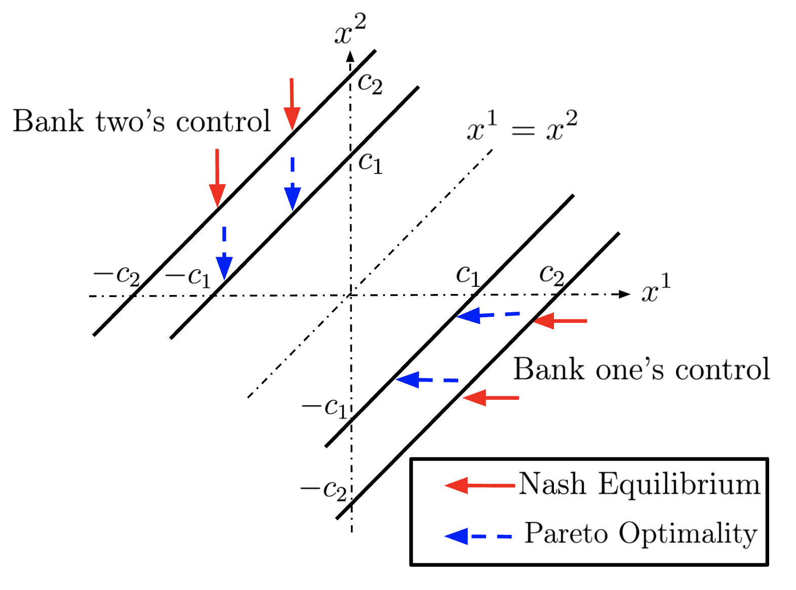
Figure 1: Comparison: Nash and Pareto ($K_{1}=K_{2}$).

Proof.

Similar to the derivation in (Guo  Xu, 2019), we have the following quasi-variational inequalities for the Nash equilibrium of game (5.1) with $J^{1}$ and $J^{2}$ and $K_{1}=K_{2}=K$,

$$\begin{cases}&\max\left\{\rho v^{i}(x^{1},x^{2})-h(x^{1}-x^{2})-\frac{\widetilde{\sigma}^{2}}{2}\Big{(}\partial^{2}_{x^{1}}v^{i}(x^{1},x^{2})+\partial^{2}_{x^{2}}v^{i}(x^{1},x^{2})\Big{)},\right.\\ &\hskip 150.0pt\partial_{x^{i}}v^{i}(x^{1},x^{2})-K,-\partial_{x^{i}}v^{i}(x^{1},x^{2})-K\Big{\}}=0,\\ &\hskip 210.0pt\mbox{on}\hskip 10.0pt\left\{(x^{1},x^{2}):-K<\partial_{x^{j}}v^{j}(x^{1},x^{2})<K\right\},\\ &\partial_{x^{i}}v^{i}(x^{1},x^{2})=0,\hskip 120.0pt\mbox{on}\hskip 10.0pt\left\{(x^{1},x^{2}):\partial_{x^{j}}v^{j}(x^{1},x^{2})=K\text{ or }\partial_{x^{j}}v^{j}(x^{1},x^{2})=-K\right\},\end{cases}$$

for $i\neq j$ and $1\leq i,j\leq 2$. Moreover, one can show that (5.34)-(5.38) are the solution to (5.2). Applying a verification theorem (Guo  Xu, 2019, Theorem 3), some further calculations can verify that (5.34)-(5.38) are the game values associated with the Nash equilibrium policy (5.29).

Now we provide the proof for Claim (ii). Define $g(x)=\frac{\widetilde{\sigma}}{\sqrt{2\rho}}\tanh\left(\frac{\sqrt{2\rho}}{\widetilde{\sigma}}x\right)$, $g_{1}(x)=\frac{p_{1}^{\prime}(x)-\frac{K}{2}}{p_{1}^{\prime\prime}(x)}$ and $g_{2}(x)=\frac{p_{1}^{\prime}(x)-K}{p_{1}^{\prime\prime}(x)}$, where $p_{1}$ is defined in (5.10). Then $g(0)=0$, $g^{\prime}(x)>0$ $\textit{ for any }x\in\mathbb{R^{+}}$, and $lim_{x\rightarrow\infty}g(x)=\frac{\widetilde{\sigma}}{\sqrt{2\rho}}$. Thanks to Assumption $({\bf B2})$,

$$0<\frac{c}{\rho}\leq p_{1}^{\prime\prime}(x)=\mathbb{E}\int_{0}^{\infty}e^{-\rho t}h^{\prime\prime}({x}+\widetilde{\sigma}B_{t})dt\leq\frac{C}{\rho}.$$

The function $p^{\prime}_{1}(x)$ is negative at $x=0$ and increases monotonically to $\infty$ on $\mathbb{R}^{+}$. Hence there exists an unique positive zero ${c}_{0}$. Moreover, for any $x>{c}_{0}$, $g_{1}^{\prime}(x)=1-\frac{p^{\prime\prime\prime}_{1}(x)}{p^{\prime\prime}_{1}(x)}g_{1}(x)\geq 1$. This is because $p^{\prime\prime\prime}_{1}(x)\leq 0$ for $x\geq 0$. We conclude that there exists a unique point ${c}_{0}<c_{1}<\infty$ such that $g(c_{1})=g_{1}(c_{1})$.

Now by similar analysis, $c_{2}$ is the unique solution to $g(x)=g_{2}(x)$ such that $0<c_{2}<\infty$. Notice that, $g_{1}(x)-g_{2}(x)=\frac{K}{2p_{1}^{\prime\prime}(x)}>0$ because $p_{2}^{\prime\prime}(x)>0$. Hence $c_{2}>c_{1}$. ∎

Appendix A Verification theorem

Theorem 21.

Let $u\in W_{\rm loc}^{2,\infty}(\mathbb{R}^{N})$ be a convex solution to the HJB equation (3.3) and $0\leq\partial^{2}_{\boldsymbol{\nu}}u(\boldsymbol{x})\leq C$ (in the weak sense). Under Assumptions A1-A3, $u$ is equal to the value function $v$ of (3):

$$v(\boldsymbol{x})=\min_{\boldsymbol{\xi}\in\mathcal{U}}J(\boldsymbol{x};\boldsymbol{\xi})=u(\boldsymbol{x}).$$

In addition, if there exists $\boldsymbol{\xi}^{*}\in\mathcal{U}$ such that

• $\boldsymbol{X}_{t}^{*}=\boldsymbol{x}+\boldsymbol{\sigma}\boldsymbol{B}_{t}+\boldsymbol{\xi}^{*}_{t}\in\overline{\mathcal{C}}_{N}$ for every $t\geq 0$, $\mathbb{P}$-a.s.;

• $\boldsymbol{\xi}^{*}_{t}=\boldsymbol{\xi}_{0}^{*}+\int_{0}^{t}\boldsymbol{N}_{s}d\eta^{*}_{s}$ with $\boldsymbol{\xi}_{0}^{*}=\pi(\boldsymbol{x})-\boldsymbol{x}$ and $\eta_{t}^{*}=\int_{0}^{t}{\bf 1}_{\{\boldsymbol{X}_{s}^{*}\in\partial\mathcal{C}_{N},\boldsymbol{N}_{s}\in\bf{r}(\boldsymbol{X}_{s}^{*})\}}d\eta^{*}_{s}$ for every $t\geq 0$, $\mathbb{P}$-a.s.;

• $\boldsymbol{\xi}^{*}$ is continuous if $\boldsymbol{\xi}_{0}^{*}=0$;

where $\mathcal{C}_{N}=\left\{\boldsymbol{x}\>\lvert\>\beta(\nabla u(\boldsymbol{x}))<1\right\}$, and $\gamma$ and $\boldsymbol{r}$ are defined in (4.5)-(4.6) such that Assumption A5 holds, then $\boldsymbol{\xi}^{*}$ is an optimal control.

Proof.

By the Sobolev embedding (Brezis, 2010, Ch. 9, Cor. 9.15), $u\in\mathcal{C}^{1}(\mathbb{R}^{N})$ since $u\in\mathcal{W}_{\rm loc}^{2,\infty}(\mathbb{R}^{N})$. In addition, $u$ is convex and $0\leq\partial^{2}_{\boldsymbol{\nu}}u(\boldsymbol{x})\leq C$, then apply the Itô-Tanaka-Meyer formula (Carlen  Protter, 1992) to the function $e^{-\rho t}u(\boldsymbol{X}_{t})$ of the semi-martingale $\boldsymbol{X}_{t}=\boldsymbol{x}+\boldsymbol{\mu}t+\boldsymbol{\sigma}\boldsymbol{B}_{t}+\boldsymbol{\xi}_{t}$,

$$e^{-\alpha T}u(\boldsymbol{X}_{t})-u(\boldsymbol{x}) = \int_{0}^{T}e^{-\alpha t}\nabla u(\boldsymbol{X}_{t})d\boldsymbol{B}_{t}+\int_{0}^{T}e^{-\alpha t}(\mathcal{L}u(\boldsymbol{X}_{t})-\alpha u(\boldsymbol{X}_{t}))dt$$ (A.1)

$$+\int_{0}^{T}e^{-\alpha T}(\sum_{i=1}^{N}\partial_{x^{i}}u(\boldsymbol{X}_{t})d\xi_{t}^{i,+}-\sum_{i=1}^{N}\partial_{x^{i}}u(\boldsymbol{X}_{t})d\xi_{t}^{i,-})$$

$$+\sum_{0\leq t\leq T}e^{-\alpha T}\left(\Delta u(\boldsymbol{X}_{t})-\sum_{i=1}^{N}\partial_{x^{i}}u(\boldsymbol{X}_{t})\Delta X_{t}^{i}\right),$$

with the notation $\Delta\phi_{t}:=\phi_{t}-\phi_{t-}$. Since $u$ is a convex solution to the HJB equation (3.3), we have $\mathbb{P}$-a.s. for all $0\leq t\leq T$,

$$\rho u(\boldsymbol{X}_{t})-\mathcal{L}u(\boldsymbol{X}_{t})-H((\boldsymbol{X}_{t}))\leq 0,$$ (A.2)

$$\partial_{x^{i}}u(\boldsymbol{X}_{t})d\xi_{t}^{i,-}\leq L_{i}K_{i}^{-}d\xi_{t}^{i,-},-L_{i}K_{i}^{+}d\xi_{t}^{i,+}\leq\partial_{x^{i}}u(\boldsymbol{X}_{t})d\xi_{t}^{i,+},$$ (A.3)

$$\Delta u(\boldsymbol{X}_{t})-\sum_{i=1}^{N}\partial_{x^{i}}u(\boldsymbol{X}_{t})\Delta X_{t}^{i}\geq 0.$$ (A.4)

Taking expectation on both sides of (A.1), we have for any admissible policy $\boldsymbol{\xi}$,

$$e^{-\alpha T}\mathbb{E}[u(\boldsymbol{X}_{t})]+\mathbb{E}\int_{0}^{T}e^{-\rho t}\Big{(}H(\boldsymbol{X}_{t})dt+K_{i}^{+}d\xi_{t}^{i,+}+K_{i}^{-}d\xi_{t}^{i,-}\Big{)}\geq u(\boldsymbol{x}).$$ (A.5)

Since $0\leq\partial^{2}_{\boldsymbol{\nu}}u(\boldsymbol{x})\leq C$, there exists constant $K=K(C)>0$ such that $|u(\boldsymbol{x})|\leq K(1+\|\boldsymbol{x}\|^{2})$. Hence $\mathbb{E}[u(\boldsymbol{X}_{t})]\leq 9K\left(1+\|\boldsymbol{x}\|^{2}+\|\boldsymbol{\sigma}\|^{2}\|\boldsymbol{B}_{T}\|^{2}+\|\boldsymbol{\xi}_{T}\|^{2}\right)$.

Now we show that $\mathbb{E}[\|\boldsymbol{\xi}_{T}\|^{2}]=o(e^{\rho t})$. If this does not hold, then standard arguments (e.g. (Widder, 1941, P 39)) can show that there exists $i\in\{1,2,\cdots,N\}$ such that $\mathbb{E}[\int_{0}^{\infty}e^{-\rho t}(d\xi_{t}^{i,+}+d\xi_{t}^{i,-})]=\infty$, which violates the condition in the definition of admissible control set $\mathcal{U}_{N}$. Hence by letting $T\rightarrow\infty$ we have

$$\mathbb{E}\int_{0}^{\infty}e^{-\rho t}\Big{(}H(\boldsymbol{X}_{t})dt+K_{i}^{+}d\xi_{t}^{i,+}+K_{i}^{-}d\xi_{t}^{i,-}\Big{)}\geq u(\boldsymbol{x}).$$ (A.6)

Under Assumption A1-A3, Theorem 5 holds and hence $u(\boldsymbol{x})=v(\boldsymbol{x})$ for all $\boldsymbol{x}\in\mathbb{R}^{N}$.

To achieve the equality in (A.6), it suffices to achieve the equalities in conditions (A.2)-(A.4), which requires the following properties from the optimal control process $\boldsymbol{\xi}^{*}$:

• $\boldsymbol{X}_{t}^{*}=\boldsymbol{x}+\boldsymbol{\sigma}\boldsymbol{B}_{t}+\boldsymbol{\xi}^{*}_{t}\in\overline{\mathcal{C}}_{N}$ hence $\rho u(\boldsymbol{X}^{*}_{t})-\mathcal{L}u(\boldsymbol{X}^{*}_{t})-H(\boldsymbol{X}^{*}_{t})=0$ for every $t\geq 0$, $\mathbb{P}$-a.s.;

• The only possible jump is at time $0$ when $\boldsymbol{x}\notin\mathcal{C}_{N}$. Under Assumption A5 and the convexity of $u$, we can show that $u(\boldsymbol{x})=u(\pi(\boldsymbol{x}))+l(\boldsymbol{x}-\pi(\boldsymbol{x}))$ with $l(\boldsymbol{y})=\sum_{i}l_{i}(y_{i})$, where

  $$l_{i}(y_{i})=\left\{\begin{array}[]{ll}L_{i}K_{i}^{-}y_{i},\quad\mbox{ if }y_{i}\geq 0,\\ -L_{i}K^{+}_{i}y_{i},\quad\mbox{ if }y_{i}<0.\end{array}\right.$$ (A.9)

  The proof is the same as the one for Theorem 11. And hence the equality in (A.4) holds.

• By the definition of $\boldsymbol{\xi}^{*}$, $d\boldsymbol{\xi}_{t}^{*}\neq 0$ only when $\boldsymbol{X}^{*}_{t-}\notin\mathcal{C}_{N}$. Hence the equality in (A.3) holds.

∎

References

- Aïd \BOthers. (\APACyear2017) \APACinsertmetastarABP2017{APACrefauthors}Aïd, R., Basei, M.\BCBL \BBA Pham, H. \APACrefYearMonthDay2017. \BBOQ\APACrefatitleThe coordination of centralised and distributed generation The coordination of centralised and distributed generation.\BBCQ \APACjournalVolNumPagesarXiv preprint arXiv:1705.01302. \PrintBackRefs\CurrentBib
- Avellaneda \BBA Cont (\APACyear2010) \APACinsertmetastaravellaneda2010{APACrefauthors}Avellaneda, M.\BCBT \BBA Cont, R. \APACrefYearMonthDay2010. \APACrefbtitleTransparency in over-the-counter interest rate derivatives markets Transparency in over-the-counter interest rate derivatives markets \APACbVolEdTRReport. \APACaddressInstitutionFinance Concepts. \PrintBackRefs\CurrentBib
- Bator (\APACyear1957) \APACinsertmetastarBator1957{APACrefauthors}Bator, F\BPBIM. \APACrefYearMonthDay1957. \BBOQ\APACrefatitleThe simple analytics of welfare maximization The simple analytics of welfare maximization.\BBCQ \APACjournalVolNumPagesThe American Economic Review47122–59. \PrintBackRefs\CurrentBib
- Beneš \BOthers. (\APACyear1980) \APACinsertmetastarBSW1980{APACrefauthors}Beneš, V\BPBIE., Shepp, L\BPBIA.\BCBL \BBA Witsenhausen, H\BPBIS. \APACrefYearMonthDay1980. \BBOQ\APACrefatitleSome solvable stochastic control problems Some solvable stochastic control problems.\BBCQ \APACjournalVolNumPagesStochastics: An International Journal of Probability and Stochastic Processes4139–83. \PrintBackRefs\CurrentBib
- Bensoussan \BOthers. (\APACyear2012) \APACinsertmetastarbensoussan2012{APACrefauthors}Bensoussan, A., Long, H., Perera, S.\BCBL \BBA Sethi, S. \APACrefYearMonthDay2012. \BBOQ\APACrefatitleImpulse control with random reaction periods: a central bank intervention problem Impulse control with random reaction periods: a central bank intervention problem.\BBCQ \APACjournalVolNumPagesOperations Research Letters406425–430. \PrintBackRefs\CurrentBib
- Brezis (\APACyear2010) \APACinsertmetastarbrezis2010functional{APACrefauthors}Brezis, H. \APACrefYear2010. \APACrefbtitleFunctional Analysis, Sobolev Spaces and Partial Differential Equations Functional Analysis, Sobolev Spaces and Partial Differential Equations. \APACaddressPublisherSpringer. \PrintBackRefs\CurrentBib
- Cadenillas \BBA Zapatero (\APACyear2000) \APACinsertmetastarcadenillas2000{APACrefauthors}Cadenillas, A.\BCBT \BBA Zapatero, F. \APACrefYearMonthDay2000. \BBOQ\APACrefatitleClassical and impulse stochastic control of the exchange rate using interest rates and reserves Classical and impulse stochastic control of the exchange rate using interest rates and reserves.\BBCQ \APACjournalVolNumPagesMathematical Finance102141–156. \PrintBackRefs\CurrentBib
- Carlen \BBA Protter (\APACyear1992) \APACinsertmetastarcarlen1992semimartingale{APACrefauthors}Carlen, E.\BCBT \BBA Protter, P. \APACrefYearMonthDay1992. \BBOQ\APACrefatitleOn semimartingale decompositions of convex functions of semimartingales On semimartingale decompositions of convex functions of semimartingales.\BBCQ \APACjournalVolNumPagesIllinois journal of mathematics363420–427. \PrintBackRefs\CurrentBib
- Carmona \BOthers. (\APACyear2015) \APACinsertmetastarCFS2013{APACrefauthors}Carmona, R., Fouque, J\BHBIP.\BCBL \BBA Sun, L\BHBIH. \APACrefYearMonthDay2015. \BBOQ\APACrefatitleMean field games and systemic risk Mean field games and systemic risk.\BBCQ \APACjournalVolNumPagesCommunications in Mathematical Sciences134911–933. \PrintBackRefs\CurrentBib
- Chiarolla \BOthers. (\APACyear2013) \APACinsertmetastarCFR2013{APACrefauthors}Chiarolla, M\BPBIB., Ferrari, G.\BCBL \BBA Riedel, F. \APACrefYearMonthDay2013. \BBOQ\APACrefatitleGeneralized Kuhn–Tucker Conditions for N-Firm Stochastic Irreversible Investment under Limited Resources Generalized Kuhn–Tucker conditions for N-firm stochastic irreversible investment under limited resources.\BBCQ \APACjournalVolNumPagesSIAM Journal on Control and Optimization5153863–3885. \PrintBackRefs\CurrentBib
- Coleman (\APACyear1979) \APACinsertmetastarColeman1979{APACrefauthors}Coleman, J\BPBIL. \APACrefYearMonthDay1979. \BBOQ\APACrefatitleEfficiency, utility, and wealth maximization Efficiency, utility, and wealth maximization.\BBCQ \APACjournalVolNumPagesHofstra L. Rev.8509. \PrintBackRefs\CurrentBib
- Davis \BBA Norman (\APACyear1990) \APACinsertmetastardavis1990portfolio{APACrefauthors}Davis, M\BPBIH.\BCBT \BBA Norman, A\BPBIR. \APACrefYearMonthDay1990. \BBOQ\APACrefatitlePortfolio selection with transaction costs Portfolio selection with transaction costs.\BBCQ \APACjournalVolNumPagesMathematics of Operations Research154676–713. \PrintBackRefs\CurrentBib
- Davis \BOthers. (\APACyear1993) \APACinsertmetastardavis1993european{APACrefauthors}Davis, M\BPBIH., Panas, V\BPBIG.\BCBL \BBA Zariphopoulou, T. \APACrefYearMonthDay1993. \BBOQ\APACrefatitleEuropean option pricing with transaction costs European option pricing with transaction costs.\BBCQ \APACjournalVolNumPagesSIAM Journal on Control and Optimization312470–493. \PrintBackRefs\CurrentBib
- De Angelis \BBA Ferrari (\APACyear2018) \APACinsertmetastarDF2018{APACrefauthors}De Angelis, T.\BCBT \BBA Ferrari, G. \APACrefYearMonthDay2018. \BBOQ\APACrefatitleStochastic nonzero-sum games: a new connection between singular control and optimal stopping Stochastic nonzero-sum games: a new connection between singular control and optimal stopping.\BBCQ \APACjournalVolNumPagesAdvances in Applied Probability502347–372. \PrintBackRefs\CurrentBib
- Dianetti \BBA Ferrari (\APACyear2020) \APACinsertmetastardianetti2020nonzero{APACrefauthors}Dianetti, J.\BCBT \BBA Ferrari, G. \APACrefYearMonthDay2020. \BBOQ\APACrefatitleNonzero-Sum Submodular Monotone-Follower Games: existence and Approximation of Nash Equilibria Nonzero-sum submodular monotone-follower games: existence and approximation of Nash equilibria.\BBCQ \APACjournalVolNumPagesSIAM Journal on Control and Optimization5831257–1288. \PrintBackRefs\CurrentBib
- Duffie \BBA Stein (\APACyear2015) \APACinsertmetastarduffie2015{APACrefauthors}Duffie, D.\BCBT \BBA Stein, J\BPBIC. \APACrefYearMonthDay2015. \BBOQ\APACrefatitleReforming LIBOR and other financial market benchmarks Reforming LIBOR and other financial market benchmarks.\BBCQ \APACjournalVolNumPagesJournal of Economic Perspectives292191–212. \PrintBackRefs\CurrentBib
- Dupuis \BBA Ishii (\APACyear1991) \APACinsertmetastarDI1991{APACrefauthors}Dupuis, P.\BCBT \BBA Ishii, H. \APACrefYearMonthDay1991. \BBOQ\APACrefatitleOn Lipschitz continuity of the solution mapping to the Skorokhod problem, with applications On Lipschitz continuity of the solution mapping to the Skorokhod problem, with applications.\BBCQ \APACjournalVolNumPagesStochastics35131–62. \PrintBackRefs\CurrentBib
- Dupuis \BBA Ishii (\APACyear1993) \APACinsertmetastarDI1993{APACrefauthors}Dupuis, P.\BCBT \BBA Ishii, H. \APACrefYearMonthDay1993. \BBOQ\APACrefatitleSDEs with Oblique Reflection on Nonsmooth Domains SDEs with Oblique Reflection on Nonsmooth Domains.\BBCQ \APACjournalVolNumPagesAnnals of Probability211554 – 580. {APACrefDOI} \doi10.1214/aop/1176989415 \PrintBackRefs\CurrentBib
- Evans (\APACyear1990) \APACinsertmetastarevans1990weak{APACrefauthors}Evans, L\BPBIC. \APACrefYear1990. \APACrefbtitleWeak Convergence Methods for Nonlinear Partial Differential Equations Weak convergence methods for nonlinear partial differential equations. \APACaddressPublisherAmerican Mathematical Society. \PrintBackRefs\CurrentBib
- Ferrari \BOthers. (\APACyear2017) \APACinsertmetastarFRS2017{APACrefauthors}Ferrari, G., Riedel, F.\BCBL \BBA Steg, J\BHBIH. \APACrefYearMonthDay2017. \BBOQ\APACrefatitleContinuous-time public good contribution under uncertainty: a stochastic control approach Continuous-time public good contribution under uncertainty: a stochastic control approach.\BBCQ \APACjournalVolNumPagesApplied Mathematics & Optimization753429–470. \PrintBackRefs\CurrentBib
- Fischer \BBA Livieri (\APACyear2016) \APACinsertmetastarFL2016{APACrefauthors}Fischer, M.\BCBT \BBA Livieri, G. \APACrefYearMonthDay2016. \BBOQ\APACrefatitleContinuous time mean-variance portfolio optimization through the mean field approach Continuous time mean-variance portfolio optimization through the mean field approach.\BBCQ \APACjournalVolNumPagesESAIM: Probability and Statistics2030–44. \PrintBackRefs\CurrentBib
- Gilbarg \BBA Trudinger (\APACyear2015) \APACinsertmetastarGT2015{APACrefauthors}Gilbarg, D.\BCBT \BBA Trudinger, N\BPBIS. \APACrefYear2015. \APACrefbtitleElliptic Partial Differential Equations of Second Order Elliptic Partial Differential Equations of Second Order. \APACaddressPublisherSpringer. \PrintBackRefs\CurrentBib
- Gomes \BOthers. (\APACyear2010) \APACinsertmetastarGMS2010{APACrefauthors}Gomes, D\BPBIA., Mohr, J.\BCBL \BBA Souza, R\BPBIR. \APACrefYearMonthDay2010. \BBOQ\APACrefatitleDiscrete time, finite state space mean field games Discrete time, finite state space mean field games.\BBCQ \APACjournalVolNumPagesJournal de Mathématiques Pures et Appliquées933308–328. \PrintBackRefs\CurrentBib
- Guo \BBA Pham (\APACyear2005) \APACinsertmetastarGP2005{APACrefauthors}Guo, X.\BCBT \BBA Pham, H. \APACrefYearMonthDay2005. \BBOQ\APACrefatitleOptimal partially reversible investment with entry decision and general production function Optimal partially reversible investment with entry decision and general production function.\BBCQ \APACjournalVolNumPagesStochastic Processes and their Applications1155705–736. \PrintBackRefs\CurrentBib
- Guo \BBA Xu (\APACyear2019) \APACinsertmetastarGX2019{APACrefauthors}Guo, X.\BCBT \BBA Xu, R. \APACrefYearMonthDay2019. \BBOQ\APACrefatitleStochastic Games for Fuel Follower Problem: N versus MFG Stochastic games for fuel follower problem: N versus MFG.\BBCQ \APACjournalVolNumPagesSIAM Journal on Control and Optimization571659–692. \PrintBackRefs\CurrentBib
- H. M. Treasury (\APACyear2012) \APACinsertmetastarwheatley{APACrefauthors}H. M. Treasury. \APACrefYearMonthDay2012. \APACrefbtitleThe Wheatley Review of LIBOR: Final Report The Wheatley Review of LIBOR: Final Report \APACbVolEdTR\BTR. \APACaddressInstitutionEqAuthH. M. Treasury. {APACrefURL} https://assets.publishing.service.gov.uk/government/uploads/system/uploads/attachment_data/file/191762/wheatley_review_libor_finalreport_280912.pdf \PrintBackRefs\CurrentBib
- Hernandez-Hernandez \BOthers. (\APACyear2015) \APACinsertmetastarhernandez2015zero{APACrefauthors}Hernandez-Hernandez, D., Simon, R\BPBIS.\BCBL \BBA Zervos, M. \APACrefYearMonthDay2015. \BBOQ\APACrefatitleA zero-sum game between a singular stochastic controller and a discretionary stopper A zero-sum game between a singular stochastic controller and a discretionary stopper.\BBCQ \APACjournalVolNumPagesAnnals of Applied Probability25146–80. \PrintBackRefs\CurrentBib
- Huang \BOthers. (\APACyear2006) \APACinsertmetastarHMC2006{APACrefauthors}Huang, M., Malhamé, R\BPBIP.\BCBL \BBA Caines, P\BPBIE. \APACrefYearMonthDay2006. \BBOQ\APACrefatitleLarge population stochastic dynamic games: closed-loop McKean-Vlasov systems and the Nash certainty equivalence principle Large population stochastic dynamic games: closed-loop McKean-Vlasov systems and the Nash certainty equivalence principle.\BBCQ \APACjournalVolNumPagesCommunications in Information & Systems63221–252. \PrintBackRefs\CurrentBib
- Jeanblanc-Picqué (\APACyear1993) \APACinsertmetastarjeanblanc1993impulse{APACrefauthors}Jeanblanc-Picqué, M. \APACrefYearMonthDay1993. \BBOQ\APACrefatitleImpulse control method and exchange rate Impulse control method and exchange rate.\BBCQ \APACjournalVolNumPagesMathematical Finance32161–177. \PrintBackRefs\CurrentBib
- Kallsen \BBA Muhle-Karbe (\APACyear2017) \APACinsertmetastarkallsen2017general{APACrefauthors}Kallsen, J.\BCBT \BBA Muhle-Karbe, J. \APACrefYearMonthDay2017. \BBOQ\APACrefatitleThe general structure of optimal investment and consumption with small transaction costs The general structure of optimal investment and consumption with small transaction costs.\BBCQ \APACjournalVolNumPagesMathematical Finance273659–703. \PrintBackRefs\CurrentBib
- Karatzas (\APACyear1983) \APACinsertmetastarkaratzas1982{APACrefauthors}Karatzas, I. \APACrefYearMonthDay1983. \BBOQ\APACrefatitleA class of singular stochastic control problems A class of singular stochastic control problems.\BBCQ \APACjournalVolNumPagesAdvances in Applied Probability152225 – 254. \PrintBackRefs\CurrentBib
- Kruk (\APACyear2000) \APACinsertmetastarkruk2000{APACrefauthors}Kruk, L. \APACrefYearMonthDay2000. \BBOQ\APACrefatitleOptimal policies for N-dimensional singular stochastic control problems part I: the Skorokhod problem Optimal policies for N-dimensional singular stochastic control problems part I: the Skorokhod problem.\BBCQ \APACjournalVolNumPagesSIAM Journal on Control and Optimization3851603–1622. \PrintBackRefs\CurrentBib
- Kwon \BBA Zhang (\APACyear2015) \APACinsertmetastarKZ2015{APACrefauthors}Kwon, H.\BCBT \BBA Zhang, H. \APACrefYearMonthDay2015. \BBOQ\APACrefatitleGame of singular stochastic control and strategic exit Game of singular stochastic control and strategic exit.\BBCQ \APACjournalVolNumPagesMathematics of Operations Research404869–887. \PrintBackRefs\CurrentBib
- Lasry \BBA Lions (\APACyear2007) \APACinsertmetastarLL2007{APACrefauthors}Lasry, J\BHBIM.\BCBT \BBA Lions, P\BHBIL. \APACrefYearMonthDay2007. \BBOQ\APACrefatitleMean field games Mean field games.\BBCQ \APACjournalVolNumPagesJapanese Journal of Mathematics21229–260. \PrintBackRefs\CurrentBib
- Menaldi \BBA Robin (\APACyear1983) \APACinsertmetastarMR1983{APACrefauthors}Menaldi, J\BHBIL.\BCBT \BBA Robin, M. \APACrefYearMonthDay1983. \BBOQ\APACrefatitleOn some cheap control problems for diffusion processes On some cheap control problems for diffusion processes.\BBCQ \APACjournalVolNumPagesTransactions of the American Mathematical Society2782771–802. \PrintBackRefs\CurrentBib
- Menaldi \BBA Taksar (\APACyear1989) \APACinsertmetastarMT1989{APACrefauthors}Menaldi, J\BHBIL.\BCBT \BBA Taksar, M\BPBII. \APACrefYearMonthDay1989. \BBOQ\APACrefatitleOptimal correction problem of a multidimensional stochastic system Optimal correction problem of a multidimensional stochastic system.\BBCQ \APACjournalVolNumPagesAutomatica252223–232. \PrintBackRefs\CurrentBib
- Meyer (\APACyear1976) \APACinsertmetastarMeyer76{APACrefauthors}Meyer, P\BPBIA. \APACrefYearMonthDay1976. \BBOQ\APACrefatitleMartingales locales changement de variables, formules exponentielles Martingales locales changement de variables, formules exponentielles.\BBCQ \BIn \APACrefbtitleSéminaire de Probabilités X Université de Strasbourg Séminaire de Probabilités X Université de Strasbourg (\BPGS 291–331). \APACaddressPublisherSpringer. \PrintBackRefs\CurrentBib
- Ramanan (\APACyear2006) \APACinsertmetastarramanan2006{APACrefauthors}Ramanan, K. \APACrefYearMonthDay2006. \BBOQ\APACrefatitleReflected diffusions defined via the extended Skorokhod map Reflected diffusions defined via the extended Skorokhod map.\BBCQ \APACjournalVolNumPagesElectronic journal of probability11934–992. \PrintBackRefs\CurrentBib
- Rosen (\APACyear1987) \APACinsertmetastarrosen1987{APACrefauthors}Rosen, J. \APACrefYearMonthDay1987. \BBOQ\APACrefatitleJoint continuity of the intersection local times of Markov processes Joint continuity of the intersection local times of Markov processes.\BBCQ \APACjournalVolNumPagesAnnals of Probability15659–675. \PrintBackRefs\CurrentBib
- Soner \BBA Shreve (\APACyear1989) \APACinsertmetastarSS1989{APACrefauthors}Soner, H\BPBIM.\BCBT \BBA Shreve, S\BPBIE. \APACrefYearMonthDay1989. \BBOQ\APACrefatitleRegularity of the value function for a two-dimensional singular stochastic control problem Regularity of the value function for a two-dimensional singular stochastic control problem.\BBCQ \APACjournalVolNumPagesSIAM Journal on Control and Optimization274876–907. \PrintBackRefs\CurrentBib
- Sun (\APACyear2018) \APACinsertmetastarsun2018{APACrefauthors}Sun, L\BHBIH. \APACrefYearMonthDay2018. \BBOQ\APACrefatitleSystemic risk and interbank lending Systemic risk and interbank lending.\BBCQ \APACjournalVolNumPagesJournal of Optimization Theory and Applications1792400–424. \PrintBackRefs\CurrentBib
- Wang \BBA Ewald (\APACyear2010) \APACinsertmetastarWE2010{APACrefauthors}Wang, W\BHBIK.\BCBT \BBA Ewald, C\BHBIO. \APACrefYearMonthDay2010. \BBOQ\APACrefatitleDynamic voluntary provision of public goods with uncertainty: a stochastic differential game model Dynamic voluntary provision of public goods with uncertainty: a stochastic differential game model.\BBCQ \APACjournalVolNumPagesDecisions in Economics and Finance33297–116. \PrintBackRefs\CurrentBib
- Widder (\APACyear1941) \APACinsertmetastarwidder2015laplace{APACrefauthors}Widder, D\BPBIV. \APACrefYear1941. \APACrefbtitleThe Laplace Transform The Laplace Transform. \APACaddressPublisherPrinceton university press. \PrintBackRefs\CurrentBib
- Williams \BOthers. (\APACyear1994) \APACinsertmetastarWCM1994{APACrefauthors}Williams, S., Chow, P.\BCBL \BBA Menaldi, J. \APACrefYearMonthDay1994. \BBOQ\APACrefatitleRegularity of the Free Boundary in Singular Stochastic Control Regularity of the free boundary in singular stochastic control.\BBCQ \APACjournalVolNumPagesJournal of Differential Equations1111175 - 201. \PrintBackRefs\CurrentBib
- Zariphopoulou (\APACyear1992) \APACinsertmetastarzariphopoulou1992investment{APACrefauthors}Zariphopoulou, T. \APACrefYearMonthDay1992. \BBOQ\APACrefatitleInvestment-consumption models with transaction fees and Markov-chain parameters Investment-consumption models with transaction fees and Markov-chain parameters.\BBCQ \APACjournalVolNumPagesSIAM Journal on Control and Optimization303613–636. \PrintBackRefs\CurrentBib