CSB-RNN: A Faster-than-Realtime RNN Acceleration Framework with Compressed Structured Blocks

Abstract.

Recurrent neural networks (RNNs) have been widely adopted in temporal sequence analysis, where realtime performance is often in demand. However, RNNs suffer from heavy computational workload as the model often comes with large weight matrices. Pruning (a model compression method) schemes have been proposed for RNNs to eliminate the redundant (close-to-zero) weight values. On one hand, the non-structured pruning methods achieve a high pruning rate but introducing computation irregularity (random sparsity), which is unfriendly to parallel hardware. On the other hand, hardware-oriented structured pruning suffers from low pruning rate due to restricted constraints on allowable pruning structure.

This paper presents CSB-RNN, an optimized full-stack RNN framework with a novel compressed structured block (CSB) pruning technique. The CSB pruned RNN model comes with both fine pruning granularity that facilitates a high pruning rate and regular structure that benefits the hardware parallelism. To address the challenges in parallelizing the CSB pruned model inference with fine-grained structural sparsity, we propose a novel hardware architecture with a dedicated compiler. Gaining from the architecture-compilation co-design, the hardware not only supports various RNN cell types, but is also able to address the challenging workload imbalance issue and therefore significantly improves the hardware efficiency (utilization). Compared to the vanilla design without optimizations, the hardware utilization has been enhanced by over $2\times$. With experiments on $10$ RNN models from multiple application domains, CSB pruning demonstrates $3.5\times$-$25\times$ lossless pruning rate, which is $1.6\times$ to $3.9\times$ over existing designs. With several other innovations applied, the CSB-RNN inference can achieve faster-than-realtime latency of $0.79\mu$s-$6.58\mu$s in an FPGA implementation, which contributes to $1.12\times$-$12.57\times$ lower latency and $3.53\times$-$58.89\times$ improvement on power-efficiency over the state-of-the-art.

1. Introduction

RNNs have been widely adopted for its high-accuracy on temporal sequence analysis, such as machine translation (Cho et al., 2014), speech recognition (Graves et al., 2013), or even stock-price prediction (Selvin et al., 2017). However, the increasingly large model size and tremendous computational workload of the RNN hampers its deployment on embedded (edge) devices, which strictly demand realtime processing with limited hardware resources. To address this issue, weight pruning techniques (Lym et al., 2019; Han et al., 2015; Wen et al., 2018) have been proposed, which shrink the model size, reduce storage demand, and provide higher potential hardware performance by eliminating the redundant (close-to-zero) weights and the corresponding arithmetic operations in inference.

The weight pruning schemes in some existing works (Han et al., 2015; Shi et al., 2019) are in a non-structured fashion and with extreme irregularities in the computation, which is unfriendly to either the modern parallel device or the hardware architecture design. Thus the performance degradation from the hardware inefficiency encroaches upon the gains from model compression. Therefore, researchers start to explore other pruning approaches, i.e., structured pruning (Wen et al., 2018; Mao et al., 2017; Narang et al., 2017), in which the regular computation patterns are maintained. Although these structured-pruned models are relatively hardware-friendly, the coarse pruning granularity (structure) leads to either a significant degradation on model accuracy or a limited pruning rate (the weight count ratio of the original model to pruned model). To keep the accuracy loss acceptable, the attainable pruning rates delivered in the existing structured pruning schemes are far lower than that the ones with the non-structured pruning, wasting potential pruning opportunities.

In this paper, we aim to overcome the above limitations. We first propose a novel fine-grained structured pruning technique (CSB pruning) that provides a similar compression rate (and test accuracy) as non-structured pruning while offering a higher potential for hardware acceleration than the non-structured methods. During the training phase, each weight matrices are divided into fine-grained blocks, and a structured pruning is conducted on every block independently. The pruned blocks are encoded in a novel compressed structured block (CSB) sparse format for inference acceleration, which significantly reduces the weight storage demand while retaining the fine-grained content in the original model.

To realize a realtime inference with parallel hardware, there are still multiple challenges to design an architecture that can exploit the benefits of CSB pruning in a seamless manner. In particular, the parallel architecture should handle massive fine-grained blocks with imbalanced workloads (sparsity) but maintain a high hardware efficiency (utilization). Meanwhile, the architecture should be programmable for various RNN cell types (e.g., LSTM (Hochreiter and Schmidhuber, 1997), GRU (Cho et al., 2014)), although the existing RNN architectures are designed for a particular cell type. To address the issues above, we propose an architecture-compilation co-design to realize the best flexibility and acceleration performance. A programmable RNN dataflow architecture is designed that supports existing RNN cell types. In particular, the $\mathtt{CSB}$-$\mathtt{Engine}$ in our architecture is designed with a novel workload sharing technique. With the one-shot compilation, the workload is automatically balanced among processing elements (PEs) in $\mathtt{CSB}$-$\mathtt{Engine}$, which improves the hardware efficiency to a near theoretical value.

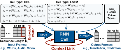
Figure 1. Computation flow of RNN inference. Note that there are multiple RNN cell types. The main workload is matrix-vector multiplication (MVM).

The major contributions are summarized as follows:

• We present CSB-RNN, an optimized full-stack RNN acceleration framework, which facilitates running various types of RNNs with faster-than-realtime latency. CSB-RNN includes three innovations: (1) an adaptive and fine-grained structured compression technique, CSB pruning; (2) a programmable RNN dataflow architecture equipped with $\mathtt{CSB}$-$\mathtt{Engine}$; (3) a compiler design with optimizations to achieve almost perfect workload balance.

• The proposed CSB pruning technique provides ultra-high ($3.5\times$-$25\times$) pruning rates without any loss on accuracy. Furthermore, CSB pruning does not incur high-degree computational irregularities, making highly efficient hardware acceleration possible.

• An architecture-compilation co-design is proposed to sufficiently exploit the benefits of CSB pruning and provide close-to-theoretical peak performance with automatic workload balancing.

• With experiments on $10$ RNN models from various application domains, CSB pruning demonstrates $3.5\times$-$25\times$ lossless pruning rate, which is $1.6\times$ to $3.9\times$ over existing designs. With the proposed architecture-compilation co-design applied, the CSB-RNN delivers faster-than-realtime inference with the latency of $0.79\mu$s-$6.58\mu$s in an FPGA implementation. The proposed framework contributes to $1.12\times$-$12.57\times$ lower latency (with even fewer computation resources) and $3.53\times$-$58.89\times$ improvement on power-efficiency over the state-of-the-art.

2. Background

2.1. Temporal Sequence Processing with RNN

The recurrent neural networks (RNNs) deliver high accuracy in the temporal sequence processing. A typical schematic of RNN computation is depicted in Fig. 1. Successive frames (e.g., word, phoneme) from the temporal sequence (e.g., sentence, voice) are embedded as input neuron-vectors ($x_{t}$), and then sent to RNN cells for inference computation. $t$ represents the time point. The output neuron-vector ($h_{t}$) contains the inference results (e.g., translation, prediction) that may have different dimensions with $x_{t}$.

Multiple RNN cell types exist that are composed of different computational dataflow but almost the same arithmetic primitives. Fig. 1 lists the arithmetic of two widely-used RNN cells, GRU (Cho et al., 2014) and LSTM (Hochreiter and Schmidhuber, 1997). The significant workload is matrix-vector multiplication (MVM) between the weight matrices and input/hidden neurons; And the rest workload is element-wise operations, including Sigmoid ($\sigma$)/Tanh ($\theta$) activation function, element-wise multiplication ($\odot$) and addition. In particular, the RNN cell computation at time $t$ invokes the intermediate vector $c_{t-1}$ and output vector $h_{t-1}$ from the previous timestamp. The data dependency results in a context link between two successive RNN cell iterations, which helps to memorize the temporal feature during inference.

2.2. RNN Weight Pruning Techniques

2.2.1. Non-structured Pruning v.s. Structured Pruning

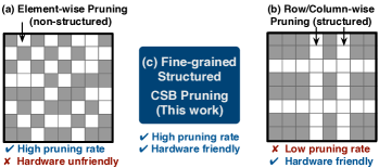
Figure 2. CSB pruning takes advantage of both non-structured (random) pruning (a) and coarse-grained structured (row/column) pruning (b).

The pruning technique has been proposed for deep learning models to reduce redundant (close-to-zero) weights and thus the computation workload. The early non-structured pruning (Han et al., 2015) achieves a high pruning rate; however, the random sparse model (Fig. 2(a)) brings a high degree of irregularity to the inference computation, which is unfriendly to either the modern parallel device or the hardware architecture design. Some existing works (Han et al., 2017; Cao et al., 2019) address this issue by pruning model with region-balanced sparsity (between non-structured and structured sparsity), which reduced the attainable pruning rate. As Fig. 2(b), the structured pruning schemes (Wen et al., 2016; Gao et al., 2018) were proposed for hardware friendly purpose that the entire row/column is removed as a whole in pruning. Although the pruned model maintains the regularity and can even be compacted to a dense matrix, the pruning rate with this scheme is relatively low due to the coarse pruning granularity. With the advantages of both the non-structured and coarse-grained structured pruning methods, the CSB pruning in this work is a fine-grained structured method that not only achieves a high pruning rate but also makes the hardware acceleration possible.

2.2.2. Model Training with ADMM-based Pruning Technique

The training process is to find a proper set of weight values that reach the minimal classification loss compared to the ground truth. The objective of training an $N$-layer RNN can be formulated as,

(1) $$\operatorname*{minimize}_{\{\mathbf{W}_{i}\},\{\mathbf{b}_{i}\}} f(\{\mathbf{W}_{i}\}_{i=1}^{N},\{\mathbf{b}_{i}\}_{i=1}^{N})$$

$$s.t. \mathbf{W}_{i}\in\mathbf{S}_{i},i=1,...,N$$

where function $f$ represents inference loss on the given dataset, $\mathbf{S}_{i}$ is the feasible set of $\mathbf{W}_{i}$, which is subject to the user constraints. In the regular RNN training, $\mathbf{S}_{i}$ is $\mathbb{R}$ (i.e., no constraint), and thus the optimal weights ($\mathbf{W}_{i}$) and bias ($\mathbf{b}_{i}$) for each layer can be obtained by classical stochastic gradient descent (SGD) method (Bottou, 2010). However, once the weight pruning is conducted along with the training process, the constraint of weight-sparsity represented by $\mathbf{S}_{i}$ becomes combinatorial and no longer convex, which prevents the Eqn. 1 from being solved by classical SGD. The advanced Alternating Direction Method of Multipliers (ADMM) method (Boyd et al., 2011) is leveraged in our CSB pruning scheme. The ADMM separates the weight pruning (during training) problem into two subproblems, which are iteratively solved until convergence. First, the problem is reformulated as,

(2) $$\operatorname*{minimize}_{\{\mathbf{W}_{i}\},\{\mathbf{b}_{i}\}} f(\{\mathbf{W}_{i}\}_{i=1}^{N},\{\mathbf{b}_{i}\}_{i=1}^{N})+\sum_{i=1}^{N}g_{i}(\mathbf{Z}_{i})$$

$$s.t. \mathbf{W}_{i}=\mathbf{Z}_{i},i=1,...,N$$

where $\mathbf{Z}_{i}$ is an auxiliary variable for subproblem decomposition, and the indicator function (Eqn. 3) is used to replace the original constraint on feasible set.

(3) $$g_{i}(\mathbf{Z}_{i})=\begin{cases}0&\text{if }\mathbf{W}_{i}\in\mathbf{S}_{i},\\ +\infty&\text{otherwise.}\end{cases}$$

Then the Eqn. 2 can be decomposed to two subproblems listed in Eqn. 4 and Eqn. 5 with the formation of augmented Lagrangian (Fortin and Glowinski, 2000).

(4) $$\operatorname*{minimize}_{\{\mathbf{W}_{i}\},\{\mathbf{b}_{i}\}} f(\{\mathbf{W}_{i}\}_{i=1}^{N},\{\mathbf{b}_{i}\}_{i=1}^{N})+\sum_{i=1}^{N}\frac{\uprho_{i}}{2}||\mathbf{W}_{i}-\mathbf{Z}_{i}^{t}+\mathbf{U}_{i}^{t}||^{2}_{F}$$

(5) $$\operatorname*{minimize}_{\{\mathbf{Z}_{i}\}} g_{i}(\mathbf{Z}_{i})+\sum_{i=1}^{N}\frac{\uprho_{i}}{2}||\mathbf{W}_{i}^{t+1}-\mathbf{Z}_{i}+\mathbf{U}_{i}^{t}||^{2}_{F}$$

where $t$ denotes the iteration index in the ADMM process, $\mathbf{U}_{i}$ is the dual variable that is updated in each iteration through $\mathbf{U}_{i}^{t}=\mathbf{U}_{i}^{t-1}+\mathbf{W}_{i}^{t}-\mathbf{Z}_{i}^{t}$. Following the ADMM process, the two subproblems are iteratively solved till convergence. The first subproblem (Eqn. 4) is solved by the classical SGD method, and the solution for the second subproblem (Eqn. 5) is obtained by

(6) $$\mathbf{Z}_{i}^{t+1}=\operatorname*{proj}_{\mathbf{S}_{i}}(\mathbf{W}_{i}^{t+1}+\mathbf{U}_{i}^{t})$$

where $\operatorname*{proj}$ is the Euclidean projection onto constraint set $\mathbf{S}_{i}$, which guarantees the weight matrices exhibit the specific sparse pattern defined in the constraint $\mathbf{S}_{i}$ for each layer. In this work, we propose a new type of structured sparse matrix with the novel CSB sparse format, which is the target pattern ($\mathbf{S}_{i}$) in our RNN weight pruning method. The detailed projection process for CSB formated weight will be given in §3.2.

3. CSB Pruning Technique

3.1. A Novel Structured Sparse Weight Format

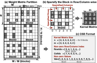
Figure 3. A novel structured sparse matrix (CSB) with its dedicated storage format, which benefits both the pruning flexibility and hardware parallelism.

3.1.1. Definition of CSB

We propose the compressed structured block (CSB), a novel structured sparse matrix for model pruning that benefits both the pruning flexibility and the hardware parallelism in inference acceleration. Fig. 3 illustrates the CSB matrix and the dedicated storage format. As Fig. 3(a), we consider the CSB-structured matrix (with a size of $W\times H$) to be composed of multiple blocks with the size $M\times N$. Each block is sparsified in the row/column-wise, as Fig. 3(b), in which the certain rows/columns are set to zero as a whole. By doing so, the non-zero elements are located at the cross-points of the un-sparsified rows/columns only. A significant benefit of this structured sparsity is the non-zero elements in each block compose a dense kernel matrix that provides a higher potential for parallel hardware acceleration than the random sparsity. Corresponding to this particular sparsity, a new sparse matrix format is developed for efficient storage and computation. As Fig. 3(c), the CSB-format contains five arrays in three groups, (i) array $\mathtt{n\{\}}$ and $\mathtt{m\{\}}$ are the row and column counts of the kernel matrix in each block; (ii) array $\mathtt{RowIdx\{\}}$ and $\mathtt{ColIdx\{\}}$ store the index of un-sparsified (non-zero) rows and columns, respectively; Note that, the index count for each block equals to the corresponding value in $\mathtt{n\{\}}$ or $\mathtt{m\{\}}$; (iii) the non-zero values in successive blocks (row-major order) are concatenated and stored continuously in the array $\mathtt{Val\{\}}$. Because the inference computation accesses the sparse blocks in sequential, the offset for arbitrary access is omitted in the CSB-format.

3.1.2. Advantages and Challenges of Pruning with CSB

We adopt the CSB structured sparsity in pruning the RNN models, which integrates two-fold advantages of both the non-structured pruning and coarse-grained structured pruning in Fig. 2. On one hand, CSB provides adequate pruning flexibility, because each block is pruned independently, and the pruning rate varies among blocks that helps to preserve the weights with important information. Physically, each element in the weight matrix represents the synapses (connection) between input neurons (matrix column) and output neurons (matrix row). The pruning process is zeroing the synapses between two neurons without a strong connection. The CSB pruning automatically groups the strongly-connected neurons into blocks with high density while leaving the weakly-connected ones in the low-density blocks. Further, the pruning granularity is adjustable via changing the block size; Such that different weight matrices in RNN model can be pruned with various granularities. The above flexibilities enable a high pruning rate while maintaining the model accuracy. On the other hand, the un-pruned weight values in each block compose a dense kernel matrix that makes the inference computation friendly to parallel hardware. Nevertheless, the blocks may have different-sized kernel matrices that result in a workload imbalance issue while mapping computation of blocks to parallel hardware. This paper carefully addresses this issue with an architecture-compilation co-design in §4 and §5.

3.2. CSB Pruning Flow with ADMM

input : un-pruned RNN model $\mathbf{W}$; lossless accuracy $accu$,

block size in CSB $M\times N$; weight matrix size $W\times H$

initial pruning rate $initPR$

initial step of pruning rate $initPRStep$

output :  maximally compressed model with CSB pruning $\mathbf{Z}$

// Initialization.

$\mathbf{U}=\mathbf{0}$; $\mathbf{Z}=\mathbf{W}$; $\mathbf{W}^{*}=\mathbf{W}$; Flag =False

PruneRate =$initPR$; StepPruneRate =$initPRStep$

// Progressive iteration.

repeat

       foreach t $\in$ $[0,100)$ // Re-train and Pruning Epoch.

       do

             // Solve Eqn. 4 in ADMM (1st subproblem)

             $\mathbf{W}^{*}$=SGDTrain($\mathbf{W}^{*},\mathbf{U},\mathbf{Z}$)

             // Solve Eqn. 5 in ADMM (2nd subproblem)

             // Project weight matrix to CSB pattern $\mathbf{S}$

             $\mathbf{Z}_{i,j}$=Partition($\mathbf{W}^{*}+\mathbf{U}$), $i\in[0,\frac{W}{M})$, $j\in[0,\frac{H}{N})$

             foreach $j$ $\in$ $[0,H/N)$ do

                   $\mathbf{Z}_{:,j}$=RowPrune($\mathbf{Z}_{:,j}$, $1-\sqrt{1-\textnormal{{PruneRate}}}$)

            foreach $i$ $\in$ $[0,W/M)$ do

                   $\mathbf{Z}_{i,:}$=ColumnPrune($\mathbf{Z}_{i,:}$, $1-\sqrt{1-\textnormal{{PruneRate}}}$)

            $\mathbf{U}=\mathbf{U}+\mathbf{W}^{*}-\mathbf{Z}$ // Update $\mathbf{U}$

            

      // Set progressive pruning rate.

       if Eval($\mathbf{Z}$)$<accu$ then

             Flag =True

             StepPruneRate =StepPruneRate/$2$

             PruneRate =PruneRate-StepPruneRate

      else

             if Flag then

                   StepPruneRate =StepPruneRate/$2$

            PruneRate =PruneRate +StepPruneRate

      

until StepPruneRate $\leq\frac{1}{4}initPRStep$ & Eval($\mathbf{Z}$)$\geq accu$;

Algorithm 1 Auto Lossless CSB Pruning with ADMM

With the ADMM-based pruning technique in §2.2.2, the weight matrices can be pruned to an arbitrary sparse pattern by defining the constraint $\mathbf{S}$ and applying the pattern-specific projection in Eqn. 6. To obtain the RNN model with CSB pattern, we develop the CSB pruning algorithm following the ADMM principle. Further, the maximum pruning rate under lossless constraint is automatically achieved via the progressive pruning. The entire CSB pruning flow is presented in Algorithm 1 with carefully specified annotations. Initially, the baseline model (with dense weight matrix $\mathbf{W}$) is obtained via classical SGD training and input to the flow. Note that the bias vector ($\mathbf{b}$) is omitted as the CSB pruning flow does not touch it. The lossless accuracy ($accu$) is given as the constraint of the progressive pruning. Two input parameters, initial pruning rate ($initPR$) and initial step of pruning rate reduction ($initPRStep$) are set for tuning the pruning rate in the progressive flow. We use the progressive increase manner in approaching the maximum value of lossless pruning rate. Therefore, we set $initPR$ to a small value (e.g., $4\times$) as the starting point, which surely meets the lossless constraint. The variables $\mathtt{PruneRate}$ and $\mathtt{StepPruneRate}$ are initialized to $initPR$ and $initPRStep$, respectively, at the beginning. In each progressive iteration, the flow performs re-training and pruning on the model with multiple epochs (e.g., $100$ in Algorithm 1) to obtain the CSB-formatted weight matrix ($\mathbf{Z}$) with the ADMM-pruning fashion. In each epoch, two subproblems are alternatively solved following the principle of the ADMM-pruning technique in §2.2.2. The function $\mathtt{SGDTrain}$ updates the weights with classical SGD ($1$st subproblem, Eqn. 4), and the subsequent process prunes the weight matrix and projects it to CSB-constrained set ($2$nd subproblem, Eqn. 5). The process in Algorithm 1 details the projection corresponding to the general representation in Eqn. 6. First, the weight from $\mathtt{SGDTrain}$ is partitioned to multiple blocks $\mathbf{Z}_{i,j}$ following the CSB method in §3.1. Then the $\mathtt{RowPrune}$ process is applied to each block-column independently. Specifically, for each block-column, the $\ell_{2}$-norm (accumulate the square of all elements) of each row (with the size of $M$) is obtained; Then, a row-wise pruning is conducted referring to the $\ell_{2}$-norm values. Subsequently, the $\mathtt{ColumnPrune}$ is applied to each block-row with the same behavior to $\mathtt{RowPrune}$. Note that the pruning rate in both $\mathtt{RowPrune}$ and $\mathtt{ColumnPrune}$ is $1-\sqrt{1-\mathtt{PruneRate}}$, which results in the target $\mathtt{PruneRate}$ after the combined processes. Once the CSB-formatted weight matrix $\mathbf{Z}$ is obtained, it will be sent to $\mathtt{SGDTrain}$ of the next epoch, along with un-pruned weight matrix $\mathbf{W}^{*}$ and accumulated difference matrix $\mathbf{U}$. With multiple epochs, weight $\mathbf{Z}$ will eventually meet the CSB pattern constraints and achieve good accuracy.

After each progressive iteration, the CSB pruned model is evaluated ($\mathtt{Eval}$($\mathbf{Z}$)) and compared to the lossless $accu$. The $\mathtt{PruneRate}$ is increased by $\mathtt{StepPruneRate}$ in the next iteration if the $accu$ is achieved. Once $\mathtt{Eval}$$(\mathbf{Z})<accu$, the model is over-pruned and the optimum pruning rate is just between the $\mathtt{PruneRate}$ of the two neighboring iterations. Therefore, we reduce $\mathtt{StepPruneRate}$ by half and reduce the $\mathtt{PruneRate}$ by this new step to further approach the optimum point. The progressive CSB pruning flow terminates until the pruning rate reaches a target precision. For instance, as the last line in Algorithm 1, the flow terminates when the pruning rate precision ($\mathtt{StepPruneRate}$) $\leq$ $\frac{1}{4}initPRStep$.

4. Unified Architecture for CSB-RNN

4.1. Overview of Acceleration Framework

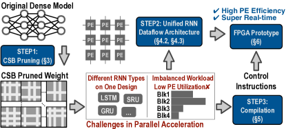
Figure 4. Overview of CSB RNN acceleration framework, including (i) CSB pruning algorithm, (ii) unified RNN dataflow architecture, (iii) workload compilation with CSB pruned model.

An overview of the CSB-RNN acceleration framework is illustrated in Fig. 4. Although the CSB pruning ($\mathtt{STEP1}$) shrinks the model size and therefore reduces the computation in inference, parallel hardware acceleration is still in demand to achieve realtime performance. The challenges in accelerating CSB-RNN are two-fold. First, the architecture should be adaptive to various RNN cell types, i.e., LSTM, GRU, etc. Second, the kernel matrix in fine-grained blocks may not provide enough inner-block parallelism for large-scale hardware. To further improve the concurrency, inter-block parallelism should be leveraged. However, the pruned blocks may have different sparsities, leading to the workload imbalance issue for inter-block parallelism, which usually causes a low utilization of processing element (PE). To address these challenges, CSB-RNN proposes an architecture-compilation co-design. In the architecture aspect ($\mathtt{STEP2}$), we propose a unified RNN dataflow architecture that is programmable for different RNN cell types (§4.2); In particular, a novel $\mathtt{CSB}$-$\mathtt{Engine}$ is designed with the support of workload sharing and is equipped in CSB-RNN architecture to address the workload imbalance issue (§4.3). In the compilation aspect ($\mathtt{STEP3}$), we define control instructions for the hardware and propose the compilation algorithms to conduct the particular RNN type computation and balanced workload scheduling (§5).

4.2. Programmable RNN Dataflow Architecture

To generalize the architecture for different RNN cell types, we investigated the existing RNN cells and extracted the arithmetic primitives, which compose the RNN computation in a dataflow fashion. Fig. 5 presents the hardware components in this architecture, where each operation unit serves the corresponding arithmetic primitive. In particular, the $\mathtt{CSB}$-$\mathtt{Engine}$ computes the main workload, MVM, with the weight matrices after CSB pruning (CSB-MVM). The units $\mathtt{\times}$, $\mathtt{+}$ are the element-wise multiplication and addition. $\mathtt{\delta}$ and $\mathtt{\theta}$ operate the activation functions Sigmoid and Tanh, respectively. The datapaths (arrows on Fig. 5) interconnect the operation units and on-chip buffers, which transmit the intermediate results and compose the dataflow graph for RNN cell computation. Importantly, RNN dataflow architecture provides the programmable datapath (red arrows on Fig. 5). Thus, the proper operation units can be interconnected by programming control instructions for a particular RNN cell type.

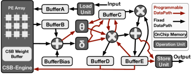
Figure 5. RNN dataflow architecture. Operation units serve the RNN arithmetic primitives; The programmable datapaths construct the proper dataflow for target RNN cell via instructions.

4.3. CSB-Engine

The CSB pruning scheme greatly shrinks the weight matrix size and therefore reduces the main workload in inference. Although the fine-grained structure of CSB contributes to the regularity and makes efficient hardware acceleration possible, it is still challenging to design a parallel architecture that can fully exploit the benefits of CSB pruning. The challenges in an efficient $\mathtt{CSB}$-$\mathtt{Engine}$ design are two-fold. First, both the inner-block and inter-block parallelism should be fully exploited, as the regular inner-block computation provides very limited concurrency with small block size. Second, the inter-block workload imbalance issue exists due to the sparsity varies among blocks. The following §4.3.1 and §4.3.2 address these two challenges, respectively.

4.3.1. Hierarchical Design for Inner- and Inter-Block Parallelism

As illustrated in Fig. 6, the $\mathtt{CSB}$-$\mathtt{Engine}$ design is in a two-level hierarchy, processing element ($\mathtt{PE}$) level and $\mathtt{PEGroup}$ level. The hardware instances in each level are organized in a 2D fashion that the architecture is composed of $K\times L$ $\mathtt{PEGroup}$s, and each $\mathtt{PEGroup}$ contains $P\times Q$ $\mathtt{PE}$s. The parallel $\mathtt{PE}$s inside one $\mathtt{PEGroup}$ process inner-block multiplication concurrently, while the $\mathtt{PEGroup}$s computing different blocks in parallel (inter-block parallelism).

Inside each $\mathtt{PEGroup}$, because the size of CSB kernel matrix ($m\times n$) might be larger than that of $\mathtt{PE}$ array ($P\times Q$), multi-pass processing is required to handle the entire block. Thus, each $\mathtt{PEGroup}$ contains a $\mathtt{NeuronAccumBuffer}$, which stores the partial results and sums up with the accumulation of horizontal $\mathtt{PE}$s in each pass. The input neurons required by the current block are preloaded to the $\mathtt{BlockNeuronBuffer}$ and broadcasted to the $\mathtt{PE}$ array. Each $\mathtt{PE}$ column shares the same input neuron as the unpruned weights are vertically aligned in the structured block with CSB pruning. Importantly, the $\mathtt{WeightBuffer}$ provides the CSB-formatted weight (Fig. 3), including the weight values (kernel matrix) for $\mathtt{PE}$s, column index for $\mathtt{BlockNeuronBuffer}$ to read the proper input neuron, row index for $\mathtt{NeuronAccumBuffer}$ to accumulate the multiplication-results to proper address in $\mathtt{NeuronAccumBuffer}$, and the kernel matrix size ($m\times n$) for the $\mathtt{PEGroup}$ control logic which conducts proper pass count in both axes.

In the higher-level of the design hierarchy, the $\mathtt{PEGroup}$s process blocks in the row-major order. The $\mathtt{PEGroup}$s in one column concurrently compute the vertical blocks. Therefore, the $\mathtt{PEGroup}$s in one column share the same partition of input neuron vector, while multi-ports are provided on $\mathtt{BlockNeuronBuffer}$ for concurrent access. Similarly, the blocks in horizontal axis are mapped to $\mathtt{PEGroup}$s in the same row, with multi-pass processing. After the computation of each block-row, the results in $\mathtt{NeuronAccumBuffer}$s are accumulated in horizontal and output to $\mathtt{ReorderLogic}$ to obtain the output neuron vector.

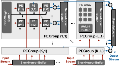
Figure 6. Two-level hierarchical organization of CSB-Engine for the main workload (CSB-MVM) computation.

4.3.2. Inter-PEGroup Workload Sharing

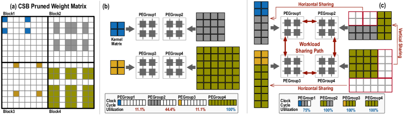
Figure 7. Inter-block workload imbalance issue occurs when mapping the CSB pruned matrix (a) to the vanilla (basic) CSB-Engine (b), which results in a low hardware utilization. We propose the workload sharing technique that significantly increases the utilization and reduces the time consumption, as demonstrated in (c).

Workload Imbalance Challenge: The blocks in CSB pruned model may have different-sized kernel matrices, and the resultant inter-block workload imbalance brings challenges to exploit the inter-block parallelism on hardware. As Fig. 7(b) demonstrates, with the straightforward design, the workload imbalance issue results in low utilization of $\mathtt{PEGroup}$s. The presented MVM workloads are allocated to $2\times 2$ $\mathtt{PEGrounp}$s that each contains $4$ $\mathtt{PE}$s. During the execution, $\mathtt{PEGroup1}$-$\mathtt{3}$ enter the idle state before the $\mathtt{PEGroup4}$ accomplishes its workload, which results in a severe under-utilization of the overall hardware. In fact, the imbalanced sparsity naturally exists in the RNN models. However, existing works (Han et al., 2017; Cao et al., 2019) relieve the hardware pain by pruning the model with a region-balanced sparsity compulsively. As a result, the neglect of natural sparsity-imbalance significantly harms the pruning ratio and model accuracy. By contrast, we handle this issue by improving the architecture with the workload sharing technique.

Inter-PEGroup Workload Sharing: The concept of workload sharing is illustrated in Fig. 7(c). Each $\mathtt{PEGroup}$ processes not only the originally allocated block but also a partition of block from the neighboring $\mathtt{PEGroup}$, which is arranged with a heavier workload. In the hardware aspect, as Fig. 7(c), dedicated workload sharing paths (red arrows) are set for the inter-$\mathtt{PEGroup}$ data transmission, and the interconnection adopts the torus topology in both dimensions. With the hardware support of workload sharing, $\mathtt{PEGroup4}$ migrates the extra workloads to $\mathtt{PEGroup2}$ and $\mathtt{PEGroup3}$; And $\mathtt{PEGroup2}$ migrates the Block$2$ workload partition to $\mathtt{PEGroup1}$. That significantly balances the workload and improves the utilization. Considerations in the workload sharing design are two-fold. (i) The input neurons should be sharable between the $\mathtt{PEGroup}$s; (ii) The output neuron accumulation should be performed inter-$\mathtt{PEGroup}$s. We discuss these issues and our strategies within two cases, in which the workload is shared between neighboring $\mathtt{PEGroup}$s in horizontal or in vertical, respectively. For the horizontal sharing case, an extra data port is set on the $\mathtt{BlockNeuronBuffer}$ to solve the issue (i), which enables the $\mathtt{PEGroup}$ to access input neurons from the neighboring $\mathtt{PEGroup}$ in horizontal. The issue (ii) is naturally solved by the hierarchical $\mathtt{CSB}$-$\mathtt{Engine}$ design, as the $\mathtt{PEGroup}$ can store the partial results of the shared workload partition in its local $\mathtt{NeuronAccumBuffer}$, which will be accumulated in horizontal after processing the entire block-row. For the vertical sharing case, the $\mathtt{PEGroup}$-column shares the same $\mathtt{BlockNeuronBuffer}$, thus the issue (i) is naturally solved by hardware. About the issue (ii), the $\mathtt{PEGroup}$ should accumulate the vertically shared workload to its original $\mathtt{PEGroup}$, as the vertical $\mathtt{PEGroup}$s compute different block-rows that cannot be accumulated in a mixed manner. However, concurrent accumulation to one address in $\mathtt{NeuronAccumBuffer}$ leads to the read-after-write (RAW) data hazard. To address this issue, an accumulation path is set between vertical $\mathtt{PEGroup}$s and connected to the adder, which accepts parallel results from neighboring $\mathtt{PEGroup}$s, sums up and stores to the $\mathtt{NeuronAccumBuffer}$ for one shot. With the hardware support on workload sharing, we propose the compilation scheme in next section that schedules the partition and sharing by analyzing the CSB pruned matrix and generates the instruction to control the hardware-sharing behavior.

5. Compilation for CSB Pruned Model

The proposed RNN dataflow architecture is controlled by the pre-compiled instructions. The instruction set includes the macro-instruction and micro-instruction, where the former one conducts the operation units (in Fig. 5) for the proper RNN dataflow (cell type); and the later one instructs the $\mathtt{CSB}$-$\mathtt{Engine}$ with inter-$\mathtt{PEGroup}$ workload sharing behavior as described in §4.3.2. Correspondingly, the compilation is composed of two phases, RNN dataflow compilation (§5.1) and workload sharing scheduling (§5.2).

5.1. RNN Cell to Dataflow Architecture

5.1.1. Macro-Instruction Set

We define the macro-instruction set for our RNN dataflow architecture (§4.2). As Fig. 8, the micro-instruction is composed of multiple sections, that each section provides control signals for corresponding RNN primitive hardware. All sections are concatenated to form a very long instruction word (VLIW) item. Note that each section contains $\mathtt{Count}$ operand to indicate the size of workload for corresponding hardware primitive. Thus, one VLIW instruction is regarded as accomplished until all hardware primitives finish the workload. The operands in each instruction section are classified into two types, the $\mathtt{Count}$ type controls the hardware iteration count, and the other operands indicate the proper data source or destination for each primitive. For the first type, the value of $\mathtt{Count}$ in element-wise operation units (only $\mathtt{CSB}$-$\mathtt{Engine}$ excluded) is measured by data element as these units perform element-wise operation. Differently, the $\mathtt{CountH/V}$ in $\mathtt{CSB}$-$\mathtt{Engine}$ section represents the horizontal/vertical block iteration counts over the entire $\mathtt{CSB}$-$\mathtt{Engine}$ in processing the particular weight matrix. For the second operand type, $\mathtt{Addr(Memory)}$ and $\mathtt{Addr(Buffer)}$ give the access address of external memory (normally DRAM) and built-in buffers in the architecture, respectively. Importantly, the programmable datapaths in the architecture (Fig. 5) are indexed, and the $\mathtt{DataFlowIdx}$ is set in the operand to indicate the proper data source or destination for hardware primitive. With the above settings, RNN models with various cell types can be translated to several VLIW instructions that are repetitively executed during RNN inference.

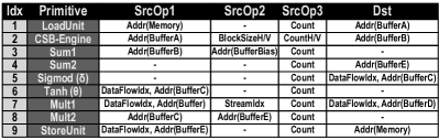
Figure 8. Macro-instruction set (VLIW-like) for RNN dataflow architecture that constructs proper arithmetic dataflow for different RNN cell types.

5.1.2. Macro-Instruction Compilation

The objective of compilation is to minimize the VLIW instruction count that maximizes the utilization of operation units. We invoke the list scheduling method (Lam, 1988) that is usually applied in VLIW compilation. The RNN model with a particular cell type is translated to the directed acyclic graph (DAG), in which the nodes represent the arithmetic primitives and the edges are data dependencies. In the list scheduling, we adopt the as soon as possible (ASAP) strategy that the operation nodes are mapped to the corresponding hardware resources once the resource is available and the dependency edge is ready. With the proper operation units and interconnection in the RNN dataflow architecture, the macro-instruction compilation can quickly achieve an optimum point, in which the processing throughput is bounded by the main workload (CSB-MVM) on $\mathtt{CSB}$-$\mathtt{Engine}$.

5.2. Workload Scheduling on CSB-Engine

5.2.1. Micro-Instruction Set

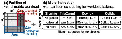
Figure 9. Micro-instruction indicates the kernel matrix workload and the scheduling of partition for workload balancing.

The micro-instructions are generated for each $\mathtt{PEGroup}$ individually, which control the CSB-MVM operations on $\mathtt{CSB}$-$\mathtt{Engine}$. Specifically, the micro-instruction contains the CSB-compression information (i.e., kernel matrix size, row- and column-index in Fig. 3(c)) for the block workload allocated to the certain $\mathtt{PEGroup}$. In particular, the kernel matrix workload is partitioned to three submatrices and shared to neighboring $\mathtt{PEGroup}$s (as Fig. 9(a)), the micro-instructions for one block iteration include three items, (i) local workload that is originally allocated, excluding the portion shared to other $\mathtt{PEGroup}$s; (ii) workload shared from the neighboring $\mathtt{PEGroup}$ in horizontal; (iii) workload shared from the neighboring $\mathtt{PEGroup}$ in vertical. The micro-instruction contains $4$ operands, as Fig. 9(b). The operand $\mathtt{Sharing}$ gives a flag (local/horizontal/vertical) to indicate the data source, where local means the input and output neurons are in local $\mathtt{PEGroup}$; horizontal (sharing) indicates the input neurons should be read from the $\mathtt{BlockNeuronBuffer}$ of left $\mathtt{PEGroup}$; Vertical (sharing) means the output should be accumulated to the $\mathtt{NeuronAccumBuffer}$ of upper $\mathtt{PEGroup}$. The operand $\mathtt{TripCount}$ gives the size of workload. Note that, for each block, the kernel matrix is divided to tree regular partitions as Fig. 9(a), for local (no-sharing), vertical- and horizontal-sharing, respectively. The sizes of partitioned matrices are denoted as $m^{\prime}\times n^{\prime}$, $\Delta m_{v}\times\Delta n_{v}$, $\Delta m_{h}\times\Delta n_{h}$, which are turned to $\mathtt{TripCount}$ values in the three micro-instruction items. The operands $\mathtt{RowIdx}$ and $\mathtt{ColIdx}$ provide the non-zero row and column indices of each submatrix. Note that each micro-instruction item may contain multiple $\mathtt{RowIdx}$ and $\mathtt{ColIdx}$ corresponding to the $\mathtt{TripCount}$ value. Further, these two operands are stored in individual instruction memories that are read and reused periodically in the submatrix computation.

5.2.2. Micro-Instruction Compilation

The compilation of micro-instruction is essentially searching the workload partition scheme to achieve the optimal balance, which facilitates a higher hardware utilization (efficiency). Specifically, the compiler analyzes the weight matrices and selects the proper partition variables (as Fig. 9(a)) for each kernel matrix. Every $K\times L$ blocks (one block iteration) are analyzed individually, which are executed on $\mathtt{PEGroup}$s in concurrent. Within one block iteration, each $\mathtt{PEGroup}$ is supposed to take the equivalent workload after balancing.

We regard the search of optimal partition variable as a satisfiability modulo theories (SMT) problem (Winter and Smith, 1992), which searches the feasible solutions in the constrained region. The existing SMT solver (De Moura and Bjørner, 2008) takes the constraints with logic programming and gives the satisfiability (existence of solution) and feasible solutions. In the compilation for each block iteration, we declare the integer variables including $m^{\prime}(k,l)$, $n^{\prime}(k,l)$, $\Delta m_{h}(k,l)$, $\Delta n_{h}(k,l)$, $\Delta m_{v}(k,l)$, $\Delta n_{v}(k,l)$, where $k\in[1,K]$ and $l\in[1,L]$. The constraints are represented with the constraint logic programming (CLP), in which each clause gives a specific search limitation. The CLP in compilation is listed in Eqn. 7, where $\wedge$ represents logic AND and $\vee$ represents OR. $\mathtt{CLP}_{\mathrm{1,2}}$ constraint the feasible search region, as the size of the partitioned workload should $\leq$ kernel matrix size ($m\times n$). $\mathtt{CLP}_{\mathrm{3,4}}$ guarantee regular partitions as Fig. 9(a). $\mathtt{CLP}_{\mathrm{5}}$ determines the values of $m^{\prime}$ and $n^{\prime}$. To improve the $\mathtt{PEGroup}$ utilization, we set $\mathtt{CLP}_{\mathrm{6}}$ constraint that the size of partition workload should be integer-multiple of the $\mathtt{PEGroup}$ size. Thus, the $\mathtt{PE}$s are fully utilized on the shared workload partition. Also, it helps to shrink the search space and speed up the compilation. Within the idealized situation, each $\mathtt{PEGroup}$ is scheduled with workload that is the average value over all $\mathtt{PEGroup}$s in the current block iteration. Otherwise, the $\mathtt{PEGroup}$ with maximum workload determines the run time (clock cycle) for this iteration. $\mathtt{CLP}_{\mathrm{7}}$ gives the constraint on the maximum workload that, to all $\mathtt{PEGroup}$s, the exceeding part of scheduled workload to the average value ($avg$) should $\leq$ $margin$, which is given before search. The last $\mathtt{CLP}$ combines all above constraints to a conjunctive form, which is subsequently sent to SMT-solver for a feasible solution.

$$\mathtt{CLP}_{\mathrm{1}}: \{0\leq\Delta m_{h}(k,l)\leq m(k,l)\}\wedge\{0\leq\Delta n_{h}(k,l)\leq n(k,l)\}$$

$$\mathtt{CLP}_{\mathrm{2}}: \{0\leq\Delta m_{v}(k,l)\leq\lfloor m(k,l)/2\rfloor\}\wedge\{0\leq\Delta n_{v}(k,l)\leq n(k,l)\}$$

$$\mathtt{CLP}_{\mathrm{3}}: \{\Delta m_{h}(k,l)=m(k,l)\}\wedge\{\Delta n_{v}(k,l)+\Delta n_{h}(k,l)=n(k,l)\}$$

$$\mathtt{CLP}_{\mathrm{4}}: \{\Delta n_{v}(k,l)=n(k,l)\}\wedge\{\Delta m_{h}(k,l)+\Delta m_{v}(k,l)=m(k,l)\}$$

$$\mathtt{CLP}_{\mathrm{5}}: \{m^{\prime}(k,l)=m(k,l)-\Delta m_{v}(k,l)\}\wedge\{n^{\prime}(k,l)=n(k,l)-\Delta n_{h}(k,l)\}$$

$$\mathtt{CLP}_{\mathrm{6}}: \{\Delta m_{h}(k,l)\%P=m_{v}^{\prime}(k,l)\%P=0\}\wedge\{\Delta n_{h}(k,l)\%Q=n_{v}^{\prime}(k,l)\%Q=0\}$$

$$\mathtt{CLP}_{\mathrm{7}}: |~{}(m^{\prime}(k,l)\times n^{\prime}(k,l)+\Delta m_{h}(k,l-1)\times\Delta n_{h}(k,l-1)$$

$$+\Delta m_{v}(k-1,l)\times\Delta n_{v}(k-1,l))-avg~{}|\leq margin$$

(7) $$\mathtt{CLP}: \mathtt{CLP}_{\mathrm{1}}\wedge\mathtt{CLP}_{\mathrm{2}}\wedge(\mathtt{CLP}_{\mathrm{3}}\vee\mathtt{CLP}_{\mathrm{4}})\wedge\mathtt{CLP}_{\mathrm{5}}\wedge\mathtt{CLP}_{\mathrm{6}}\wedge\mathtt{CLP}_{\mathrm{7}}$$

input : CSB pruned weight matrix $\mathbf{W}_{csb}$;

block size in CSB $M\times N$; weight matrix size $W\times H$;

size of each $\mathtt{PEGroup}$ $P\times Q$; $\mathtt{PRGroup}$ count $K\times L$

output : Micro-instruction list $MicroInst$

// Temporal block iterations in vertical.

for $i\leftarrow 1$ to $\lceil H/N/K\rceil$  do

       // Temporal block iterations in horizontal.

       for $j\leftarrow 1$ to $\lceil W/M/L\rceil$  do

             $margin$=0

             // $\forall k\in[1,K]$, $\forall l\in[1,L]$.

             [$m(k,l),n(k,l)$, $avg$]=Analyze ($\mathbf{W}_{csb}$,i,j)

             // Search with multiple rounds.

             repeat

                   CLP =BuildCLP ($m(k,l),n(k,l)$, $avg$, $margin$)

                   // Give solution if satisified.

                   [Satisfiability, PartitionVar ] = SMTSolver (CLP)

                   $margin$+=$P\times Q$

            until Satisfiability =True;

            $MicroInst$=Append ($MicroInst$, PartitionVar)

      

Algorithm 2 Micro-Instruction Compilation

Based on the above formulation, we propose the compilation scheme in Algorithm 2 that seeks out the optimal scheduling solution. For a given CSB formatted weight matrix $\mathbf{W}_{csb}$, the compiler partitions it to $\lceil W/M/L\rceil\times\lceil H/N/K\rceil$ temporal block iterations and schedules each iteration individually. Before the multi-round search, the compiler firstly analyzes the weight partition for current block iteration that gives the kernel matrix size ($m,n$) for each block and the average workload ($avg$). The $margin$ is initialized to $0$ that targets to schedule an idealized average workload on each $\mathtt{PEGroup}$. In the search round, $\mathtt{BuildCLP}$ constructs the constraints representation, which is input to $\mathtt{SMTSolver}$. In case the constraints cannot be satisfied ($\mathtt{Satisfiability}$ is False) over the feasible region, the $margin$ value is supposed to increase by $P\times Q$ in the next round. Once the SMT problem is satisfied, the search stops and the partition variables ($m^{\prime}$, $n^{\prime}$, $\Delta m_{v}$, $\Delta n_{v}$, $\Delta m_{h}$, $\Delta n_{h}$) for each $\mathtt{PEGroup}$ are assembled and appended to the micro-instruction list, that conducts the $\mathtt{CSB}$-$\mathtt{Engine}$ computation in a workload balanced fashion.

6. Evaluation

In this section, we first brief the implementation of the CSB-RNN framework (§6.1), and then give deep evaluations from the performance of CSB pruning algorithm (§6.2) to the improvement with the architecture-compilation co-design (§6.3). Meanwhile, $10$ mainstream RNN models from multi-domains are invoked as the evaluation benchmarks and presented in Table 1, in which we also list the non-structured pruning rates as the theoretical optimum.

6.1. Implementation and Experiments Setup

The CSB pruning flow was implemented with PyTorch (Paszke et al., 2019), a framework for deep learning model development. The benchmark models were first trained with the SGD and the accuracy is regarded as the lossless target value in the subsequent CSB pruning. These baseline models were fed in the CSB pruning flow and get compressed with the lossless constraints. In regarding the architecture-compilation co-design, the proposed RNN dataflow architecture was realized with Verilog RTL and implemented on an FPGA vendor evaluation board (Xilinx-ZCU$102$), on which the FPGA contains enough resources for our architecture with different design scales. The compiler was implemented in C++ with the strategies in §5 and Z3 (De Moura and Bjørner, 2008) as the SMT solver. With the CSB pruned model, the compiler dumps the macro-instructions (§5.1) to build the proper RNN dataflow and micro-instructions (§5.2) for the workload balancing. These instructions are loaded to the RNN dataflow architecture before processing sequence continuously. With regard to the detailed hardware efficiency (i.e, $\mathtt{CSB}$-$\mathtt{Engine}$ utilization), cycle-level RTL simulation was performed to profile the inference behavior.

Table 1. Benchmark Models in CSB-RNN Evaluation

App.	Abbr.	Applications	Dataset	#Layer	RNN Cell	Layer	#Input	#Hidden	Evaluation Metric	Original Model		Non-Structued Pruning
Idx.						Index	Neuron	Neuron		#Weight+Bias	Result	PruneRate	#Weight	Result
1	$\mathtt{MT1}$	Machine Translation	PTB(Marcus et al., 1993)	2	LSTM(Hochreiter and Schmidhuber, 1997)	1	128	256	Perplexity (PPL, lower is better)	393K+1K	110.89	13.2$\times$	29.8K	111.62
						2	256	256		524K+1K		13.2$\times$	39.7K
2	$\mathtt{MT2}$	Machine Translation	PTB(Marcus et al., 1993)	2	LSTM(Hochreiter and Schmidhuber, 1997)	3	1500	1500	Perplexity (PPL)	18M+6K	80.66	16.3$\times$	1.1M	82.33
						4	1500	1500		18M+6K		16.3$\times$	1.1M
3	$\mathtt{SR1}$	Speech Recognition	TIMIT(Garofolo et al., 1993)	2	LSTMP(Sak et al., 2014)	5	153	1024	Phoneme Error Rate (PER, lower is better)	3.25M+4K	19.39%	14.5$\times$	224.0K	19.70%
						6	512	1024		4.72M+4K		14.5$\times$	325.4K
4	$\mathtt{SR2}$	Speech Recognition	TIMIT(Garofolo et al., 1993)	2	GRU(Cho et al., 2014)	7	39	1024	PER	3.3M+3K	19.24%	21.7$\times$	150.5K	19.80%
						8	1024	1024		6.3M+3K		21.7$\times$	289.9K
5	$\mathtt{SR3}$	Speech Recognition	TIMIT(Garofolo et al., 1993)	2	Li-GRU(Ravanelli et al., 2018)	9	39	512	PER	564.2K	16.87%	7.1$\times$	79.5K	17.30%
						10	512	512		1M		7.1$\times$	147.7K
6	$\mathtt{SR4}$	Speech Recognition	TDIGIT(Leonard et al., 1993)	1	GRU(Cho et al., 2014)	11	39	256	Accuracy	226.6K+0.8K	99.98%	25.7$\times$	8.8K	99.21%
7	$\mathtt{SPP}$	Stock Price Prediction	S&P500(Indices, 2019)	2	LSTM(Hochreiter and Schmidhuber, 1997)	12	1	128	Normalized Price Dist. (lower is better)	66K+0.5K	0.47	4.1$\times$	16.1K	0.51
						13	128	128		131K+0.5K		4.1$\times$	32K
8	$\mathtt{SC1}$	Sentiment Classification	IMDB(Maas et al., 2011)	3	LSTM(Hochreiter and Schmidhuber, 1997)	14	32	512	Accuracy (higher is better)	1.11M+2K	86.37%	10.4$\times$	107.1K	85.65%
						15	512	512		2.1M+2K		10.4$\times$	201.6K
						16	512	512		2.1M+2K		10.4$\times$	201.6K
9	$\mathtt{SC2}$	Sentiment Classification	MR(Pang and Lee, 2005)	1	LSTM(Hochreiter and Schmidhuber, 1997)	17	50	256	Accuracy	313.3K+1K	78.23%	7.2$\times$	43.5K	76.31%
10	$\mathtt{QA}$	Question Answering	BABI(Weston et al., 2015)	3	LSTM(Hochreiter and Schmidhuber, 1997)	18	50	256	Accuracy	313.3K+1K	65.37%	7.9$\times$	39.7K	64.51%
						19	256	256		524.3K+1K		7.9$\times$	66.4K
						20	256	256		524.3K+1K		7.9$\times$	66.4K

6.2. Evaluation of CSB pruning Rate

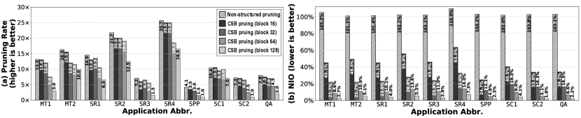
Figure 10. (a) shows the pruning rate comparison between non-structured pruning (optimum) and CSB pruning in different block sizes. (b) shows the normalized index overhead (NIO). Comparing (a) and (b), we gain the insight that CSB pruning dramatically reduces the NIO while maintaining a high pruning rate.

The CSB pruning is first evaluated in the aspect of pruning rate, which is a significant metric to score the model compression methods. Because the parameterizable block size determines the structural granularity in pruning, we present the attainable maximum pruning rate with various block sizes in §6.2.1. Further, comparison with the prior art RNN compression schemes is given in §6.2.2.

6.2.1. Selection of Optimum Structural Granularity

CSB pruning provides the flexibility that improves the pruning rate and also the hardware-friendly regularity. Importantly, a trade-off exists between these two targets that motivate the following investigation. Reducing the block size facilitates a more fine-grained pruning and thus a higher pruning rate. However, more individual blocks require extra storage for row and column index with the CSB-formatted weight matrix (Fig. 3). Therefore, we present both the attainable pruning rate and the index overhead with different block sizes in each benchmark model. The block is set to square with sizes of $16$, $32$, $64$, $128$, considering the weight matrix dimensions in different models. Note that for matrix with very small size (e.g., $256\times 39$ in $\mathtt{SR4}$), the short dimension ($39$) is partitioned to $Q$ blocks uniformly after padding a zero-column. Multiple layers in one model adopt the same pruning rate. The attainable pruning rate for each case is presented in Fig. 10(a); Further, the index overheads are divided by the corresponding weight count for normalization, and the values of the normalized index overhead (NIO) are presented in Fig. 10(b). Notably, the results with non-structured pruning are given for comparison (leftmost bar for each application); And its index overhead is obtained by compressing the non-structured weight matrices with the compressed sparse row (CSR) format.

As a result, the CSB pruning rate ranges from $3.5\times$ to $25\times$, which dramatically reduces the original model size by order of magnitude. With the growth of block size, the pruning rate decreases as the coarse-granularity block reduces the pruning flexibility. We note that, in all benchmarks, the CSB pruning is capable of reaching a maximum pruning rate with the block size of $16$ or $32$, which is close to non-structured pruning. In the aspect of NIO, the index overhead of non-structured pruning exceeds $100\%$, as at least one index is required for a non-zero element. Nevertheless, for CSB pruning, the NIO is below $50\%$ in most cases due to index reusability in the structured blocks. The NIO shows a significant decay while enlarging the block size. With the block size of $32$, the NIO declines to $\approx 20\%$, which is $1/5$ of that in non-structured pruning. Interestingly, we gain the insight that with a block size of $32$ and $16$, most models achieve the close pruning rate. For instance, $13\times$ and $12\times$ in $\mathtt{MT1}$; both are $20\times$ in $\mathtt{SR2}$. Therefore, the larger block size ($32$) is preferable for its low index overhead.

6.2.2. Comparison with Prior Art Compression Schemes

Table 2. Pruning Rate Comparison

Abbr.	Compression Technique	Prune Rate	Weight Width	Metric	Result	Impro- vement
$\mathtt{MT1}$	column pruning (Wang et al., 2019)	8$\times$	16-bit	PPL	112.73	1$\times$
	CSB pruning	12.5$\times$	16-bit		112.02	1.6$\times$
$\mathtt{MT2}$	row-column (Wen et al., 2018)	3$\times$	floating	PPL	82.59	1$\times$
	bank balanced (Cao et al., 2019)	5$\times$	16-bit		82.59	1.65$\times$
	CSB pruning	12$\times$	16-bit		82.33	3.9$\times$
$\mathtt{SR1}$	block circulant (Wang et al., 2018)	8$\times$	16-bit	PER	24.57%	1$\times$
	row balanced (Han et al., 2017)	8.9$\times$	16-bit		20.70%	1.1$\times$
	bank balanced (Cao et al., 2019)	10$\times$	16-bit		23.50%	1.3$\times$
	CSB pruning	13$\times$	16-bit		20.10%	1.6$\times$
$\mathtt{SR2}$	block circulant (Li et al., 2019)	8$\times$	16-bit	PER	20.20%	1$\times$
	CSB pruning	20$\times$	16-bit		20.01%	2.5$\times$
$\mathtt{SR4}$	column pruning (Gao et al., 2018)	14.3$\times$	16-bit	Accu	98.43%	1$\times$
	CSB pruning	23$\times$	16-bit		99.01%	1.6$\times$

The CSB pruning rate is further compared to the prior art RNN compression techniques in Table 2. The listed competitive techniques are proposed to enable a faster, hardware-friendly RNN inference with the compressed model. Note that these competitors quantized the weight to $16$-bit fixed-point numbers; Thus, we do the same quantization on CSB pruned model and report the corresponding results for a fair comparison. In Table 2, row-column (Wen et al., 2018) technique prunes each weight matrix as an entire block. Comparing to it, our fine-grained CSB pruning improves the compression rate to $3.9\times$. The row balanced (Han et al., 2017) or bank balanced (Cao et al., 2019) techniques compulsively train the model to a balanced sparse pattern; However, CSB pruning remains the natural unbalanced sparsity in RNN model and achieves a higher ($1.6\times$) pruning rate. Overall, the CSB pruning improves the pruning rate to $1.6\times$-$3.9\times$ of the existing schemes, while maintaining an even better model accuracy.

6.3. Evaluation of RNN dataflow Architecture with CSB Pruned Model

6.3.1. Hardware-resource Consumption

The hardware-resource consumption (cost) of the RNN dataflow architecture is given in Fig. 11, with various $\mathtt{CSB}$-$\mathtt{Engine}$ configs ($P$,$Q$,$K$,$L$ and max supported block size). Notably, the $\mathtt{CSB}$-$\mathtt{Engine}$ with different workload sharing configs, including no-sharing, vertical-sharing, horizontal-sharing, 2D-sharing, are synthesized individually to evaluate the hardware overhead on workload sharing technique. The consumption of hardware logic and memory from the FPGA vendor tool are presented in Fig. 11. The configurable logic block (CLB, left axis) is the FPGA building block for logic, which is used as the logic resource metric; The memory resource is given in megabit (Mb in the right axis). Note that most memory resource on our FPGA device is configured as the weight buffer, although they may not be fully used by small RNN models. The multiplier in each $\mathtt{PE}$ ($16$-bit fixed-point) is mapped to digital signal processor (DSP) on FPGA, and the DSP count in design is $\approx P\times Q\times K\times L$ that is omitted here. As a result, the hardware support of workload sharing costs an acceptable overhead, which is $11.6\%$, $3.8\%$, and $15.6\%$ for three sharing cases (vertical/horizontal/2D-sharing), respectively.

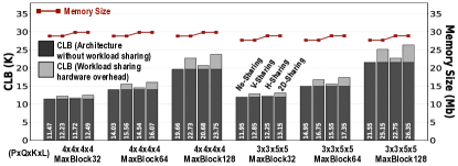
Figure 11. Hardware resource consumption with multi CSB-Engine configs.

6.3.2. Performance

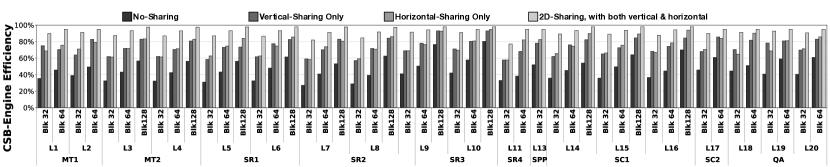
Figure 12. The efficiency (utilization) of the proposed architecture with different sharing strategies. The novel workload sharing technique significantly improves the average efficiency from $42\%$ (no-sharing) to $94\%$ (2D-sharing). This improvement fully exploits the benefits of fine-grained CSB pruning.

Due to the workload imbalance issue, the processing performance of RNN dataflow architecture, $\mathtt{CSB}$-$\mathtt{Engine}$ in specific, is not deterministic. Hardware efficiency, the ratio of effective computation on $\mathtt{PE}$s, is invoked to evaluate the improvement of our workload sharing technique. We obtained the $\mathtt{CSB}$-$\mathtt{Engine}$ efficiency by measuring the $\mathtt{PE}$ pipeline utilization using $10$ benchmarks listed in Table 1 with different design choices of workload sharing. Moreover, CSB pruned models with different block sizes are used to evaluate the impact of block size on efficiency. The efficiency is measured layer-by-layer on hardware with $4\times 4$ $\mathtt{PEGroup}$s and each contains $4\times 4$ $\mathtt{PE}$s. The results are presented in Fig. 12. Overall, for the $\mathtt{CSB}$-$\mathtt{Engine}$ without workload sharing, the efficiency is $42\%$ on average, which results from the imbalanced workload (sparsity) of blocks. The single dimensional sharing (vertical or horizontal) improves the efficiency to an average of $72\%$. After the 2D-sharing is adopted, the efficiency is further improved to $94\%$ on average, i.e., only $6\%$ execution time of $\mathtt{CSB}$-$\mathtt{Engine}$ is invalid. This $6\%$ pipeline gap is inevitable, as a few extremely imbalanced sparsity exists in some weight matrices. For instance, we found diagonal dense matrix exists that the blocks on the matrix diagonal contain significant workload compared to other blocks. In this case, the workload sharing path in the current design is not enough, while adding more sharing paths brings extra hardware costs.

Comparing the efficiency within the same layer but different pruning block sizes, it is apparent that the smaller block size is applied, the lower hardware efficiency $\mathtt{CSB}$-$\mathtt{Engine}$ can achieve, particularly in the no-sharing $\mathtt{CSB}$-$\mathtt{Engine}$ cases. This is because the small block includes less workload (with the same pruning rate) but more temporal block iterations, which lead to $\mathtt{PE}$ idle more easily. As mentioned in §6.2.1, using smaller block sizes in compression guarantees higher model pruning rates, which benefits are significantly encroached by the performance degradation with small compression block in the no-sharing cases. Nevertheless, we gain the insight that our architecture-compilation co-design for 2D-sharing cases significantly subdues the degradation. For instance, in Layer-2 (L2) of $\mathtt{MT1}$ case, the no-sharing degradation from block-64 to block-32 is $12\%$, while it is reduced to $3\%$ by the 2D-sharing. On average, the degradation is reduced from $15\%$ to $4\%$. In summary, with the proposed workload sharing technique, a smaller block size in CSB pruning does not bring significant degradation on hardware efficiency anymore (only $4\%$ on average), so that the benefits from higher pruning rates can be more sufficiently exploited.

6.3.3. Comparison with Related Works

The overall performance of CSB-RNN, i.e., CSB pruned model inference speed on the proposed RNN dataflow architecture, is listed in Table 3 and compared with the prior art designs. We collected the statistics including the PE count (#PE), operating frequency, latency in processing one input frame and the power of design. As Table 3 shows, with the same benchmark applications, the CSB-RNN reduces the latency by $39\%$-$92\%$ that speeds up the processing from $1.12\times$ to $12.57\times$ correspondingly; Nevertheless, CSB-RNN only uses $19\%$-$34\%$ PE counts (hardware resource) of the competitors to attain this performance. The latency ranges from $0.79\mu$s to $6.58\mu$s with different model sizes. For generic high-precision speech recognition, at most $\approx 2000$ frames should be processed per second, which requires a latency $\leq 500\mu$s to meet the realtime performance. As the achieved latency with benchmark models is much lower than this requirement, the CSB-RNN provides a faster-than-realtime performance and facilitates the device processing more complex RNN models in the future. Besides the latency, we compare the power efficiency (k-frames per Watt) among these competitive designs. The results show the CSB-RNN achieves significant improvements from $3.53\times$ to $58.89\times$ on power efficiency in processing the same model, which makes the CSB-RNN quite suitable for embedded scenarios. Further, while the existing works were designed for a particular RNN cell type, CSB-RNN can be reprogrammed to adapt to different cells.

Table 3. Latency and Power Efficiency Comparison

Abbr.	Work	#PE	Freq.	Latency	Power	Power Eff.	Power Eff.
			(MHz)	($\mu$s)	(Watt)	(k-frames/W)	Improv.
$\mathtt{MT1}$	BBS (Cao et al., 2019)	1518	200	1.30	19	40.49	1$\times$
	CSB-RNN	512	200	0.79	8.9	142.72	3.53$\times$
$\mathtt{SR1}$	C-LSTM (Wang et al., 2018)	2680	200	8.10	22	5.61	19.35$\times$
	E-RNN (Li et al., 2019)	2660	200	7.40	24	5.63	19.41$\times$
	ESE (Han et al., 2017)	1504	200	82.70	41	0.29	1$\times$
	CSB-RNN	512	200	6.58	8.9	17.08	58.89$\times$
$\mathtt{SR2}$	E-RNN (Li et al., 2019)	2280	200	6.70	29	5.15	1$\times$
	CSB-RNN	512	200	5.18	8.9	21.69	4.21$\times$

7. Conclusion

This paper presents CSB-RNN, an optimized full-stack RNN acceleration framework. The fine-grained structured CSB pruning significantly improves the pruning rate compared to existing hardware-friendly pruning schemes. Meanwhile, an architecture-compilation co-design is proposed that sufficiently exploits the benefits of the CSB pruned model. The experiments show that the entire CSB-RNN acceleration framework delivers a faster-than-realtime performance on extensive RNN models, and dramatically reduces the latency and improves the power efficiency compared with the existing works.
Future work: We are extending the CSB technique to other neural network layers. In particular, the transformer models are composed of more complex dataflow, however, the same MVM primitive as RNN. With improvement on the dataflow abstraction, the proposed CSB pruning and $\mathtt{CSB}$-$\mathtt{Engine}$ will contribute to the realtime transformer inference.

- (1)
- Bottou (2010) Léon Bottou. 2010. Large-scale machine learning with stochastic gradient descent. In Proceedings of COMPSTAT’2010. Springer, 177–186.
- Boyd et al. (2011) Stephen Boyd, Neal Parikh, Eric Chu, Borja Peleato, Jonathan Eckstein, et al. 2011. Distributed optimization and statistical learning via the alternating direction method of multipliers. Foundations and Trends® in Machine learning 3, 1 (2011), 1–122.
- Cao et al. (2019) Shijie Cao, Chen Zhang, Zhuliang Yao, Wencong Xiao, Lanshun Nie, Dechen Zhan, Yunxin Liu, Ming Wu, and Lintao Zhang. 2019. Efficient and effective sparse LSTM on FPGA with bank-balanced sparsity. In Proceedings of the 2019 ACM/SIGDA International Symposium on Field-Programmable Gate Arrays. 63–72.
- Cho et al. (2014) Kyunghyun Cho, Bart van Merriënboer, Caglar Gulcehre, Dzmitry Bahdanau, Fethi Bougares, Holger Schwenk, and Yoshua Bengio. 2014. Learning phrase representations using RNN encoder-decoder for statistical machine translation. In Proceedings of the 2014 Conference on Empirical Methods in Natural Language Processing (EMNLP). 1724–1734.
- De Moura and Bjørner (2008) Leonardo De Moura and Nikolaj Bjørner. 2008. Z3: An efficient SMT solver. In International conference on Tools and Algorithms for the Construction and Analysis of Systems. Springer, 337–340.
- Fortin and Glowinski (2000) Michel Fortin and Roland Glowinski. 2000. Augmented Lagrangian methods: applications to the numerical solution of boundary-value problems. Elsevier.
- Gao et al. (2018) Chang Gao, Daniel Neil, Enea Ceolini, Shih-Chii Liu, and Tobi Delbruck. 2018. DeltaRNN: A power-efficient recurrent neural network accelerator. In Proceedings of the 2018 ACM/SIGDA International Symposium on Field-Programmable Gate Arrays. ACM, 21–30.
- Garofolo et al. (1993) John S Garofolo, Lori F Lamel, William M Fisher, Jonathan G Fiscus, and David S Pallett. 1993. DARPA TIMIT acoustic-phonetic continous speech corpus CD-ROM. NIST speech disc 1-1.1. NASA STI/Recon technical report n 93 (1993).
- Graves et al. (2013) Alex Graves, Abdel-rahman Mohamed, and Geoffrey Hinton. 2013. Speech recognition with deep recurrent neural networks. In 2013 IEEE international conference on acoustics, speech and signal processing. IEEE, 6645–6649.
- Han et al. (2017) Song Han, Junlong Kang, Huizi Mao, Yiming Hu, Xin Li, Yubin Li, Dongliang Xie, Hong Luo, Song Yao, Yu Wang, et al. 2017. ESE: Efficient speech recognition engine with sparse LSTM on FPGA. In Proceedings of the 2017 ACM/SIGDA International Symposium on Field-Programmable Gate Arrays. 75–84.
- Han et al. (2015) Song Han, Huizi Mao, and William J Dally. 2015. Deep compression: Compressing deep neural networks with pruning, trained quantization and huffman coding. arXiv preprint arXiv:1510.00149 (2015).
- Hochreiter and Schmidhuber (1997) Sepp Hochreiter and Jürgen Schmidhuber. 1997. Long short-term memory. Neural computation 9, 8 (1997), 1735–1780.
- Indices (2019) S&P Dow Jones Indices. 2019. S&P Dow Jones Indices (2019). Retrieved January 2, 2020 from http://us.spindices.com/indices/equity/sp-500
- Lam (1988) Monica Lam. 1988. Software pipelining: An effective scheduling technique for VLIW machines. In Proceedings of the ACM SIGPLAN 1988 conference on Programming Language design and Implementation. 318–328.
- Leonard et al. (1993) R.G. Leonard, G.R. Doddington, and Linguistic Data Consortium. 1993. TIDIGITS. Linguistic Data Consortium.
- Li et al. (2019) Zhe Li, Caiwen Ding, Siyue Wang, Wujie Wen, Youwei Zhuo, Chang Liu, Qinru Qiu, Wenyao Xu, Xue Lin, Xuehai Qian, et al. 2019. E-RNN: Design optimization for efficient recurrent neural networks in FPGAs. In 2019 IEEE International Symposium on High Performance Computer Architecture (HPCA). IEEE, 69–80.
- Lym et al. (2019) Sangkug Lym, Esha Choukse, Siavash Zangeneh, Wei Wen, Sujay Sanghavi, and Mattan Erez. 2019. PruneTrain: fast neural network training by dynamic sparse model reconfiguration. In Proceedings of the International Conference for High Performance Computing, Networking, Storage and Analysis. 1–13.
- Maas et al. (2011) Andrew L Maas, Raymond E Daly, Peter T Pham, Dan Huang, Andrew Y Ng, and Christopher Potts. 2011. Learning word vectors for sentiment analysis. In Proceedings of the 49th annual meeting of the association for computational linguistics: Human language technologies-volume 1. Association for Computational Linguistics, 142–150.
- Mao et al. (2017) Huizi Mao, Song Han, Jeff Pool, Wenshuo Li, Xingyu Liu, Yu Wang, and William J Dally. 2017. Exploring the regularity of sparse structure in convolutional neural networks. arXiv preprint arXiv:1705.08922 (2017).
- Marcus et al. (1993) Mitchell Marcus, Beatrice Santorini, and Mary Ann Marcinkiewicz. 1993. Building a large annotated corpus of English: The Penn Treebank. (1993).
- Narang et al. (2017) Sharan Narang, Eric Undersander, and Gregory Diamos. 2017. Block-sparse recurrent neural networks. arXiv preprint arXiv:1711.02782 (2017).
- Pang and Lee (2005) Bo Pang and Lillian Lee. 2005. Seeing stars: Exploiting class relationships for sentiment categorization with respect to rating scales. In Proceedings of the 43rd annual meeting on association for computational linguistics. Association for Computational Linguistics, 115–124.
- Paszke et al. (2019) Adam Paszke, Sam Gross, Francisco Massa, Adam Lerer, James Bradbury, Gregory Chanan, Trevor Killeen, Zeming Lin, Natalia Gimelshein, Luca Antiga, et al. 2019. PyTorch: An imperative style, high-performance deep learning library. In Advances in Neural Information Processing Systems. 8024–8035.
- Ravanelli et al. (2018) Mirco Ravanelli, Philemon Brakel, Maurizio Omologo, and Yoshua Bengio. 2018. Light gated recurrent units for speech recognition. IEEE Transactions on Emerging Topics in Computational Intelligence 2, 2 (2018), 92–102.
- Sak et al. (2014) Haşim Sak, Andrew Senior, and Françoise Beaufays. 2014. Long short-term memory based recurrent neural network architectures for large vocabulary speech recognition. arXiv preprint arXiv:1402.1128 (2014).
- Selvin et al. (2017) Sreelekshmy Selvin, R Vinayakumar, EA Gopalakrishnan, Vijay Krishna Menon, and KP Soman. 2017. Stock price prediction using LSTM, RNN and CNN-sliding window model. In 2017 international conference on advances in computing, communications and informatics (ICACCI). IEEE, 1643–1647.
- Shi et al. (2019) Runbin Shi, Junjie Liu, K-H Hayden So, Shuo Wang, and Yun Liang. 2019. E-LSTM: Efficient Inference of Sparse LSTM on Embedded Heterogeneous System. In 2019 56th ACM/IEEE Design Automation Conference (DAC). IEEE, 1–6.
- Wang et al. (2018) Shuo Wang, Zhe Li, Caiwen Ding, Bo Yuan, Qinru Qiu, Yanzhi Wang, and Yun Liang. 2018. C-LSTM: Enabling efficient lstm using structured compression techniques on FPGAs. In Proceedings of the 2018 ACM/SIGDA International Symposium on Field-Programmable Gate Arrays. ACM, 11–20.
- Wang et al. (2019) Shaorun Wang, Peng Lin, Ruihan Hu, Hao Wang, Jin He, Qijun Huang, and Sheng Chang. 2019. Acceleration of LSTM with structured pruning method on FPGA. IEEE Access 7 (2019), 62930–62937.
- Wen et al. (2018) W Wen, Y Chen, H Li, Y He, S Rajbhandari, M Zhang, W Wang, F Liu, and B Hu. 2018. Learning intrinsic sparse structures within long short-term memory. In International Conference on Learning Representations.
- Wen et al. (2016) Wei Wen, Chunpeng Wu, Yandan Wang, Yiran Chen, and Hai Li. 2016. Learning structured sparsity in deep neural networks. In Advances in neural information processing systems. 2074–2082.
- Weston et al. (2015) Jason Weston, Antoine Bordes, Sumit Chopra, Alexander M Rush, Bart van Merriënboer, Armand Joulin, and Tomas Mikolov. 2015. Towards ai-complete question answering: A set of prerequisite toy tasks. arXiv preprint arXiv:1502.05698 (2015).
- Winter and Smith (1992) Pawel Winter and J MacGregor Smith. 1992. Path-distance heuristics for the Steiner problem in undirected networks. Algorithmica 7, 1-6 (1992), 309–327.