Abstract
In this article, a framework for hadronic rescattering in the general-purpose Pythia event generator is introduced. The starting point is the recently presented space–time picture of the hadronization process. It is now extended with a tracing of the subsequent motion of the primary hadrons, including both subsequent scattering processes among them and decays of them. The major new component is cross-section parameterizations for a range of possible hadron–hadron combinations, applicable from threshold energies upwards. The production dynamics in these collisions has also been extended to cope with different kinds of low-energy processes. The properties of the model are studied, and some first comparisons with LHC $\mathrm{p}\mathrm{p}$ data are presented. Whereas it turns out that approximately half of all final particles participated in rescatterings, the net effects in $\mathrm{p}\mathrm{p}$ events are still rather limited, and only striking in a few distributions. The new code opens up for several future studies, however, such as effects in $\mathrm{p}$A and AA collisions.

dummy

1 Introduction

One of the most unexpected discoveries at the LHC is that high-multiplicity $\mathrm{p}\mathrm{p}$ events bear a striking resemblance to heavy-ion AA events. The first example was the observation of a “ridge”, i.e. an enhanced particle production around the azimuthal angle of a trigger jet, stretching away in (pseudo)rapidity [1, 2, 3]. Even more spectacular is the smoothly increasing fraction of strange baryon production with increasing charged multiplicity, a trend that lines up with pA data before levelling out at the AA results [4, 5]. Further examples include non-vanishing $v_{2}$ azimuthal flow coefficients [2, 3, 6], strong peaks in hadron ratios such as $\Lambda^{0}/\mathrm{K}^{0}_{S}$ at around $p_{\perp}\approx 2$ GeV [7], and an $\langle p_{\perp}\rangle$ strongly increasing with particle mass [8], all suggesting some form of collective flow. A recent overview of relevant observations and related theoretical ideas and challenges can be found in Ref. [9].

One possible explanation for these phenomena is that a quark–gluon plasma (QGP) can be created in $\mathrm{p}\mathrm{p}$ collisions. This runs counter to the conventional wisdom that, unlike in AA collisions, the $\mathrm{p}\mathrm{p}$ environment does not offer sufficiently large volumes and long time scales for a QGP to form, see e.g. [10, 11, 12]. Nevertheless, such models have been developed, for instance the core–corona model implemented in EPOS [13]. In it a lower-density corona of colour strings can hadronize independently, whereas in a higher-density core the strings can melt into a QGP that hadronizes collectively. In its simplest form, a string here represents the colour confinement field between a separated colour triplet–antitriplet pair, typically formed in the collision and thereafter expanding mainly along the collision axis. More central $\mathrm{p}\mathrm{p}$ collisions correlate both with a higher core fraction and a higher multiplicity, thus offering a mechanism for multiplicity-dependent event properties that can be continued on to $\mathrm{A}\mathrm{A}$ collisions.

Alternatively, the similarity between $\mathrm{p}\mathrm{p}$ and AA could be viewed as incentive to explore what phenomena could be explained without recourse to QGP formation. As examples, the formation of ropes with a higher colour charge than the string may explain a changed particle composition [14], while the shoving of overlapping strings can give collective flow [15]. Strings squeezed into a smaller transverse area could also offer a higher string tension and thereby a changed particle composition [16].

Whatever approach is taken, one issue is that both strings and particles are produced very closely packed, in fact physically overlapping to a large extent. This is nothing new, but is already a consequence e.g. of the Pythia model for MultiParton Interactions (MPIs) [17, 18] and the Lund string model view of particle production [19]. The former assumes that several strings are drawn out from a collision area of a typical proton size, and the latter that each of these strings individually has about the same transverse size. Even allowing for the transverse expansion of the string systems, the overlap of fragmenting strings and of primary produced hadrons in $\mathrm{p}\mathrm{p}$ collisions is alarmingly high [20]. This opens up for the above-mentioned modifications of the string properties, and would also suggest that hadrons can interact with each other (elastically or inelastically) on the way out from the production region surrounding the primary “scattering”. This is what is referred to as hadronic rescattering.

So why has this overlap not attracted attention in traditional high-energy $\mathrm{p}\mathrm{p}$ generators, such as Herwig [21, 22], Pythia [23, 24] or Sherpa [25, 26]? One practical reason is that close-packing corrections did not seem necessary to describe $\mathrm{p}\mathrm{p}/\mathrm{p}\overline{\mathrm{p}}$ data up to Tevatron energies, either because they were not there or (more likely) because nobody looked. Concerning rescattering in particular, another is that hadrons produced in a given space–time region of an event also tend to move in the same direction. The most obvious example of this is the ordering in rapidity with respect to the collision axis. This implies that hadronic rescattering tends to occur between pairs of rather low invariant mass and therefore should not upset the overall structure of the event, in particular if hadrons of different species are not distinguished. Furthermore, in high-$p_{\perp}$ jets the parton-shower evolution spreads out the colour strings, such that overlaps are far less frequent than in the low-$p_{\perp}$ region [16]. As we will see, rescattering indeed only appears to have a noticeable impact on a select few distributions in $\mathrm{p}\mathrm{p}$ collisions.

The situation is different in heavy-ion physics, where the hadronic densities could be even higher, and the density drops slower per unit time for a larger expanding system, so there are more opportunities for rescattering on the way out. Several rescattering frameworks have been developed as part of the description of AA collisions, see e.g. the overview and comparison in Ref. [27]. The best known probably is UrQMD [28], which much of our current work is based upon. SMASH [29] is a recent addition still being actively developed. Luciae [30] / Paciae [31] has its roots in Lund, even if now disconnected. Many of these programs make use of Lund string fragmentation.

With the recent implementation of an explicit space–time picture for the hadronization in Pythia [20], it becomes possible to use e.g. UrQMD to simulate rescattering on Pythia generated events. This was recently done [32], with interesting results. Unavoidably it is a kludge, however: while Pythia 8 is written in C++, information has to be transferred to the UrQMD Fortran code, and then UrQMD in turn relies on the older Pythia 6 Fortran version for some tasks. Interfacing SMASH would have the advantage of being able to stay with C++, but again SMASH in its turn makes use of Pythia.

We therefore believe it would be worthwhile to develop and provide a purely internal implementation of hadronic rescattering. In this article we will present such a new framework, and show some of the first results obtained with it. This does not preclude the usage of and comparison with other packages, but rather that interfacing with such packages could be simplified. For instance, one could imagine implementing alternative cross section parameterizations while still retaining the underlying space–time tracing. As part of developing this framework, our work includes implementations of low energy hadron-hadron interactions. This means event generation in Pythia becomes available for beam energies all the way down to the mass threshold, a feature which may have other applications not related to rescattering.

The outline of this article is as follows. Section 2 reviews the space–time hadron production picture that provides the starting point for the subsequent rescattering. It also describes the algorithm for finding hadronic rescattering vertices and the evolution of the event through the rescattering phase. Section 3 describes the dynamics of low energy processes. This includes how such processes are implemented, and how total, partial and differential cross sections are modelled for the different processes. It represents the bulk of the new features that have been included into Pythia as a result of this work. Then Section 4 presents some model tests and model features, while Section 5 shows some comparisons with experimental data of relevance for the model. Finally Section 6 gives a summary and outlook.

Natural units are assumed throughout the article, i.e. $c=\hbar=1$. Energy, momentum and mass are given in GeV, space and time in fm, and cross sections in mb.

2 The space–time model

In this section we will review and extend the space–time picture for hadron production, and present how this picture is used as a starting point to trace collision vertices throughout the time evolution of the event.

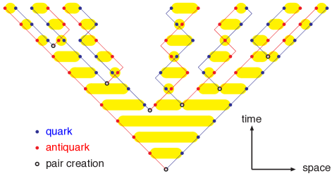
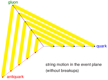
(a)                                                               (b)

Figure 1: (a) String breakup in a $\mathrm{q}\overline{\mathrm{q}}$ event. The points denote the location of quarks and antiquarks at snapshots in time, and the yellow regions the string pieces then stretched out between them. (b) String drawing in the plane of a $\mathrm{q}\overline{\mathrm{q}}\mathrm{g}$ event.

2.1 Hadronization

The Lund string model is based on the assumption of linear confinement, i.e. a string potential of $V=\kappa r$, where the string tension $\kappa\approx 1$ GeV/fm and $r$ is the separation between a colour triplet–antitriplet pair. For simplicity we may consider the process $\mathrm{e}^{+}\mathrm{e}^{-}\to\gamma^{*}/\mathrm{Z}^{0}\to\mathrm{q}\overline{\mathrm{q}}$, where the quark–antiquark pair moves out along the $\pm z$ axis, see Figure 1a. The linearity leads to a straightforward relationship between the energy–momentum and the space–time pictures:

$$\left|\frac{\mathrm{d}p_{z,\mathrm{q}/\overline{\mathrm{q}}}}{\mathrm{d}t}\right|=\left|\frac{\mathrm{d}p_{z,\mathrm{q}/\overline{\mathrm{q}}}}{\mathrm{d}z}\right|=\left|\frac{\mathrm{d}E_{\mathrm{q}/\overline{\mathrm{q}}}}{\mathrm{d}t}\right|=\left|\frac{\mathrm{d}E_{\mathrm{q}/\overline{\mathrm{q}}}}{\mathrm{d}z}\right|=\kappa~{}.$$ (1)

It is necessary to keep track of signs: as the $\mathrm{q}$-to-$\overline{\mathrm{q}}$ separation increases their energies decrease, with more and more of the energy instead stored in the intermediary string. At the maximal separation there would be no energy left for the quarks, and the string tension would then start to pull them together again, so that they would perform an oscillatory motion often referred to as a “yo-yo” motion.

If there is enough energy, the string between an original $\mathrm{q}_{0}\overline{\mathrm{q}}_{0}$ pair may break by producing new $\mathrm{q}_{i}\overline{\mathrm{q}}_{i}$ pairs, where the intermediate $\mathrm{q}_{i}$ ($\overline{\mathrm{q}}_{i}$) are pulled towards the $\overline{\mathrm{q}}_{0}$ ($\mathrm{q}_{0}$) end, such that the original colour field is screened. This way the system breaks up into a set of $n$ colour singlets $\mathrm{q}_{0}\overline{\mathrm{q}}_{1}-\mathrm{q}_{1}\overline{\mathrm{q}}_{2}-\mathrm{q}_{2}\overline{\mathrm{q}}_{3}-\ldots-\mathrm{q}_{n-1}\overline{\mathrm{q}}_{0}$, that we can associate with the primary hadrons. Each $\mathrm{q}_{i}\overline{\mathrm{q}}_{i}$ pair is produced with zero energy and momentum at its common vertex, since the string does not contain any local concentrations of energy. The energy and momentum of a hadron $\mathrm{h}_{i}=\mathrm{q}_{i}\overline{\mathrm{q}}_{i+1}$ therefore is provided by the string intermediate to the $\mathrm{q}_{i}\overline{\mathrm{q}}_{i}$ and $\mathrm{q}_{i+1}\overline{\mathrm{q}}_{i+1}$ breaks. This gives $E_{\mathrm{h}_{i}}=\kappa(z_{i}-z_{i+1})$ and $p_{z,\mathrm{h}_{i}}=\kappa(t_{i}-t_{i+1})$. Note that $z_{i}>z_{i+1}$ since $\mathrm{q}_{0}$ is moving in the $+z$ direction. If boosted to a frame where $t^{\prime}_{i}=t^{\prime}_{i+1}$, i.e. where the hadron is at rest, one obtains $m_{\mathrm{h}_{i}}=E^{\prime}_{\mathrm{h}_{i}}=\kappa(z^{\prime}_{i}-z^{\prime}_{i+1})$.

Unlike the intermediate vertices, the $\mathrm{q}_{0}\overline{\mathrm{q}}_{0}$ pair starts with non-vanishing energy at the origin. The equivalent vertex for the $\mathrm{q}_{0}$ instead is where it has lost its energy, which (in the massless approximation) occurs at $t=z=E_{\mathrm{q}_{0}}(t=0)/\kappa$. This vertex can be used as the starting point for a recursive procedure, where the location of each consecutive vertex can be reconstructed from the $E$ and $p_{z}$ of the intermediate hadron. Knowing the momenta of all hadrons it is therefore possible to reconstruct all $\mathrm{q}_{i}\overline{\mathrm{q}}_{i}$ production vertices, or the other way around. Hadrons do not have a unique definition of a production “vertex”, being extended objects, but a convenient choice is the average of the $\mathrm{q}_{i}\overline{\mathrm{q}}_{i}$ ones on either side of it [20]. Alternatives include an early or late choice, where the backward or forward light cones of the two $\mathrm{q}_{i}\overline{\mathrm{q}}_{i}$ vertices cross.

Several issues have here been swept under the carpet, since they do not directly affect the key relationship between the energy–momentum and the space–time pictures. One issue is that quarks with non-vanishing mass or $p_{\perp}$ should move along hyperbolae $E^{2}-p_{z}^{2}=m^{2}+p_{\perp}^{2}=m_{\perp}^{2}$. When produced inside a string they have to tunnel out a distance before they can end up on mass shell. This tunnelling process gives a suppression of heavier quarks, like $\mathrm{s}$ relative to $\mathrm{u}$ and $\mathrm{d}$ ones, and an (approximately) Gaussian distribution of the transverse momenta. Effective equivalent massless-case production vertices can be defined, e.g. by replacing $m$ by $m_{\perp}$ in relations between $E$ and $p_{z}$. Another issue is that the above notation only allows for meson production. Baryons can be introduced e.g. by considering diquark–antidiquark pair production, where a diquark is a colour antitriplet and thus can replace an antiquark in the flavour chain.

Having simultaneous knowledge of both the energy–momentum and the space–time picture of hadron production violates the Heisenberg uncertainty relations. In this sense the string model should be viewed as a semiclassical one, and there is no perfect way around that. Smearing factors will be introduced to largely remove the tension for the transverse degrees of freedom, and somewhat reduce it for the other ones. Either way, this semiclassical model does not introduce any clear systematic biases. Hence, there is no big problem in practice, since we are interested in average effects obtained by Monte Carlo sampling over a wide range of possible early histories.

The real practical hurdle is to go on from a simple straight string to a larger string system. Consider e.g. $\mathrm{e}^{+}\mathrm{e}^{-}\to\gamma^{*}/\mathrm{Z}^{0}\to\mathrm{q}\overline{\mathrm{q}}\mathrm{g}$. In the limit where the number of colours is large, the $N_{C}\to\infty$ approximation [33], a string will be stretched from the colour of the $\mathrm{q}$ to the anticolour of the $\mathrm{g}$, and then on from the colour of the $\mathrm{g}$ to the anticolour of the $\overline{\mathrm{q}}$, Fig. 1b. To first approximation the two string pieces each could be viewed as a boosted copy of a simple $\mathrm{q}\overline{\mathrm{q}}$ system. The problems arise around the gluon kink, as follows. We already noted that a $\mathrm{q}/\overline{\mathrm{q}}$ turns around when it has lost its energy. When the same thing happens for a gluon, however, it is instead replaced by a new expanding string region made out of inflowing momentum from the $\mathrm{q}$ and $\overline{\mathrm{q}}$. Therefore there are actually three string regions in which breaks can occur, and the third one is especially important in the limit of a low-energy gluon. Note that QCD favours the emission of soft gluons, and that additionally a gluon is pulling out two string pieces and therefore loses energy twice as fast as a quark, so such third regions contribute a fair fraction of all hadron production. For systems with more than one intermediate gluon the string motion becomes even more complicated.

A framework to handle energy and momentum sharing in such complicated topologies was developed in Ref. [34], and was then extended to reconstruct matching space–time production vertices in [20]. (An earlier extension in [35] included several of the same main features, but could not handle as complicated systems as required for LHC applications.) Again it can be described as a recursive procedure, starting from one end of the string system, but now with additional rules how to pass from one string region to the next. The reader is referred to Ref. [20] for details.

In addition to the main group of open strings stretched between $\mathrm{q}\overline{\mathrm{q}}$ endpoints, there are two other common string topologies. One is a closed gluon loop, which can be viewed as an open string (with at least one intermediate gluon) where the $\mathrm{q}$ and $\overline{\mathrm{q}}$ endpoints are fused into a single gluon, which closes the colour flow. Once an initial $\mathrm{q}_{0}\overline{\mathrm{q}}_{0}$ breakup has been picked somewhere along the string, at random (within given rules), the further handling devolves back into the open string framework. The other is the junction topology, represented by three quarks moving out in a different directions, each pulling out a string behind itself. These strings meet at a common junction vertex, to form a Y-shaped topology. The junction moves by the net pull of the string, and is at rest only in a frame where the opening angle between each quark pair is $120^{\circ}$. Also in this case there may be gluons on the string between a quark and the junction. Each of the three legs may be hadronized according to the same basic rules as above, with some special care needed where they meet at the junction, around which a baryon is formed to carry the net baryon number of the system.

There is one further aspect added to the framework presented so far. For the energy–momentum picture in a $\mathrm{q}\overline{\mathrm{q}}$ system we started out with a pure two-dimensional representation in $(E,p_{z})$ space, but then added random Gaussian $p_{\perp}$ kicks motivated by the tunnelling mechanism. Alternatively we could have motivated such fluctuations by the uncertainty relationship: a string could be expected to have a radius roughly $\sqrt{2/3}$ that of the proton, since if $r_{\mathrm{p}}^{2}=\langle x^{2}+y^{2}+z^{2}\rangle$ then $\langle x^{2}+y^{2}\rangle=(2/3)r_{\mathrm{p}}^{2}$. Either argument gives $p_{\perp}$ kicks of the order 0.3 GeV for each $\mathrm{q}_{i}\overline{\mathrm{q}}_{i}$ pair, consistent with data. By contrast, the basic machinery sets all $\mathrm{q}_{i}\overline{\mathrm{q}}_{i}$ production vertices to have $x=y=0$, which gives an unreasonably perfect lineup of the hadrons. For the studies in [20] we therefore introduced a Gaussian $(x,y)$ smearing with a width according to the expressions above, and will continue to do so. By the additional smearing to be introduced in the next section, which partially might overlap, some reduction of the width would be motivated, however.

Unfortunately, complications may arise in multiparton systems, notably for those hadrons that have their two defining $\mathrm{q}_{i}\overline{\mathrm{q}}_{i}$ vertices in two different string regions, meaning there is no unique separation between transverse and longitudinal degrees of freedom. Occasionally this may give unreasonably large positive or negative $\tau^{2}=t^{2}-x^{2}-y^{2}-z^{2}$. A few safety checks have been introduced to catch and correct such mishaps as well as possible.

2.2 Multiparton interaction vertices

The framework described above assumes that all partons start out from the same space–time production vertex, as would be the case e.g. in $\mathrm{e}^{+}\mathrm{e}^{-}\to\mathrm{Z}^{0}\to\mathrm{q}\overline{\mathrm{q}}$. In $\mathrm{p}\mathrm{p}$ the colliding hadrons are extended objects, however. The Lorentz-contracted hadrons pass through each other at a fairly well-defined time, conventionally $t=0$, but over a transverse region of hadronic sizes. In the overlap region several parton-parton interactions can occur, as described by the MPI framework in Pythia [17, 18].

The probability for an interaction at a given transverse coordinate $(x,y)$ can be assumed related to the time-integrated overlap of the parton densities of the colliding hadrons in that area element. Let the partons be described by a Lorentz contracted probability distribution $P_{\mathrm{LC}}(x,y,z)$, which in its rest frame reduces to a spherically symmetric $P(r)$ with $r^{2}=x^{2}+y^{2}+z^{2}$. Setting the two incoming beam particles $A$ and $B$ to move along the $z$ axis with velocity $\pm v$, separated by $\pm b/2$ in the $x$ direction, where $b$ is the impact parameter, this overlap (“eikonal”) reads

$$\mathcal{O}(x,y;b) \propto \int\!\int P_{\mathrm{LC},A}\left(x-\frac{b}{2},y,z-vt\right)\,P_{\mathrm{LC},B}\left(x+\frac{b}{2},y,z+vt\right)\,\mathrm{d}z\,\mathrm{d}t$$ (2)

$$\propto \int P_{A}\left(x-\frac{b}{2},y,z_{A}\right)\,\mathrm{d}z_{A}\;\int P_{B}\left(x-\frac{b}{2},y,z_{B}\right)\,\mathrm{d}z_{B}~{},$$

the latter by suitable variable transformation. The answer can be further simplified in case of a Gaussian distribution $P(r)\propto\exp(-r^{2}/r_{0}^{2})$:

$$\mathcal{O}(x,y;b) \propto \int\exp\left(\frac{(x-b/2)^{2}+y^{2}+z_{A}^{2})}{r_{0}^{2}}\right)\,\mathrm{d}z_{A}\;\int\exp\left(\frac{(x+b/2)^{2}+y^{2}+z_{B}^{2})}{r_{0}^{2}}\right)\,\mathrm{d}z_{B}$$ (3)

$$\propto \exp\left(-\frac{2r_{\perp}^{2}}{r_{0}^{2}}\right)\,\exp\left(-\frac{\mathrm{b}^{2}}{2r_{0}^{2}}\right)~{},$$

where $r_{\perp}^{2}=x^{2}+y^{2}$. That is, for a Gaussian proton the overlap region is an azimuthally symmetric Gaussian, with no memory of the collision plane, and the total overlap is a Gaussian in $b$. The $r_{0}$ parameter can be approximately related to the proton radius $r_{\mathrm{p}}$ by $\langle r^{2}\rangle=\langle x^{2}+y^{2}+z^{2}\rangle=3r_{0}^{2}/2=r_{\mathrm{p}}^{2}$. The default in Pythia is a constant proton radius value $r_{\mathrm{p}}\approx 0.85$ fm for the distribution of partons. With increasing energy, and a related increase in the number of MPIs per collision, the effective edge of interacting partons is pushed outwards and thus collision cross sections can go up.

The Gaussian is a very special case, however. In general, the collision region will be elongated either out of or in to the collision plane. The former typically occurs for a distribution with a sharper proton edge, e.g. a uniform ball, $P(r)\propto\Theta(r_{0}-r)$, where $\Theta$ is the step function, which gives rise to the almond-shaped collision region so often depicted for heavy-ion collisions. The latter shape instead occurs for distributions with a less pronounced edge, such as an exponential, $P(r)\propto\exp(-r/r_{0})$.

In the Pythia MPI machinery the overlap distribution $\mathcal{O}(b)=\int\!\int\mathcal{O}(x,y;b)\,\mathrm{d}x\,\mathrm{d}y$ can be chosen and tuned according to a few different forms. The current default is $\mathcal{O}(b)\propto\exp((b/b_{0})^{p})$ with $p=1.85$, i.e. close to but not quite Gaussian. A similar shape and tune is obtained with a double Gaussian $P(r)$, where a smaller-radius second Gaussian can be viewed as representing hot spots inside the proton. In both cases a stronger-than-Gaussian peaking of $\mathcal{O}(b)$ at $b=0$ is required to get a sufficiently long tail out to largest charged multiplicities in LHC and Tevatron minimum-bias events.

The $P(r)$ and $\mathcal{O}(b)$ distributions as described so far are likely to be significant simplifications, however. If one views the evolution from a simple original parton configuration via initial-state cascades into a set of interacting partons, then there are likely to arise complicated patterns and correlations. One such framework is presented in Ref. [36], where an implementation of Mueller’s dipole model [37, 38] for the two colliding hadrons are used to assign MPI production vertices. These then turn out to give clearly non-isotropic distributions. In the future the relevant code for these assignments will be made available, but using it comes at a cost in terms of a considerably slower event generation.

For now, we have therefore settled for a simplified framework with enough flexibility for our purposes. In it the MPIs locations by default are selected according to the Gaussian $\exp(-2r_{\perp}^{2}/r_{0}^{2})$, but optionally this can be modified in either of two ways. Either the $x$ coordinates are scaled by a factor $r_{\epsilon}$ and the $y$ ones by $1/r_{\epsilon}$, or else the Gaussian is multiplied by a $\varphi$ modulation factor

$$\frac{\mathrm{d}N}{\mathrm{d}\varphi}\propto 1+\epsilon\cos(2\varphi)~{}.$$ (4)

Here $r_{\epsilon}>1$ or $\epsilon>0$ means an enhancement in the collision plane and $r_{\epsilon}<1$ or $\epsilon<0$ out of it. Asymmetries in the spatial distribution also arise from the Monte Carlo sampling of a finite number of MPIs, and these may be even more important.

This machinery is used to select the $(x,y)$ coordinates of the MPI vertices at $t=z=0$. Only a fraction of the full beam-particle momentum is carried away by the MPIs, leaving behind one or more beam remnants [39]. These are initially distributed according to the basic $\exp(-r_{\perp}^{2}/r_{0}^{2})$ shape around the center of the respective beam. By the random fluctuations, and by the interacting partons primarily being selected on the side leaning towards the other beam particle, the “center of gravity” will not be located at the $x=\pm b/2,y=0$ positions originally assumed. All the beam remnants will therefore be shifted so as to ensure that the energy-weighted sum of colliding and remnant parton locations is where it should be. As a small improvement on a uniform shift, remnants located closer to the other remnant are shifted more, so as to deplete the overlap region more. This is achieved by assigning each remnant a weight

$$\left(1+\frac{b}{r_{\mathrm{p}}}\exp\left(\frac{\pm x}{r_{\mathrm{p}}}\right)\right)^{-1}$$ (5)

proportional to its eventual shift, where $x$ is relative to the respective beam center with the other beam displaced $\mp b$ in the $x$ direction. Shifts are capped to be at most a proton radius, so as to avoid extreme spatial configurations, at the expense of a perfectly aligned center of gravity.

Not all hadronizing partons are created in the collision moment $t=0$. Initial-state radiation (ISR) implies that some partons have branched off already before this, and final-state radiation (FSR) that others do it afterwards. These partons then can travel some distance out before hadronization sets in, thereby further complicating the space–time picture, even if the average time of parton showers typically is a factor of five below that of string fragmentation [20]. We will not trace the full shower evolution, but instead include a smearing of the transverse location in the collision plane that a parton points back to. Specifically, a radiated parton is assigned a location at $t=0$ that is smeared by $\Delta r_{\perp}$ relative to its mother parton according to a two-dimensional Gaussian with a width inversely proportional to its $p_{\perp}$. The constant of proportionality can be set freely, but should obviously be such that $\Delta r_{\perp}\,p_{\perp}\sim\hbar$. So as not to obtain unreasonable $\Delta r_{\perp}$ shifts, the $p_{\perp}$ is set to be at least 0.5 GeV in this context, comparable to the cut-off scale of the FSR showers. No attempt is made to preserve the center of gravity during these fluctuations.

The partons produced in various stages of the collision process (MPIs, ISR, FSR) are initially assigned colours according to the $N_{C}\to\infty$ approximation, such that different MPI systems are decoupled from each other. By the beam remnants, which have as one task to preserve total colour, these systems typically become connected with each other. Furthermore, colour reconnection (CR) is allowed to swap colours, partly to compensate for finite-$N_{C}$ effects, but mainly that it seems like nature prefers to reduce the total string length drawn out when two nearby strings overlap each other. When such effects have been taken into account, what remains to hadronize is one or more separate colour singlet systems of the character already described in Section 2.1.

There is one key difference, however, namely that the strings now can be stretched between partons that do not originate from the same vertex. Even in the simplest case, a $\mathrm{q}$ connected with a $\overline{\mathrm{q}}$ from a different MPI, there is a new situation not studied previously, where the vertex separation should be equivalent to a piece of string already at $t=0$. For the energy–momentum picture it is traditionally assumed that its effects are sufficiently small that they can be neglected. If the effects of a 1 fm $\approx$ 1 GeV special term is to be spread over many hadrons, then the net effect on each hardly would be noticeable.

For the space–time picture we do want to be more careful about the effects of the transverse size of the original source. The bulk of the effects determining the hadronic production vertices do come from the framework of Section 2.1, and therefore we will be satisfied if we can introduce a relevant amount of smearing on hadron production, without necessarily fully describe effects for the individual hadron. This is achieved as follows.

For a simple $\mathrm{q}\overline{\mathrm{q}}$ string, such as in Figure 1a, the relevant length of each hadron string piece is related to its energy. For a given hadron, define $E_{\mathrm{h}\mathrm{q}}$ ($E_{\mathrm{h}\overline{\mathrm{q}}}$) as half the energy of the hadron plus the full energy of all hadrons lying between it and the $\mathrm{q}$ ($\overline{\mathrm{q}}$) end, and use this as a measure of how closely associated a hadron is with the respective endpoint. Also let $\mathbf{r}_{\perp\mathrm{q}}$ ($\mathbf{r}_{\perp\overline{\mathrm{q}}}$) be the (anti)quark transverse production coordinates. Then define the hadron production vertex offset to be

$$\Delta\mathbf{r}_{\perp\mathrm{h}}=\frac{E_{\mathrm{h}\overline{\mathrm{q}}}\,\mathbf{r}_{\perp\mathrm{q}}+E_{\mathrm{h}\mathrm{q}}\,\mathbf{r}_{\perp\overline{\mathrm{q}}}}{E_{\mathrm{h}\mathrm{q}}+E_{\mathrm{h}\overline{\mathrm{q}}}}=\frac{(E_{\mathrm{tot}}-E_{\mathrm{h}\mathrm{q}})\,\mathbf{r}_{\perp\mathrm{q}}+E_{\mathrm{h}\mathrm{q}}\,\mathbf{r}_{\perp\overline{\mathrm{q}}}}{E_{\mathrm{tot}}}~{},$$ (6)

relative to what a string motion started at the origin would have given.

This procedure is then generalized to more complicated string topologies. In a $\mathrm{q}-\mathrm{g}_{1}-\mathrm{g}_{2}-\ldots-\overline{\mathrm{q}}$ string, one may define $E_{\mathrm{h}\mathrm{q}}$ as above. If $E_{\mathrm{h}\mathrm{q}}<E_{\mathrm{q}}+E_{\mathrm{g}_{1}}/2$ the hadron is viewed as produced between the $\mathrm{q}$ and $\mathrm{g}_{1}$, and the offset can be found as above, only with $E_{\overline{\mathrm{q}}}$ replaced by $E_{\mathrm{g}_{1}}/2$. If instead $E_{\mathrm{q}}+E_{\mathrm{g}_{1}}/2<E_{\mathrm{h}\mathrm{q}}<E_{\mathrm{q}}+E_{\mathrm{g}_{1}}+E_{\mathrm{g}_{2}}/2$ then the excess energy $E_{\mathrm{h}\mathrm{q}}-E_{\mathrm{q}}-E_{\mathrm{g}_{1}}/2$ determines the admixture of $\mathbf{r}_{\perp\mathrm{g}_{1}}$ and $\mathbf{r}_{\perp\mathrm{g}_{2}}$, and so on, stepping through region after region, for hadron after hadron, until the $\overline{\mathrm{q}}$ end is reached. For junction topologies the same kind of approach can be used to iterate from each leg towards the central junction. The two lowest-energy legs are considered first, and an $\mathbf{r}_{\perp}$ towards which the third string is iterated is formed by the relative unused energy fractions of the first two. That way a junction baryon can receive contributions from all three legs.

There are two obvious shortcomings. Firstly, the approach does not take into account the higher regions, handled in the complete string motion, e.g. made up out of $\mathrm{q}$ and $\mathrm{g}_{2}$ momentum, where the hadron offset could be a more complex combination of three different parton offsets. Secondly the sharing according to energy is not Lorentz covariant. Nevertheless, we believe this approach to provide a sensible approximation to the smearing effects one may expect. There is also a third, less obvious problem, namely what to do with closed gluon loops. There the hadronization is begun at a random point, where the location of this point currently is not stored anywhere. The algorithm as presented so far will start at another point and therefore give a mismatch. We have not considered this a big issue for now, since the default CR algorithm will dissolve almost all such closed loops, and again the key issue is to provide some relevant amount of smearing without attaching too deep a meaning to each separate correction to the dominant hadronization picture.

2.3 The space–time picture of hadronic rescattering

By the procedure outlined so far, each primary produced hadron has been assigned a production vertex $x_{0}=(t_{0},\mathbf{x}_{0})$ and a four-momentum $p=(E,\mathbf{p})$. The latter defines its continued motion along straight trajectories $\mathbf{x}(t)=\mathbf{x}_{0}+(t-t_{0})\,\mathbf{p}/m$. Consider now two particles produced at $x_{1}$ and $x_{2}$ with momenta $p_{1}$ and $p_{2}$. Our objective is to determine whether these particles will scatter and, if so, when and where. To this end, the potential collision is studied in the center-of-momentum frame of the two particles, with motion along the $\pm z$ direction, i.e.

$$\begin{split}p_{1}&=(E_{1},0,0,p)~{},\\ p_{2}&=(E_{2},0,0,-p)~{}.\end{split}$$ (7)

If they are not produced at the same time, the position of the earlier particle is offset to the creation time of the later particle. Particles moving away from each other already at this common time, i.e. with $z_{1}>z_{2}$, are assumed unable to scatter.

Otherwise, the probability $P$ of an interaction is a function of the impact parameter $b$, the center-of-mass energy, and the two particle species. There is no solid theory for the $b$ dependence of $P$, so we will consider two different shapes. The default model is a Gaussian dependency,

$$P(b)=P_{0}e^{-b^{2}/b_{0}^{2}},$$ (8)

where $P_{0}$ is referred to as the opacity, a free parameter that is 0.75 by default, and the characteristic length scale is

$$b_{0}=\sqrt{\frac{\sigma}{P_{0}\pi}}~{},$$ (9)

where $\sigma$ is the cross section. It is assumed that the only dependency on the energy and the particle species is through $\sigma$, which will be discussed in great detail in Section 3. Typical values of $b_{0}$ are around 1-2 fm for the most common processes. An alternative model is a grey disk with interaction probability

$$P(b)=P_{0}\,\Theta(b-b_{0}),$$ (10)

where $\Theta$ is the Heaviside step function. The $P_{0}=1$ case gives the often-used black disk limit. In both these cases, the parameter $b_{0}$ is chosen so that

$$\int\limits_{0}^{\infty}2\pi b\,P(b)\,\mathrm{d}b=\sigma~{}.$$ (11)

This normalization ensures that if $b$ is chosen uniformly on a large disk, the total probability of an interaction is the same for both models. In reality, with a finite effective region, one may expect the Gaussian shape to give fewer scatterings.

If it is determined that the particles will interact, the interaction time is defined as the time of closest approach in the rest frame. The spatial component of the interaction vertex depends on the character of the collision. Elastic and diffractive processes can be viewed as $t$-channel exchanges of a pomeron (or reggeon), and then it is reasonable to let each particle continue out from its respective location at the interaction time. For other processes, where either an intermediate $s$-channel resonance is formed or strings are stretched between the remnants of the two incoming hadrons, an effective common interaction vertex is defined as the average of the two hadron locations at the interaction time. In cases where strings are created, be it by $s$-channel processes or by diffraction, the hadronization starts around this vertex and is described in space–time as already outlined. This means an effective delay before the new hadrons are formed and can begin to interact. For the other processes, such as elastic scattering or an intermediate resonance decay, there is the option to have effective formation times before new interactions are allowed. One reason for why one would want this is that it takes some time for the new hadrons to break free from the volume formerly occupied by the mothers and form their own new (spatial) wave functions.

In actual events with many hadrons, each hadron pair is checked to see if it fulfils the interaction criteria and, if it does, the interaction time for that pair (in the CM frame of the event) is recorded in a time-ordered list. During rescattering, unstable particles can decay, with the fastest-decaying ones having lifetimes comparable to the timescales of rescattering. For these particles, an invariant lifetime $\tau$ is picked at random according to an exponential $\exp(-\tau/\tau_{0})$, where $\tau_{0}=1/\Gamma$ is the inverse of the width. This is done for each short-lived hadron, and the resulting decay times are inserted into the same list. Then the scattering or decay that is first in time order is simulated unless the particles involved have already interacted/decayed. This produces new hadrons that are checked for rescatterings or decays, and any such are inserted into the time-ordered list. This process is repeated until there are no more potential interactions.

There are some obvious limitations to the approach as outlined so far:

Firstly, the procedure is not Lorentz invariant, since the time-ordering of interactions is defined on the lab frame of the full collision, i.e. the CM frame for LHC events. We do not expect this to be a major issue: even if the time ordering would change depending on the frame chosen, it would not matter in choosing between two potential interactions with a spacelike separation, and only for a fraction of those with a timelike one. This has been studied and confirmed within existing rescattering approaches [28, 40, 29]. We will also present a check in Section 4.4, where we confirm that the effect on observable quantities is negligible. More consistent time orderings have been proposed [41, 42], but are nontrivial to implement and have not been considered here.

Secondly, currently only collisions between two incoming hadrons are considered, even though in a dense environment one would also expect collisions involving three or more hadrons. If one considers a closed system in thermal equilibrium, where $2\to n$ processes are allowed, indeed $n\to 2$ at commensurate rates would be a natural ingredient to maintain that balance. The system is rapidly expanding in $\mathrm{p}\mathrm{p}$ collisions, so for our current studies it should not be a big issue. One place where it could make a difference is in baryon rates, where pair annihilation outweighs pair creation within the current setup. In the future $3\to n$ collisions could be identified by isolating cases where a hadron has two very closely separated potential $2\to n$ interactions, which then could be joined into one. This would also introduce an alternative argument for a formation time, as the borderline between separated and joined processes.

Thirdly, introducing rescattering will change the shape of events, which of course is the point of the exercise, but it also affects distributions we do not want to change. One example, related to the second limitation above, is that the charged multiplicity will increase, which has to be compensated by a tuning of other parameters. In this article only a simple retune is made specifically for $\mathrm{p}\mathrm{p}$. More properly one should go back to $\mathrm{e}^{+}\mathrm{e}^{-}$ annihilation events and retune the fragmentation of a simple string there, with rescattering effects included, before proceeding to $\mathrm{p}\mathrm{p}$. In $\mathrm{e}^{+}\mathrm{e}^{-}\to\mathrm{Z}^{0}\to\mathrm{q}\overline{\mathrm{q}}$ events, however, the bulk of rescattering should be related to nearest neighbours in rank, i.e. in order along the string. So, if such rescatterings are not simulated, then fragmentation parameters should not have to be changed significantly. A shortcut to avoid a bigger retune therefore is to forbid nearest-rank neighbours from rescattering also in $\mathrm{p}\mathrm{p}$ events, and this is one model variation we will consider.

Fourthly, all possible subprocesses are assumed to share the same impact-parameter profile. In a more detailed modelling the $t$-channel elastic and diffractive processes should be more peripheral than the rest, and display an approximately inverse relationship between the $t$ and $b$ values.

Finally, the model only considers the effect of hadrons colliding with hadrons, not those of strings colliding/overlapping with each other or with hadrons. The former is actively being studied within Pythia, as a shoving/repulsion of strings [15, 43]. Both shove and rescattering act to correlate the spatial location of strings/hadrons with a net push outwards, giving rise to a radial flow. In reality the two could be combined, with shove acting before hadronization and rescattering after. The two effects do not add linearly, however, since an early shove leads to a more dilute system of strings and primary hadrons, and thereby less rescattering. Thus it will become a nontrivial task to distinguish the effects of the two possible phenomena, not made any simpler if also string–hadron interactions were to be included in the mix.

3 The hadronic rescattering model

A crucial input for deciding whether a scattering can occur is the total cross section. Once a potential scattering is selected, it also becomes necessary to subdivide the total cross section into a sum of partial cross sections, one for each possible process, as these are used to represent relative frequencies for each process to occur. In this section, we discuss the possible processes we have implemented in our framework, including how their partial cross sections are calculated, and how those processes are simulated.

As we will see, a staggering amount of details enter in such a description, owing to the multitude of incoming particle combinations and collision processes. To wit, not only “long-lived” hadrons can collide, i.e. $\pi$, $\mathrm{K}$, $\eta$, $\eta^{\prime}$, $p$, $n$, $\Lambda$, $\Sigma$, $\Xi$, $\Omega$, and their antiparticles, but also a wide selection of short-lived hadrons, starting with $\rho$, $\mathrm{K}^{*}$, $\omega$, $\phi$, $\Delta$, $\Sigma^{*}$ and $\Xi^{*}$. The possible processes that can occur depend heavily on the particle types involved. In our model, the following types of processes are available:

• Elastic interactions are ones where the particles do not change species, i.e. $AB\to AB$. In our implementation, these are considered different from elastic scattering through a resonance, e.g. $\pi^{+}\pi^{-}\to\rho^{0}\to\pi^{+}\pi^{-}$ (in reality there are likely to be interference terms that make this separation ambiguous). In experiments, usually all $AB\to AB$ events are called elastic because it is not possible to tell which underlying mechanism was involved. Therefore, when comparing with data for elastic cross sections, we do include contributions from resonance formation.

• Resonance formation typically can be written as $AB\to R\to CD$, where $R$ is the intermediate resonance. This can only occur when one or both of $A$ and $B$ are mesons. It is the resonances that drive rapid and large cross-section variations with energy, since each (well separated) resonance should induce a Breit-Wigner peak.

• Annihilation is specifically aimed at baryon–antibaryon collisions where the baryon numbers cancel out and gives a mesonic final state. This is assumed to require the annihilation of at least one $\mathrm{q}\overline{\mathrm{q}}$ pair. This is reminiscent of what happens in resonance formation, but there the final state is a resonance particle, while annihilation forms strings between the outgoing quarks.

• Diffraction of two kinds are modelled here: single $AB\to XB$ or $AB\to AX$ and double $AB\to X_{1}X_{2}$. Here $X$ represents a massive excited state of the respective incoming hadron, and there is no net colour exchange between the two sides of the event.

• Excitation can be viewed as the low-mass limit of diffraction, where either one or both incoming hadrons are excited to a related higher resonance. It can be written as $AB\to A^{*}B$, $AB\to AB^{*}$ or $AB\to A^{*}B^{*}$. Here $A^{*}$ and $\mathrm{B}^{*}$ are modelled with Breit-Wigners, as opposed to the smooth mass spectra of the $X$ diffractive states. In our description, this has only been implemented in nucleon-nucleon interactions.

• Nondiffractive topologies are assumed to correspond to a net colour exchange between the incoming hadrons, such that colour strings are stretched out between them after the interaction.

All total and partial cross sections have a nontrivial energy dependence. Whereas we have made an effort to cover a fair amount of detail, it is not feasible to give all processes full attention in the first release of this framework, not even in the proportionately few cases where experimental data exist. Our hope is that since rescatterings will not be observable on an individual basis and instead the average effects they induce is what will be of interest, we can live with imperfections here and there so long as they do not generate non-negligible systematic biases. Refinements could be introduced over time without affecting the rescattering machinery as such. In Section 4.5 we will study the rates of different particle types participating in rescattering and at which energies most interactions occur, giving an indication of which cross sections are the most important for future refinement.

In the continued discussion, some common simplifications should be noted.

• Cross sections are invariant when all particles are replaced by their antiparticles. Whenever we talk about any particular cross section for two particles, it is always implicit that the exact same procedure is used to calculate the cross section for their antiparticles.

• Many measured cross sections approximately scale in accordance with the Additive Quark Model (AQM) [44, 45], i.e. like the product of the number of valence quarks in the two incoming hadrons. The contribution of heavier quarks is scaled down relative to that of a $\mathrm{u}$ or $\mathrm{d}$ quark, presumably by mass effects giving a narrower wave function. Assuming that quarks contribute inversely proportional to their constituent masses, this gives an effective number of interacting quarks in a hadron of approximately

  $$n_{\mathrm{q},\mathrm{AQM}}=n_{\mathrm{u}}+n_{\mathrm{d}}+0.6\,n_{\mathrm{s}}+0.2\,n_{\mathrm{c}}+0.07\,n_{\mathrm{b}}~{}.$$ (12)

  For lack of alternatives, many unmeasured cross sections are assumed to scale in proportion to this.

• The neutral Kaon system is nontrivial, with strong interactions described by the $\mathrm{K}^{0}/\overline{\mathrm{K}}^{0}$ states and weak decays by the $\mathrm{K}^{0}_{\mathrm{S}}/\mathrm{K}^{0}_{\mathrm{L}}$ ones. The oscillation time is of the order of the $\mathrm{K}^{0}_{\mathrm{S}}$ lifetime, far above the rescattering scales of interest in this article. Therefore an intermediate “decay” invariant time of $10^{9}$ fm has been introduced for $\mathrm{K}^{0}/\overline{\mathrm{K}}^{0}\to\mathrm{K}^{0}_{\mathrm{S}}/\mathrm{K}^{0}_{\mathrm{L}}$, well above hadronization scales but also well below decay ones. While the bulk of Kaon production is into the strong eigenstates, a fraction is into the weak ones, such as $\phi\to\mathrm{K}^{0}_{\mathrm{S}}\,\mathrm{K}^{0}_{\mathrm{L}}$. Cross sections for $\mathrm{K}_{S}^{0}/\mathrm{K}_{\mathrm{L}}^{0}$ with a hadron are given by the mean of the cross section for $\mathrm{K}^{0}$ and $\overline{\mathrm{K}}^{0}$ with that hadron. When the collision occurs, the $\mathrm{K}_{\mathrm{S,L}}$ is converted into either $\mathrm{K}^{0}$ or $\overline{\mathrm{K}}^{0}$, where the probability for each is proportional to the total cross section for the interaction with that particle.

Finally, keep in mind that we here concern ourselves with cross sections for collisions at low CM energies, with most rescatterings occurring below 2 GeV, and very few above 5 GeV, as we will see.

3.1 Total cross sections

The total cross section is needed by the rescattering algorithm to determine how close two hadrons need to be to interact. In the rescattering algorithm, each hadron pair (including the products of rescatterings) is checked for potential interactions, and thus naively $\mathcal{O}(n_{\mathrm{primary}}^{2})$ total cross sections must be calculated. Quick checks that can exclude a fair fraction of all pairs at an early stage are essential to keep time consumption at a manageable level. In particular, we have made an effort to ensure that total cross sections can be calculated efficiently, and that partial cross sections are only calculated for a hadron pair when it has been determined that they should interact.

A brief summary of total cross sections is provided in Table 1. Figure 2 shows the total and elastic cross sections for some important processes where PDG data is available [46].

Case	Method
$\mathrm{N}\mathrm{N}$, $<5$ GeV	Fit to data
$\mathrm{N}\mathrm{N}$, $>5$ GeV	$HPR_{1}R_{2}$ parameterization
Other $\mathrm{B}\mathrm{B}$	AQM (UrQMD) parameterization
$\mathrm{p}\overline{\mathrm{p}}$, $<5$ GeV	Ad hoc parameterization
$\mathrm{p}\overline{\mathrm{p}}$, $>5$ GeV	$HPR_{1}R_{2}$ parameterization
Other $\mathrm{B}\overline{\mathrm{B}}$	AQM rescaling of $\mathrm{p}\overline{\mathrm{p}}$
$\pi\pi$ and $\mathrm{K}\pi$	Parameterization based on [47, 48] and [49]
$\mathrm{N}\mathrm{K}^{-},\mathrm{N}\overline{\mathrm{K}}^{0}$	Resonances + ad hoc parameterization
$\mathrm{N}\mathrm{K}^{+},\mathrm{N}\mathrm{K}^{0}$	Ad hoc parameterization
$\mathrm{M}\mathrm{B}/\mathrm{M}\mathrm{M}$ with resonances	Resonances + elastic
Other $\mathrm{M}\mathrm{B}/\mathrm{M}\mathrm{M}$	$HPR_{1}R_{2}$ if available, otherwise AQM

Table 1: Summary of total cross section descriptions. Here, $\mathrm{N}$ is used to denote a nucleon ($\mathrm{p}$ or $\mathrm{n}$), $\mathrm{B}$ a baryon and $\mathrm{M}$ a meson.

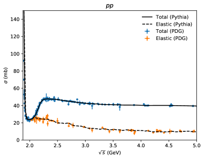
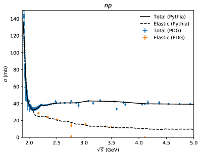
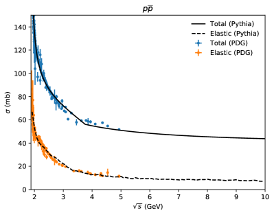
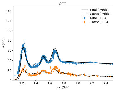
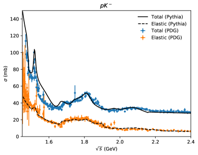
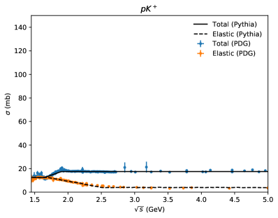
Figure 2: Total and elastic cross sections for some important processes. The elastic cross sections for $\mathrm{p}\pi^{-}$ and $\mathrm{p}\mathrm{K}^{-}$ include elastic scattering through a resonance, $AB\to R\to AB$, which notably do not correspond to the elastic cross sections calculated in Section 3.2.

3.1.1 Baryon-baryon

For $\mathrm{N}\mathrm{N}$ collisions below 5 GeV, the total cross section is found by an interpolation of experimental data [46]. The $\mathrm{n}\mathrm{n}$ cross section is taken to be the same as the $\mathrm{p}\mathrm{p}$ one. Above 5 GeV, the cross section is found using the $HPR_{1}R_{2}$ parameterization [46],

$$\sigma_{\mathrm{tot}}=P+H\log^{2}\left(\frac{s}{s_{0}}\right)+R_{1}\left(\frac{s}{s_{0}}\right)^{\eta_{1}}+R_{2}\left(\frac{s}{s_{0}}\right)^{\eta_{2}}~{},$$ (13)

where:

• $P$, $R_{1}$ and $R_{2}$ depend on the specific particle species, as shown in Table 2.

• $s_{0}$ depends on the masses of $A$ and $B$ and is given by $(m_{A}+m_{B}+M)^{2}$, where $M=2.1206$ GeV is a constant.

• $H=\pi(\hbar c)^{2}/M^{2}=0.2720$ mb, $\eta_{1}=0.4473$ and $\eta_{2}=0.5486$ are constants.

In other baryon–baryon cases, the cross section is found using the AQM ansatz as

$$\sigma_{\mathrm{AQM},AB}=(40~{}\mathrm{mb})\,\frac{n_{\mathrm{q},\mathrm{AQM},A}}{3}\,\frac{n_{\mathrm{q},\mathrm{AQM},B}}{3}~{}.$$ (14)

Process	$P$	$R_{1}$	$R_{2}$
$\mathrm{p}\mathrm{p}/\mathrm{n}\mathrm{n}$	34.41	13.07	-7.394
$\mathrm{p}\mathrm{n}$	34.71	12.52	6.66
$\overline{\mathrm{p}}\mathrm{p}$	34.41	13.07	7.394
$\mathrm{N}\pi^{\mp}$	18.75	9.56	$\pm$1.767
$\mathrm{p}\overline{\mathrm{K}}$	16.36	4.29	3.408
$\mathrm{n}\overline{\mathrm{K}}$	16.31	3.70	1.826

Table 2: Parameters for the $HPR_{1}R_{2}$ parameterization, for processes used in our rescattering framework. All numbers are in units of mb. $\mathrm{N}$ stands for either $\mathrm{p}$ or $\mathrm{n}$ and $\overline{\mathrm{K}}$ stands for either $\mathrm{K}^{-}$ or $\overline{\mathrm{K}}^{0}$.

3.1.2 Baryon-antibaryon

For $\mathrm{B}\overline{\mathrm{B}}$, we parameterize the cross section as a function of the absolute value of the center-of-mass momentum $p_{\mathrm{CM}}$ of the colliding hadrons. For $\mathrm{p}\overline{\mathrm{p}}$ below $p_{\mathrm{CM}}<6.5$ GeV, we use the UrQMD parameterization [28]:

$$\sigma_{\mathrm{tot}}(\mathrm{p}\overline{\mathrm{p}})=\begin{cases}271.6e^{-1.1\,p^{2}}~{},&p<0.3~{},\\ 75.0+43.1\,p^{-1}+2.6\,p^{-2}-3.9\,p~{},&0.3<p<6.5~{},\end{cases}$$ (15)

For $p_{\mathrm{CM}}>6.5$ GeV, we use $HPR_{1}R_{2}$. The boundary at 6.5 GeV has been chosen to give a smooth transition between the two regions, and is slightly different from the boundary at 5 GeV used by UrQMD. For all other baryon-antibaryon interactions, the total cross section is found using the same parameterization, but rescaling by an AQM factor,

$$\sigma_{\mathrm{tot}}(\mathrm{B}\overline{\mathrm{B}})=\frac{\sigma_{\mathrm{AQM},\mathrm{B}\overline{\mathrm{B}}}}{\sigma_{\mathrm{AQM},\mathrm{p}\overline{\mathrm{p}}}}\,\sigma_{\mathrm{tot}}(\mathrm{p}\overline{\mathrm{p}})~{},$$ (16)

where $\sigma_{\mathrm{AQM}}$ is given in eq. (14).

In some cases no quarks can annihilate, e.g. for $\Delta^{++}(\mathrm{u}\mathrm{u}\mathrm{u})+\overline{\Delta}^{+}(\overline{\mathrm{d}}\overline{\mathrm{d}}\overline{\mathrm{d}})$. In these cases, the annihilation cross section (see Section 3.4) is subtracted from the total one.

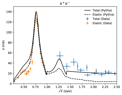
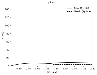
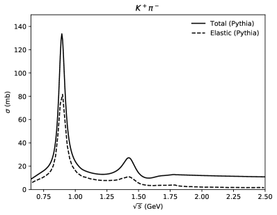
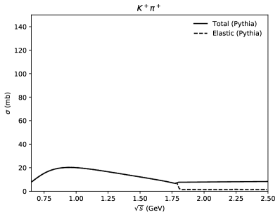
Figure 3: Total and elastic cross sections for $\pi\pi$ and $\mathrm{K}\pi$ interactions. We see that resonances exist for $\pi^{+}\pi^{-}$ and $\mathrm{K}^{+}\pi^{-}$, but not for $\pi^{+}\pi^{+}$ and $\mathrm{K}^{+}\pi^{+}$. The elastic cross sections include cross sections for elastic scattering through a resonance. For $\pi^{+}\pi^{-}$, the elastic data comes from [50, 51] and total data comes from [52, 53]. Note that in some theory calculations the concept of elastic is extended to related processes, e.g. $\pi^{+}\pi^{-}\to\pi^{0}\pi^{0}$ may count as part of a broader $\pi\pi\to\pi\pi$ “elastic” process. If we had taken that viewpoint, the elastic cross sections for $\pi^{+}\pi^{-}$ and $\mathrm{K}^{+}\pi^{-}$ would have equalled the total cross section at low energies.

3.1.3 Meson-hadron

The most common meson-meson interactions are $\pi\pi$ and $\mathrm{K}\pi$. In these two cases, the total cross sections are found using the calculations of Peláez et al. [47, 48, 49]. Below $1.42$ GeV for $\pi\pi$ and below $1.8$ GeV for $\mathrm{K}\pi$, values of the total cross sections have been tabulated and are found using interpolation, for the sake of efficiency. Above these thresholds, the cross section is parameterized as

$$\sigma_{\mathrm{tot}}(AB)=\frac{4\pi^{2}\left(\beta_{P}s+\beta_{\rho}s^{\alpha_{\rho}}+\beta_{2}s^{\alpha_{R2}}\right)}{\sqrt{(s-(m_{A}-m_{B})^{2})(s-(m_{A}+m_{B})^{2})}},$$ (17)

where, $\alpha_{\rho}=0.53$, $\alpha_{R2}=2\alpha_{\rho}-1=0.06$, and the $\beta$ parameters depend on the exact process as given in Table 3. Total and elastic cross sections for $\pi\pi$ and $\mathrm{K}\pi$ interactions are shown in Figure 3.

Case	$\beta_{P}$	$\beta_{\rho}$	$\beta_{2}$
$\pi^{\pm}\pi^{\mp}$	0.83	1.01	0.013
$\pi^{\pm}\pi^{0}$	0.83	0.267	-0.0267
$\pi^{0}\pi^{0}$	0.83	0.267	0.053
$\pi^{\pm}\pi^{\pm}$	0.83	-0.473	0.013
$\mathrm{K}\pi^{\pm},I=1/2$	6.9032	8.2126	0.0
$\mathrm{K}\pi^{0},I=1/2$	3.4516	4.1063	0.0
$\mathrm{K}\pi,I=3/2$	10.3548	-5.76786	0.0

Table 3: Parameter values for the $\pi\pi$ and $\mathrm{K}\pi$ cross sections, as used in eq. (17). In the case of $\mathrm{K}\pi$, $I$ refers to the sum of the third isospin components for the incoming particles. The two $I=1/2$ cases are equivalent, except for Clebsch-Gordan coefficients.

For some of the remaining meson-hadron interactions, explicit resonances are implemented. In these cases, at low energies (below $\sim 2$ GeV, depending on the specific interaction), the total cross section is given by the elastic cross section plus the sum of resonance cross sections,

$$\sigma_{\mathrm{tot}}=\sigma_{\mathrm{el}}+\sum\limits_{\mathrm{resonances}}\sigma_{\mathrm{res}}~{},$$ (18)

where $\sigma_{\mathrm{el}}$ and $\sigma_{\mathrm{res}}$ will be described in the following sections. There is an option in Pythia to also calculate the $\pi\pi$ and $\mathrm{K}\pi$ cross sections this way instead of using the default methods of Ref. [48, 49], but there are two drawbacks of using this approach. In terms of physics, it is less accurate because it does not take into account interference effects between resonances. And in terms of computational efficiency it is slower, which can have a significant impact on performance that is exacerbated by how common these interactions are.

One important case with a lot of data is $\mathrm{p}/\mathrm{n}+\mathrm{K}^{-}/\overline{\mathrm{K}}^{0}$. Summing resonances does not accurately match data at low energies, so an additional contribution has been added, based on formulae from UrQMD. Furthermore we add an explicit elastic contribution not present in UrQMD in order to get an even better fit. Above $2.16$ GeV, we use the $HPR_{1}R_{2}$ parameterization. The case $\mathrm{p}/\mathrm{n}+\mathrm{K}^{+}/\mathrm{K}^{0}$ is also important and much data exists, but in this case resonances cannot form since there are no common quark–antiquark pairs to annihilate. We use an ad hoc parameterization to fit these cross sections to data at low energies. Specifically, the total cross section is given by 12.5 mb below 1.65 GeV and 17.5 mb above 1.9 GeV, with a linear transition in the intermediate range. The total and elastic cross sections for both these $\mathrm{N}\mathrm{K}$ cases are shown in Figure 2.

The last special case is $N\pi$ which uses the $HPR_{1}R_{2}$ parameterization above the resonance region. All other cases use the AQM parameterization above the resonance region. For those processes where resonances are not available, AQM is instead used at all energies.

3.2 Elastic scattering

In this section we discuss the directly elastic processes $AB\to AB$, leaving aside scattering through a resonance, $AB\to R\to AB$. A summary of $\sigma_{\mathrm{el}}$ descriptions is provided in Table 4.

Case	Method
$\mathrm{p}\mathrm{p}/\mathrm{n}\mathrm{n}/\mathrm{p}\mathrm{n}$, $<5$ GeV	Fit to data
$\mathrm{p}\mathrm{p}/\mathrm{n}\mathrm{n}/\mathrm{p}\mathrm{n}$, $>5$ GeV	CERN/HERA parameterization
Other $\mathrm{B}\mathrm{B}$	AQM parameterization
$\mathrm{p}\overline{\mathrm{p}}$	UrQMD parameterization
Other $\mathrm{B}\overline{\mathrm{B}}$	Rescaling $\mathrm{p}\overline{\mathrm{p}}$
$\pi\pi$, $<1.42$ GeV	Parameterization by Peláez et al. [48]
$\pi\pi$, $>1.42$ GeV	Constant 4 mb
$\mathrm{K}\pi$, $I=1/2$, $<1.8$ GeV	No scattering except through resonances
$\mathrm{K}\pi$, $I=3/2$, $<1.8$ GeV	Parameterization by Peláez et al. [49]
$\mathrm{K}\pi$, $>1.8$ GeV	Constant 1.5 mb
$\mathrm{N}\pi$, $<4$ GeV	Fit to data
$\mathrm{N}\pi$, $>4$ GeV	CERN/HERA parameterization
$\mathrm{N}\mathrm{K}$	Ad hoc parameterization
Other $\mathrm{M}\mathrm{B}/\mathrm{M}\mathrm{M}$	AQM parameterization

Table 4: Summary of elastic cross section descriptions. Here, $\mathrm{N}$ is used to denote a nucleon, $\mathrm{B}$ a baryon and $\mathrm{M}$ a meson. For $\mathrm{K}\pi$ below 1.8 GeV, $I$ refers to the sum of the third isospin component of the incoming particles.

Case	$a$	$b$	$n$	$c$	$d$
$\mathrm{N}\mathrm{N}$	11.9	26.9	-1.21	0.169	-1.85
$\mathrm{p}\overline{\mathrm{p}}$	10.2	52.7	-1.16	0.125	-1.28
$\mathrm{N}\pi$	0	11.4	-0.4	0.079	0

Table 5: CERN/HERA parameters

For $\mathrm{p}\mathrm{p}$, $\mathrm{n}\mathrm{n}$, and $\mathrm{p}\mathrm{n}$, the elastic cross section is fitted to PDG data below 5 GeV [46], which is assumed to be the same as the total cross section up to 2.1 GeV. Above 5 GeV, $\sigma_{\mathrm{el}}$ is parameterized as a function of laboratory momentum $p_{\mathrm{lab}}$, according to the CERN/HERA parameterization [54] with the general form

$$\sigma_{\mathrm{HERA}}(p)=a+b\,p^{n}+c\log^{2}p+d\log p~{},$$ (19)

with parameters given in Table 5. For all other $\mathrm{B}\mathrm{B}$ cases, the elastic cross section is given by an elastic AQM-style parameterization [28],

$$\sigma_{\mathrm{AQM},\mathrm{el}}=0.039\,\sigma_{\mathrm{AQM},\mathrm{tot}}^{3/2}~{}.$$ (20)

The CERN/HERA parameterization is also used for $\mathrm{p}\overline{\mathrm{p}}$ for $p_{\mathrm{lab}}>5$ GeV, albeit with different parameters. Below this lab momentum, we use another ad hoc parameterization from UrQMD [28],

$$\sigma_{\mathrm{el}}(\mathrm{p}\overline{\mathrm{p}})=\begin{cases}78.6~{},&p<0.3~{},\\ 31.6+18.3\,p^{-1}-1.1\,p^{-2}-3.8\,p~{},&0.3<p<5~{}.\end{cases}$$ (21)

For all other baryon-antibaryon cases, the elastic cross section is found by rescaling the $\mathrm{p}\overline{\mathrm{p}}$ cross section, using an AQM factor in the same way as for total cross sections.

For elastic cross sections involving mesons, there are several special cases. For $\pi\pi$, we separate our calculation into two regions, below and above 1.42 GeV, as for the total cross section. Below, the purely elastic cross section is found by parameterizing the d-wave contribution from Peláez et al. [47, 48]. This parameterization can be seen in Figure 3, where it is equal to the total $\pi^{+}\pi^{+}$ cross section since no resonances can be formed in that case. The other $\pi\pi$ cases get the same contribution, except with a scale factor that depends on the exact case. Above 1.42 GeV, a constant elastic cross section of 4 mb is consistent with the parameterization of Ref. [48] when the contribution from resonances is taken into account. For $\mathrm{K}\pi$, we divide the region into below and above 1.8 GeV. Below this threshold, for total isospin $I=1/2$, the whole elastic cross section is well described by scattering through a resonance. For total isospin $I=3/2$, resonances cannot form, and we instead use a parameterization by Ref. [49]. Above 1.8 GeV, we use a constant 1.5 mb for all cases.

In $\mathrm{N}\pi$ interactions, the non-resonant elastic cross section vanishes below around $1.8$ GeV. Between this energy and up to 4 GeV, we add a non-resonant contribution by interpolating data. Above 4 GeV, we use the CERN/HERA parameterization.

The last special case is $\mathrm{N}\mathrm{K}^{+}/\mathrm{N}\mathrm{K}^{0}$. This uses a simple fit to data, using 12.5 mb below 1.7 GeV and 4.0 mb above 2.5 GeV, with a linear transition in between. In all remaining cases, the AQM parameterization given in eq. (20) is used.

The angular distribution for non-resonant $AB\to AB$ is specified by the selection of the $t$ value according to an exponential $\exp(B_{\mathrm{el}}t)$, where the slope is given by

$$B_{\mathrm{el}}=2b_{A}+2b_{B}+2\alpha^{\prime}\,\ln\left(\frac{s}{s_{0}}\right)~{}.$$ (22)

Here $b_{A,B}$ is 2.3 GeV^-2 for unflavoured baryons and 1.4 GeV^-2 for mesons, $\alpha^{\prime}=0.25$ GeV^-2 is the slope of the pomeron trajectory, and $s_{0}=1/\alpha^{\prime}=4$ GeV² [55, 56]. The $b_{A,B}$ values are rescaled by AQM factors for strange or heavier hadrons, while $\alpha^{\prime}$ is assumed universal.

Note that, strictly speaking, the $\sigma_{\mathrm{tot}}$, $\sigma_{\mathrm{el}}$, $B_{\mathrm{el}}$ and $\rho$ (the ratio of the real to imaginary parts of the forward scattering amplitude) should be connected by the optical theorem. Here we make no attempt to model $\rho$ or to exactly fulfil the optical theorem, which would have been quite messy in the low-energy resonance region. Note that an $L=0$ resonance would decay isotropically, meaning a more complicated overall angular distribution when interference between elastic and resonance contributions is considered. We have checked, however, that the optical theorem is approximately obeyed above the resonance region, assuming that $\rho$ is not giving large effects.

3.3 Resonance formation

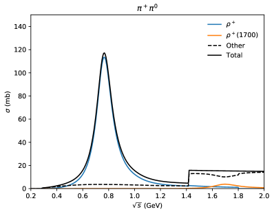
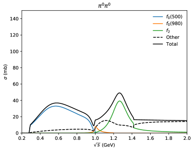
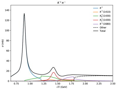
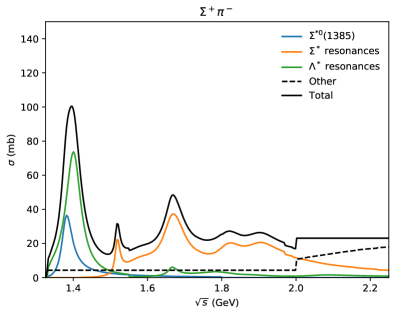
Figure 4: Resonant cross sections for some important cases, with partial cross sections for each resonance. For $p\pi^{0}$ and $\Sigma^{+}\pi^{-}$ there are many resonances, and we have divided them into groups for readability. The ”other” cross sections include elastic, diffractive and non-diffractive.

Explicit resonance formation has been implemented for $\pi\pi$, $\mathrm{K}\pi$, $\mathrm{N}\pi$, $\mathrm{N}\eta$, $\mathrm{N}\omega$, $\Sigma\pi$, $\Sigma\mathrm{K}$, $\Lambda\pi$, $\Lambda\mathrm{K}$, and $\Xi\pi$. This includes all isospin configurations of these particles where resonances exist (e.g. $\Sigma^{+}\pi^{-}$, but not $\Sigma^{-}\pi^{-}$). For the formation of a particular resonance $R$ the cross section is given by a nonrelativistic Breit–Wigner [46]

$$\sigma_{AB\to R}=\frac{\pi}{p_{\mathrm{CM}}^{2}}\frac{(2S_{R}+1)}{(2S_{A}+1)(2S_{B}+1)}\frac{\Gamma_{R\to AB}\Gamma_{R}}{(m_{R}-\sqrt{s})^{2}+\frac{1}{4}\Gamma_{R}^{2}}~{},$$ (23)

where $S$ is the spin of each particle, $p_{\mathrm{CM}}$ is the CM momentum of the incoming particles, $\Gamma_{R\to AB}$ is the mass-dependent partial width, and $\Gamma_{R}$ is the total mass-dependent width of $R$, found by summing the partial widths. The partial widths of a particle at mass $m$ are given by UrQMD as

$$\Gamma_{R\to AB}(m)=\Gamma_{R\to AB}(m_{0})\frac{m_{0}}{m}\frac{\left<p^{2l+1}(m)\right>}{\left<p^{2l+1}(m_{0})\right>}\frac{1.2}{1.0+0.2\frac{\left<p^{2l}(m)\right>}{\left<p^{2l}(m_{0})\right>}}~{},$$ (24)

where $m_{0}$ is the nominal mass of the particle and $\Gamma_{R\to AB}(m_{0})$ is the nominal width, both known from experiment, and $l$ is the angular momentum of the outgoing two-body system. The final factor ensures that widths do not blow up at large masses. The phase space factors are given by

$$\left<p^{2l+1}(m)\right>=\iint p_{\mathrm{CM}}^{2l+1}(m,m_{A},m_{B})\,A(m_{A})\,A(m_{B})\,\mathrm{d}m_{A}\,\mathrm{d}m_{B}~{},$$ (25)

where

$$p_{\mathrm{CM}}(m,m_{A},m_{B})=\frac{\sqrt{(m^{2}-(m_{A}+m_{B})^{2})(m^{2}-(m_{A}-m_{B})^{2})}}{2m}$$ (26)

and $A(m)$ are the mass distribution functions, given by a Breit–Wigner,

$$A(m)=\frac{1}{2\pi}\frac{\Gamma(m)}{(m^{2}-m_{0}^{2})^{2}+\frac{1}{4}\Gamma^{2}(m)},$$ (27)

which reduces to $A(m)=\delta(m-m_{0})$ for particles with zero width. Note that although the mass distribution depends on mass-dependent widths, which again depend on the mass distribution of other particles, there is no circular dependency since particle widths can only depend on the widths of lighter particles.

Figure 4 shows the resonant cross sections for some important cases. For the $\pi\pi$ cases there is a small elastic cross section below 1.42 GeV, corresponding to a d-wave contribution. For $\mathrm{K}^{+}\pi^{-}$ there is no direct elastic cross section at low energies, but a significant fraction of the resonances formed will decay back to the initial state particles, cf. Figure 3. We also observe a discontinuous behaviour at some points. One reason for this is that resonance particles are assigned a restricted mass range outside which they cannot be formed, which is particularly noticeable for example for $\mathrm{p}\pi^{0}\to\Delta^{+}$ at 2.0 GeV. Another reason for a non-smooth behaviour is the fact that the total cross section is parameterized using the more sophisticated machinery of [47, 48, 49] and the resonance cross sections are scaled to sum to this value. This is especially noticeable for $\pi^{+}\pi^{-}\to\rho^{0}$, where the total cross section is significantly larger than the sum of resonance cross sections in the range around 1.0-1.2 GeV, and is why the cross section for $\pi^{+}\pi^{-}\to\rho^{0}$ has a second peak in that region instead of looking like a regular Breit-Wigner. Both these kinds of discontinuities are visible in the $\mathrm{K}^{+}\pi^{-}$ cross sections, at the $K^{*}$ cutoff at 1.2 GeV.

One exceptional case is the formation of $f_{0}(500)$ resonances in $\pi^{+}\pi^{-}$ or $\pi^{0}\pi^{0}$ interactions. The nature of the $f_{0}(500)$ meson is not fully understood and it has certain exotic properties, notably its width is about the same as its mass. For this reason, eq. (23) does not describe its formation well. We find the relevant cross sections by interpolating values calculated based on the work by Peláez et al. [47, 48]. After the $f_{0}(500)$ has been produced, it is treated as any other meson, including in its decay.

The formula for mass-dependent partial widths works only for two-body decays. These are the dominant ones for most resonances we consider, but some hadrons have three- or four-body decays, for instance $\rho^{0}\to\pi^{+}\pi^{-}\pi^{+}\pi^{-}$. For such particles, we calculate the mass-dependent partial widths for the two-body channels according to eq. (24), but assume that the multibody channels have a constant width for the purposes of calculating the total width needed in eq. (23).

In the space–time description, the resonance is created at the average location of the two incoming hadrons at the interaction time in the collision CM frame. The resonance is then treated as any unstable particle with a mean lifetime that is assumed to be $\tau=1/\Gamma(m_{0})$, even if the resonance is off-shell. If all decay channels of the resonance are two-body decays, then eq. (24) is used to calculate the branching ratios. In this case, the masses of the outgoing particles are picked according to

$$\mathrm{d}\Gamma_{R\to AB}\sim p_{\mathrm{CM}}^{2l+1}(m,m_{A},m_{B})\,A(m_{A})\,A(m_{B})\,\mathrm{d}m_{A}\,\mathrm{d}m_{B}~{}.$$ (28)

If there is one or more multibody decay channels, the particle is instead decayed using the existing Pythia machinery.

3.4 Annihilation

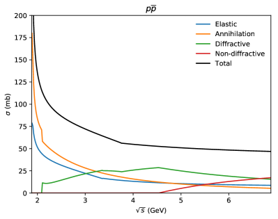
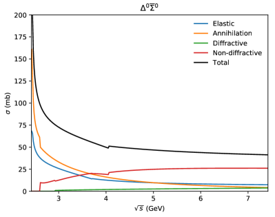
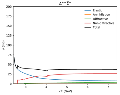
Figure 5: Partial cross sections for $\mathrm{p}\overline{\mathrm{p}}$, $\Delta^{0}\overline{\Sigma}^{0}$ and $\Delta^{++}\overline{\Sigma}^{+}$. We see that $\Delta^{0}\overline{\Sigma}^{0}$ is simply a rescaling of the $\mathrm{p}\overline{\mathrm{p}}$ case, except it gets different diffractive and non-diffractive contributions because $\mathrm{p}\overline{\mathrm{p}}$ implements explicit resonances. For $\Delta^{++}\overline{\Sigma}^{+}$ annihilation is not possible, so the annihilation cross section is subtracted from the total, significantly changing its shape.

In $\mathrm{B}\overline{\mathrm{B}}$ collisions the baryon number can be annihilated, so that only mesons remain in the final state. For $\mathrm{p}\overline{\mathrm{p}}$, below 2.1 GeV, annihilation counts for all inelastic processes, so below this threshold,

$$\sigma_{\mathrm{ann}}=\sigma_{\mathrm{tot}}-\sigma_{\mathrm{el}}.$$ (29)

Above the threshold, it is given by a parameterization by Koch and Dover [57],

$$\sigma_{\text{ann}}=120\frac{s_{0}}{s}\left(\frac{A^{2}s_{0}}{(s-s_{0})^{2}+A^{2}s_{0}}+0.6\right)~{},$$ (30)

where $s_{0}=4m_{p}^{2}$ and $A=0.05$ GeV. For other $\mathrm{B}\overline{\mathrm{B}}$, this is rescaled in the same way as for the total cross section. Note that the cross section is taken to be the same regardless of whether the baryons have one, two or three quarks in common, but if there are none then currently no annihilation is assumed, even though in principle it would be possible to decompose a $\mathrm{B}\overline{\mathrm{B}}$ system with no $\mathrm{q}\overline{\mathrm{q}}$ pairs in common into three separate $\mathrm{q}\overline{\mathrm{q}}$ strings. Figure 5 shows the cross sections for $\mathrm{p}\overline{\mathrm{p}}$, $\Delta^{0}\overline{\Sigma}^{0}$ and $\Delta^{++}\overline{\Sigma}^{+}$.

When an annihilation process occurs, one or two quark-antiquark pairs are annihilated. If two or more pairs are available, the probability for a second annihilation is given by a free parameter, by default 0.2, to represent a small but existing rate. No complete annihilation of all three pairs is performed, since the rate presumably is small and since it then would be necessary to recreate a new pair, making little net difference. The pair(s) to be annihilated is (are) chosen uniformly among all possible combinations. If only one quark pair remains, a single string is stretched between the $\mathrm{q}$ and $\overline{\mathrm{q}}$, along the original collision axis. If two pairs remain, a random pairing is done to form two separate strings. The procedure for sharing momentum is similar to the one described below in Section 3.6. The possibility of having a single string stretched between a diquark–antidiquark pair is omitted, since then a new baryon–antibaryon pair would be produced.

3.5 Diffractive processes

Diffractive cross sections in the continuous regime are calculated using SaS ansatz [56, 58]. The basic version of SaS is designed to deal only with processes involving $\mathrm{p}$, $\overline{\mathrm{p}}$, $\pi$, $\rho$, $\omega$ and $\phi$ (as needed for $\mathrm{p}\mathrm{p}/\gamma\mathrm{p}/\gamma\gamma$ collisions), and only for collision energies above 10 GeV. It is here extended to all baryons by applying an AQM rescaling factor to the corresponding $\mathrm{p}$ cross sections. For mesons a similar rescaling to $\pi$ ($=\rho$) cross sections is performed, except that here $\phi$ is retained as the template for $\mathrm{s}\overline{\mathrm{s}}$ interactions. The $\eta$ and $\eta^{\prime}$ cross sections thus are the appropriate mixes of $\pi$ and $\phi$ ones.

The differential cross section for single diffraction $AB\to XB$ is taken to be of the form

$$\mathrm{d}\sigma_{XB}\propto\frac{\mathrm{d}M_{X}^{2}}{M_{X}^{2}}\,\left(1-\frac{M_{X}^{2}}{s}\right)\,\exp(B_{XB}\,t)\,\mathrm{d}t~{},$$ (31)

where

$$B_{XB}(s)=2b_{B}+2\alpha^{\prime}\ln\left(\frac{s}{M_{X}^{2}}\right)~{},$$ (32)

with $b_{B}$ and $\alpha^{\prime}$ as for elastic scattering. The constant of proportionality involves hadron–pomeron and triple-pomeron couplings, specified for the few template processes and then multiplied by AQM factors. The diffractive mass spectrum is taken to begin at $M_{X,\mathrm{min}}=m_{A}+2m_{\pi}=m_{A}+0.28$ GeV and extend to the kinematical limit $M_{X,\mathrm{max}}=E_{\mathrm{CM}}-m_{B}$, while $t$ can take values within the full allowed range [23]. Above $E_{\mathrm{CM,min}}=10$ GeV the integrated cross section has been parameterized. Below this scale, our studies show that a shape like

$$\sigma_{XB}(E_{\mathrm{CM}})=\sigma_{XB}(E_{\mathrm{CM,min}})\,\left(\frac{E_{\mathrm{CM}}-M_{X,\mathrm{min}}-m_{B}}{E_{\mathrm{CM,min}}-M_{X,\mathrm{min}}-m_{B}}\right)^{0.6}$$ (33)

provides a good representation of the behaviour down to the kinematic threshold. Note that $m_{A}$ and $m_{B}$ are the actual masses of the colliding hadrons, not those of the corresponding template process.

Single diffraction $AB\to AX$ is obtained by trivial analogy with $AB\to XB$. For double diffraction $AB\to X_{1}X_{2}$ the cross section reads

$$\mathrm{d}\sigma_{XX}\propto\frac{\mathrm{d}M_{1}^{2}}{M_{1}^{2}}\,\frac{\mathrm{d}M_{2}^{2}}{M_{2}^{2}}\,\left(1-\frac{(M_{1}+M_{2})^{2}}{s}\right)\,\left(\frac{s\,m_{\mathrm{p}}^{2}}{s\,m_{\mathrm{p}}^{2}+M_{1}^{2}\,M_{2}^{2}}\right)\,\exp(B_{XX}\,t)\,\mathrm{d}t~{},$$ (34)

where

$$B_{XX}(s)=2\alpha^{\prime}\ln\left(e^{4}+\frac{s\,s_{0}}{M_{1}^{2}\,M_{2}^{2}}\right)~{},$$ (35)

again with $s_{0}=1/\alpha^{\prime}$. For the behaviour below 10 GeV, our studies suggest that

$$\sigma_{XX}(E_{\mathrm{CM}})=\sigma_{XX}(E_{\mathrm{CM,min}})\,\left(\frac{E_{\mathrm{CM}}-M_{X_{1},\mathrm{min}}-M_{X_{2},\mathrm{min}}}{E_{\mathrm{CM,min}}-M_{X_{1},\mathrm{min}}-M_{X_{2},\mathrm{min}}}\right)^{1.5}$$ (36)

is a suitable form.

So far we only considered the continuum production, which dominates for large diffractive masses. For small masses, diffractive cross sections can also include the formation of explicit resonances, and the contribution from these should be added to the continuum contribution. In our framework, this can occur as $\mathrm{N}\mathrm{N}\to\mathrm{N}\mathrm{N}^{*}$ or $\mathrm{N}\mathrm{N}\to\mathrm{N}\Delta^{*}$ (single diffractive), or $\mathrm{N}\mathrm{N}\to\Delta\mathrm{N}^{*}$ or $\mathrm{N}\mathrm{N}\to\Delta\Delta^{*}$ (double diffractive), and similarly when one baryon is replaced by its antibaryon. Higher excitations are implicitly part of the continuum diffractive treatment and not considered here. The cross section for $AB\to CD$ is given by Ref. [28]

$$\sigma_{AB\to CD}=(2S_{C}+1)\,(2S_{D}+1)\,\frac{1}{s}\frac{\left<p_{CD}\right>}{\left<p_{AB}\right>}\,|\mathcal{M}|^{2}~{},$$ (37)

where $S$ is the spin of each particle, $\mathcal{M}$ is the matrix element, and $\left<p_{ij}\right>$ are phase space factors given by eq. (25) (assuming $l=0$). In practice, this expression will sometimes lead to the sum of partial cross sections being larger than the total one. In those situations, we rescale the excitation cross sections (leaving other partial cross sections unchanged) so that the sum of partial cross sections is equal to the total.

For the matrix elements, we use the same as UrQMD [28]. For $\mathrm{N}\mathrm{N}\to N\Delta$ it is given by

$$|\mathcal{M}|^{2}=A\,\frac{m_{\Delta}^{2}\Gamma_{\Delta}^{2}}{(s-m_{\Delta}^{2})^{2}+m_{\Delta}^{2}\Gamma_{\Delta}^{2}}~{},$$ (38)

where $m_{\Delta}=1.232$ GeV and $\Gamma_{\Delta}=0.115$ GeV are the nominal mass and width of $\Delta$, and the coefficient is $A=40000$. For $\mathrm{N}\mathrm{N}\to\Delta\Delta$, the matrix element is a constant $|\mathcal{M}|^{2}=2.8$. Finally, for the remaining classes, the matrix element takes the form

$$|\mathcal{M}|^{2}=\frac{A}{(m_{C}-m_{D})^{2}(m_{C}+m_{D})^{2}}~{},$$ (39)

where $m_{C}$ and $m_{D}$ are the nominal masses for the outgoing particles (which will never be the same for these classes, so the matrix element cannot diverge), and the coefficient $A$ is $A=6.3$ for $\mathrm{N}\mathrm{N}\to\mathrm{N}\mathrm{N}^{*}$, $A=12$ for $\mathrm{N}\mathrm{N}\to N\Delta^{*}$, and $A=3.5$ for $\mathrm{N}\mathrm{N}\to\Delta N^{*}$ and $\mathrm{N}\mathrm{N}\to\Delta\Delta^{*}$.

In eq. (37), the only dependence on outgoing masses comes from the phase space term. Thus, the masses of the outgoing particles are distributed according to

$$\frac{\mathrm{d}\sigma_{AB\to CD}}{\mathrm{d}m_{C}\mathrm{d}m_{D}}\sim p_{\mathrm{CM}}(E_{\mathrm{CM}},m_{C},m_{D})\,A(m_{C})\,A(m_{D})~{},$$ (40)

from eq. (25). The $t$ behaviour is assumed to be given by an exponential slope with the same $B_{XB}/B_{XX}$ as in the continuum single/double diffraction for the given diffractive masses.

Calculating the integrals in eq. (25) during event generation would be debilitatingly slow. Therefore, we tabulate the cross sections for each process up to 8 GeV and use interpolation to get the total and partial excitation cross sections. For energies above this threshold, the expansion

$$p_{\mathrm{CM}}(E_{\mathrm{CM}},m_{C},m_{D})=\frac{1}{2}E_{\mathrm{CM}}\left(1-\frac{m_{C}^{2}+m_{D}^{2}}{E_{\mathrm{CM}}^{2}}+\mathcal{O}(E_{\mathrm{CM}}^{-3})\right)$$ (41)

shows that $p_{\mathrm{CM}}$ is approximately constant with respect to $m_{C}$ and $m_{D}$ when $E_{\mathrm{CM}}\gg m$. At the same time, the mass distributions $A(m)$ vanish at large $m$. Thus, in this limit, the phase factor can be approximated as

$$\left<p_{CD}\right>\approx p_{\mathrm{CM}}(E_{\mathrm{CM}},m_{C,0},m_{D,0})\int\mathrm{d}m_{C}\,A(m_{C})\int\mathrm{d}m_{D}\,A(m_{D}),$$ (42)

By integrating $A$ ahead of time, the cross sections can be calculated efficiently during run-time also above the tabulated region.

For other incoming hadron combinations, we fall back on the simpler smooth low-mass enhancement implemented in SaS to compensate for the lack of explicit resonances. For $AB\to XB$ the differential cross section in eq. (31) is multiplied by a factor

$$c_{\mathrm{res}}\,\frac{(m_{A}+M_{\mathrm{res},0})^{2}}{(m_{A}+M_{\mathrm{res},0})^{2}+M_{X}^{2}}~{}.$$ (43)

Here $c_{\mathrm{res}}=2$ and $M_{\mathrm{res},0}=2~{}\mathrm{GeV}-m_{\mathrm{p}}$ have been chosen to provide a decent description of the low-mass enhancement in $\mathrm{p}\mathrm{p}$ collisions at medium-high energies. For energies below 10 GeV this part of the cross section can be described in the same spirit as the continuum part in eq. (33), but the power is changed from 0.6 to 0.3. Double diffraction can be handled in the same spirit. Three terms contribute, where either side $A$, side $B$ or both are enhanced by a factor like eq. (43). In eq. (36) the power is changed from 1.5 to 1.25 for the first two and to 1.0 for the last one.

The kinematics of events is provided by the mass and $t$ selections outlined above. The decays of the explicit low-mass resonances are assumed to be isotropic. In the other cases a diffractive system is handled as a string stretched between two parts of the incoming hadron. A baryon is split into a diquark plus a quark at random, where the former/latter is moving in the forwards/backwards direction in the rest frame of the hadron. Here forwards is the direction the hadron will be moving out along, once boosted to the collision CM frame. A meson is correspondingly split into a quark plus an antiquark, but here the choice of which is moving forwards is taken to be random. The two string ends are given relative $p_{\perp}$ kicks of nonperturbative size, however, such that the string alignment along the collision axis is smeared.

Figure 6a shows all partial cross sections for $\mathrm{p}\mathrm{p}$ collisions. We see that the single diffractive cross section is very small compared to other cross sections, and the double diffractive one almost vanishes. The excitation cross section is here shown separately from the cross sections describing diffraction in the continuous region. Note that below around 4.5 GeV, the excitation cross section is set equal to the difference $\sigma_{\mathrm{tot}}-\sigma_{\mathrm{el}}$ instead of following the form given by eq. (37). The full shape of the excitation cross sections are shown in Figure 6b.

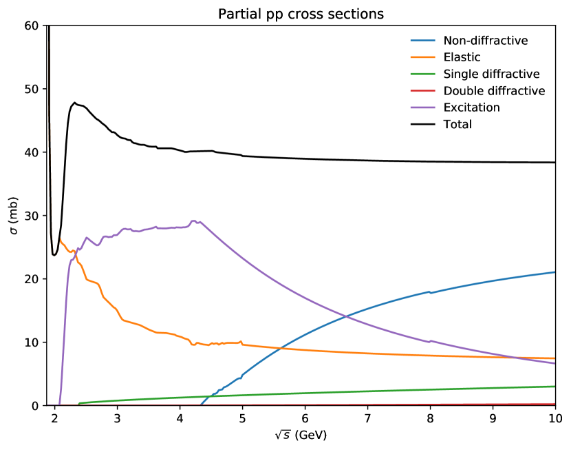
(a)

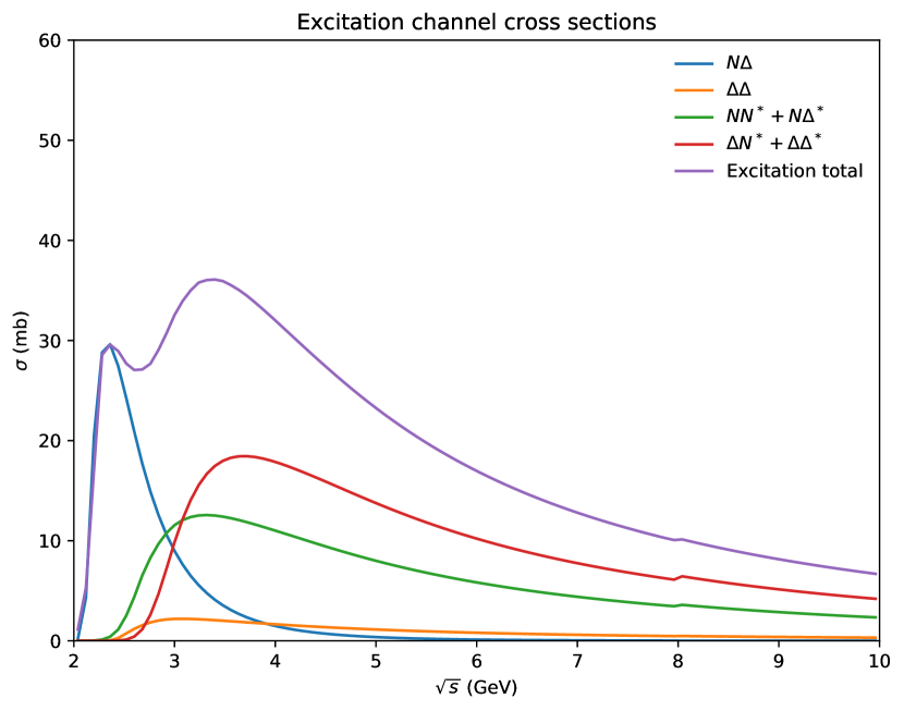
(b)

Figure 6: (a) All partial cross sections for $\mathrm{p}\mathrm{p}$ interactions. (b) Excitation cross sections, according to eq. (37). Note the small jump at 8 GeV, at the boundary between the tabulated and parameterized regions.

3.6 Nondiffractive processes

Nondiffractive cross sections are found by subtracting all other partial cross sections from the total cross section,

$$\sigma_{\mathrm{nondiff}}=\sigma_{\mathrm{tot}}-\sigma_{\mathrm{el}}-\sigma_{\mathrm{diff}}-\sigma_{\mathrm{res}}-\sigma_{\mathrm{ann}}.$$ (44)

At large energies the nondiffractive processes dominate the total cross section, but at low energies they can have a small or even vanishing cross section. Since it is defined as the difference between the total and the other partial cross sections, it can sometimes have a fluctuating energy dependence with no clear physics explanation.

A nondiffractive event is associated with the exchange of a gluon between the two incoming hadrons, where the gluon carries negligible momentum but leads to a rearranged colour topology. To this end, each initial hadron is separated into a colour (a quark or an antidiquark) part and an anticolour (an antiquark or a diquark) part. For a baryon the selection of the diquark part is done according to the $SU(6)$ decomposition (in three flavours times two spins), while the meson subdivision is trivial. After the colour-octet gluon exchange, the colour end of one hadron forms a colour singlet with the anticolour end of the other hadron, and vice versa. (Cases with more complicated colour-charge topologies are suppressed and are neglected here.) This leads to two strings being stretched out between the two octet-state “hadrons”.

Consider the collision in its rest frame, with hadron $A$ ($B$) moving in the $+z$ ($-z$) direction. In that frame, the colour and anticolour objects of each hadron are assumed to have an opposite and compensating $p_{\perp}$. This is chosen according to a Gaussian with the same width as used to describe the $p_{\perp}$ smearing in string breakup vertices. In the breakup context a width of $\langle p_{\perp}^{2}\rangle\approx(0.35~{}\mathrm{GeV})^{2}$ is motivated by a tunnelling mechanism, but a number of that magnitude for the parton motion inside a hadron could equally well be viewed as a consequence of confinement in the transverse directions by way of the Heisenberg uncertainty relations.

Including (di)quark masses, the transverse masses $m_{\perp A1}$ and $m_{\perp A2}$ of the two $A$ hadron constituents are defined. Next a $z_{A}$ value is picked that splits the $A$ lightcone momentum $p_{A}^{+}=E_{A}+p_{zA}$ between the two, $p_{A1}^{+}=z_{A}p_{A}^{+}$ and $p_{A2}^{+}=(1-z_{A})p_{A}^{+}$ [39]. For a meson $z=x_{1}/(x_{1}+x_{2})$, where the $x_{i}$ are picked at random according to $(1-x_{i})^{0.8}/\sqrt{x_{i}}$. For a baryon first each of the three quarks are assigned an $x_{i}$ according to $(1-x_{i})^{2.75}/\sqrt{x_{i}}$. If $z_{A}$ is associated with the diquark, made out of the first two quarks, then $z_{A}=2(x_{1}+x_{2})/(2(x_{1}+x_{2})+x_{3})$. Note that here the diquark tend to take most of the momentum, not only because it consists of two quarks, but also by an empirical enhancement factor of 2. The $p_{Ai}^{-}$ can now be obtained from $p^{+}p^{-}=m_{\perp}^{2}$, and combined to give an effective mass $m_{A}^{*}$ that the $A$ beam remnant is associated with: $m_{A}^{*2}=m_{\perp A1}^{2}/z+m_{\perp A2}^{2}/(1-z)$. The same procedure can be repeated for the $B$ hadron, but with $p^{+}\leftrightarrow p^{-}$. Together, the criterion $m_{A}^{*}+m_{B}^{*}<E_{\mathrm{CM}}$ must be fulfilled, or the whole selection procedure has to be restarted. (Technically, some impossible values can be rejected already at earlier stages.) Once an acceptable pair $(m_{A}^{*},m_{B}^{*})$ has been found, it is straightforward first to construct the kinematics of $A^{*}$ and $B^{*}$ in the collision rest frame, and thereafter the kinematics of their two constituents.

Since the procedure has to work at very small energies, some additional aspects should be mentioned. At energies very near the threshold, the phase space for particle production is limited. If the lightest hadrons that can be formed out of each of the two new singlets together leave less than a pion mass margin up to the collision CM energy, then a simple two-body production of those two lightest hadrons is (most likely) the only option and is thus performed. There is then a risk to end up with an unintentional elastic-style scattering. For excesses up to two pion masses, instead an isotropic three-body decay is attempted, where one of the strings breaks up by the production of an intermediate $\mathrm{u}\overline{\mathrm{u}}$ or $\mathrm{d}\overline{\mathrm{d}}$ pair. If that does not work, then two hadrons are picked as in the two-body case and a $\pi^{0}$ is added as third particle.

One reason why $m_{A}^{*}+m_{B}^{*}<E_{\mathrm{CM}}$ might fail is if the constituent transverse masses are too big. Thus, after a number of failed attempts, their values are gradually scaled down to increase the likelihood of success. This, on the other hand, increases the risk of obtaining two strings with low invariant masses. A further check is therefore made that each string has a mass above that of the lightest hadron with the given flavour content, and additionally that the mass excess is at least a pion mass for one of the two strings.

The two strings can now be hadronized, but often one or both have small masses. To this end the ministring framework, used when at most two hadrons can be formed from a string, has been extended to try harder. Several different approaches are used in succession, until one of them works. The order is as follows.
(1) Several attempts are made to produce two hadrons from the string by a traditional string break in the middle.
(2) If not, a hadron is formed consistent with the endpoint flavour content. Four-momentum is shuffled between it and one of the partons of the other string, so as to put the hadron on mass shell while conserving the overall four-momentum. Since the string with lowest mass excess is considered first, the two partons of the other string should normally be available.
(3) If no allowed shuffling is found, then a renewed attempt is made to produce two hadrons by a string break, but this time the two lightest hadrons of the given flavour content are chosen.
(4) If that does not work, one lightest hadron is formed from the endpoint flavours and the other is set to be a $\pi^{0}$.
(5) It still no success, then go back to forming one hadron, but the lightest possible, and again shuffle momentum to a parton.
(6) Finally, the problem may occur also for the string with higher mass excess, i.e. after the first string was hadronized, and possibly took some four-momentum in the process. Then a collapse to one hadron (at random or eventually the lightest) with the recoil taken by another hadron is attempted.

3.7 The transition to high-energy processes

We have now described a framework for low energy hadron-hadron interactions. Our motivation for doing this has been to apply it to rescattering, but in principle, having this framework means that it is now possible to generate events in Pythia at these low energies. Despite all the technical details, the structure of the resulting events is quite simple. At most two objects (either hadrons or strings) are created in the first step of the process. The strings are stretched out almost perfectly along the collision axis and fragment into hadrons with only small nonperturbative $p_{\perp}$ kicks.

This is in contrast to the high-energy framework used to simulate the primary LHC $\mathrm{p}\mathrm{p}$ collision, e.g. in inelastic nondiffractive processes. Here the multiparton interactions machinery very much is based on perturbation theory, where each interaction requires the use both of hard matrix elements and parton distribution functions (PDFs), giving scattered partons over a wide range of $p_{\perp}$ scales, even if the lower scales dominate. Many string pieces are stretched criss-cross in the event, and fragment into the high-multiplicity initial state that the rescattering framework will be applied to. If one uses this perturbative framework at lower and lower energies the average number of MPIs will decrease, as will their typical $p_{\perp}$ scale. Gradually the idea of applying a perturbative approach becomes less appealing. Technically the machinery can be applied down to 10 GeV CM energy, but is then highly questionable. Furthermore, many of the cross sections described here do not scale correctly at higher energies. For a high-energy $\mathrm{p}\mathrm{p}/\mathrm{p}\overline{\mathrm{p}}$ primary collision four different models are available [59]. Only one of them explicitly covers some more collision types, but extensions by AQM rescaling could be possible.

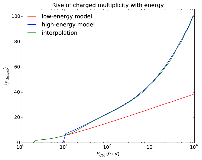
(a)

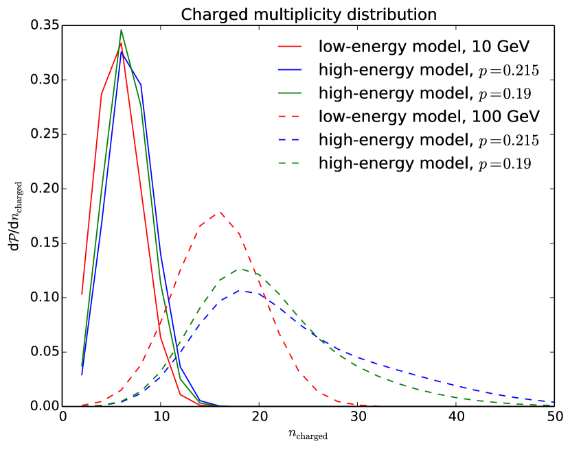
(b)

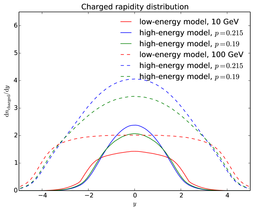
(c)

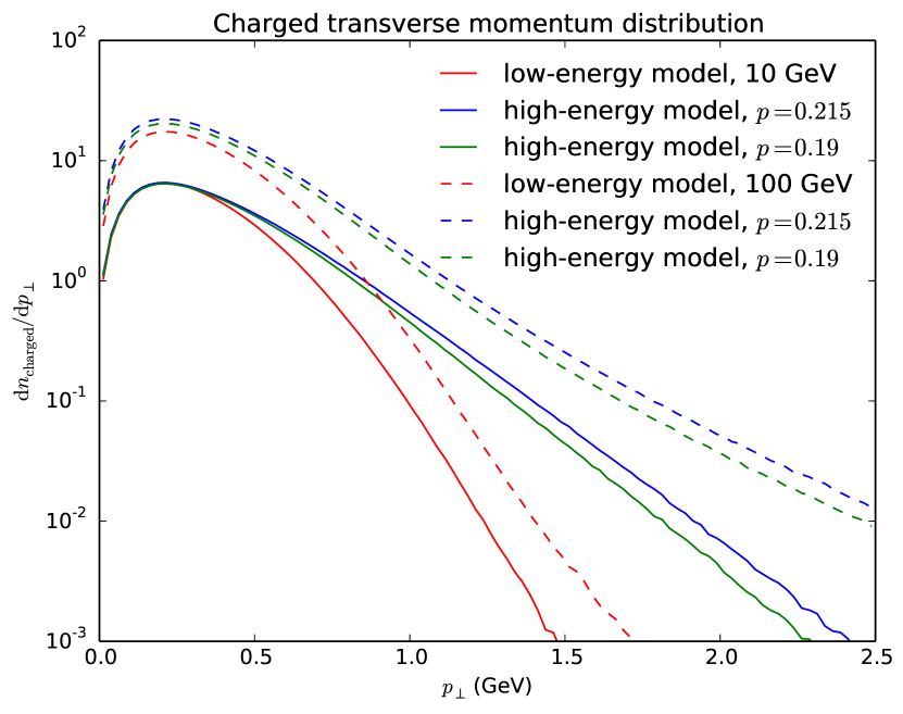
(d)

Figure 7: (a) Energy dependence of the average charged multiplicity in nondiffractive $\mathrm{p}\mathrm{p}$ collisions. (b,c,d) Comparison of charged multiplicity, rapidity and transverse momentum distributions for 10 and 100 GeV nondiffractive $\mathrm{p}\mathrm{p}$ collisions.

Therefore it is tempting to interpolate between the two descriptions. There is now such an option available. In it, the fraction of perturbatively handled events rises from the threshold energy $E_{\mathrm{thr}}=10$ GeV as

$$P_{\mathrm{pert}}=1-\exp\left(-\frac{E_{\mathrm{CM}}-E_{\mathrm{thr}}}{E_{\mathrm{wid}}}\right)~{},$$ (45)

where $E_{\mathrm{wid}}=10$ GeV is a measure of the size of the transition region. This is actually the same form as already used previously to transition between a nonperturbative and a perturbative description of diffraction, with the diffractive system mass replaced by $E_{\mathrm{CM}}$ [60, 59].

How this transition works in practice is illustrated in Figure 7a, for the energy dependence of the charged multiplicity in nondiffractive events. In this figure the difference between the low-energy and high-energy model multiplicities is not so large in the transition range 10 – 30 GeV, but the importance of the perturbative components obviously increases with energy. Zooming in on the behaviour at the 10 GeV threshold and at an energy above it, at 100 GeV, Figure 7b,c,d show some differential distributions. At 10 GeV the limited phase space does not allow for high multiplicities, while a longer perturbatively-induced tail is apparent at 100 GeV. Nevertheless, the MPI activity is reflected in a shift towards central rapidities and the presence of a high-$p_{\perp}$ tail already at 10 GeV.

The perturbative model results have been obtained with the default Monash tune [61], which mainly is based on comparisons with LEP, Tevatron and LHC data. One should therefore be aware that the extrapolation to lower energies is not without its problems. As an example, the key parameter of the MPI framework is the $p_{\perp 0}$ one, that regularizes the divergence of the perturbative $2\to 2$ cross sections in the limit $p_{\perp}\to 0$. It is assumed to have an energy dependence that scales like $p_{\perp 0}\propto E_{\mathrm{CM}}^{p}$ (but more complicated forms could be considered). The default values, with $p=0.215$, gives $p_{\perp 0}=0.56$ and 0.91 GeV, respectively, at 10 and 100 GeV. If $p$ is changed to 0.19, then instead $p_{\perp 0}=0.66$ and 1.02 GeV, respectively, at the low energies, assuming a fixed $p_{\perp 0}$ value at 7 TeV. The result of such a modest change is illustrated in Fig. 7b,c,d. Qualitatively the difference to the low-energy model remains, but quantitatively it is visibly reduced.

One may also note that the string drawing can be quite different in the two cases. In the nonperturbative model the $\mathrm{p}\mathrm{p}$ events always are represented by two strings, each stretched between a quark and a diquark. When MPIs are included, it becomes frequent that two quarks are kicked out of the same proton, more so at low energies where the high-$x$ valence-quark part of PDFs is probed. This leads to so-called junction topologies, where the baryon number can wander more freely in the event [62]. Technically, this makes the hadronization of low-energy events more messy, and may require repeated attempts to succeed.

In diffraction, the excited masses $M_{X}$ vary between events, also for a fixed CM energy. To handle perturbative activity inside the diffractive system then would seem to require a time-consuming re-initialization of the MPI framework for each new diffractive system. Instead, at the beginning of a run, an initialization is done for a set of logarithmically spaced diffractive masses, and numbers relevant for the future generation are saved in arrays. By interpolation, required numbers can then be found for any mass during the subsequent event generation. This approach has now been extended also to be available for nondiffractive processes, if so desired. This means that $\mathrm{p}\mathrm{p}$ collisions can be simulated essentially from the threshold to LHC energies and beyond without any need to re-initialize. The prize to pay is a somewhat longer initialization step at the beginning of a run, but still in the range of seconds rather than minutes. One current limitation is that it is numbers for the MPI generation that are stored, so it is not now possible to pick a specific hard process for handling in the same way.

Another limitation is that the perturbative framework requires access to PDFs for the colliding hadrons, which restricts us to $\mathrm{p}$, $\mathrm{n}$ and (with big uncertainties) $\pi$. Additionally PDFs are available for the photon and the pomeron, the latter used in diffraction, and in that sense they can be handled on equal footing with hadrons. A further restriction is that Pythia can only be set up for one combination of incoming beams at a time, so as to handle the perturbative processes. The simpler nonperturbative machinery used for rescatterings has no such restriction, of course.

4 Model tests

In this section, we will study the properties of the rescattering model. We start with studying how rescattering affects simple observables such as $p_{\perp}$ spectra, charged multiplicity, jet structure, and the potential for collective flow. We also look at how event properties change when rescattering is performed in a Lorentz boosted frame, in order to verify that the frame-dependence described in Section 2.3 does not significantly alter the final state.

Next, we look at the rates at which different particle types participate in rescattering and the rates at which the different types of processes occur. Finally, we consider the free parameters and model choices that have gone into the framework, and study the effect of changing those.

4.1 Basic effects of rescattering

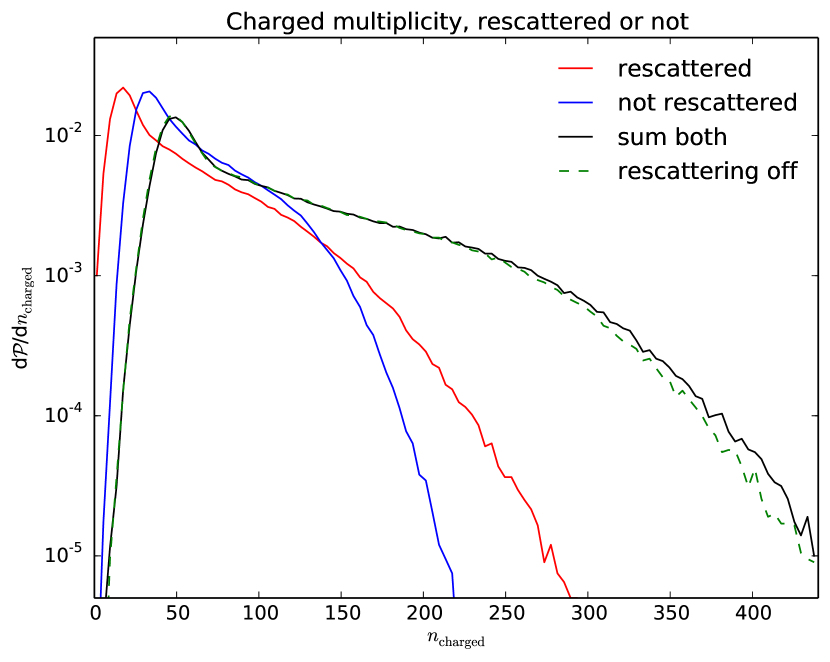
(a)

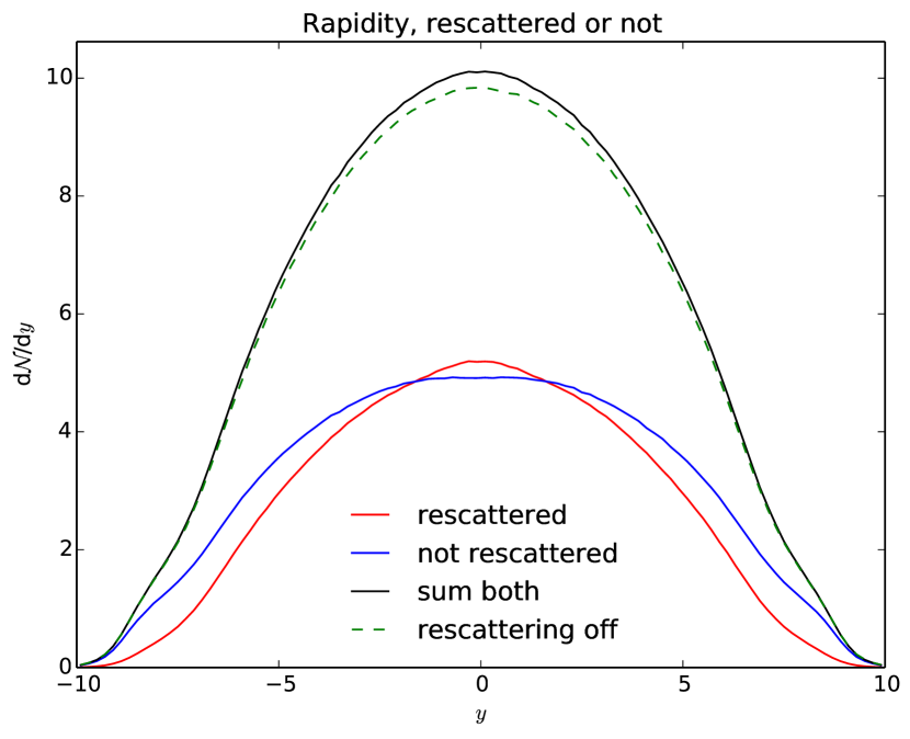
(b)

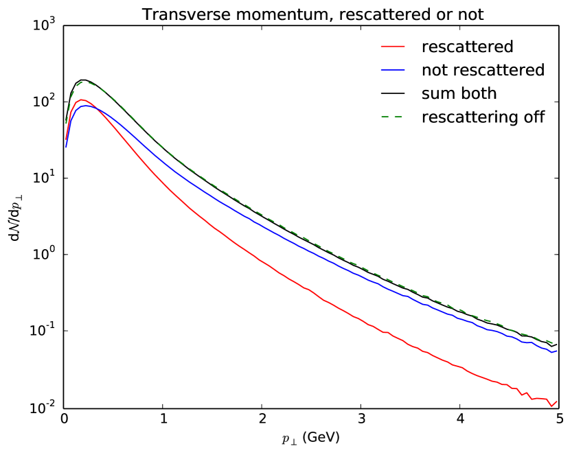
(c)

(d)

Figure 8: (a) Multiplicity, (b) rapidity, (c) transverse momentum, and (d) invariant production time spectra of charged final-state hadrons, subdivided into those that have been involved in rescatterings and those that have not, in 13 TeV nondiffractive $\mathrm{p}\mathrm{p}$ events. As reference a comparison is also made with events without rescatterings.

As the most basic check, Figure 8 shows how charged multiplicity, rapidity spectra, transverse momentum spectra, and invariant production times are affected by rescattering. We see that rescattering increases charged multiplicity, which is obviously expected when one considers the fact that we have implemented $2\to n$, $n\geq 3$ interactions, but not interactions involving multiple incoming particles. The rescatter-affected hadrons have a broader multiplicity distribution than those not involved: events that start out with a low number of primary hadrons have a smaller rescattering probability than average, and vice versa.

In the same vein, the rescattered fraction is larger for central rapidities, where there are more hadrons to begin with, and this is also where inelastic rescatterings give a multiplicity increase. An interesting observation is that higher-$p_{\perp}$ hadrons seldom participate in rescattering, Figure 8c. The natural explanation is that these hadrons typically are produced at larger transverse distances by (mini)jet fragmentation, where the particle density is reduced by having fewer overlapping MPI systems than at small $r_{\perp}$. Notable is also the slight net decrease at high $p_{\perp}$ by rescattering, (over)compensated by the increase at small $p_{\perp}$. Finally, and quite logically, rescattering kicks in with some delay in invariant time, since a sufficient amount of primary hadrons have to be produced first.

The point of introducing rescattering is to change some event properties, but not all changes are relevant rescattering signals, since some could easily be compensated by a retuning of many other parameters. In particular, the average (charged) event multiplicity is such a signal. Indeed, the fact that it is changed by rescattering means that a retune is necessary in order to restore it to the experimentally well-known value. The MPI framework, which is the main driving force in generating the multiplicity spectrum, is sufficiently uncertain to easily absorb the rescattering effects on the multiplicity. More specifically, when we study the effects of rescattering, the $p_{\perp 0}$ parameter of the MPI framework, MultipartonInteractions:pT0Ref, is adjusted to restore the average charged multiplicity in the $\eta<2.5$ range to the no-rescattering value. Its default value in Pythia is pT0Ref = 2.28 (GeV), and we have found that setting it to pT0Ref = 2.345 restores charged multiplicity to the correct value. We will use this value in all subsequent studies, unless otherwise noted. In the future, a more detailed retune would be desirable.

4.2 Jets

(a)

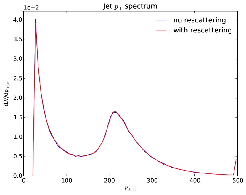
(b)

Figure 9: Production rates (a) and inclusive $p_{\perp}$ spectra (b) of jets in 13 TeV $\mathrm{p}\mathrm{p}$ collisions, as further described in the text. The uptick in the last bin of (b) is because all jets with $p_{\perp}>500$ GeV have been put there.

We have already argued that high-$p_{\perp}$ particles are less affected by rescattering than low-$p_{\perp}$ ones, and hence jets should remain essentially unchanged. This also turns out to be the case. As an example, QCD two-jet production with $p_{\perp}>200$ GeV hard collisions at 13 TeV was studied, and anti-$k_{\perp}$ jets found for a 0.7 radius and a 25 GeV lower cut-off [63]. We then find that the particle multiplicity inside a jet with rescattering on is about 2% higher than with rescattering off. This increase is almost uniformly spread from the center to the periphery of the jet. The $p_{\perp}$-weighted jet profile is almost identical, however. Studying the jet rate itself, there is a small net reduction in the number of jets when rescattering is allowed, Figure 9a. The difference is too small to be visible in the jet $p_{\perp}$ spectrum, Figure 9b. A closer inspection shows that the jet rate above 150 GeV, i.e. in the domain of the two hard jets, is unchanged within statistics. Below that scale, however, i.e. mainly additional jets from parton showering, there is a drop by about 2% in the rate. This is most likely related to a slight leakage of hadrons out of the jet cone, shifting jet energies ever so slightly downwards. Such tiny differences could easily be tuned away, so in the end we conclude that jet properties are not measurably affected.

4.3 Collective flow

One of the telltale signs of collective behaviour is an anisotropy in the azimuthal angle of outgoing particle momenta. Here we perform a preliminary study to see whether rescattering can produce azimuthal flow at all.

In order to obtain a systematic flow, two things are required: an initial spatial anisotropy and a mechanism for collective behaviour. In this toy study an anisotropy is obtained by selecting the primary $\mathrm{p}\mathrm{p}$ collisions to have their impact parameter aligned along the $x$ axis, and choosing MPI vertices according to a Gaussian distribution multiplied by a $\varphi$ modulation factor with $\epsilon=0.5$ (see Section 2.2). The resulting $x$-$y$ anisotropy of primary hadron production is illustrated in Figure 10a. This causes an elliptic flow, as shown in Figure 10b, where the $\varphi$ angle of final particle momenta is relative to the $x$ axis (which we know to be our event plane). By the symmetry of the initial anisotropy, the shape of the spectrum should depend only on the acute angle to the event plane, $0<\varphi<\pi/2$, and we reduce the spectrum to this range to obtain better statistics.

The flow is aligned in the $y$-direction, consistent with the higher density gradient in this direction. Results are binned according to the charged multiplicity, which is correlated with the impact parameter. A low multiplicity is associated with peripheral events, for which the spatial anisotropy may be strong, but collective behaviour is suppressed by the low density. A high multiplicity, on the other hand, indicates a central event with much rescattering, but a low impact parameter so a less strict azimuthal alignment. In our simple study these two effects largely cancel to give comparable asymmetries independently of the multiplicity.

Unfortunately, the aforementioned study has been made under the unrealistic advantage of a known event plane. In practice one would rather study e.g. two-particle azimuthal correlations. Furthermore, the initial anisotropy has been made implausibly large for illustratory purposes. When the simulation is repeated with more reasonable assumptions, we no longer observe any signs of flow. Therefore this brief study should be regarded as a proof of concept, and we hope to return to flow studies in the context of heavy-ion collisions, where a strong spatial anisotropy occurs naturally.

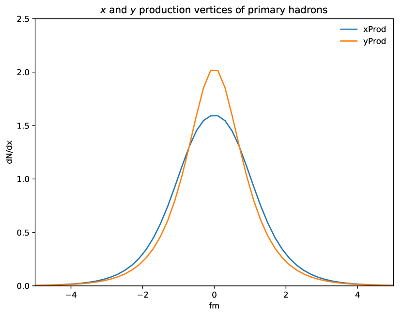
(a)

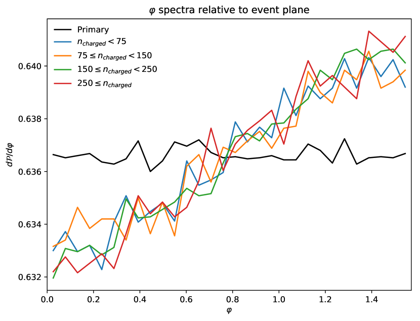
(b)

Figure 10: (a) $x$ and $y$ coordinates of primary hadrons, showing an initial anisotropy. (b) Azimuthal direction of momentum for outgoing hadrons, binned according to charged multiplicity. The angle is the acute angle to the event plane, $\varphi\in[0,\pi/2]$. The plot includes the spectrum for the primary hadrons, which illustrates that there is no flow before a collective behaviour has been induced by rescattering.

4.4 Lorentz frame dependence

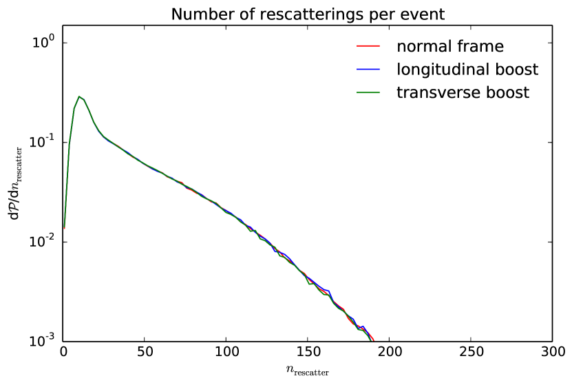
(a)

(b)

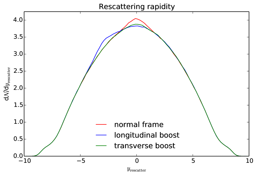
(c)

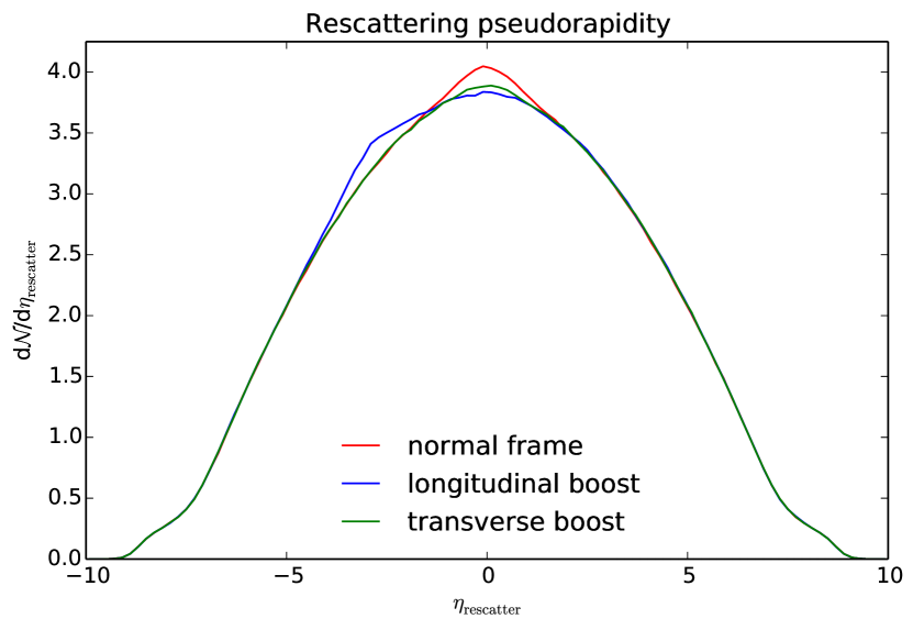
(d)

(e)

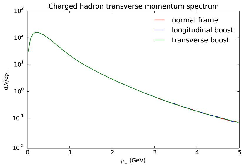
(f)

Figure 11: Effects of modified time ordering on 13 TeV pp nondiffractive collisions, where ordering is either in the normal rest frame, or in a frame boosted either longitudinally or transversely by three units of rapidity. (a) Number of rescatterings. (b) Invariant mass distribution of rescatterings. (c) Rapidity distribution of rescatterings. (d) Distribution in $\eta=(1/2)\,\ln((t+z)/(t-z))$ of rescatterings. (e) Rapidity distribution of final charged hadrons. (f) Transverse momentum spectrum of final charged hadrons.

The time ordering of rescatterings is not Lorentz invariant but, we do not expect this to be a major issue, since most potential rescatterings cannot influence each other. To confirm this more thoroughly, we boost the events by three units of rapidity either along or transverse to the collision axis, perform rescattering in this boosted frame, then boost back afterwards. Some results of performing this procedure, compared with the ones in the normal CM frame, are shown in Figure 11. One may first note that the number of rescatterings and their invariant mass distribution are essentially unchanged. The rapidity spectrum of rescatterings however is somewhat deformed by the forward boost, where rescatterings would begin at around $y=-3$. Such rescatterings thus in part preempt ones at larger times in that frame. The same applies for the space–time pseudorapidity, $\eta=(1/2)\,\ln((t+z)/(t-z))$. If instead the boost is transverse, the effects on the $y$ and $\eta$ spectra are even smaller. Here collisions on the $-x$ side of the event get an earlier start than those on the $+x$ one, giving a $\pm 2$% modulation in the azimuthal distributions of rescatterings (not shown). These effects average out in other distributions, however, so that the $p_{\perp}$ and $r_{\perp}=\sqrt{x^{2}+y^{2}}$ rescattering spectra are almost unchanged by transverse and longitudinal boost alike.

At the end of the day, the real test is whether observable properties are affected or not. Figure 11e,f show that the final-state charged-hadron rapidity and $p_{\perp}$ spectra are almost completely insensitive to the choice of rest frame. The same also applies for other distributions we have studied, such as the azimuthal dependence, or the separate $\pi/\mathrm{K}/\mathrm{p}$ spectra. The breach of Lorentz frame independence therefore is a negligible issue for our studies.

4.5 Rescatter rates

(a)

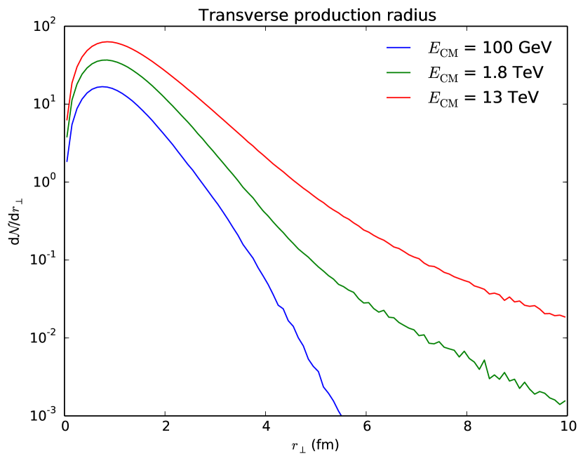
(b)

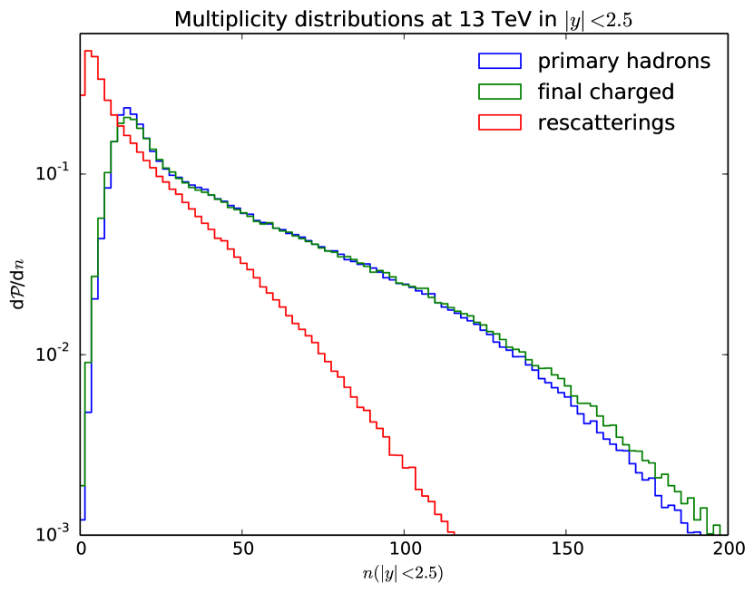
(c)

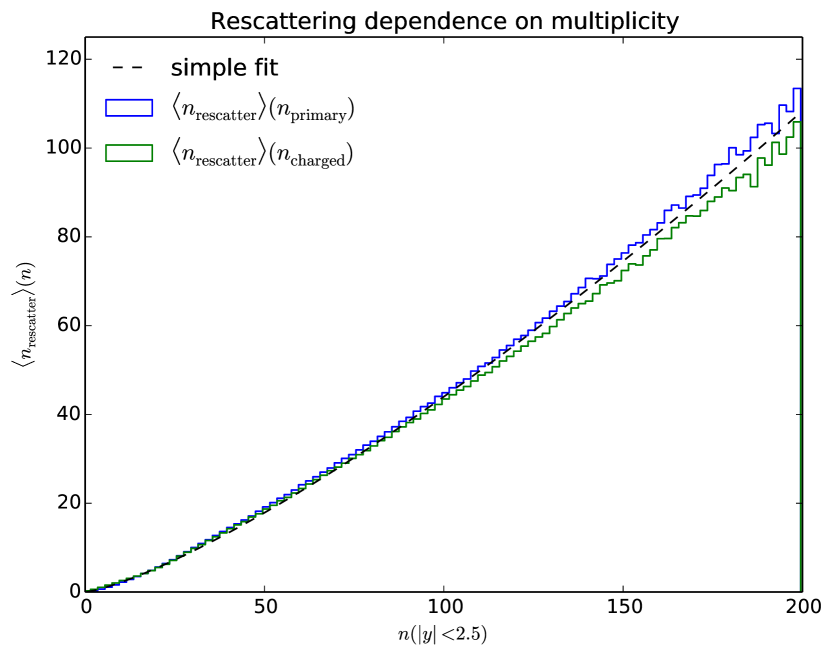
(d)

Figure 12: (a) Energy dependence of multiplicities in nondiffractive $\mathrm{p}\mathrm{p}$ collisions. (b) Primary hadron production in $r_{\perp}=\sqrt{x^{2}+y^{2}}$ at three energies. (c) Distribution in the numbers of primary hadrons, charged hadrons and rescatterings in the central $|y|<2.5$ region of 13 TeV nondiffractive $\mathrm{p}\mathrm{p}$ collisions. (d) Multiplicity dependence of the number of rescatterings in events as above.

In this section we study how common rescatterings are, both overall and subdivided by hadron species and by process types. The average number of rescatterings per (inelastic) nondiffractive $\mathrm{p}\mathrm{p}$ event is shown as a function of the collision energy in Figure 12a. It is compared to the primary hadron multiplicity, i.e. the hadrons produced directly from the fragmenting strings, and to the final charged multiplicity. Note that these latter two are almost equal; the multiplicity increase from the decays of primary hadrons is compensated by the decrease from the exclusion of neutral particles. This largely holds also on an event-by-event level, so we may use the observable charged multiplicity as a simple measure of number of primary hadrons that may rescatter. As an order-of-magnitude, the average number of rescatterings $\langle n_{\mathrm{rescatter}}\rangle$ is about half that of the primary multiplicity $\langle n_{\mathrm{primary}}\rangle$. While the number of potentially colliding pairs increases like $n_{\mathrm{primary}}^{2}$, the dashed line represents a fit according to a much slower $\langle n_{\mathrm{primary}}\rangle^{1.2}$. The reason is that the system size also increases with energy. Obviously so in the longitudinal direction, but also in the transverse one, by an increasing MPI perturbative activity spreading production vertices over a larger transverse area, Figure 12b.

Zooming in on the central rapidity region of 13 TeV nondiffractive events, the different kinds of multiplicity distributions are displayed in Figure 12c, and the rescattering rate as a function of the primary or charged multiplicity in Figure 12d. In the latter, a simple fit $\langle n_{\mathrm{rescatter}}\rangle\propto n_{\mathrm{primary}}^{1.3}$ has been inserted to guide the eye, showing a similar scaling as for the energy dependence. The power 1.3 also describes the dependence in the event as a whole, without the $|y|<2.5$ restriction.

incoming	rate	incoming	rate	incoming	rate
$\pi+\pi$	12.63	$\mathrm{K}+\mathrm{N}$	0.39	$\eta/\eta^{\prime}+N$	0.19
$\pi+\rho$	4.59	$\rho+\rho$	0.38	$\pi+\mathrm{B}$	0.18
$\pi+\mathrm{K}$	3.84	$\rho+\mathrm{N}$	0.36	$N+\Delta$	0.16
$\pi+\mathrm{N}$	3.44	$\rho+\omega/\phi$	0.34	$\pi+\Sigma^{*}$	0.15
$\pi+\omega/\phi$	2.08	$\rho+\eta/\eta^{\prime}$	0.30	$\rho+\Delta$	0.14
$\pi+\eta/\eta^{\prime}$	1.80	$\pi+f_{0}(500)$	0.29	$\eta/\eta^{\prime}+\omega/\phi$	0.14
$\pi+\mathrm{K}^{*}$	1.33	$\mathrm{K}+\omega/\phi$	0.27	$\pi+\mathrm{M}$	0.12
$\pi+\Delta$	1.10	$\mathrm{K}+\mathrm{K}$	0.26	$\mathrm{K}+\Delta$	0.11
$\rho+\mathrm{K}$	0.54	$\pi+\Lambda$	0.25	$\mathrm{K}^{*}+\mathrm{N}$	0.11
$\pi+\Sigma$	0.46	$\omega/\phi+\mathrm{N}$	0.24
$\mathrm{N}+\mathrm{N}$	0.46	$\mathrm{K}+\eta/\eta^{\prime}$	0.23
$\mathrm{K}+\mathrm{K}^{*}$	0.41	$\rho+\mathrm{K}^{*}$	0.20	other	1.87

Table 6: Number of collisions per 13 TeV nondiffractive $\mathrm{p}\mathrm{p}$ event, of different incoming particle combinations, where particles have been grouped so as to avoid too fragmented a view. $\mathrm{M}$ represents other meson species and $\mathrm{B}$ other baryon ones. All combinations with a rate below 0.1 have been summed into the “other” group.

Process type	rate
resonant	17.80
elastic	14.08
nondiffractive	6.92
annihilation	0.49
diffraction + excitation	0.05

Table 7: Number of collisions of different types per 13 TeV nondiffractive $\mathrm{p}\mathrm{p}$ event.

With well over a hundred different hadron species that can be produced, the number of different colliding hadron pairs are in the thousands, even if most of them are quite rare. To give some feel, Table 6 shows the most common groups of hadron pairs. Here $\pi$ represents all pions, $\mathrm{K}$ all Kaons ($\mathrm{K}^{\pm}$, $\mathrm{K}^{0}$, $\overline{\mathrm{K}}^{0}$, $\mathrm{K}_{\mathrm{S,L}}^{0}$), $\mathrm{N}$ all nucleons ($\mathrm{p}$, $\mathrm{n}$, $\overline{\mathrm{p}}$, $\overline{\mathrm{n}}$), and so on. As can be seen, $\pi\pi$ rescatterings dominate by far, constituting about a third of all rescatterings, while $\pi$ with anything else constitutes another third. This highlights the importance of accurate cross sections for processes involving pions.

Collisions are also characterized by which type of process occurs, Table 7. The resonant, elastic and nondiffractive types dominate by far. Baryon–antibaryon annihilation is small but not negligible for the baryon subclass of particles. Diffraction and excitation require more phase space to occur, and therefore become suppressed.

(a)

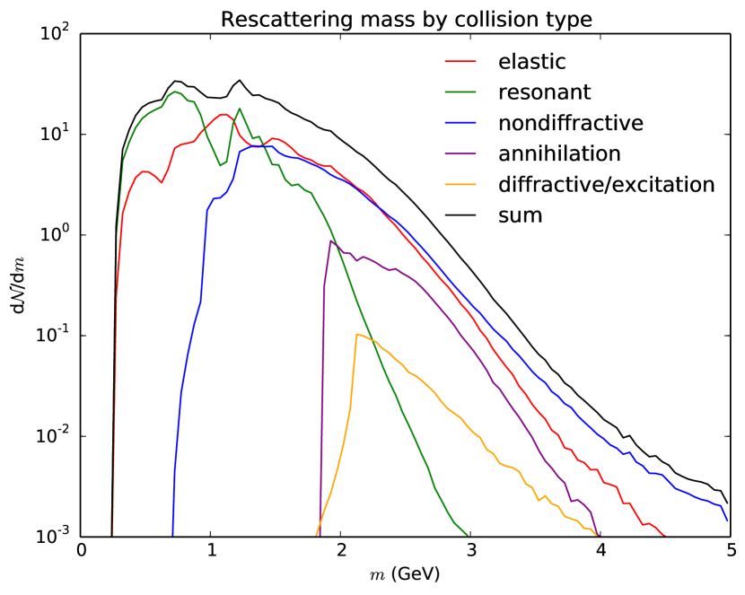
(b)

Figure 13: Invariant mass distributions of rescattering pairs in 13 TeV nondiffractive $\mathrm{p}\mathrm{p}$ events. (a) Grouped by incoming hadron kinds. (b) Grouped by process type.

It is also interesting to study the invariant mass spectrum of collisions, Figure 13. There is a natural steep fall-off with mass for two particles to come close to each other, because of the way the fragmentation process correlates the space–time and energy–momentum pictures. Near each mass threshold there is also a phase-space suppression factor. On top of that the individual cross sections can give a more serrated shape for each collision type separately, mainly from resonance contributions, but these largely average out in the overall picture.

4.6 Model variations

Setting	Default	Effect on rescattering rate
Rescattering:impactModel	1 (Gaussian)	Black disk gives more
Rescattering:opacity	0.9	Larger values give more
Rescattering:quickCheck	on	Turning it off gives more
Rescattering:nearestNeighbours	on	Turning it off gives less
Rescattering:tauRegeneration	1.	Larger values give less
HadronVertex:mode	0	$\pm 1$ gives much more/less
HadronVertex:kappa	1.	Larger values give more
HadronVertex:xySmear	0.5	No significant effect
PartonVertex:modeVertex	2 (Gaussian)	Has a small effect
PartonVertex:ProtonRadius	0.85	Larger value gives less
PartonVertex:EmissionWidth	0.1	No significant effect

Table 8: List of model choices and parameters used to study the range of possible rescattering effects, with their effect on the rescattering rate. Parameter names are as defined in the Pythia user interface. See the text for more detailed information.

Setting	$n_{\textrm{rescatter}}$
Default	39.2
Rescattering:impactModel = 0	45.5
Rescattering:opacity = 0.8	37.3
Rescattering:opacity = 1.0	40.8
Rescattering:quickCheck = off	40.8
Rescattering:nearestNeighbours = off	25.4
Rescattering:tauRegeneration = 0.0	45.4
Rescattering:tauRegeneration = 2.0	38.4
HadronVertex:mode = -1	64.0
HadronVertex:mode = 1	21.7
HadronVertex:kappa = 0.8	32.8
HadronVertex:kappa = 1.2	44.4
HadronVertex:xySmear = 0.3	40.2
HadronVertex:xySmear = 0.7	39.1
PartonVertex:modeVertex = 1	39.6
PartonVertex:protonRadius = 0.7	39.3
PartonVertex:protonRadius = 1.0	39.1
PartonVertex:EmissionWidth = 0.0	39.6
PartonVertex:EmissionWidth = 0.2	39.2

Table 9: Average number of rescatterings per event, when varying different settings individually. Events are SoftQCD:nonDiffractive processes at 13 TeV, using MultipartonInteractions:pT0Ref = 2.345.

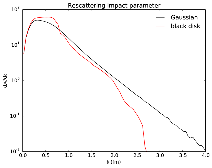
(a)

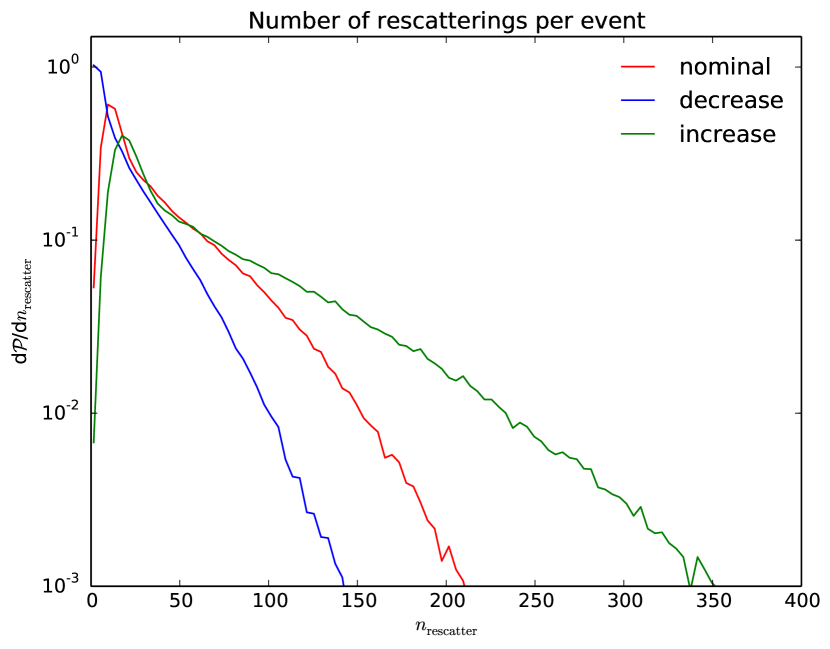
(b)

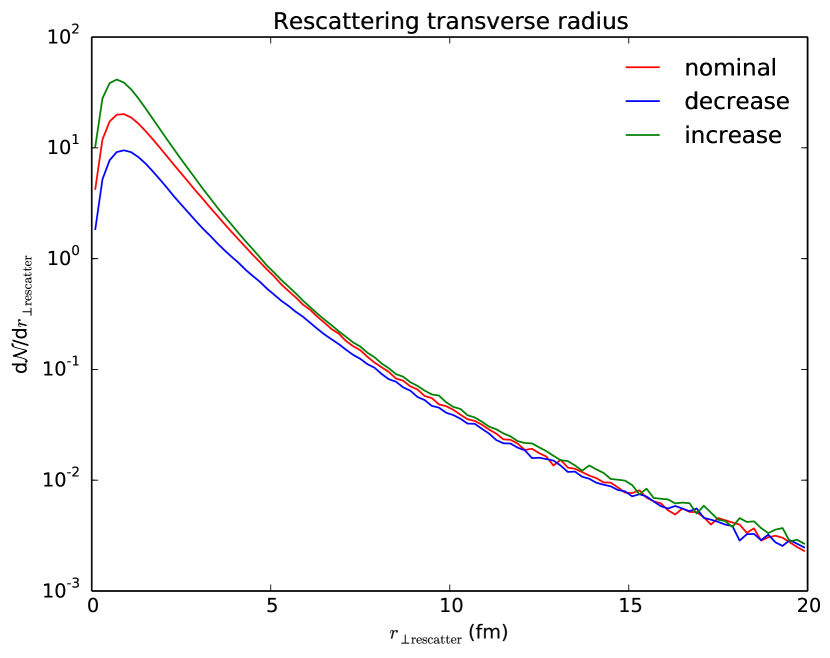
(c)

(d)

Figure 14: (a) The impact-parameter distribution of rescatterings for the different impact models. (b) Number of rescatterings per event. (c,d) Distribution of rescatterings in $r_{\perp}$ and $p_{\perp}$. Results are for 13 TeV nondiffractive $\mathrm{p}\mathrm{p}$ events.

As part of the new framework, several parameters and settings have been introduced. In this section, we study how changing these settings affects rescattering phenomenology. In particular, as a simple and direct test, we present how each main model setting impacts the average number of rescatterings per event. In addition to these new settings, we also study existing settings that could have an effect on rescattering. A summary of settings and their overall effects is given in Table 8, with the average number of rescatterings for different variations shown in Table 9. In more detail, the effect of the settings are as follows:

• Rescattering:impactModel describes how the rescattering probability depends on the impact parameter $b$. The default (1) is a Gaussian fall-off, while the alternative (0) is a sharp edge, see eqs.  (8) and (10). In a uniform medium the two alternatives are normalized to result in equal rescattering rates, as given by the cross section. In practice we see that the Gaussian option gives more long-range interactions, Figure 14a, as expected, but overall a somewhat reduced rescattering rate. This is because the particle density falls off from the central collision axis, such that there are fewer pairs at large than at small impact parameter to begin with. The fact that the Gaussian option gives a lower rescattering rate means that the loss of events in the important 0.3–0.7 fm region for the Gaussian model is not compensated for by including longer-range interactions.

• Rescattering:opacity is the rescattering probability at $b=0$, i.e. $P_{0}$ of eqs.  (8) and (10). A lower opacity reduces the probability of close interactions, but increases the range of interactions. This gives fewer rescatterings, for the same reason as above.

• Rescattering:quickCheck enables a simple check that tests whether two hadrons are moving away from each other at their respective time of creation in the CM frame of the event, and if so does not study further whether a rescattering is possible. This is faster than the more time-consuming full check, where the hadron pair is boosted to their common rest frame and the earliest particle is offset to a common time of creation before checking whether the hadrons move away from each other. Performing the quick check first reduces the total execution time by about a factor of two, since the number of hadron pairs to consider in an LHC event may be of the order of 10 000, whereof the vast majority are moving away from each other by any criterion (note that the full check is still performed on pairs that pass the simple check). The simple check rejects about 5% of the collisions that would have been accepted by the full check, but these false rejections typically are close to the (unphysically sharp) accept/reject border, and do not make a significant impact on rescattering distributions. For these reasons the quick check is on by default.

• Rescattering:nearestNeighbours allows hadrons that are produced as nearest neighbours along a string to rescatter against each other, see Section 2.3. The number of rescatterings goes up when on, but net effects do not change in proportion, since nearest-neighbour pairs are more likely to move in the same direction anyway.

• Rescattering:delayRegeneration and Rescattering:tauRegeneration are based on the assumption that it takes some formation time for a scattered hadron to build up a new wave function, and that during that time it has a reduced likelihood to scatter again. If delayRegeneration is switched on, this time is chosen at random according to an exponential distribution with average proper time (in fm) given by the tauRegeneration. Hadrons produced from string fragmentation are not affected, since they get their time offset from the hadronization process itself, roughly corresponding to an average $\tau$ of 1.5 fm. Setting $\tau_{\mathrm{regen}}=1$ fm reduces the number of rescatterings by about 10% relative to an instantaneous regeneration. The effect seems to saturate however, and increasing it to 2 fm does not make much further difference.

• HadronVertex:mode defines where the hadron vertex is placed in string hadronization. By default, hadrons are defined to be produced at the average location of the two string breaks that define it (see Figure 1). By setting HadronVertex:mode = 1, the production vertex is shifted forward in time to the point where the two colour endpoints meet for the first time, and setting it to $-1$ shifts it backwards in time by that same amount. These variations have a significant effect on the density of primary produced hadrons, changing the number of rescatterings by about 50%. For this reason we do not vary this setting in our studies, but instead use HadronVertex:kappa, which gives similar but milder effects, as explained below.

• HadronVertex:kappa is the string tension, by default $\kappa\approx 1$ GeV/fm, eq. (1). Increasing $\kappa$ compresses the production vertices and thus gives more rescattering. While the concept of a string tension is central in the hadronization framework, its exact value has not been relevant for the energy–momentum-related properties of an event. We allow for a generous $\pm$20% variation to also cover some uncertainty in how to define the hadron production vertex, as described above.

• HadronVertex:xySmear is the width of a Gaussian smearing of string breakup vertices in the plane perpendicular to the string, see Section 2.2. Increasing this slightly increases the transverse offsets of the primary produced hadron vertices, but does not have significant overall effects on rescattering.

• PartonVertex:modeVertex picks the shape of the overlap region between the two incoming protons, as used to pick the location of MPI vertices, see Section 2.2. Different shapes give some variation in rescattering features, but they are small ones for most properties, and it is hard to quantify the difference between the various shapes. For this reason, we do not vary this setting in subsequent model tests. It is however a way to introduce spatial anisotropy in the primary hadron distribution, which is necessary for azimuthal flow.

• PartonVertex:ProtonRadius is the three-dimensional proton radius, which then gets converted to a two-dimensional one for the distribution of MPI production vertices, eq. (3). Increasing/reducing this by 0.15 fm will increase/reduce the transverse radius of rescattering vertices by about 0.10 fm, and higher values give a slightly lower number of rescatterings.

• PartonVertex:EmissionWidth is the constant of proportionality for smearing of the transverse production vertices generated by partons showers, which are assumed to be inversely proportional to the $p_{\perp}$ of the parton. Varying this within a reasonable range has no significant effect on rescattering.

Setting	decrease	nominal	increase
Rescattering:impactModel	1	1	0
Rescattering:opacity	0.8	0.9	1.0
Rescattering:quickCheck	on	on	off
Rescattering:nearestNeighbours	off	on	on
Rescattering:tauRegeneration	2.	1.	0.
HadronVertex:kappa	0.8	1.	1.2
PartonVertex:ProtonRadius	1.0	0.85	0.7
MultipartonInteractions:pT0Ref	2.305	2.345	2.385

Table 10: List of model settings used to explore the range of possible rescattering effects. Here “increase” and “decrease” denote alternatives with more or less amount of rescattering relative to the default “nominal” values.

For comparison purposes, one nominal scenario is defined as our best assumption on relevant settings, and in addition two extremes with decreased or increased rescattering rate, Table 10. For each case, pT0Ref has been tuned as shown in the table in order to restore charged multiplicity.

The resulting variations of rescattering rates are shown in Figure 14b. The rate difference mainly arises around small transverse radii, Figure 14c (and early invariant times, not shown). By contrast, in properties such as the transverse momentum, Figure 14d, or invariant mass of the collision systems (not shown), the variations more affect the normalization than the shape of the distributions. Comparisons to data will be given in Section 5.2.

5 Comparison with data

While the standard Pythia generally gives a good description of LHC $\mathrm{p}\mathrm{p}$ data, there are some well-known discrepancies. One such is the shape of low-$p_{\perp}$ spectra of pions, Kaons and protons. Especially the poor description of the pion spectrum for $p_{\perp}<0.5$ GeV has direct consequences for a number of other distributions [64], e.g. when the pseudorapidity spectrum is studied either for $p_{\perp}>0.1$ GeV or $p_{\perp}>0.5$ GeV charged particles. In this section, we study how these spectra are changed by rescattering, using Rivet [65] to generate plots and comparisons to data. Results are shown initially for the default rescattering model, then for alternative parameter choices within this model, and eventually for model variations of the primary hadron production. Finally, we briefly consider the $p_{\perp}$ spectrum for the $\Lambda^{0}/\mathrm{K}_{S}^{0}$ ratio. As before, the pT0Ref parameter is retuned to ensure the same charged multiplicity in all scenarios studied.

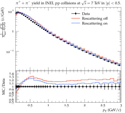
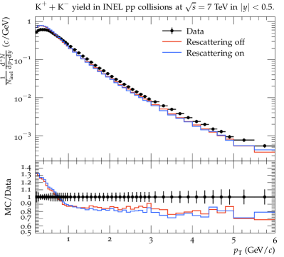
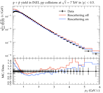
Figure 15: $p_{\perp}$ spectra for $\pi^{\pm}$, $\mathrm{K}^{\pm}$ and $\mathrm{p}/\overline{\mathrm{p}}$, compared with data from ALICE [8, 4].

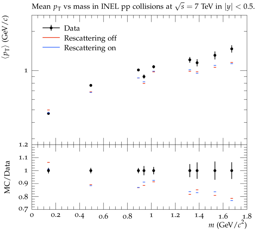
(a)

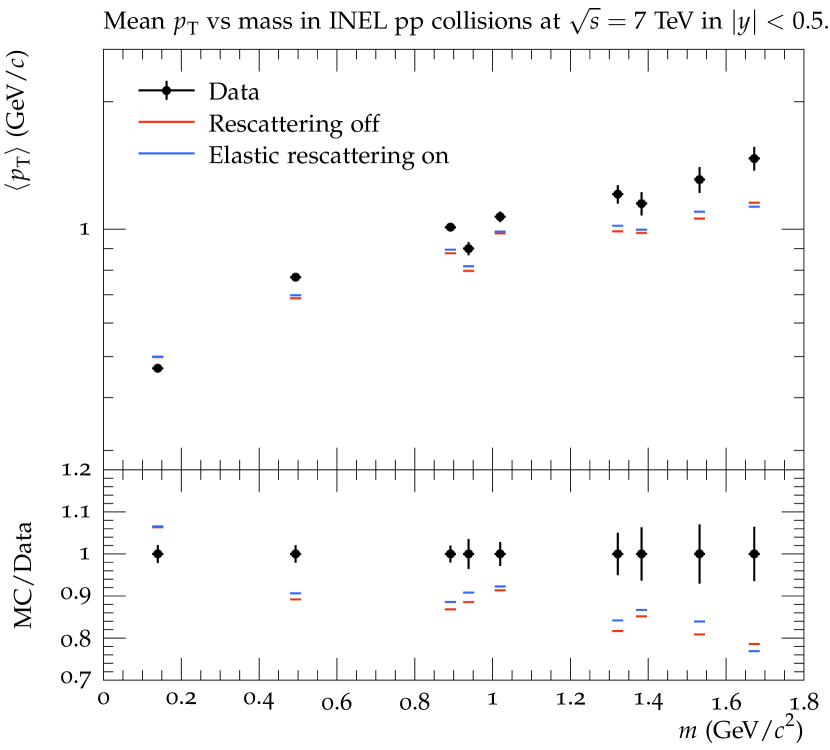
(b)

Figure 16: Average $p_{\perp}$ for different particle species, ordered by mass, with data from ALICE [8, 4]. The included particles are $\pi^{\pm}$, $\mathrm{K}^{\pm}$, $\mathrm{K}^{*}(892)^{\pm}$, $\mathrm{p}$, $\phi(1020)$, $\Xi^{-}$, $\Sigma^{*}(1385)^{\pm}$, $\Xi^{*}(1530)^{0}$ and $\Omega^{-}$. (a) Comparison of rescattering to no rescattering. (b) Comparison between the two when all rescatterings are forced to be elastic. Here we use the default pT0Ref = 2.28, since elastic scattering does not change charged multiplicity.

5.1 The effects of rescattering on transverse momentum speectra

Figure 15 shows the $p_{\perp}$ spectra for pions, Kaons and protons, with and without rescattering. We see that rescattering gives a better fit to data for pions and protons, especially at low $p_{\perp}$, while for Kaons rescattering moves the $p_{\perp}$ spectrum away from data. The average $p_{\perp}$ for various particle species is shown in Figure 16a, and here again there is an improvement for $\pi$ and $\mathrm{p}$, but a slight deterioration for $\mathrm{K}$.

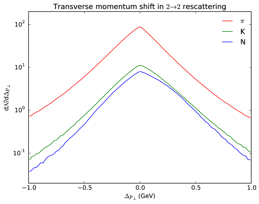
(a)

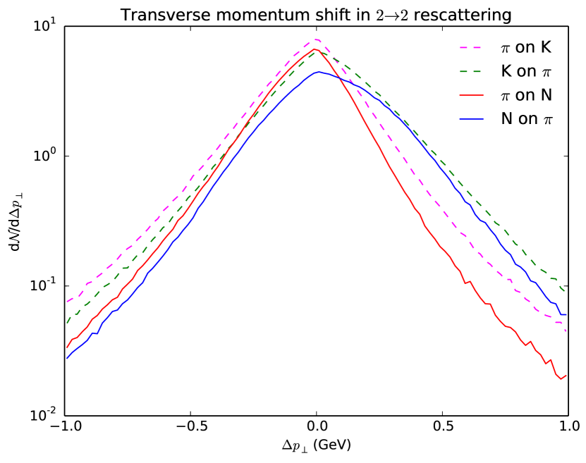
(b)

Figure 17: Shift of transverse momentum by $2\to 2$ elastic or resonant processes, where positive numbers correspond to an increased $p_{\perp}$ in the collision. (a) Inclusive shifts for $\pi$, $\mathrm{K}$ and $\mathrm{N}$ (including antiparticles). (b) Shifts in $\mathrm{K}\pi\to\mathrm{K}\pi$ and $\mathrm{N}\pi\to\mathrm{N}\pi$ scatterings.

If we consider only elastic collisions, one would expect that rescattering should push lighter particles towards lower $p_{\perp}$ and heavier particles to higher $p_{\perp}$. This is because lighter particles generally move faster and will catch up with and push the heavier ones outwards, a phenomenon sometimes referred to as “pion wind”. The actual momentum shifts in elastic rescatterings (including through resonances) is shown in Figure 17. Here we see a positive shift both for $\mathrm{K}$ and $\mathrm{N}$. This becomes more apparent if one considers only $\mathrm{K}\pi\to\mathrm{K}\pi$ and $\mathrm{N}\pi\to\mathrm{N}\pi$ scatterings, Figure 17b, where the heavier $\mathrm{K}/\mathrm{N}$ on the average gains $p_{\perp}$ at the expense of the lighter $\pi$. A closer study reveals that the strongest $p_{\perp}$ shifts comes from resonance production, i.e. $\mathrm{K}^{*}$ and $\Delta$ intermediate states. There are two reasons for this. Firstly, these resonances give large cross sections in a mass range where the flux of colliding pairs is large in the first place, and thus dominate over elastic scattering (in the processes discussed here). Secondly, elastic scattering is peaked in the forward direction, i.e. at small momentum transfers, while an $s$-channel spin 0 resonance decays isotropically in its rest frame.

In Figure 16b, we look at $\left<p_{\perp}\right>$ shifts when only elastic scattering is permitted. Specifically, this is done by calculating each total cross section as before, but setting the elastic cross section equal to the total one (thus excluding elastic scattering through a resonance). In this case, the $\langle p_{\perp}\rangle$ increases for all heavy particles except for $\Omega$, which is so rare so this can simply be explained by statistical fluctuations. For particles such as $\mathrm{p}$ and $\Sigma$, the change in $\left<p_{\perp}\right>$ is less than before, highlighting the fact that elastic scattering through a resonance gives the strongest momentum transfers. (As a side note, an unexpected observation is that the average pion $p_{\perp}$ actually increases very slightly, which turns out to be a consequence of the narrow rapidity window $|y|<0.5$ used in the experimental analysis; the average does decrease if all rapidities are included.)

So why then is the mean $p_{\perp}$ reduced for Kaons when inelastic interactions are allowed? The answer is that in processes classified as inelastic, especially non-diffractive processes, we make a significant effort to ensure that at least three particles are produced, so as to avoid the elastic channel. Such interactions have to share the $p_{\perp}$ between more outgoing than incoming particles, which leads to a reduced average. In principle, the opposite kind of interactions would be possible, where three (or more) incoming particles could fuse to give two outgoing ones, presumably then with an increased $p_{\perp}$. We have not implemented these kinds of processes in the first version of our framework, but their potential effect on the Kaon $p_{\perp}$ spectrum should make them a priority in future work.

Another observation from Figure 16a is that the mean $p_{\perp}$ of $\Sigma^{*}$ is also reduced. In addition to the aforementioned effect of $2\to n$ scattering, we have also observed that resonances formed during rescattering tend to have a lower $p_{\perp}$ than those produced directly from string fragmentation. From phase space considerations, it is less likely for two random high-$p_{\perp}$ particles to have an invariant mass in the resonance range than for two low-$p_{\perp}$ ones. The effect is especially large where the mass difference between the resonance and the particles forming it is small, such as for the $\Sigma^{*}$ baryons. These particles still tend to gain $p_{\perp}$ when they themselves participate in rescattering, as we see in Figure 16b.

(a)

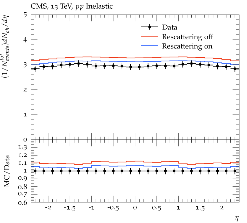
(b)

Figure 18: $p_{\perp}$ and $\eta$ spectra compared with data from CMS [66]. Charged particles with $p_{\perp}>500$ MeV and $|\eta|<2.4$ are considered.

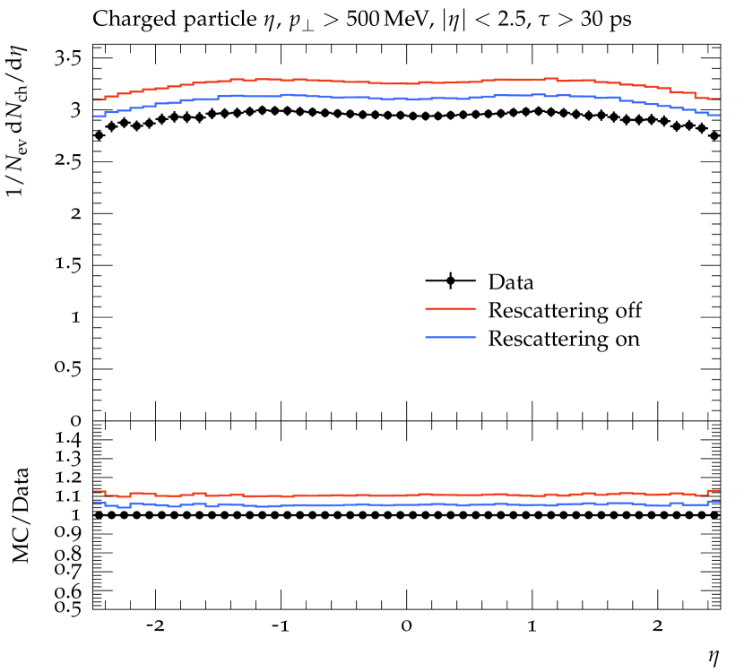
(a)

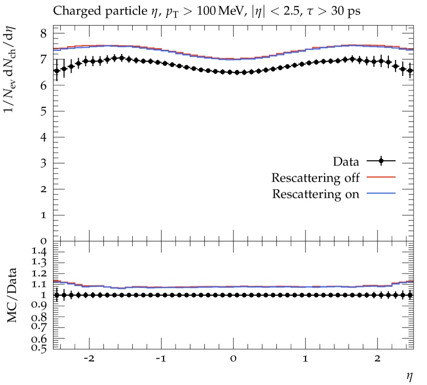
(b)

Figure 19: Charged particle $\eta$ spectra compared with data from ATLAS [67, 68], with cuts (a) $p_{\perp}>500$ MeV, and (b) $p_{\perp}>100$ MeV.

The total $p_{\perp}$ spectrum for all charged particles is shown in Figure 18a, and is improved overall by rescattering. The charged-particle pseudorapidity spectra in Figure 18b and 19a show that when a cut $p_{\perp}>500$ MeV is used, rescattering shifts the spectrum down by an approximately fixed amount, to a better agreement with data. However, this improvement is not visible in Figure 18b, where the cut is $p_{\perp}>100$ MeV. This suggests that the “true” pseudorapidity spectra are mostly unaffected by rescattering, but because of $p_{\perp}$ shifts, rescattering has an indirect effect on the observed spectrum. The takeaway from this is that data affected by low-$p_{\perp}$ particle production are likely to be better described when rescattering is included.

In summary, rescattering does what it is expected to in elastic scattering, i.e. slows down lighter hadrons and speeds up heavier ones. The disappointing aspect is that we have observed other mechanisms that work in the other direction. Finding ways to compensate for these effects should be addressed in future work.

5.2 Model dependence of transverse momentum spectra

Given the central role of the $p_{\perp}$ spectra, it is highly relevant to understand how sensitive they are to rescattering model variations. To this end, we can compare the default rescattering scenario with the two alternatives listed in Table 10. These two are selected to minimize or maximize the number of rescatterings, within reasonable extremes for each relevant setting.

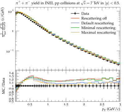
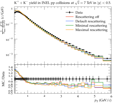
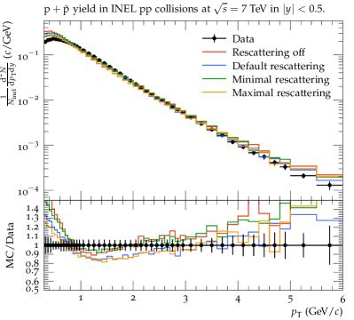
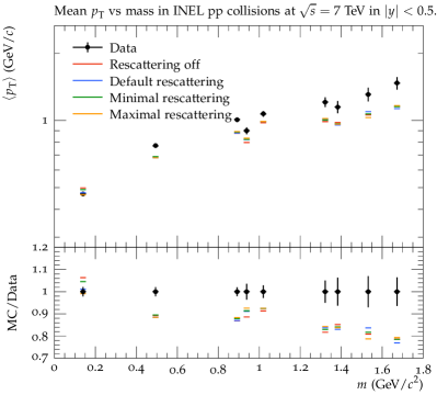
Figure 20: $p_{\perp}$ spectra for $\pi^{\pm}$, $\mathrm{K}^{\pm}$ and $\mathrm{p}/\overline{\mathrm{p}}$ and average $p_{\perp}$ for various particles, for different parameter configurations.

The results are shown in Figure 20. What we observe is that the effects on the $p_{\perp}$ spectra tend to scale with the amount of rescattering. This is especially clear for $\pi$ and $\mathrm{p}$, where the minimum/maximum amount of rescattering give smaller/larger effects than the default values, respectively. At the same time, the maximum setup gives a relatively small further improvement over the default rescattering one. It is therefore meaningful to stay with the default scenario, rather than trying to use more extreme choices to come closer to data.

5.3 The thermal model alternative

The rate of $\mathrm{q}\overline{\mathrm{q}}$ string breaks is traditionally assumed to involve a suppression factor $e^{-\pi m_{\perp\mathrm{q}}^{2}/\kappa}$: since the string does not contain any local concentrations of mass, a quark needs to tunnel out as a virtual particle until it has “eaten up” enough string length to correspond to its transverse mass [19]. This gives a Gaussian $p_{\perp}$ spectrum to quarks and, by addition, to hadrons. The derivation is done for a single string in isolation, however, whereas the reality at hadron colliders is that the typical event contains several more-or-less overlapping strings. This may modify the primary particle production processes, which set the starting stage for the continued rescattering and decay processes we have considered in this article. Empirically, an exponential spectrum $\exp(-m_{\perp\mathrm{had}}/T)$ was early on proposed as a parameterization of hadron collision data, where $m_{\perp\mathrm{had}}$ is the transverse hadron mass and $T$ could be associated with a temperature e.g. in the Hagedorn approach [69, 70, 71]. Interestingly, an effectively exponential fall-off could arise also starting from the Gaussian one, by assuming that the string tension is fluctuating along the string length, also in the absence of other strings [72].

Based on such ideas, a “thermal model” option has been included as an alternative in Pythia [16]. Unlike purely statistical models, however, it is strictly based on the string model, with local flavour and $p_{\perp}$ conservation. To this end, each $\mathrm{q}\overline{\mathrm{q}}$ breakup is associated with a (modified Bessel) $p_{\perp}$ distribution such that the two-dimensional convolution results in an $\exp(-p_{\perp\mathrm{had}}/T)$ spectrum. In each fragmentation step, an old $\mathrm{q}$ flavour is always known when the new one is selected and a new hadron is formed out of the two. Each new quark and hadron possibility is assigned a relative weight $\exp(-m_{\perp\mathrm{had}}/T)$, times relevant spin and symmetry factors, and these weights are used to make the random choice. The relative rate of diquark/baryon production requires a free parameter, while an additional $\mathrm{s}$-quark suppression factor is needed to achieve better agreement with observed production rates. The suppression of multistrange hadrons is underestimated, however, whereas the standard string model overestimates it, suggesting that “the truth” may lie somewhere in between.

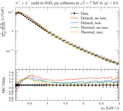
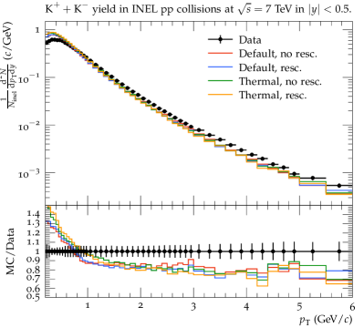
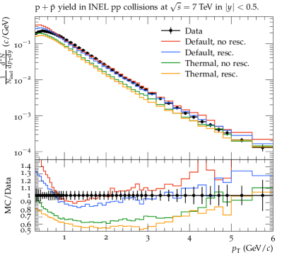
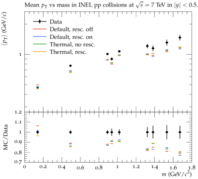
Figure 21: $p_{\perp}$ spectra for $\pi^{\pm}$, $\mathrm{K}^{\pm}$ and $\mathrm{p}/\overline{\mathrm{p}}$ and average $p_{\perp}$ for various particles, with comparing the Gaussian to the thermal model. When using the thermal model, pT0Ref has been tuned to 2.47 without rescattering and 2.52 with rescattering on, in order to maintain the correct $n_{\mathrm{charged}}$.

A key aspect of the $\exp(-m_{\perp\mathrm{had}}/T)$ weight is that heavier primary hadrons obtain a larger $\langle p_{\perp}\rangle$ than lighter ones. While it does enhance low-$p_{\perp}$ pion production and deplete ditto baryon one, relative to the traditional string model, the effects are not large enough to explain the data [16]. It is therefore interesting to combine the thermal model with rescattering, to check whether the two together give a larger combined improvement than each individually. The results of this comparison are shown in Figure 21, where the Gaussian model is compared to the thermal model, both with and without rescattering. The effects of the thermal model are similar to the effects of rescattering, with an improvement for the mean $p_{\perp}$ of pions and protons and a deterioration for Kaons. For pions, the correction from the combination of the two in fact overshoots the $\langle p_{\perp}\rangle$ data, so that either of them individually gives a better result than the two combined, even if the pion $p_{\perp}$ spectrum itself looks rather reasonable. We also see that the $p_{\perp}$ spectrum for protons is less accurate, especially at higher $p_{\perp}$s. For these reasons, the results of using the thermal model are not particularly encouraging, at least not without a more thorough retuning.

5.4 Close-packing

Apart from the possibility of a randomly fluctuating string tension, one may also expect systematic effects on the tension in a denser string environment, which can be modelled in different ways. One option implemented in Pythia is that of colour ropes [14], wherein several more-or-less parallel strings can fuse into a “rope”. The combined colour charge of this rope, as given by the Casimir operator, then gives a scaling-up factor applied to the string tension. When the rope breaks, the difference in charge before and after the break gives the effective charge involved in that $\mathrm{q}\overline{\mathrm{q}}$ production step. The other option is based on the assumption that a close-packing of strings gives them a smaller transverse area each, but preserves their separate identities [16]. Also in this option the string tension is increased, but in principle as a smooth function of the amount of squeezing rather than in the discrete steps of the rope. In practice, there need not be any big difference between these two options, but in this study we choose the second one for simplicity.

In this model, the creation of a new hadron is begun by an exploratory step ahead, so that the number of strings overlapping the rapidity range of the intended next hadron can be estimated. This local string number is then raised to some (tuned) power to give a rescaling factor for the string tension. To this basic picture some damping is introduced for particle production at large $p_{\perp}$, which typically occurs at larger transverse radii, away from the denser region. Note that the current implementation predates the introduction of space–time coordinates for the hadronization process, such that there now is room for improvements, but not ones that are likely to give a qualitatively changed behaviour for the properties studied here.

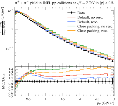
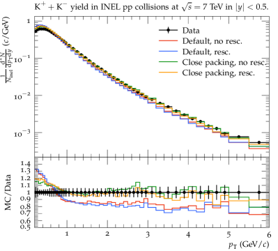
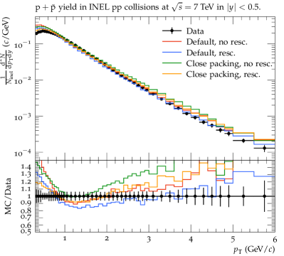
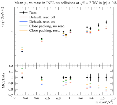
Figure 22: $p_{\perp}$ spectra for $\pi^{\pm}$, $\mathrm{K}^{\pm}$ and $\mathrm{p}/\overline{\mathrm{p}}$ and average $p_{\perp}$ for various particles, for the Gaussian model with and without close-packing corrections. When using the close-packing corrections, pT0Ref has been tuned to 2.18 without rescattering and 2.25 with rescattering on, in order to restore the correct $n_{\mathrm{charged}}$.

The close-packing modification can be used either for the standard string model or for the thermal alternative, by a rescaling either of $\kappa$ or of $T$. In Figure 22, we have used the former one. The trend here is that close-packing tends to increase $p_{\perp}$ for all particles, which means an improvement for all heavier hadrons, especially Kaons whose $p_{\perp}$ spectrum now follows data remarkably well above 1 GeV. However, this also means that the spectrum is worsened pions, and looking at their spectrum, the effect is quite severe. This deterioration is partially compensated for by rescattering, but not completely. This makes the close-packing option unsuited as it stands. A retuning of fragmentation parameters might ameliorate the situation, but that is beyond the scope of the current study.

5.5 The role of vector mesons

One of the standard assumptions is that the $p_{\perp}$ spectrum in $\mathrm{q}\overline{\mathrm{q}}$ string breaks is the same, independent of the quark species. This needs not be the case, and higher-order corrections could well favour slightly different $p_{\perp}$ values for strange quarks [73, 74], but for now we assume it to hold. Similarly, primary pseudoscalar and vector mesons are assumed to have the same $p_{\perp}$ spectra. The correct relative fraction of the two kinds of mesons is not known a priori, however, and for many hadrons it is difficult to measure their production rates, especially those with large widths. The prime example is the $\rho$, which we have seen contributes non-negligibly to the total rescattering rate. Since the $\rho$ has a higher mass than the Kaon, elastic $\rho\mathrm{K}$ collisions would tend to reduce the Kaon $p_{\perp}$, partially counteracting the gain from $\mathrm{K}\pi$ collisions.

As a simple test of the significance of heavy primary hadrons, we have studied a toy scenario where no vector mesons at all are produced in the primary string fragmentation, but still can occur as intermediate states during rescattering. The resulting $p_{\perp}$ spectra are shown in Figure 23. No attempt at a complete retune has been made, so it is the change by rescattering that is most interesting, not the overall agreement. Not unexpectedly, the $\langle p_{\perp}\rangle$ is wildly off for $K^{*}(892)$ and $\phi(1020)$, which now cannot be produced in the primary process. The “pion wind” effect is still there, in that rescattering shifts pions to smaller $p_{\perp}$ and protons to larger. For Kaons the $\langle p_{\perp}\rangle$ is still decreased by rescattering, providing further support that the primary mechanism for the Kaon $p_{\perp}$ loss is through $2\to n$ processes, rather than from Kaon collisions with heavier particles.

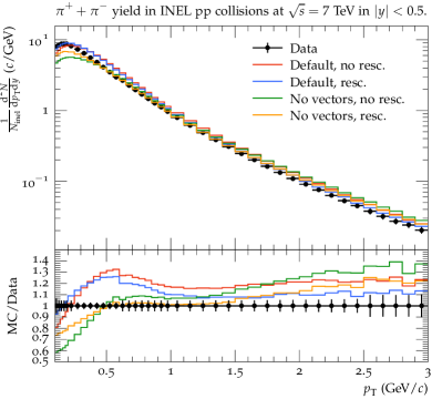
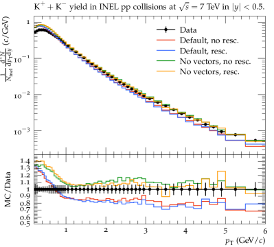
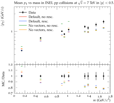
Figure 23: $p_{\perp}$ spectra for $\pi^{\pm}$, $\mathrm{K}^{\pm}$ and $\mathrm{p}/\overline{\mathrm{p}}$ and average $p_{\perp}$ for various particles, comparing rescattering to no rescattering, when no vector mesons are produced in the primary hadronization.

It could have been informative also to go in the other direction, and include primary production of higher resonances, with orbital or radial excitations. Measurements at LEP show that such mesons are produced at a non-negligible rate [46]. And yet, their explicit inclusion tend to reduce the goodness of fit to many other properties, presumably because the assumed isotropic decay distributions do not represent the correct physics. Instead a higher-mass state could be viewed as a longer-than-normal string piece, with a decay along this string direction, just as if these products come directly from the string. Therefore we do not expect primary production of higher resonances to change $p_{\perp}$ properties appreciably, but currently do not have the full machinery necessary to test this assumption.

5.6 Other transverse momentum spectra

So far we have focused on $p_{\perp}$ spectra for pions, Kaons and protons. However, another experimental observation that pertains to collective behaviour is the peak for example in the $\Lambda^{0}/\mathrm{K}^{0}_{S}$ ratio around $p_{\perp}\approx 2$ GeV. In Figure 24, the ratios for $\Lambda^{0}/\mathrm{K}^{0}_{S}$ and $\Xi^{-}/\Lambda^{0}$ are shown. Unfortunately rescattering does not provide an improvement. If anything it causes a deterioration, by reducing the relative number of $\Lambda^{0}$ and $\Xi^{-}$ baryons through the baryon-antibaryon annihilation mechanism. As before, an inclusion of $3\to 2$ processes could help alleviate the problem, but hardly give full agreement. In general, baryon production has been one of the more complicated and least successful aspects of the string fragmentation framework, already in the simpler $\mathrm{e}^{+}\mathrm{e}^{-}$ environment, and remains so.

(a)

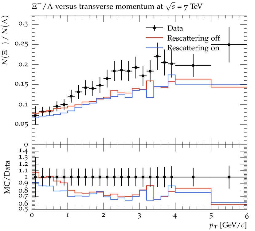
(b)

Figure 24: $p_{\perp}$ ratios of (a) $\Lambda^{0}$ to $\mathrm{K}_{\mathrm{S}}$ and (b) $\Xi^{-}$ to $\Lambda^{0}$.

6 Summary and Outlook

Hadronic rescattering is inevitable in the dense hadronic systems produced in high-energy $\mathrm{p}\mathrm{p}$ collisions. What less understood is the rate at which it happens, and the detailed modelling of the processes involved is open to discussion.

In this article we have developed and studied a framework for hadronic rescattering in $\mathrm{p}\mathrm{p}$ collisions. This involves three main aspects:

1. The space–time tracing of the motion of hadrons, with interleaved scatterings and decays. The starting point here is our picture for the space–time production of hadrons. Thereafter the motion of these hadrons is traced and possible crossings identified. The technical challenge is the fast growth of the number of hadron pairs to check, which can make have a significant impact on computing speed, even though most of these pairs never interact.

2. The cross section for different collision processes. This is where most of the development effort has gone, and most of the new code can be found. Much of the input has been from external sources, such as UrQMD ansätze, the calculations by Peláez et al., the HPR₁R₂, CERN/HERA and SaS parameterizations, and experimental data. We have tried to combine and extend these parts sensibly. For hadron pairs not described in any other way, the Additive Quark Model is invoked to provide order-of-magnitude cross sections, also for charm and bottom hadrons.

3. The production of the new hadrons in these collisions. This is done either through explicit few-body channels, like elastic scattering or resonance formation, or through the existing string fragmentation machinery. The typical collisions energies are so small, however, that extra efforts have to be made to translate these tiny strings into acceptable final states.

Each of the three components are open to further refinements, but the new framework presented here should offer a good starting point for various studies as is. Other frameworks overlapping with ours already exist. To the extent feasible, one obvious future task would be to compare with other rescattering implementations, starting from the same initial hadron configuration.

Nevertheless, what we bring now is a cohesive implementation, where the full power of the traditional Pythia energy–momentum description is extended by the recent matching space–time picture and the new rescattering components, without the need to bridge disparate codes. This framework can then be applied to $\mathrm{p}\mathrm{p}$ collisions of any kind, from minimum-bias to high-$p_{\perp}$ physics. As far as we know, no other single program can offer as much.

The main emphasis in this study has been to develop and test the framework, and to explore and understand how it behaves in general terms. Some applications to LHC $\mathrm{p}\mathrm{p}$ studies have also been presented. In particular we note that rescattering contributes to some aspects of collective flow, notably a “pion wind” that slows down pions and speeds up protons and (most) other baryons. This helps remedy one of the glaring discrepancies of the traditional Pythia setup in comparisons with data. Unfortunately, the effects are not large enough to fully resolve the discrepancies. Worse, the Kaon $p_{\perp}$ spectrum is not modified appreciably, owing to a balance between speedup from the pion wind and slowdown from $2\to n,n\geq 3$ processes. For this reason, one interesting topic for future study is the modelling of $3\to 2$ and related processes. There are also other phenomena, like azimuthal flow, where rescattering appears to give only a very small contribution.

Thus it is obvious that further mechanisms will be needed to reach agreement with a number of observables. We have here briefly explored some potential options, such as a randomly fluctuating string tension, i.e. the “thermal” model, and a larger string tension in a dense-string environment. Other ideas remain to be mixed in, such as string shoving. It may be disappointing not to be in a situation where one simple model describes it all, but the reality is that any physical process that can happen will also do so, at some level.

The framework and its individual components have a higher applicability than the one presented in this article, and we envisage several follow-up studies. The most obvious one is to step up from $\mathrm{p}\mathrm{p}$ to $\mathrm{p}$A and $\mathrm{A}\mathrm{A}$. This should be straightforward, since Pythia already contains the Angantyr framework for heavy-ion collisions [75]. In a first step, we would study the effects of rescattering on its own, without any other mechanisms for collective flow. In a second step, one could combine it with other effects, such as shove and rope formation, which also contribute to flow effects.

One relevant $\mathrm{A}\mathrm{A}$ study has already been done [32], based on Pythia/Angantyr and its space–time picture, but interfacing UrQMD to handle the rescattering. Physics comparisons between the two approaches will be useful on its own, but additionally we hope that we can offer a more user-friendly framework, thereby simplifying the future experimental study of rescattering effects.

Although this article has mainly focused on rescattering, it should not be overlooked that the underlying framework, which allows for collisions for different beam particles and collision energies from the mass threshold and upwards, has other potential use cases. It could for example come in handy for other applications, such as the simulation of cosmic ray showers in the atmosphere and of hadronic showers in detectors. Currently this flexibility only works for soft collisions, however. In order to fully include perturbative QCD aspects, such as jets and MPIs, it is necessary to specify meaningful PDFs for all colliding hadron species. Relevant combinations then have to be stored such that it is easy to switch between them. A special aspect is that, whereas collider physics mainly addresses particle production at central rapidities, the evolution of hadronic showers is especially sensitive to the production of the most forward hadrons, which therefore has to be carefully modelled.

In the current article, there has been no effort at a detailed retuning of all model parameters, but only a modest revision of $p_{\perp 0}$ to retain the same total charged multiplicity as before when rescattering is switched on. A future exercise would be to do a full-fledged retuning. This could start with $\mathrm{e}^{+}\mathrm{e}^{-}$ annihilation events at LEP, where no big effects are expected. Even small ones would be of interest, however, since they could also add one more source of uncertainty in $\mathrm{W}$ mass determinations [76], in addition to colour reconnection [77] and Bose-Einstein [78].

In conclusion, we hope that the current article and the new Pythia capabilities will be interesting for the experimental community, and also open up for further developments and studies. By experience we know that new generator capabilities tend to inspire both expected and unexpected applications.

References

- [1] CMS Collaboration, V. Khachatryan et al., “Observation of Long-Range Near-Side Angular Correlations in Proton-Proton Collisions at the LHC,” JHEP 09 (2010) 091, arXiv:1009.4122 [hep-ex].
- [2] ATLAS Collaboration, G. Aad et al., “Observation of Long-Range Elliptic Azimuthal Anisotropies in 13 and 2.76 TeV Collisions with the ATLAS Detector,” Phys. Rev. Lett. 116 no. 17, (2016) 172301, arXiv:1509.04776 [hep-ex].
- [3] CMS Collaboration, V. Khachatryan et al., “Evidence for collectivity in pp collisions at the LHC,” Phys. Lett. B765 (2017) 193–220, arXiv:1606.06198 [nucl-ex].
- [4] ALICE Collaboration, J. Adam et al., “Measurement of pion, kaon and proton production in proton-proton collisions at TeV,” Eur. Phys. J. C75 no. 5, (2015) 226, arXiv:1504.00024 [nucl-ex].
- [5] ALICE Collaboration, J. Adam et al., “Enhanced production of multi-strange hadrons in high-multiplicity proton-proton collisions,” Nature Phys. 13 (2017) 535–539, arXiv:1606.07424 [nucl-ex].
- [6] ALICE Collaboration, S. Acharya et al., “Investigations of Anisotropic Flow Using Multiparticle Azimuthal Correlations in pp, p-Pb, Xe-Xe, and Pb-Pb Collisions at the LHC,” Phys. Rev. Lett. 123 no. 14, (2019) 142301, arXiv:1903.01790 [nucl-ex].
- [7] CMS Collaboration, V. Khachatryan et al., “Strange Particle Production in Collisions at and 7 TeV,” JHEP 05 (2011) 064, arXiv:1102.4282 [hep-ex].
- [8] ALICE Collaboration, B. B. Abelev et al., “Production of and in proton-proton collisions at 7 TeV,” Eur. Phys. J. C75 no. 1, (2015) 1, arXiv:1406.3206 [nucl-ex].
- [9] J. Adolfsson et al., “QCD Challenges from pp to A-A Collisions,” 2020. arXiv:2003.10997 [hep-ph].
- [10] P. Braun-Munzinger and J. Stachel, “The quest for the quark-gluon plasma,” Nature 448 (2007) 302–309.
- [11] W. Busza, K. Rajagopal, and W. van der Schee, “Heavy Ion Collisions: The Big Picture, and the Big Questions,” Ann. Rev. Nucl. Part. Sci. 68 (2018) 339–376, arXiv:1802.04801 [hep-ph].
- [12] J. L. Nagle and W. A. Zajc, “Small System Collectivity in Relativistic Hadronic and Nuclear Collisions,” Ann. Rev. Nucl. Part. Sci. 68 (2018) 211–235, arXiv:1801.03477 [nucl-ex].
- [13] T. Pierog, I. Karpenko, J. M. Katzy, E. Yatsenko, and K. Werner, “EPOS LHC: Test of collective hadronization with data measured at the CERN Large Hadron Collider,” Phys. Rev. C92 no. 3, (2015) 034906, arXiv:1306.0121 [hep-ph].
- [14] C. Bierlich, G. Gustafson, L. Lönnblad, and A. Tarasov, “Effects of Overlapping Strings in pp Collisions,” JHEP 03 (2015) 148, arXiv:1412.6259 [hep-ph].
- [15] C. Bierlich, G. Gustafson, and L. Lönnblad, “A shoving model for collectivity in hadronic collisions,” arXiv:1612.05132 [hep-ph].
- [16] N. Fischer and T. Sjöstrand, “Thermodynamical String Fragmentation,” JHEP 01 (2017) 140, arXiv:1610.09818 [hep-ph].
- [17] T. Sjöstrand and M. van Zijl, “A Multiple Interaction Model for the Event Structure in Hadron Collisions,” Phys. Rev. D36 (1987) 2019.
- [18] T. Sjöstrand, “The Development of MPI Modeling in Pythia,” Adv. Ser. Direct. High Energy Phys. 29 (2018) 191–225, arXiv:1706.02166 [hep-ph].
- [19] B. Andersson, G. Gustafson, G. Ingelman, and T. Sjöstrand, “Parton Fragmentation and String Dynamics,” Phys. Rept. 97 (1983) 31–145.
- [20] S. Ferreres-Solé and T. Sjöstrand, “The space-time structure of hadronization in the Lund model,” Eur. Phys. J. C78 no. 11, (2018) 983, arXiv:1808.04619 [hep-ph].
- [21] M. Bähr et al., “Herwig++ Physics and Manual,” Eur. Phys. J. C58 (2008) 639–707, arXiv:0803.0883 [hep-ph].
- [22] J. Bellm et al., “Herwig 7.0/Herwig++ 3.0 release note,” Eur. Phys. J. C76 no. 4, (2016) 196, arXiv:1512.01178 [hep-ph].
- [23] T. Sjöstrand, S. Mrenna, and P. Z. Skands, “PYTHIA 6.4 Physics and Manual,” JHEP 05 (2006) 026, arXiv:hep-ph/0603175 [hep-ph].
- [24] T. Sjöstrand, S. Ask, J. R. Christiansen, R. Corke, N. Desai, P. Ilten, S. Mrenna, S. Prestel, C. O. Rasmussen, and P. Z. Skands, “An Introduction to PYTHIA 8.2,” Comput. Phys. Commun. 191 (2015) 159–177, arXiv:1410.3012 [hep-ph].
- [25] T. Gleisberg, S. Hoeche, F. Krauss, M. Schonherr, S. Schumann, F. Siegert, and J. Winter, “Event generation with SHERPA 1.1,” JHEP 02 (2009) 007, arXiv:0811.4622 [hep-ph].
- [26] E. Bothmann et al., “Event Generation with Sherpa 2.2,” SciPost Phys. 7 no. 3, (2019) 034, arXiv:1905.09127 [hep-ph].
- [27] Y.-X. Zhang et al., “Comparison of heavy-ion transport simulations: Collision integral in a box,” Phys. Rev. C97 no. 3, (2018) 034625, arXiv:1711.05950 [nucl-th].
- [28] S. A. Bass et al., “Microscopic models for ultrarelativistic heavy ion collisions,” Prog. Part. Nucl. Phys. 41 (1998) 255–369, arXiv:nucl-th/9803035 [nucl-th]. [Prog. Part. Nucl. Phys.41,225(1998)].
- [29] J. Weil et al., “Particle production and equilibrium properties within a new hadron transport approach for heavy-ion collisions,” Phys. Rev. C94 no. 5, (2016) 054905, arXiv:1606.06642 [nucl-th].
- [30] B. H. Sa and A. Tai, “An Event generator for the firecracker model and the rescattering in high-energy p A and A-A collisions: LUCIAE version 2.0,” Comput. Phys. Commun. 90 (1995) 121–140.
- [31] B.-H. Sa, D.-M. Zhou, Y.-L. Yan, X.-M. Li, S.-Q. Feng, B.-G. Dong, and X. Cai, “PACIAE 2.0: An Updated parton and hadron cascade model (program) for the relativistic nuclear collisions,” Comput. Phys. Commun. 183 (2012) 333–346, arXiv:1104.1238 [nucl-th].
- [32] A. V. da Silva, C. Bierlich, D. Dobrigkeit Chinellato, and J. Takahashi, “Studying the effect of the hadronic phase in nuclear collisions with PYTHIA and UrQMD,” in 18th International Conference on Strangeness in Quark Matter (SQM 2019) Bari, Italy, June 10-15, 2019. 2019. arXiv:1911.12824 [nucl-th].
- [33] G. ’t Hooft, “A Planar Diagram Theory for Strong Interactions,” Nucl. Phys. B72 (1974) 461.
- [34] T. Sjöstrand, “Jet Fragmentation of Nearby Partons,” Nucl. Phys. B248 (1984) 469–502.
- [35] K. Gallmeister and T. Falter, “Space-time picture of fragmentation in PYTHIA/JETSET for HERMES and RHIC,” Phys. Lett. B630 (2005) 40–48, arXiv:nucl-th/0502015 [nucl-th].
- [36] C. Bierlich and C. O. Rasmussen, “Dipole evolution: perspectives for collectivity and A collisions,” JHEP 10 (2019) 026, arXiv:1907.12871 [hep-ph].
- [37] A. H. Mueller, “Soft gluons in the infinite momentum wave function and the BFKL pomeron,” Nucl. Phys. B415 (1994) 373–385.
- [38] A. H. Mueller and B. Patel, “Single and double BFKL pomeron exchange and a dipole picture of high-energy hard processes,” Nucl. Phys. B425 (1994) 471–488, arXiv:hep-ph/9403256.
- [39] T. Sjöstrand and P. Z. Skands, “Multiple interactions and the structure of beam remnants,” JHEP 03 (2004) 053, hep-ph/0402078.
- [40] Z. Xu and C. Greiner, “Thermalization of gluons in ultrarelativistic heavy ion collisions by including three-body interactions in a parton cascade,” Phys. Rev. C71 (2005) 064901, arXiv:hep-ph/0406278 [hep-ph].
- [41] G. Peter, D. Behrens, and C. C. Noack, “Poincare covariant particle dynamics. 1: Intranuclear cascade model,” Phys. Rev. C49 (1994) 3253–3265.
- [42] D. Behrens, G. Peter, and C. C. Noack, “Poincare covariant particle dynamics. 2: Fragmentation for ultrarelativistic reactions,” Phys. Rev. C49 (1994) 3266–3274.
- [43] C. B. Duncan and P. Skands, “Fragmentation of Two Repelling QCD Strings,” arXiv:1912.09639 [hep-ph].
- [44] E. M. Levin and L. L. Frankfurt, “The Quark hypothesis and relations between cross-sections at high-energies,” JETP Lett. 2 (1965) 65–70.
- [45] H. J. Lipkin, “Quarks for pedestrians,” Phys. Rept. 8 (1973) 173–268.
- [46] Particle Data Group Collaboration, M. Tanabashi et al., “Review of Particle Physics,” Phys. Rev. D98 no. 3, (2018) 030001.
- [47] R. Garcia-Martin, R. Kaminski, J. R. Pelaez, J. Ruiz de Elvira, and F. J. Yndurain, “The Pion-pion scattering amplitude. IV: Improved analysis with once subtracted Roy-like equations up to 1100 MeV,” Phys. Rev. D83 (2011) 074004, arXiv:1102.2183 [hep-ph].
- [48] J. R. Pelaez, A. Rodas, and J. Ruiz De Elvira, “Global parameterization of scattering up to 2 ,” Eur. Phys. J. C79 no. 12, (2019) 1008, arXiv:1907.13162 [hep-ph].
- [49] J. Pelaez and A. Rodas, “Pion-kaon scattering amplitude constrained with forward dispersion relations up to 1.6 GeV,” Phys. Rev. D 93 no. 7, (2016) 074025, arXiv:1602.08404 [hep-ph].
- [50] V. Srinivasan et al., “Pi- pi+ –¿ pi- pi+ Interactions Below 0.7-GeV from pi- p –¿ pi- pi+ n Data at 5-GeV/c,” Phys. Rev. D12 (1975) 681.
- [51] S. D. Protopopescu, M. Alston-Garnjost, A. Barbaro-Galtieri, S. M. Flatte, J. H. Friedman, T. A. Lasinski, G. R. Lynch, M. S. Rabin, and F. T. Solmitz, “Pi pi Partial Wave Analysis from Reactions pi+ p —¿ pi+ pi- Delta++ and pi+ p —¿ K+ K- Delta++ at 7.1-GeV/c,” Phys. Rev. D7 (1973) 1279.
- [52] N. N. Biswas, N. M. Cason, I. Derado, V. P. Kenney, J. A. Poirier, and W. D. Shephard, “Total Pion-Pion Cross Sections for the 2-GeV Di-Pion Mass Region,” Phys. Rev. Lett. 18 no. 7, (1967) 273–276.
- [53] W. J. Robertson, W. D. Walker, and J. L. Davis, “High-energy pi pi collisions,” Phys. Rev. D7 (1973) 2554–2564.
- [54] Particle Data Group Collaboration, L. Montanet et al., “Review of particle properties. Particle Data Group,” Phys. Rev. D 50 (1994) 1173–1823.
- [55] A. Donnachie and P. V. Landshoff, “Dynamics of Elastic Scattering,” Nucl. Phys. B267 (1986) 690–701.
- [56] G. A. Schuler and T. Sjöstrand, “Hadronic diffractive cross-sections and the rise of the total cross-section,” Phys. Rev. D49 (1994) 2257–2267.
- [57] P. Koch and C. B. Dover, “, and Production in Relativistic Heavy Ion Collisions,” Phys. Rev. C40 (1989) 145–155.
- [58] G. A. Schuler and T. Sjöstrand, “A Scenario for high-energy gamma gamma interactions,” Z. Phys. C73 (1997) 677–688, arXiv:hep-ph/9605240 [hep-ph].
- [59] C. O. Rasmussen and T. Sjöstrand, “Models for total, elastic and diffractive cross sections,” Eur. Phys. J. C78 no. 6, (2018) 461, arXiv:1804.10373 [hep-ph].
- [60] S. Navin, “Diffraction in Pythia,” arXiv:1005.3894 [hep-ph].
- [61] P. Skands, S. Carrazza, and J. Rojo, “Tuning PYTHIA 8.1: the Monash 2013 Tune,” Eur. Phys. J. C74 no. 8, (2014) 3024, arXiv:1404.5630 [hep-ph].
- [62] T. Sjöstrand and P. Z. Skands, “Baryon number violation and string topologies,” Nucl. Phys. B659 (2003) 243, arXiv:hep-ph/0212264 [hep-ph].
- [63] M. Cacciari, G. P. Salam, and G. Soyez, “The anti- jet clustering algorithm,” JHEP 04 (2008) 063, arXiv:0802.1189 [hep-ph].
- [64] ATLAS Collaboration, G. Aad et al., “Charged-particle multiplicities in pp interactions measured with the ATLAS detector at the LHC,” New J. Phys. 13 (2011) 053033, arXiv:1012.5104 [hep-ex].
- [65] C. Bierlich et al., “Robust Independent Validation of Experiment and Theory: Rivet version 3,” SciPost Phys. 8 (2020) 026, arXiv:1912.05451 [hep-ph].
- [66] CMS Collaboration, A. M. Sirunyan et al., “Measurement of charged particle spectra in minimum-bias events from proton–proton collisions at ,” Eur. Phys. J. C 78 no. 9, (2018) 697, arXiv:1806.11245 [hep-ex].
- [67] ATLAS Collaboration, G. Aad et al., “Charged-particle distributions in = 13 TeV pp interactions measured with the ATLAS detector at the LHC,” Phys. Lett. B 758 (2016) 67–88, arXiv:1602.01633 [hep-ex].
- [68] ATLAS Collaboration, M. Aaboud et al., “Charged-particle distributions at low transverse momentum in TeV interactions measured with the ATLAS detector at the LHC,” Eur. Phys. J. C 76 no. 9, (2016) 502, arXiv:1606.01133 [hep-ex].
- [69] R. Hagedorn, “Statistical thermodynamics of strong interactions at high-energies,” Nuovo Cim. Suppl. 3 (1965) 147–186.
- [70] R. Hagedorn, “Remarks on the thermodynamical model of strong interactions,” Nucl. Phys. B24 (1970) 93–139.
- [71] R. Hagedorn, “Multiplicities, Distributions and the Expected Hadron Quark - Gluon Phase Transition,” Riv. Nuovo Cim. 6N10 (1983) 1–50.
- [72] A. Bialas, “Fluctuations of string tension and transverse mass distribution,” Phys. Lett. B 466 (1999) 301–304, arXiv:hep-ph/9909417.
- [73] A. Casher, H. Neuberger, and S. Nussinov, “Chromoelectric Flux Tube Model of Particle Production,” Phys. Rev. D 20 (1979) 179–188.
- [74] P. Skands, “Introduction to QCD,” in Theoretical Advanced Study Institute in Elementary Particle Physics: Searching for New Physics at Small and Large Scales, pp. 63–124. 2017. arXiv:1207.2389 [hep-ph].
- [75] C. Bierlich, G. Gustafson, L. Lönnblad, and H. Shah, “The Angantyr model for Heavy-Ion Collisions in PYTHIA8,” JHEP 10 (2018) 134, arXiv:1806.10820 [hep-ph].
- [76] ALEPH, DELPHI, L3, OPAL, LEP Electroweak Collaboration, S. Schael et al., “Electroweak Measurements in Electron-Positron Collisions at W-Boson-Pair Energies at LEP,” Phys.Rept. 532 (2013) 119–244, arXiv:1302.3415 [hep-ex].
- [77] T. Sjöstrand and V. A. Khoze, “On Color rearrangement in hadronic events,” Z. Phys. C62 (1994) 281–310, arXiv:hep-ph/9310242.
- [78] L. Lönnblad and T. Sjöstrand, “Modeling Bose-Einstein correlations at LEP-2,” Eur. Phys. J. C2 (1998) 165–180, arXiv:hep-ph/9711460 [hep-ph].