Primordial Black Holes Confront LIGO/Virgo data: Current situation

Abstract

The LIGO and Virgo Interferometers have so far provided 11 gravitational-wave (GW) observations of black-hole binaries. Similar detections are bound to become very frequent in the near future. With the current and upcoming wealth of data, it is possible to confront specific formation models with observations. We investigate here whether current data are compatible with the hypothesis that LIGO/Virgo black holes are of primordial origin. We compute in detail the mass and spin distributions of primordial black holes (PBHs), their merger rates, the stochastic background of unresolved coalescences, and confront them with current data from the first two observational runs, also including the recently discovered GW190412. We compute the best-fit values for the parameters of the PBH mass distribution at formation that are compatible with current GW data. In all cases, the maximum fraction of PBHs in dark matter is constrained by these observations to be $f_{\text{\tiny\rm PBH}}\approx{\rm few}\times 10^{-3}$. We discuss the predictions of the PBH scenario that can be directly tested as new data become available. In the most likely formation scenarios where PBHs are born with negligible spin, the fact that at least one of the components of GW190412 is moderately spinning is incompatible with a primordial origin for this event, unless accretion or hierarchical mergers are significant. In the absence of accretion, current non-GW constraints already exclude that LIGO/Virgo events are all of primordial origin, whereas in the presence of accretion the GW bounds on the PBH abundance are the most stringent ones in the relevant mass range. A strong phase of accretion during the cosmic history would favour mass ratios close to unity, and a redshift-dependent correlation between high masses, high spins and nearly-equal mass binaries, with the secondary component spinning faster than the primary. Finally, we highlight that accretion can play an important role to relax current constraints on the PBH abundance, which calls for a better modelling of the mass and angular momentum accretion rates at redshift $z\lesssim 30$.

1 Introduction

Thanks to the current available measurements of the Gravitational Waves (GWs) from Black Holes (BHs) mergers in the observational runs O1 and O2 [1] and the more recent ongoing third phase [2] by the LIGO/Virgo collaborations, we have entered the era of GW astronomy. One of the most fundamental questions such observations raise is the nature of the BHs [3]. One fascinating hypothesis is that the merging BHs are of primordial origin, that is, they have formed early in the evolution of the universe (see Ref. [4] for a recent review). This possibility is also interesting as Primordial Black Holes (PBHs) may comprise the totality or a fraction of the Dark Matter (DM) in the universe [5, 6].

In order to assess if the merger events may be ascribed to PBHs one needs to go through various steps:

1. First, one starts from a given mass function distribution (which might be theoretically justified by a given PBH formation mechanism). Such mass function is determined by a set of parameters (typically two of them) parametrising the characteristic PBH mass scale and the width of the distribution. Their central values may be estimated from observations by requiring that all GW events detected so far (or a fraction thereof) are explained by PBHs. This requires fitting the key observables, namely the merger rate, the BH masses, and the redshift at which the event is produced, resulting in the best-fit value for the PBH abundance $f_{\text{\tiny\rm PBH}}$ in units of the DM one.

2. Secondly, one has to check if the resulting model parameters and $f_{\text{\tiny\rm PBH}}$ are compatible with the current constraints from other observations (e.g. lensing and CMB distortion) [7]. This second step is necessary to check which fraction of the PBHs may form the DM and, above all, to see if the observed events are compatible with the PBH scenario, or if their primordial origin is already excluded by other observations.

3. Thirdly, one can confront the theoretical predictions obtained through the PBH hypothesis of some key quantities, e.g. the binary chirp masses, mass ratios, spins, with the observed values, thus assessing whether the predictions are compatible or in tension with observations.

The goal of this paper is to explore if the first two observational LIGO/Virgo runs – also including the event GW190412 recently discovered in O3 – are compatible with the hypothesis that the BHs are of primordial origin. In particular, we calculate the mass and spin distributions of PBHs, their merger rates, the stochastic background of unresolved coalescences, and confront them with current data.

One particularly relevant phenomenon to take into account when performing such analysis is PBH mass accretion. Indeed, PBHs may accrete efficiently during the cosmic history, see for instance [8, 9, 10]. First of all accretion changes the PBH masses, their mass functions, and their abundances. This is relevant when analysing the constraints at the present epoch for PBHs with masses larger than a few solar masses [11]. Furthermore, accretion may strongly influence the PBH merger rates, their final spins [12], as well as their mass ratios in the binaries. This is particularly important not only because the binary masses and effective spin parameter $\chi_{\text{\tiny eff}}$ can be measured, but also because the recent GW190412 [2] and future events will provide fundamental information on the individual BH spin and on mass ratio distributions with a large hierarchy between the BH masses.

The paper is organised as follows. In Section 2 we discuss the masses and the spins of the PBHs including the accretion phenomenon. In Section 3 we provide details about the binary evolution, while Section 4 is devoted to PBH merger rates. Section 5 represents the main bulk of our paper as it contains the comparison of the recent LIGO/Virgo data with the theoretical predictions. Finally, we conclude in Section 6 by providing a list of our main findings that can be directly tested with current and future GW observations.

A final note about notation. We are going to use the label “i” for the quantities at formation time, to distinguish from those at the time of coalescence. Final values, e.g. PBH masses, will carry no label. This distinction is relevant when accretion takes place. We use $G=c=1$ units throughout.

2 The masses and spins of PBHs

In this section we discuss the theoretical predictions for the masses and spins of binary BH components in the case the latter are of primordial origin. We consider two situations: a) accretion is negligible, hence the masses and spins of the binary components are those at formation; b) baryonic mass accretion is modelled through the cosmic history, hence the masses and spins of isolated and binary PBHs are different from those at formation. In the latter case also the mass distribution and the PBH abundance are affected by accretion.

The reader interested in the final results can skip the details of the modelling and jump directly to Sec. 2.4, where a summary of the theoretical predictions is presented. The limitations of the accretion model are discussed in Sec. 2.5.

2.1 Mass distribution at formation

One can consider several initial shapes for the mass function at high redshift, depending on the details of the PBH formation mechanism. In Ref. [12] we considered a critical, spiky, lognormal, and power-law mass function. Since the first two cases are unrealistic, we restrict here to the latter two distributions. A distribution, motivated by the collapse of scale invariant perturbations, is given by a power-law mass function [13, 16, 15, 14]

$$\psi(M,z_{\text{\tiny i}})=\frac{1}{2}\left(M_{\text{\tiny min}}^{-\frac{1}{2}}-M_{\text{\tiny max}}^{-\frac{1}{2}}\right)^{-1}M^{-\frac{3}{2}}.$$ (2.1)

This is described by two free parameters, $M_{\text{\tiny min}}$ and $M_{\text{\tiny max}}$. An alternative, and maybe more popular, mass function is the lognormal one

$$\psi(M,z_{\text{\tiny i}})=\frac{1}{\sqrt{2\pi}\sigma M}{\rm exp}\left(-\frac{{\rm log}^{2}(M/M_{c})}{2\sigma^{2}}\right)$$ (2.2)

expressed again by two parameters, the width $\sigma$ and the peak reference mass $M_{c}$, first introduced in [17]. It represents a frequent parametrisation for the cases of a PBH population arising from a symmetric peak in the primordial power spectrum, see for example Ref. [18].

2.2 Spin distribution at formation

The requirement that the cosmological abundance of PBHs is less than the DM abundance sets a bound on the PBHs mass fraction, which in turn requires the collapse of density perturbations generating a PBH to be a rare event. Applying the formalism of peak theory [19] in standard formation scenarios [20, 21, 22, 23, 24], one finds that high (and rare) peaks in the density contrast, which eventually collapse to form PBHs, are primarily spherical. However, at first order in perturbation theory, the presence of small departures from spherical symmetry introduces torques induced by the surrounding matter perturbations. This leads to the generation of a small angular momentum before collapse. Due to the small time scales which characterise the overdensity collapse, the action of the torque moments is indeed limited in time.

The estimated PBH spin at formation is [25]

$$\chi_{\text{\tiny i}}=\frac{\Omega_{\text{\tiny m}}}{\pi}\sigma_{\delta}\sqrt{1-\gamma^{2}}\sim 10^{-2}\sqrt{1-\gamma^{2}},$$ (2.3)

where $\Omega_{\text{\tiny m}}\sim 0.3$ is the current DM abundance, $\sigma_{\delta}$ is the variance of the density perturbations at the horizon crossing time, and $\gamma$ parametrises the shape of the power spectrum of the density perturbations in terms of its variances (being $\gamma\sim 1$ for very narrow power spectra). The suppression factor due to $\gamma$ arises because, as $\gamma$ approaches unity, the velocity shear tends to be more strongly aligned with the inertia tensor. Thus, the initial spin of PBHs is expected to be below the percent level (see also Ref. [26]). Non-standard scenarios for the PBH formation, for instance during an early matter-dominated epoch [27] following inflation or from the collapse of Q-balls [28], may lead to higher values of the initial spin.

2.3 The role of accretion

In this section we discuss the manifold roles of accretion onto PBHs during the cosmic history, reviewing and extending the analysis presented in previous work. Accretion can affect both the mass and spin of isolated and binary PBHs [12]. For the latter, it can also affect the binary evolution before GW emission becomes dominant (see Sec. 3.2 below). Furthermore, accretion modifies the mass distribution of PBHs and the fraction of PBHs in DM in a redshift-dependent fashion [11].

2.3.1 Accretion onto isolated PBHs

We model gas accretion onto an isolated PBH with mass $M$, moving with a relative velocity $v_{\text{\tiny rel}}$ with respect to the surrounding gas, through the Bondi-Hoyle mass accretion rate [32, 8, 9]

$$\dot{M}_{\text{\tiny B}}=4\pi\lambda m_{H}n_{\rm gas}v_{\text{\tiny eff}}r_{\text{\tiny B}}^{2}$$ (2.4)

where $v_{\text{\tiny eff}}=\sqrt{v_{\text{\tiny rel}}^{2}+c_{s}^{2}}$ is the effective velocity, $c_{s}$ is the speed of sound, and the gas number density is $n_{\rm gas}\simeq 200(1+z/1000)^{3}\,{\rm cm}^{-3}$. The Bondi-Hoyle radius reads

$$r_{\text{\tiny B}}\equiv\frac{M}{v_{\text{\tiny eff}}^{2}}\simeq 1.3\times 10^{-4}\left(\frac{M}{M_{\odot}}\right)\left(\frac{v_{\text{\tiny eff}}}{5.7{\rm\,km\,s^{-1}}}\right)^{-2}\,{\rm pc}.$$ (2.5)

For a gas in equilibrium at the temperature of the intergalactic medium,

$$c_{s}\simeq 5.7\,\left(\frac{1+z}{1000}\right)^{1/2}\left[\left(\frac{1+z_{\text{\tiny dec}}}{1+z}\right)^{\beta}+1\right]^{-1/2\beta}\,{\rm km\,s^{-1}},$$ (2.6)

with $\beta=1.72$, and $z_{\text{\tiny dec}}\simeq 130$ being the redshift at which the baryonic matter decouples from the radiation fluid. The accretion parameter $\lambda$ appearing in Eq. (2.4) keeps into account the effects of the Hubble expansion, the coupling of the CMB radiation to the gas through Compton scattering, and the gas viscosity [8]. The main formulas to compute $\lambda$ are summarized in Appendix B of Ref. [12].

Current observational constraints imply that PBHs with masses larger than ${\cal O}(M_{\odot})$ can comprise only a fraction of the DM [7]. Thus, accretion onto PBHs should include the presence of an additional DM halo. While direct DM accretion onto the PBH is negligible [8, 10], the halo acts as a catalyst enhancing the gas accretion rate. The DM halo has a typical spherical density profile $\rho\propto r^{-\alpha}$ (with approximately $\alpha\simeq 2.25$ [34, 33]), truncated at a radius $r_{h}\simeq 0.019\,{\rm pc}(M/M_{\odot})^{1/3}(1+z/1000)^{-1}$ and with total mass

$$M_{h}(z)=3M\left(\frac{1+z}{1000}\right)^{-1}\,.$$ (2.7)

The mass $M_{h}$ grows with time as long as the PBHs are isolated and eventually stops when all the available DM has been accreted, i.e. approximately when $3f_{\text{\tiny\rm PBH}}(1+z/1000)^{-1}=1$. In the presence of a DM halo, the mass entering in the Bondi-Hoyle formula (2.4) is $M_{h}$, and this enhances the accretion rate. The halo extends much more than the Bondi radius ($r_{h}\gg r_{\text{\tiny B}}$) and this effect is taken into account by the accretion parameter $\lambda$ [8].

It is customary to define the dimensionless accretion rate normalised to the Eddington one

$$\dot{m}=\frac{\dot{M}_{\text{\tiny B}}}{\dot{M}_{\text{\tiny Edd}}}\quad\text{with}\quad\dot{M}_{\text{\tiny Edd}}=1.44\times 10^{17}\left(\frac{M}{M_{\odot}}\right)\rm{g\,s^{-1}},$$ (2.8)

whose behaviour as a function of the redshift and PBH mass can be found in Refs. [8, 12]. It is noteworthy that $\dot{m}$ can be larger than unity (i.e., accretion can be super-Eddington) for $z\sim{\cal O}(30)$ and for the masses of interest for this work.

The typical accretion time scale is given in terms of the Salpeter time by

$$\tau_{\text{\tiny acc}}\equiv\frac{\tau_{\text{\tiny Salp}}}{\dot{m}}=\frac{\sigma_{\text{\tiny T}}}{4\pi m_{\text{\tiny p}}}\frac{1}{\dot{m}}=\frac{4.5\times 10^{8}\,{\rm yr}}{\dot{m}}\,,$$ (2.9)

where $\sigma_{\text{\tiny T}}$ is the Thompson cross section and $m_{\text{\tiny p}}$ is the proton mass. For $z\lesssim 100$, $\tau_{\text{\tiny acc}}$ is smaller than the typical age of the universe. Accretion can therefore play an important role in the mass evolution of PBHs [9, 12].

The accretion rate (2.4) depends significantly on the relative velocity between the PBHs and the baryonic matter, and it is therefore sensitive to several physical processes that might increase the PBH characteristic velocities or the speed of sound in the gas, in turn reducing the accretion rate. We discuss this point in Sec. 2.5 below. Given the large uncertainties in the modelling of the accretion rate at relatively small redshift, here we shall adopt an agnostic view and consider several cut-off values $z_{\text{\tiny cut-off}}=(15,10,7)$, below which accretion is negligible.

2.3.2 Accretion onto binary PBHs

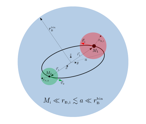
Figure 1: Schematic illustration of the relevant scales involved in the accretion process for a PBH binary system. The Bondi radius of the binary is much bigger than the orbital separation.

In order to study the accretion onto binary PBHs, one has to take into account both global accretion processes (i.e., of the binary as a whole) and local accretion processes (i.e., onto the individual components of the binary). Here we extend the analysis of Ref. [12] to account for generic mass ratios and eccentric orbits. We consider a binary of total mass $M_{\text{\tiny tot}}=M_{1}+M_{2}$, reduced mass $\mu=M_{1}M_{2}/(M_{1}+M_{2})$, mass ratio $q=M_{2}/M_{1}\leq 1$, semi-major axis $a$, and eccentricity $e$. The situation is schematically illustrated in Fig. 1 and described below.

Two distinctive regimes occur depending on how the binary separation compares with the Bondi radius of the binary,

$$r^{\text{\tiny bin}}_{\text{\tiny B}}=\frac{M_{\text{\tiny tot}}}{v^{2}_{\text{\tiny eff}}}\,,$$ (2.10)

where the effective velocity $v_{\text{\tiny eff}}=\sqrt{c_{s}^{2}+v^{2}_{\text{\tiny rel}}}$ depends on the velocity $v_{\text{\tiny rel}}$ of the center of mass of the binary relative to the surrounding gas with mean cosmic density $n_{\text{\tiny gas}}$. Indeed, if $a\gg r^{\text{\tiny bin}}_{\text{\tiny B}}$, accretion occurs onto the two individual PBHs independently (each one moving at a characteristic velocity that also depends on the orbital one), as discussed in the previous section. However, as the binary hardens, the orbital separation becomes much smaller than the Bondi radius of the binary ($a\ll r^{\text{\tiny bin}}_{\text{\tiny B}}$) and, as we shall discuss, this occurs much before GW emission becomes the dominant driving mechanism of the inspiral. In this case, accretion occurs on the binary as a whole at rate given by

$$\dot{M}_{\text{\tiny bin}}=4\pi\lambda m_{H}n_{\text{\tiny gas}}v^{-3}_{\text{\tiny eff}}M^{2}_{\text{\tiny tot}}\,.$$ (2.11)

We now evaluate how the two binary components accrete in this configuration. The PBH positions and velocities with respect to the center of mass are given by [35]

$$r_{1}=\frac{q}{1+q}r,\qquad v_{1}=\frac{q}{1+q}v;\qquad r_{2}=\frac{1}{1+q}r,\qquad v_{2}=\frac{1}{1+q}v$$ (2.12)

in terms of their relative distance and velocity

$$r=a(1-e\,{\rm cos}u),\qquad v=\sqrt{M_{\text{\tiny tot}}\left(\frac{2}{r}-\frac{1}{a}\right)}\,,$$ (2.13)

both expressed as a function of the semi-major axis $a$, eccentricity $e$, and angle $u$. The time evolution of the latter is implicitly given by $\sqrt{a^{3}/M_{\text{\tiny tot}}}(u(t)-e\sin u(t))=t-T$, where $T$ is an integration constant [35]. The PBH effective velocities with respect to the gas are given by

$$v_{\text{\tiny eff,1}}=\sqrt{v^{2}_{\text{\tiny eff}}+v^{2}_{1}},\qquad v_{\text{\tiny eff,2}}=\sqrt{v^{2}_{\text{\tiny eff}}+v^{2}_{2}}.$$ (2.14)

Since the Bondi radius of the binary is much bigger than the typical semi-axis of the binary (see Fig. 1), the total infalling flow of baryons towards the binary is constant, i.e.

$$4\pi m_{H}n_{\text{\tiny gas}}(R)v_{\text{\tiny ff}}(R)R^{2}={\rm const}=\dot{M}_{\text{\tiny bin}}$$ (2.15)

where the free fall velocity of the gas, $v_{\text{\tiny ff}}$, is computed by assuming that at large distances, $R\sim r^{\text{\tiny bin}}_{\text{\tiny B}}$, it reduces to the usual effective velocity $v_{\text{\tiny eff}}$, i.e.

$$v_{\text{\tiny ff}}(R)=\sqrt{v^{2}_{\text{\tiny eff}}+\frac{2M_{\text{\tiny tot}}}{R}-\frac{2M_{\text{\tiny tot}}}{r^{\text{\tiny bin}}_{\text{\tiny B}}}}\,,$$ (2.16)

while $n_{\text{\tiny gas}}(R)$ identifies the density profile at a distance $R$ from the center of mass of the binary,

$$n_{\text{\tiny gas}}(R)=\frac{\dot{M}_{\text{\tiny bin}}}{4\pi m_{H}v_{\text{\tiny ff}}(R)R^{2}}.$$ (2.17)

In other words, being the infalling flow of baryons constant, their density near the binary increases relative to its mean cosmic value at the Bondi radius of the binary.

The accretion rates for the single components of the binary are then given in terms of the effective Bondi radii of the binary components $r_{\text{\tiny B,i}}=M_{i}/v_{\text{\tiny eff,i}}^{2}$ as

$$\dot{M}_{1}=4\pi m_{H}n_{\text{\tiny gas}}(r_{\text{\tiny B,1}})v^{-3}_{\text{\tiny eff,1}}M_{1}^{2},\qquad\dot{M}_{2}=4\pi m_{H}n_{\text{\tiny gas}}(r_{\text{\tiny B,2}})v^{-3}_{\text{\tiny eff,2}}M_{2}^{2}.$$ (2.18)

Note that for the single accretion rates we considered two naked PBHs, for which the parameter $\lambda\approx 1$ at low redshift, while we have described the binary with a dark halo clothing with parameter $\lambda$ which takes into account the ratio of the Bondi radius of the binary with respect to the dark halo radius [9], as discussed above.

Putting together the above formulas, the accretion rates (2.18) can be written in terms of the orbital parameters in a cumbersome (albeit analytical) form,

$$\dot{M}_{1}=\dot{M}_{\text{\tiny bin}}\sqrt{\frac{1+\zeta+(1-\zeta)\gamma^{2}}{2(1+\zeta)(1+q)+(1-\zeta)(1+2q)\gamma^{2}}}\,,$$ (2.19)

$$\dot{M}_{2}=\dot{M}_{\text{\tiny bin}}\sqrt{\frac{(1+\zeta)q+(1-\zeta)q^{3}\gamma^{2}}{2(1+\zeta)(1+q)+(1-\zeta)q^{2}(2+q)\gamma^{2}}}\,,$$ (2.20)

where we defined $\zeta=e\cos u$ and $\gamma^{2}=av^{2}_{\text{\tiny eff}}/\mu q$. The $q\to 0$ limit is particularly simple and does not depend on $e$ nor $u$,

$$\dot{M}_{1}=\dot{M}_{\text{\tiny bin}}+{\cal O}(q)\,,\qquad\dot{M}_{2}=\sqrt{\frac{q}{2}}\dot{M}_{\text{\tiny bin}}+{\cal O}(q^{3/2})\,.$$ (2.21)

In the general case, since the orbital period is much smaller than the accretion time scale $\tau_{\text{\tiny acc}}$, we can average over the angle $u$ and eliminate the explicit time dependence in Eqs. (2.19) and (2.20). After this averaging procedure the dependence on the eccentricity is negligible. Therefore, we can finally write

$$\dot{M}_{1}=\dot{M}_{\text{\tiny bin}}\sqrt{\frac{M_{1}q^{2}+a(1+q)v^{2}_{\text{\tiny eff}}}{(1+q)[2M_{1}q^{2}+a(1+2q)v^{2}_{\text{\tiny eff}}]}}\,,$$

$$\dot{M}_{2}=\dot{M}_{\text{\tiny bin}}\sqrt{\frac{q[M_{1}+a(1+q)v^{2}_{\text{\tiny eff}}]}{(1+q)[2M_{1}+a(2+q)v^{2}_{\text{\tiny eff}}]}}\,.$$ (2.22)

The above rates can be even further simplified when

$$M_{1}q^{2}\gg av^{2}_{\text{\tiny eff}},$$ (2.23)

which is satisfied for $M_{1}\sim\mathcal{O}(M_{\odot})$ and $a\sim{\cal O}(10^{6})M_{1}$ for any $q>10^{-2}$. In this case, the previous expressions reduce to

$$\dot{M}_{1}=\dot{M}_{\text{\tiny bin}}\frac{1}{\sqrt{2(1+q)}},$$

$$\dot{M}_{2}=\dot{M}_{\text{\tiny bin}}\frac{\sqrt{q}}{\sqrt{2(1+q)}}.$$ (2.24)

Note that the expected behaviour $\dot{M}_{1}=\dot{M}_{2}=\dot{M}_{\text{\tiny bin}}/2$ is recovered in the limit $q\to 1$.

As can be checked a posteriori, we will always be interested in a regime in which Eq. (2.24) is an excellent approximation. In the following we shall therefore use these simplified formulas, which have the great advantage to be independent of the orbital parameters. In other words, knowing $\dot{M}_{\text{\tiny bin}}$ and the initial mass ratio, Eq. (2.24) provides the time evolution of the masses of the binary components, regardless of the orbital evolution.

In terms of the Eddington normalised rates, $\dot{m}_{i}=\tau_{\text{\tiny Salp}}\dot{M}_{i}/M_{i}$, one gets

$$\dot{m}_{1}=\dot{m}_{\text{\tiny bin}}\sqrt{\frac{1+q}{2}},\qquad\dot{m}_{2}=\dot{m}_{\text{\tiny bin}}\sqrt{\frac{1+q}{2q}}.$$ (2.25)

The evolution equation for the mass ratio is given by

$$\dot{q}=q\left(\frac{\dot{M}_{2}}{M_{2}}-\frac{\dot{M}_{1}}{M_{1}}\right)=\frac{q}{\tau_{\text{\tiny Salp}}}\left(\dot{m}_{2}-\dot{m}_{1}\right).$$ (2.26)

The above equation shows an important point that will be relevant in the following: if $\dot{m}_{2}>\dot{m}_{1}$, the growth rate of the mass ratio is positive, i.e. the mass ratio grows until it reaches a stationary point when $q=1$ and $\dot{m}_{1}=\dot{m}_{2}$. From Eq. (2.25), it is clear that $\dot{m}_{2}>\dot{m}_{1}$ in any case. This shows that accretion onto a binary PBH implies that the binary masses tend to balance each other on secular time scales.

2.3.3 Effects on the mass function and PBH abundance

In addition to changing the masses and spins of PBHs, accretion also affects their mass distribution function, as well as their mass fraction relative to that of the DM, in a redshift-dependent fashion [11].

Let us define the mass function $\psi(M,z)$ as the fraction of PBHs with mass in the interval $(M,M+{\rm d}M)$ at redshift $z$. For an initial $\psi(M_{\text{\tiny i}},z_{\text{\tiny i}})$ at formation redshift $z_{\text{\tiny i}}$, its evolution is governed by [12, 11]

$$\psi(M(M_{\text{\tiny i}},z),z){\rm d}M=\psi(M_{\text{\tiny i}},z_{\text{\tiny i}}){\rm d}M_{\text{\tiny i}}$$ (2.27)

where $M(M_{\text{\tiny i}},z)$ is the final mass at redshift $z$ for a PBH with mass $M_{\text{\tiny i}}$ at redshift $z_{\text{\tiny i}}$. We stress that – since the evolution of the mass function is needed to re-weight existing constraints on the PBH abundance and since the latter are mainly due to isolated PBHs – for the evolution of the mass function we have considered the evolution of the mass of a single BH; in this case we have to follow Sec. 2.3.1. The main effect of accretion on the mass distribution is to make the latter broader at high masses, producing a high-mass tail that can be orders of magnitude above its corresponding value at formation [11]. A representative example is shown in Fig. 2, where we compare the final mass function (after the accretion phase) with that at formation for some choices of the initial mass distribution.

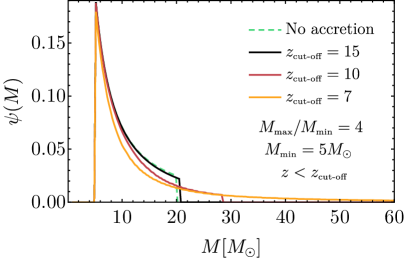
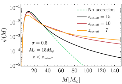
Figure 2: Example of evolution of the power-law (left) and lognormal (right) mass functions.

Finally, also the value of $f_{\text{\tiny\rm PBH}}$ is affected by accretion. Assuming for simplicity a non-relativistic dominant DM component (whose energy density scales as the inverse of the volume), it is easy to show that [11]

$$f_{\text{\tiny\rm PBH}}(z) =\frac{\langle M(z)\rangle}{\langle M(z_{\text{\tiny i}})\rangle(f^{-1}_{\text{\tiny\rm PBH}}(z_{\text{\tiny i}})-1)+\langle M(z)\rangle},$$ (2.28)

where we defined the average mass

$$\langle M(z)\rangle=\int{\rm d}MM\psi(M,z).$$ (2.29)

Due to the presence of accretion, $f_{\text{\tiny\rm PBH}}(z)$ can be significantly larger than $f_{\text{\tiny\rm PBH}}(z_{\text{\tiny i}})$, see an example in Fig. 3.

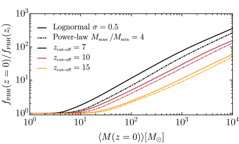
Figure 3: Example of evolution of the PBH abundance for both power-law and lognormal mass functions.

2.3.4 Effects on the PBH spins

The physics of accretion is very complex, since the accretion rate and the geometry of the accretion flow are intertwined, and they are both crucial in determining the evolution of the PBH mass. In addition, the infalling accreting gas onto a PBH can carry angular momentum which crucially determines the geometry of the accreting flow, and the evolution of the PBH spin [12] (see also [36]).

Conditions for a thin-disk formation in isolated and binary PBHs.

For accretion onto an isolated BH, angular momentum transfer is relevant if the typical gas velocity (given by the baryon velocity variance [9]) is larger than the Keplerian velocity close to the PBH. This implies that the minimum PBH mass for which the accreting gas flow is non-spherical is [9, 12]

$$M\mathrel{\hbox to0.0pt{\lower 4.0pt\hbox{\hskip 0.5pt$\sim$}\hss}\raise 1.0pt\hbox{$>$}}6\times 10^{2}M_{\odot}\,D^{1.17}\xi^{4.33}(z)\frac{\left(1+z/1000\right)^{3.35}}{\left[1+0.031\left(1+z/1000\right)^{-1.72}\right]^{0.68}},$$ (2.30)

where $\xi(z)={\rm Max}[1,\langle v_{\text{\tiny eff}}\rangle/c_{s}]$ describes the effect of a (relatively small) PBH proper motion in reducing the Bondi radius, and the constant $D\sim\mathcal{O}(1\div 10)$ takes into account relativistic corrections.

Besides the necessary condition (2.30), the geometry of the disk also depends on the accretion rate. If $\dot{m}<1$ and accretion is non-spherical, an advection-dominated accretion flow (ADAF) may form [41]. When $\dot{m}\gtrsim 1$, the non-spherical accretion can give rise to a geometrically thin accretion disk [42]. For $\dot{m}\gg 1$ the accretion luminosity might be strong enough that the disk “puffs up” and becomes thicker. For simplicity, here we follow Ref. [9] and assume that a thin disk forms when Eq. (2.30) is satisfied and

$$\dot{m}\mathrel{\hbox to0.0pt{\lower 4.0pt\hbox{\hskip 0.5pt$\sim$}\hss}\raise 1.0pt\hbox{$>$}}1\,.$$ (2.31)

In the regimes we are interested in, the latter condition is always more stringent than condition (2.30). Therefore, $\dot{m}\mathrel{\hbox to0.0pt{\lower 4.0pt\hbox{\hskip 0.5pt$\sim$}\hss}\raise 1.0pt\hbox{$>$}}1$ can be considered as the sufficient condition for the formation of a thin disk around an isolated PBH [12].

If instead accretion occurs onto a PBH binary, angular momentum transfer on each PBH is much more efficient [12]. In this case each binary component has a velocity of the order of the orbital velocity $v$. Although the Bondi radius of the individual PBHs is much smaller than the Bondi radius of the binary, it is still parametrically larger than the radius of the innermost stable circular orbit (ISCO, see Eq. (2.34) below). Therefore, the accretion onto the binary components is never spherical and a disk can form. Compared to the aforementioned case of an isolated PBH, in this case condition (2.30) is absent.

To summarize, for both isolated and binary PBHs we can assume that a thin accretion disk forms whenever $\dot{m}\gtrsim 1$ along the cosmic history. Furthermore, since $\dot{m}$ never exceeds unit significantly [12], the thin-disk approximation should be reliable in the super-Eddington regime of PBHs.

Evolution of the spin.

When the conditions for formation of a thin accretion disk are satisfied, i.e. Eq. (2.31), mass accretion is accompanied by an increase of the PBH spin. A thin accretion disk is located along the equatorial plane [42, 43] and therefore the PBH spin is aligned perpendicularly to the disk plane. In such a configuration, one can use a geodesic model to describe the angular-momentum accretion [44].

For circular disk motion the rate of change of the magnitude $J\equiv|\vec{J}|\equiv\chi M^{2}$ of the PBH angular momentum is related to the mass accretion rate (see also Refs. [44, 45, 46, 47])

$$\dot{J}=\frac{L(M,J)}{E(M,J)}\dot{M},$$ (2.32)

where

$$E(M,J)=\sqrt{1-2\frac{M}{3r_{\text{\tiny ISCO}}}}\qquad\text{and}\qquad L(M,J)=\frac{2M}{3\sqrt{3}}\left(1+2\sqrt{3\frac{r_{\text{\tiny ISCO}}}{M}-2}\right)\,,$$ (2.33)

and the ISCO radius reads

$$r_{\text{\tiny ISCO}}(M,J)=M\left[3+Z_{2}-\sqrt{\left(3-Z_{1}\right)\left(3+Z_{1}+2Z_{2}\right)}\right],$$ (2.34)

with $Z_{1}=1+\left(1-\chi^{2}\right)^{1/3}\left[\left(1+\chi\right)^{1/3}+\left(1-\chi\right)^{1/3}\right]$ and $Z_{2}=\sqrt{3\chi^{2}+Z_{1}^{2}}$.

Finally, Eq. (2.32) can be re-arranged to describe the time evolution of the dimensionless Kerr parameter

$$\dot{\chi}=\left({\cal F}(\chi)-2\chi\right)\frac{\dot{M}}{M},$$ (2.35)

where we have defined the combination ${\cal F}(\chi)\equiv L(M,J)/ME(M,J)$, which is only a function of $\chi$. The above spin evolution equation predicts that the spin grows over a typical accretion time scale until it reaches extremality, $\chi=1$. However, radiation effects limit the actual maximum value of the spin to $\chi_{\rm max}=0.998$ [45]. Magnetohydrodynamic simulations of accretion disks around Kerr BHs suggest that the maximum spin might be smaller, $\chi_{\rm max}\simeq 0.9$ [48]. However, this limit may not apply to geometrically thin disks. The geometrically thin-disk approximation is expected to be valid for each PBH when $\dot{m}_{i}\gtrsim 1$. For larger values of the accretion rates, the disk might be geometrically thicker and angular momentum accretion might be less efficient. However, the spin evolution time scale does not change significantly in more realistic accretion models [48].

To summarize, another key prediction of the PBH scenario is the fact that the spin of sufficiently massive PBHs (those that go through epochs of super-Eddington accretion during the cosmic history) should be highly spinning. Note that the condition (2.31) is more easily fulfilled by binary PBHs than by the isolated ones, since in the former case accretion is enhanced by the larger total mass of the binary.

2.4 Summary: theoretical distributions of the PBH binary parameters

In this section we summarize the results for the theoretical distributions of the binary parameters obtained as previously discussed. For ease of notation, we shall denote by $M_{j}$ and $\chi_{j}$ the final mass and spin of the $j$-th binary component; likewise $q$ will be the final mass ratio of the binary. The initial mass and spin of the $j$-th binary component are denoted by $M^{\text{\tiny i}}_{j}$ and $\chi^{\text{\tiny i}}_{j}$ whereas the initial mass ratio is denoted by $q_{\text{\tiny i}}$.  Clearly, in the absence of accretion or hierarchical mergers, the initial and final quantities coincide. In this case the mass and spin distributions are those at formation, see Secs. 2.1 and 2.2.

2.4.1 Mass evolution

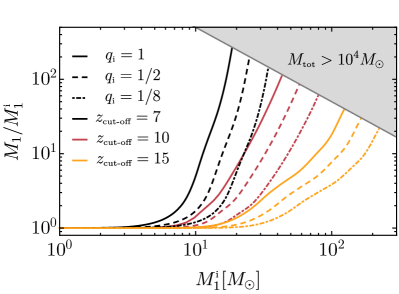
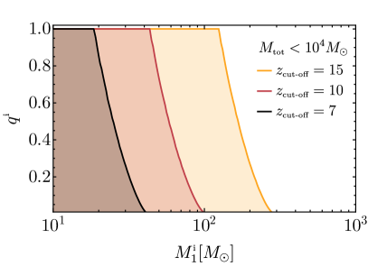
Figure 4: Left: Evolution of the mass of the primary for fixed values of the initial mass ratio. Right: the region in the $(q_{\text{\rm\tiny i}}-M^{\text{\rm\tiny i}}_{1})$ plane (shaded areas) that allows the total final mass of the binary to be below $M_{\text{\rm\tiny tot}}=10^{4}M_{\odot}$. In both panels we considered three different choices of $z_{\text{\rm\tiny cut-off}}$.

As a representative example, in the left panel of Fig. 4 we show the evolution of the primary component mass of the binary for various choices of the initial mass ratio $q_{\text{\tiny i}}$, and for three choices of the cut-off redshift. One can notice that the effect of accretion becomes important above initial masses $\sim 10M_{\odot}$ and is stronger for larger masses and for (initially) nearly-equal mass binaries. Overall, the masses can increase by one or two orders of magnitude due to accretion. Since the merger frequency of binaries with total mass $M_{\text{\tiny tot}}\gtrsim 10^{4}M_{\odot}$ is certainly below the frequency band of current ground-based detectors, we can safely neglect all the binaries that are pushed above that value by accretion. In the right panel of Fig. 4 we show the region in the $q_{\text{\tiny i}}-M^{\text{\tiny i}}_{1}$ plane that allows the total final mass of the binary to be below $M_{\text{\tiny tot}}=10^{4}M_{\odot}$. The parameter space outside the shaded areas would give rise to binaries with $M_{\text{\tiny tot}}>10^{4}M_{\odot}$, which are irrelevant for our study.

Nonetheless, it is intriguing to note that, due to a strong accretion phase at $z\approx(10\div 30)$, PBHs formed with $M^{\text{\tiny i}}\gtrsim 20-100M_{\odot}$, can have much larger masses when they are detected at small redshift. These objects would be natural candidates for intermediate-mass BHs, which are sources for third-generation ground-based detectors and especially for LISA.

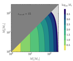
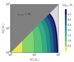
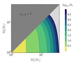
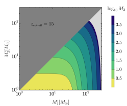
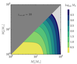
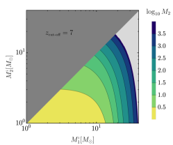
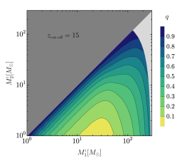
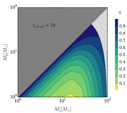
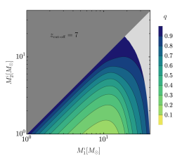
Figure 5: From top to bottom: final masses $M_{1}$, $M_{2}$, and final mass ratio $q$ as a function of the initial masses $(M^{\text{\tiny\rm i}}_{1},M^{\text{\tiny\rm i}}_{2})$. We consider three accretion scenarios parametrised by $z_{\text{\tiny\rm cut-off}}=15$ (left panels), $z_{\text{\tiny\rm cut-off}}=10$ (middle panels), and $z_{\text{\tiny\rm cut-off}}=7$ (right panels).

Since the initial binary parameters are unmeasurable, it is more relevant to analyse the dependence of the final masses $M_{1},M_{2}$ and their mass ratio $q$ in terms of the initial masses $M^{\text{\tiny i}}_{1},M^{\text{\tiny i}}_{2}$. This is done in Fig. 5 for an accretion evolution until the cut-off redshift $z_{\text{\tiny cut-off}}=(15,10,7)$ (from left to right columns).

As shown in Sec. 2.3.2, accretion onto a PBH binary system is such that the secondary body experiences a stronger (specific) accretion rate compared to the primary body. Since the large majority of PBH binaries that merge in the LIGO/Virgo band are formed before accretion is relevant [4], it is expected that strongly-accreting binaries tend to have mass ratios close to unity. This is shown in Fig. 6, in which we present the distribution of the final mass ratio for an initial power-law and lognormal mass function for several choices of ($M_{\text{\tiny min}}$, $M_{\text{\tiny max}}$) and ($\sigma$, $M_{c}$), respectively. The distributions are constructed by drawing the values of ($M^{\text{\tiny i}}_{1},M^{\text{\tiny i}}_{2}$) from a given initial mass function, subject to the constraint that $M_{\text{\tiny tot}}^{\text{\tiny max}}<10^{4}M_{\odot}$. Note, however, that this plot does not represent the distribution of $q$ expected in actual events, since it does not take into account neither how the merger rates depend on the parameters nor the sensitivity curve of LIGO/Virgo, which is optimal for frequencies corresponding to the merger of binary BHs with $M_{\text{\tiny tot}}^{\text{\tiny max}}<10^{2}M_{\odot}$. A direct confrontation with current GW events will be presented in Sec. 5.

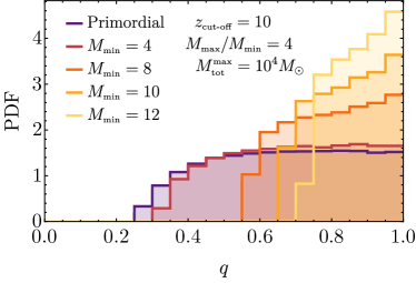
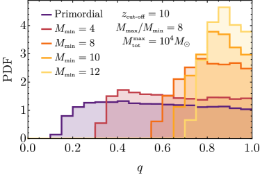
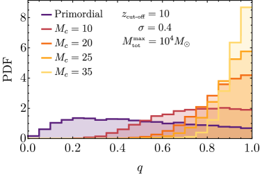
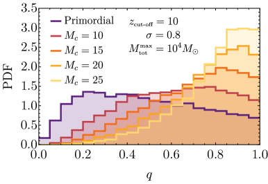
Figure 6: Examples of evolution of the $q$ distribution within the accretion scenario with $z_{\text{\tiny\rm cut-off}}=10$. The distributions are found imposing a cut on the total mass equal to $M_{\text{\tiny\rm tot}}^{\text{\tiny\rm max}}=10^{4}M_{\odot}$. Top and bottom panels correspond to power-law and lognormal mass functions, respectively.

2.4.2 Spin evolution

In the absence of accretion, or if mass accretion is not efficient enough, the spin of PBHs is natal. As discussed in Sec. 2.2 the dimensionless spin parameter $\chi_{\text{\tiny i}}$ in the most likely formation scenarios is of the order of the percent or smaller, although larger values are predicted in less standard scenarios, see e.g. [27, 28].

The situation changes drastically in the case of efficient accretion. In Fig. 7 we show the final spins of the PBH binary components as a function of their final masses for three different choices of $z_{\text{\tiny cut-off}}$. Besides the quantitative difference between different choices of $z_{\text{\tiny cut-off}}$, the qualitative trend is the same. Namely, the final mass and final spin of the PBHs are correlated: low-mass PBHs are slowly spinning or non-spinning, whereas high-mass PBHs are rapidly spinning. The mass scale at which this continuous transition occurs depends on the cut-off redshift and it is always around $(10\div 40)\,M_{\odot}$. In particular, smaller cut-offs favour a lower-mass transition, as expected by the fact that in this case the accreting phase lasts longer during the cosmic evolution.

In Fig. 8 we show the distribution of the effective spin parameter defined as

$$\chi_{\text{\tiny eff}}=\frac{\vec{J}_{1}/M_{1}+\vec{J}_{2}/M_{2}}{M_{1}+M_{2}}\cdot\hat{L},$$ (2.36)

where $M_{1}$ and $M_{2}$ are the individual BH masses, $\vec{J}_{1}$ and $\vec{J}_{2}$ are the corresponding angular-momentum vectors, and $\hat{L}$ is the direction of the orbital angular momentum. Following Ref. [12] we have averaged over the angles between the total angular momentum and the individual PBH spins. We have plotted $\chi_{\text{\tiny eff}}$ as a function of the final PBH mass $M_{1}$ for different fixed values of the mass ratio parameter $q$. When accretion is present, such distributions reflect the transition from initially vanishing values of $\chi_{\text{\tiny eff}}$ to large ones. In the top two rows of Fig. 8 (for $q=1$ and $q=1/2$), we have shown only the current data which are compatible (within their reported errors) with the corresponding chosen value of $q$. In the third row ($q=1/4$) we report only GW190412 as a reference.

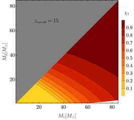
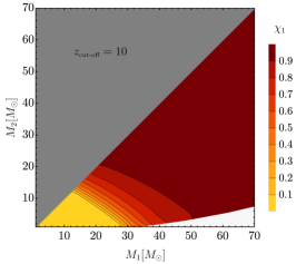
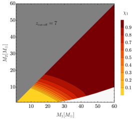
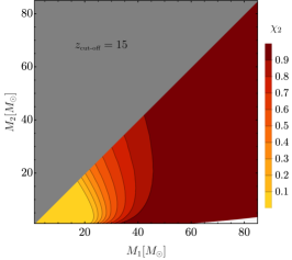
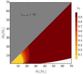
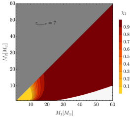
Figure 7: Final spins $\chi_{1}$ (top panels) and $\chi_{2}$ (bottom panels) as functions of the final masses $(M_{1},M_{2})$. As in Fig. 5, from left to right we consider three cut-off redshifts below which accretion is suppressed.

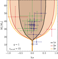
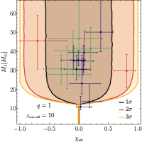
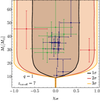
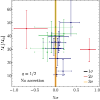
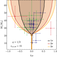
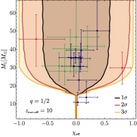
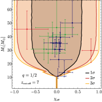
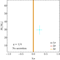
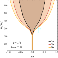
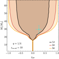
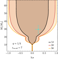
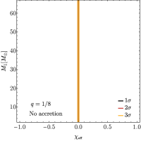
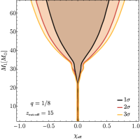
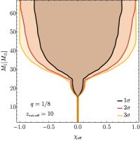
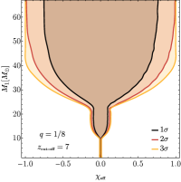
Figure 8: The distribution of $\chi_{\text{\tiny\rm eff}}$ as a function of the PBH mass $M_{1}$ for selected values of the parameter $q$. Blue data points refer to the events listed in Ref. [1], whereas green and red data points refer to the events discovered in Refs. [49, 50]; the red data points refer to GW151216 and GW170403, for which the measured value of $\chi_{\text{\tiny\rm eff}}$ is significantly affected by the prior on the spin angles [51]. The cyan data point refers to GW190412 recently reported in Ref. [2].

2.5 Limitations of the accretion model

Accretion onto compact objects through the cosmic history is a complex phenomenon and the accretion rate relies on a set of assumptions, above all through the dependence on the velocity. While from the discussion of the previous sections it seems clear that accretion should play a relevant role, it is also important to spell out the main uncertainties in the accretion modelling [9, 8, 52].

• Local feedback: our analysis neglects the effect of feedback on the accretion flow. The effect of local heating for the PBH masses of interest for LIGO/Virgo can be safely neglected [8, 52].

• Global feedback & X-ray pre-heating: this effect was estimated in [8], including the X-ray heating of the gas and the extra contribution due to PBH accretion, but neglecting other possible sources of X-ray heating [53]. However, since then, the analysis of the cosmic ionisation provided in Ref. [8] has been strongly revisited by later work, in particular after GW150914 and the suggestion that those BHs might be of primordial origin [5]. Indeed, the detailed analysis of Ref. [52] shows that global feedback is much less important for LIGO/Virgo BHs. In particular, taking all relevant effects into account, Ref. [52] found an accretion rate which is consistent with that estimated by Ref. [8] without the effect of global heating. Modelling the temperature of the intergalactic medium at redshift $10\lesssim z\lesssim 30$ is particularly relevant, since an increase in the temperature is followed by an increase in the sound speed and, in turn, by a reduction of the accretion rate.

• DM halo: the accretion rate computed in our model is consistent with that of Ref. [52], with the important inclusion of a DM halo, which seems inevitable if PBHs form a small fraction of the DM, at least if the latter is of particle origin.

• Structure formation: part of the population of PBHs starts falling in the gravitational potential well of large-scale structures after redshift around $z\simeq 10$, experiencing an increase of the relative velocity up to one order of magnitude, see for example Ref. [54] for a recent analysis. This will result in a consequent suppression of the accretion rate [9, 56, 55]. While this motivates our choice $z_{\text{\tiny cut-off}}=10$, the precise dynamics depends on the complex modelling of the global thermal feedback and the change in the relative velocity due to the structure formation. Furthermore, it is hard to estimate the fraction of PBHs that stop accreting efficiently enough due to this effect. For example, the captured PBHs might settle at the center of the halo within a Hubble time, due e.g. to dynamical friction effects, and might keep accreting efficiently.

• Spherical accretion & disk geometry: most of the semi-analytical studies on accretion onto compact objects necessarily assume a quasi-spherical flow. However, this approximation might break down, e.g. in the case of outflows [57]. The efficiency of the latter in reducing the accretion rate depends on the geometry of the accretion flow and on the relative direction of the outflow.

• Angular momentum transfer: As discussed above, when $\dot{m}\sim 1$ the disk is geometrically thin and can be described with a geodesic model. When $\dot{m}\ll 1$ or $\dot{m}\gg 1$, the geometry of the disk is different, and this impacts on the accretion luminosity and feedback. In the super-Eddington regime the disk is expected to “puff up”, becoming geometrically thicker. Angular momentum accretion in this case is more complex, although numerical simulations suggest that the spin evolution time scale does not change significantly [48].

While the above details require complex and model-dependent simulations, the uncertainties in certain aspects of the accretion model can be parametrised in an agnostic way through a cut-off redshift $z_{\text{\tiny cut-off}}$. For instance, as far as the X-ray pre-heating effect [53] on the accretion rate is concerned, the suppression factor in $\dot{m}$ with respect to the case of no X-ray pre-heating may be at most an order of magnitude or smaller. Most importantly, this effect can be caught in our model by increasing the value of $z_{\text{\tiny cut-off}}$ without including the X-ray pre-heating.

Based on the above discussion, we consider $z_{\text{\tiny cut-off}}=10$ as the most reasonable choice for the cut-off redshift; the value $z_{\text{\tiny cut-off}}=7$ advocated in Ref. [9] might be considered as an optimistic choice that assumes a non-negligible fraction of PBHs which keeps accreting significantly even after structure formation, whereas larger values of the cut-off, e.g. $z_{\text{\tiny cut-off}}=15$ would suppress the effect of accretion and correspond to a scenario in which the temperature of the intergalactic medium is high enough even before reionisation.

3 Binary evolution

Having discussed the masses and spins of isolated and binaries PBHs, we now turn our attention to the evolution of PBH binaries. First we consider the case in which accretion is absent or inefficient, in which case the binary evolves only through GW radiation-reaction, which we review following Sec. 4.1 of Ref. [60]. Then, we consider the case in which baryonic mass accretion is modelled as discussed in the previous sections, extending the results of Ref. [61] to the case of accretion-driven inspiral for eccentric binaries with generic mass ratio.

3.1 GW-driven evolution

In the absence of GW radiation-reaction, the eccentricity $e$ and semi-major axis $a$ are constants of motion and can be expressed in terms of the angular momentum and energy as

$$e^{2}=1+\frac{2EL^{2}}{M_{\text{\tiny tot}}^{2}\mu^{3}}\,,\qquad a=\frac{GM_{\text{\tiny tot}}\mu}{2|E|}\,.$$ (3.1)

To the leading order in the weak-field/slow-motion approximation, one can use the quadrupole formula to evaluate the energy and angular momentum losses through the GW emission. The energy and angular momentum of the binary evolves as [62, 63]

$$\frac{{\rm d}E}{{\rm d}t} =-\frac{32}{5}\frac{\mu^{2}M_{\text{\tiny tot}}^{3}}{a^{5}}\frac{1}{(1-e^{2})^{7/2}}\left(1+\frac{73}{24}e^{2}+\frac{37}{96}e^{4}\right),$$

$$\frac{{\rm d}L}{{\rm d}t} =-\frac{32}{5}\frac{\mu^{2}M_{\text{\tiny tot}}^{5/2}}{a^{7/2}}\frac{1}{(1-e^{2})^{2}}\left(1+\frac{7}{8}e^{2}\right).$$ (3.2)

In terms of the adiabatic evolution of $e$ and $a$, one can recast the system of equations in the form

$$\frac{{\rm d}a}{{\rm d}t} =-\frac{64}{5}\frac{\mu M_{\text{\tiny tot}}^{2}}{a^{3}}\frac{1}{(1-e^{2})^{7/2}}\left(1+\frac{73}{24}e^{2}+\frac{37}{96}e^{4}\right),$$

$$\frac{{\rm d}e}{{\rm d}t} =-\frac{304}{15}\frac{\mu M_{\text{\tiny tot}}^{2}}{a^{4}}\frac{e}{(1-e^{2})^{5/2}}\left(1+\frac{121}{304}e^{2}\right).$$ (3.3)

This system can be solved to find an estimate for the merging time $t_{c}$, here defined as $a(t_{c})=0$. For an initial orbit with $e(t_{\text{\tiny i}})=e_{\text{\tiny i}}$ and $a(t_{\text{\tiny i}})=a_{\text{\tiny i}}$ one finds

$$t_{c}(a_{\text{\tiny i}},e_{\text{\tiny i}})=t_{c}(a_{\text{\tiny i}})\frac{48}{19}\frac{1}{g^{4}(e_{\text{\tiny i}})}\int_{0}^{e_{\text{\tiny i}}}{\rm d}e\frac{g^{4}(e)(1-e^{2})^{5/2}}{e(1+121e^{2}/304)}\,,$$ (3.4)

where we defined the function

$$g(e)=\frac{e^{12/19}}{1-e^{2}}\left(1+\frac{121}{304}e^{2}\right)^{870/2299}\,.$$ (3.5)

For a circular orbit, Eq. (3.4) reduces to

$$t_{c}(a_{\text{\tiny i}},e_{\text{\tiny i}}=0)\equiv t_{c}(a_{\text{\tiny i}})=\frac{5}{256}\frac{a_{\text{\tiny i}}^{4}}{M_{\text{\tiny tot}}^{2}\mu}.$$ (3.6)

Conversely, in the limit $e_{\text{\tiny i}}\to 1$, one finds that

$$t_{c}(a_{\text{\tiny i}},e_{\text{\tiny i}}\to 1)\simeq t_{c}(a_{\text{\tiny i}})\frac{768}{429}(1-e_{\text{\tiny i}}^{2})^{7/2}.$$ (3.7)

The parameters leading to a coalescence time equal to the age of the universe, $t_{0}=13.7\,{\rm Gyr}$, are shown in Fig. 9. As one can notice, the initial value of $a_{\text{\tiny i}}$ diverges as $e_{\text{\tiny i}}$ tends towards unity, since the coalescence time tends to shrink rapidly in that limit.

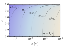
Figure 9: The contour lines indicate the combination of the parameters $e_{\text{\tiny\rm i}}$ and $a_{\text{\tiny\rm i}}$ giving a coalescence time equal to the age of the universe $t_{c}(a_{\text{\tiny\rm i}},e_{\text{\tiny\rm i}})=t_{0}$. The label indicates $M_{1}$ and the mass ratio considered is $q=1$, $1/2$ and $1/8$ respectively.

The above relation is used by [6, 4] to compute an estimate of the merger rate, as we discuss in Sec. 4.

3.2 Accretion-driven evolution

Accretion introduces a further secular change to the orbital parameters, in addition to GW radiation-reaction [64, 65, 61]. As we are going to discuss, due to the time scales involved in the problem, we can study the accretion-driven phase and the GW-driven phase separately. Indeed, since for $z<z_{\text{\tiny cut-off}}$ accretion is drastically suppressed, the evolution of the binary from $z_{\text{\tiny cut-off}}$ to the redshift of detection (which we shall assume to be $z\approx 0$ having in mind the current horizons of LIGO and Virgo) is governed by GW emission only. From Eq. (3.4), a merger occurring at $z\approx 0$ corresponds to a binary with orbital separation $a={\cal O}(10^{11}\,{\rm m})$ at $z_{\text{\tiny cut-off}}=10$. In this configuration the time scale of variation of the semi-major axis due to GW emission is

$$T_{\text{\tiny GW}} \sim\left.\frac{a}{\dot{a}}\right|_{\text{\tiny GW}}=4\times 10^{17}\left(\frac{a}{1.4\times 10^{11}{\rm m}}\right)^{4}\left(\frac{M}{30M_{\odot}}\right)^{-3}\left(\frac{1-e^{2}}{0.1}\right)^{7/2}\,{\rm s}$$ (3.8)

where the normalisation $a=1.4\times 10^{11}{\rm m}$ has been chosen as the one giving a merger in a time equal to the age of the universe for binary components of equal mass $M=30M_{\odot}$ and $e=0.95$. As can be directly checked, owing to the strong dependence $T_{\text{\tiny GW}}\propto a^{4}$, for $z>z_{\text{\tiny cut-off}}$ the typical accretion time scale (2.9) is much smaller than the one governing GW radiation-reaction. In other words, we can assume that the inspiral is driven solely by accretion when $z>z_{\text{\tiny cut-off}}$ and solely by GW radiation-reaction when $z<z_{\text{\tiny cut-off}}$.

It is also worth noting that, for the range of parameters we are interested in, the mass accretion time scale (2.9) is always much larger than the characteristic orbital time scale,

$$T_{\text{\tiny orbital}}\sim\left(\frac{M_{\text{\tiny tot}}}{a^{3}}\right)^{-1/2}\sim 8\times 10^{5}\left(\frac{M}{30M_{\odot}}\right)^{-1/2}\left(\frac{a}{1.4\cdot 10^{11}\,{\rm m}}\right)^{3/2}\,{\rm s}\,.$$ (3.9)

Therefore one can treat the mass accretion as an adiabatic process keeping constant the adiabatic invariants of the elliptical motion, as we now discuss.

If the masses vary adiabatically, one can compute the action variables $I_{k}=\int p{\rm d}k/(2\pi)$ for the elliptic motion (where $k=r,\phi$ are the polar coordinates) and then employ the fact that they are adiabatic invariants. Specifically, the adiabatic invariants for the Keplerian two-body problem are [66]

$$I_{\phi} =\frac{1}{2\pi}\int_{0}^{2\pi}p_{\phi}{\rm d}\phi=L_{z},$$ (3.10)

$$I_{r} =\frac{1}{2\pi}\int_{r_{\rm min}}^{r_{\rm max}}p_{r}{\rm d}r=-L_{z}+\sqrt{M_{\text{\tiny tot}}\mu^{2}a},$$ (3.11)

where we recall the definition of energy and angular momentum of the binary

$$E =-\frac{\mu M_{\text{\tiny tot}}}{2a},\qquad L_{z}=\sqrt{\frac{M_{\text{\tiny tot}}^{2}\mu^{3}(e^{2}-1)}{2E}}=\sqrt{1-e^{2}}\sqrt{M_{\text{\tiny tot}}\mu^{2}a}.$$ (3.12)

The invariance of $I_{\phi}$ and $I_{r}$ implies that

$$\frac{{\rm d}I_{\phi}}{{\rm d}t} =\frac{\partial L_{z}}{\partial e}\frac{\partial e}{\partial t}+\frac{\partial L_{z}}{\partial a}\frac{\partial a}{\partial t}+\frac{\partial L_{z}}{\partial\mu}\frac{\partial\mu}{\partial t}+\frac{\partial L_{z}}{\partial M_{\text{\tiny tot}}}\frac{\partial M_{\text{\tiny tot}}}{\partial t}=0\,,$$

$$\frac{{\rm d}I_{r}}{{\rm d}t} =\frac{\partial I_{r}}{\partial e}\frac{\partial e}{\partial t}+\frac{\partial I_{r}}{\partial a}\frac{\partial a}{\partial t}+\frac{\partial I_{r}}{\partial\mu}\frac{\partial\mu}{\partial t}+\frac{\partial I_{r}}{\partial M_{\text{\tiny tot}}}\frac{\partial M_{\text{\tiny tot}}}{\partial t}=0.$$ (3.13)

It is easy to prove that the system of equations can be recast as

$$\frac{\partial a}{\partial t} =-\frac{2a}{\mu}\frac{\partial\mu}{\partial t}-\frac{a}{M_{\text{\tiny tot}}}\frac{\partial M_{\text{\tiny tot}}}{\partial t},$$

$$\frac{\partial e}{\partial t} =0\,,$$ (3.14)

which shows that the eccentricity is a constant of motion for an accretion-driven inspiral. This does not come as a surprise as the eccentricity can be expressed in terms of the adiabatic invariants as [66]

$$e=\sqrt{1-\left(\frac{I_{\phi}}{I_{\phi}+I_{r}}\right)^{2}}.$$ (3.15)

The only non-trivial dynamical equation can be written as

$$\frac{\dot{a}}{a}+2\frac{\dot{\mu}}{\mu}+\frac{\dot{M}_{\text{\tiny tot}}}{M_{\text{\tiny tot}}}=0.$$ (3.16)

This results recovers the one found in Ref. [61] in the absence of GW emission and for circular binaries, and extends it for a generic eccentricity, which remains a constant of motion.

Finally, it is convenient to write Eq. (3.16) in terms of the mass accretion rates of the isolated objects

$$\frac{\dot{a}}{a}+\frac{M_{2}(M_{1}+2M_{2})\dot{M}_{1}+M_{1}(2M_{1}+M_{2})\dot{M}_{2}}{M_{1}M_{2}(M_{1}+M_{2})}=0\,.$$ (3.17)

In general, this equation is coupled to the evolution equations for $M_{1}$ and $M_{2}$, namely Eqs. (2.22). However, within the aforementioned approximations, one can evolve $M_{i}$ using Eq. (2.24) and finally evolve the semi-axis major using Eq. (3.17). In the limit $q\to 1$, i.e. $M_{1}=M_{2}$, Eq. (3.17) simplifies to the more familiar form

$$\frac{\dot{a}}{a}+3\frac{\dot{M}_{1}}{M_{1}}=0\,.$$ (3.18)

4 PBH merger rates and phenomenology

After the discussion about the evolution of the PBH binary, we move to the computation of the PBH merger rate both without and including accretion, and we will then discuss its impact on the PBH phenomenology.

4.1 Merger rates without accretion

Following the notation of Ref. [73], one can write down the differential merger rate at the time of coalescence $t$ in the form

$${\rm d}R=\frac{1.6\times 10^{6}}{{\rm Gpc^{3}\,yr}}f_{\text{\tiny\rm PBH}}^{\frac{53}{37}}(z_{\text{\tiny i}})\left(\frac{t}{t_{0}}\right)^{-\frac{34}{37}}\eta_{\text{\tiny i}}^{-\frac{34}{37}}\left(\frac{M^{\text{\tiny i}}_{\text{\tiny tot}}}{M_{\odot}}\right)^{-\frac{32}{37}}S\left(M^{\text{\tiny i}}_{\text{\tiny tot}},f_{\text{\tiny\rm PBH}}(z_{\text{\tiny i}})\right)\psi(M^{\text{\tiny i}}_{1},z_{\text{\tiny i}})\psi(M^{\text{\tiny i}}_{2},z_{\text{\tiny i}}){\rm d}M^{\text{\tiny i}}_{1}{\rm d}M^{\text{\tiny i}}_{2},$$ (4.1)

where $f_{\text{\tiny\rm PBH}}(z_{\text{\tiny i}})$ is the initial fraction of DM in the form of PBHs, $\eta_{\text{\tiny i}}=\mu^{\text{\tiny i}}/M^{\text{\tiny i}}_{\text{\tiny tot}}$ is the symmetric mass ratio, defined in terms of the reduced mass $\mu^{\text{\tiny i}}=M^{\text{\tiny i}}_{1}M^{\text{\tiny i}}_{2}/M^{\text{\tiny i}}_{\text{\tiny tot}}$ and total mass $M^{\text{\tiny i}}_{\text{\tiny tot}}=M^{\text{\tiny i}}_{1}+M^{\text{\tiny i}}_{2}$ of the binary components at the formation time, and $\psi(M^{\text{\tiny i}},z_{\text{\tiny i}})$ identifies the PBH mass function at the formation time $z_{\text{\tiny i}}$, normalised to unity.

The suppression factor $S$ is introduced in order to keep into account the effect of the matter density perturbations and possible modifications due to the size of the empty region around the binary. Its expression is given by [73]

$$S\left(M^{\text{\tiny i}}_{\text{\tiny tot}},f_{\text{\tiny\rm PBH}}(z_{\text{\tiny i}})\right)=\frac{e^{-\bar{N}(y)}}{\Gamma(21/37)}\int{\rm d}vv^{-\frac{16}{37}}{\rm exp}\left[-\bar{N}(y)\left\langle m\right\rangle\int\frac{{\rm d}m}{m}\psi(m,z_{\text{\tiny i}})F\left(\frac{m}{\left\langle m\right\rangle}\frac{v}{\bar{N}(y)}\right)-\frac{3\sigma_{M}^{2}v^{2}}{10f_{\text{\tiny\rm PBH}}^{2}(z_{\text{\tiny i}})}\right]$$ (4.2)

in terms of the generalised hypergeometric function

$$F(z)=\tensor[_{1}]{F}{{}_{2}}\left(-\frac{1}{2};\frac{3}{4};\frac{5}{4};-\frac{9z^{2}}{16}\right)-1\,,$$ (4.3)

the rescaled variance of matter density perturbations $\sigma_{M}^{2}=(\Omega_{M}/\Omega_{\rm DM})^{2}\left\langle\delta_{M}^{2}\right\rangle\simeq 3.6\cdot 10^{-5}$ at the time at which the binary is formed, and

$$\left\langle m\right\rangle=\left(\int\frac{1}{m}\psi(m,z_{\text{\tiny i}}){\rm d}m\right)^{-1}.$$ (4.4)

The number $\bar{N}(y)$ of PBHs in a spherical volume of radius $y$ is chosen such that the binaries do not get destroyed by other PBHs, i.e.

$$\bar{N}(y)=\frac{M^{\text{\tiny i}}_{\text{\tiny tot}}}{\left\langle m\right\rangle}\frac{f_{\text{\tiny\rm PBH}}(z_{\text{\tiny i}})}{f_{\text{\tiny\rm PBH}}(z_{\text{\tiny i}})+\sigma_{M}}.$$ (4.5)

The integral over the masses in the suppression factor gives an estimate of the typical mass of the perturber PBHs responsible for the torque, which prevents two PBHs to collide directly and is responsible for forming the binary itself.

In Fig. 10 we show the behaviour of the suppression factor for the cases of a lognormal and power-law mass function.

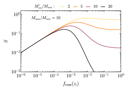
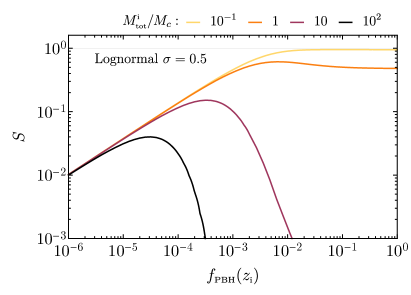
Figure 10: Left: Suppression factor for a power-law mass function with $M_{\text{\tiny\rm max}}=10M_{\text{\tiny\rm min}}$ and various $M^{\text{\tiny i}}_{\text{\tiny\rm tot}}$. Right: Suppression factor for a lognormal mass function with $\sigma=0.5$.

4.2 Merger rates with accretion

In this subsection we will describe the main impact of accretion on the PBH merger rate.

As already discussed in Sec. 3, due to the time scales involved in the problem, one can study the accretion-driven and the GW-driven binary evolution separately. Indeed, accretion dominates the evolution of the binary up to redshift $z_{\text{\tiny cut-off}}$, while GW radiation-reaction is dominant from that redshift up to the detection time.

To understand the effect of accretion on the merger rate we remind that, using the formalism of Ref. [73], the latter is defined by integrating the probability distribution of the orbital parameters

$${\rm d}R(t)=\int{\rm d}a{\rm d}e\frac{{\rm d}P}{{\rm d}e}\delta\left(t-t_{c}(\mu,M_{\text{\tiny tot}},a,e)\right)$$ (4.6)

at the coalescence time of the binary, which has been computed in Sec. 3 without accretion and which we report here for convenience in a more compact form

$$t_{c}=\frac{3}{85}\frac{a_{\text{\tiny i}}^{4}{(1-e_{\text{\tiny i}}^{2})}^{7/2}}{\eta(z_{\text{\tiny i}})M_{\text{\tiny tot}}^{3}(z_{\text{\tiny i}})},$$ (4.7)

where all the quantities are set at the formation time $z_{\text{\tiny i}}$.

In the presence of accretion the masses change in time. Even though the ellipticity is a constant of motion, the semi-major axis $a$ does evolve with time due to the masses evolution, as one can see from Eq. (3.16). This will have an impact on the coalescence time of the binary. Since the accretion-driven phase occurs earlier and independently of GW emission, once accretion is included the coalescence time becomes

$$t^{\text{\tiny acc}}_{c}=\frac{3}{85}\frac{{\cal N}^{4}a_{\text{\tiny i}}^{4}{(1-e_{\text{\tiny i}}^{2})}^{7/2}}{\eta(z_{\text{\tiny cut-off}})M_{\text{\tiny tot}}^{3}(z_{\text{\tiny cut-off}})}\equiv\frac{{\cal N}^{4}}{\mathcal{S}}t_{c}(M^{\text{\tiny i}}_{j}),$$ (4.8)

where we have defined the factor

$${\cal S}=\frac{\eta(z_{\text{\tiny cut-off}})M_{\text{\tiny tot}}^{3}(z_{\text{\tiny cut-off}})}{\eta(z_{\text{\tiny i}})M_{\text{\tiny tot}}^{3}(z_{\text{\tiny i}})}$$ (4.9)

which keeps into account the masses evolution from initial time $z_{\text{\tiny i}}$ to the cut-off redshift $z_{\text{\tiny cut-off}}$, and the shrinking factor of the orbit

$${\cal N}\equiv\frac{a(z_{\text{\tiny cut-off}})}{a_{\text{\tiny i}}}=\exp\left[-\int_{t_{\text{\tiny i}}}^{t_{\text{\tiny cut-off}}}{\rm d}t\left(\frac{\dot{M}_{\text{\tiny tot}}}{M_{\text{\tiny tot}}}+2\frac{\dot{\mu}}{\mu}\right)\right],$$ (4.10)

which properly considers the semi-major axis evolution. As we discussed, for $z<z_{\text{\tiny cut-off}}$ accretion is negligible, so the binary proceeds in the standard GW radiation-reaction scenario, but with different masses with respect to the no accretion case.

Implementing the fact that the suppression factor does not depend on time and using Eq. (2.27) for the mass function evolution, one can rescale the coalescence time to compute the final differential merger rate as

$${\rm d}R_{\text{\tiny acc}}(t,M_{j},f_{\text{\tiny\rm PBH}}(z_{\text{\tiny i}})) =\frac{\mathcal{S}}{{\cal N}^{4}}{\rm d}R\left(t\mathcal{S}/{\cal N}^{4},M^{\text{\tiny i}}_{j},f_{\text{\tiny\rm PBH}}(z_{\text{\tiny i}})\right)$$

$$=\mathcal{N}^{-12/37}\mathcal{S}^{3/37}{\rm d}R\left(t,M^{\text{\tiny i}}_{j},f_{\text{\tiny\rm PBH}}(z_{\text{\tiny i}})\right)$$ (4.11)

where with $M^{\text{\tiny i}}_{j}$ and $M_{j}$ we identify respectively the couple $(M_{1},M_{2})$ at the formation and final time. In the last line the merger rate in terms of the initial quantities is explicitly given by Eq. (4.1). As such, the bounds coming from merger rates do not depend upon the evolution of the mass functions discussed in subsection 2.3.3.

4.3 Phenomenology of PBH mergers without accretion

In this subsection we will discuss the implications of the physics of the PBH mergers on their phenomenology, by focusing on the constraints on the PBH abundance both from the total number of observed binary BH merger events by the LIGO/Virgo collaboration, and from the absence of the stochastic GW background produced by unresolved sources. We will follow the procedure outlined in Ref. [73], without including the effects of accretion. The latter will be discussed in Sec. 4.4.

4.3.1 Likelihood analysis for GW observations without accretion

One can start by performing a maximum-likelihood analysis, considering all the BH merger events observed by the LIGO/Virgo collaboration to date [1, 2] and assuming that they all have a primordial origin, to find out the best-fit values for the parameters of the PBH mass function. For concreteness, we shall assume either a lognormal or a power-law distribution.

The log-likelihood function is given by

$${\cal L}=\sum_{j}{\rm ln}\frac{\int{\rm d}R(M_{1},M_{2},z)/(1+z){\rm d}V_{c}(z)p_{j}(M_{j,1}|M_{1})p_{j}(M_{j,2}|M_{2})p_{j}(z_{j}|z)\Theta(\rho(M_{1},M_{2},z)-\rho_{c})}{\int{\rm d}R(M_{1},M_{2},z)/(1+z){\rm d}V_{c}(z)\Theta(\rho(M_{1},M_{2},z)-\rho_{c})}\,,$$ (4.12)

where the experimental uncertainties of the detected events are assumed to be described by Gaussian probabilities $p_{j}(M_{j}|M)$ to observe a BH mass $M_{j}$ given that the BH has mass $M$, and by Gaussian probabilities $p_{j}(z_{j}|z)$ to observe a merger at redshift $z_{j}$ given that it happens at redshift $z$.

The integral is performed over the masses and redshift, in terms of the PBH merger rate ${\rm d}R(M_{1},M_{2},z)$ shown in Eq. (4.1), and of the comoving volume per unit redshift

$$\frac{{\rm d}V_{c}(z)}{{\rm d}z}=\frac{4\pi}{H_{0}}\frac{D_{c}^{2}(z)}{E(z)}=\frac{4\pi}{H_{0}^{2}}\frac{1}{E(z)}\left(\int_{0}^{z}\frac{{\rm d}z^{\prime}}{E(z^{\prime})}\right)^{2},$$ (4.13)

where the comoving distance $D_{c}$ is

$$D_{c}(z)=\frac{1}{H_{0}}\int_{0}^{z}\frac{{\rm d}z^{\prime}}{E(z^{\prime})}$$ (4.14)

with

$$E(z^{\prime})=\sqrt{\Omega_{r}(1+z^{\prime})^{4}+\Omega_{m}(1+z^{\prime})^{3}+\Omega_{\text{\tiny K}}(1+z^{\prime})^{2}+\Omega_{\Lambda}},$$ (4.15)

and $\Omega_{\text{\tiny K}}=0.0007$, $\Omega_{r}=5.38\times 10^{-5}$, $\Omega_{\Lambda}=0.685$, $\Omega_{m}=0.315$, $h=0.674$, $H_{0}=1.0227\times 10^{-10}h\,{\rm yr}^{-1}$. The additional factor of redshift $1/(1+z)$ is introduced to account for the difference in the clock rates at the time of merger and detection. The Heaviside function $\Theta$ is introduced in Eq. (4.12) to implement a detectability threshold based on the signal-to-noise ratio (SNR) of the GW events, $\rho_{c}=8$. The optimal signal-to-noise ratio $\rho_{\text{\tiny opt}}$ of individual GW events for a source with masses $M_{1},M_{2}$ at a redshift $z$ is given by [74]

$$\rho_{\text{\tiny opt}}^{2}(M_{1},M_{2},z)\equiv\int_{0}^{\infty}\frac{4|\widetilde{h}(\nu)|^{2}}{S_{n}(\nu)}{\rm d}\nu$$ (4.16)

where the strain noise for the O2 run has been taken from Ref. [75] and its analytical fit in the frequency range $\nu\in[10,5000]\,{\rm Hz}$ is given by

$$S_{n,{\rm O2}}^{1/2}(\nu)=\exp\left[\sum_{i=0}^{6}c_{i}\log^{i}(\nu)\right],$$ (4.17)

with

$$c_{0} =33.3329,\quad c_{1}=-75.7393,\quad c_{2}=27.1742,\quad c_{3}=-5.10534,$$

$$c_{4} =0.524229,\quad c_{5}=-0.0273956,\quad c_{6}=0.000557901.$$ (4.18)

The GW strain signal $\widetilde{h}$ is given in Fourier space by [74]

$$\widetilde{h}(\nu)=\sqrt{\frac{5}{8}}\frac{1}{D_{\text{\tiny L}}\pi}\frac{1}{\nu}\left(\frac{{\rm d}E_{\text{\tiny GW}}(\nu)}{{\rm d}\nu}\right)^{1/2}e^{i\phi(\nu)}$$ (4.19)

where $\phi(\nu)$ is the phase of the waveform, not relevant for the SNR, and $D_{\text{\tiny L}}$ identifies the luminosity distance from the source in terms of the comoving distance $D_{c}$ as

$$D_{\text{\tiny L}}(z)=(1+z)D_{c}(z)=(1+z)\frac{1}{H_{0}}\int_{0}^{z}\frac{{\rm d}z^{\prime}}{E(z^{\prime})}.$$ (4.20)

For the GW energy spectrum ${\rm d}E_{\text{\tiny GW}}$ with frequency between $(\nu,\nu+{\rm d}\nu)$ we use a phenomenological expression which, in the non-spinning limit, is given by [74, 76]

$$\frac{{\rm d}E_{\text{\tiny GW}}(\nu)}{{\rm d}\nu}=\frac{\pi^{2/3}}{3}M_{\text{\tiny tot}}^{5/3}\eta\times\left\{\begin{array}[]{rl}&\nu^{-1/3}\quad\text{for}\quad\nu<\nu_{1},\\ &\frac{\nu}{\nu_{1}}\nu^{-1/3}\quad\text{for}\quad\nu_{1}\leq\nu<\nu_{2},\\ &\frac{\nu^{2}}{\nu_{1}\nu_{2}^{4/3}}\frac{\sigma^{4}}{(4(\nu-\nu_{2})^{2}+\sigma^{2})^{2}}\quad\text{for}\quad\nu_{2}\leq\nu<\nu_{3},\end{array}\right.$$ (4.21)

where

$$\pi M_{\text{\tiny tot}}\nu_{1}=(1-4.455+3.521)+0.6437\eta-0.05822\eta^{2}-7.092\eta^{3},$$

$$\pi M_{\text{\tiny tot}}\nu_{2}=(1-0.63)/2+0.1469\eta-0.0249\eta^{2}+2.325\eta^{3},$$

$$\pi M_{\text{\tiny tot}}\sigma=(1-0.63)/4-0.4098\eta+1.829\eta^{2}-2.87\eta^{3},$$

$$\pi M_{\text{\tiny tot}}\nu_{3}=0.3236-0.1331\eta-0.2714\eta^{2}+4.922\eta^{3}.$$ (4.22)

The final SNR can be then obtained by performing an average over the isotropic sky locations and orientations, finding that [78, 79]

$$\rho^{2}(M_{1},M_{2},z)=\frac{1}{5}\rho_{\text{\tiny opt}}^{2}(M_{1},M_{2},z)\,,$$ (4.23)

which should be compared with the detectability threshold assumed to be $\rho_{c}=8$.

From all these ingredients one can perform a maximum-likelihood analysis and find the best-fit values for the PBH mass function parameters, which can then be used as benchmark values to show the constraints on the PBH abundance from GWs events.

4.3.2 Number of events and stochastic GW background without accretion

The predicted number of PBH merger detections in a time interval $\Delta t$ is given by [73, 80, 81]

$$N=\Delta t\int{\rm d}z{\rm d}M_{1}{\rm d}M_{2}\frac{1}{1+z}\frac{{\rm d}V_{c}(z)}{{\rm d}z}\frac{{\rm d}R(M_{1},M_{2},z)}{{\rm d}M_{1}{\rm d}M_{2}}\Theta\left(\rho(M_{1},M_{2},z)-\rho_{c}\right)$$ (4.24)

in terms of the PBH merger rate, including a redshift factor $1/(1+z)$ to account for the difference in the clock rates at the time of merger and detection. The errors $N-N_{\text{\tiny min}}$ and $N_{\text{\tiny max}}-N$ on $N$ can be estimated using a Poisson statistics by computing the number of events with the PBH mass function parameters and $f_{\text{\tiny\rm PBH}}$ at which the likelihood is maximum, and the reference masses at the 2$\sigma$ confidence level. One can use the range $N_{\text{\tiny min}}<N<N_{\text{\tiny max}}$ to constrain the fraction of DM as PBHs assuming that all the observed BH merger events are primordial, and setting an upper bound on $f_{\text{\tiny\rm PBH}}$. We will show the results of this procedure in Sec. 5.

PBHs mergers which are not individually resolved (i.e. $\rho<\rho_{c}=8$) contribute to a stochastic GW background, which in turn can be used to constrain the PBHs abundance, see Ref. [84, 83, 82, 73, 85]. From the differential merger rate ${\rm d}R(z)$ at redshift $z$, one can compute the spectrum of the stochastic GW background of frequency $\nu$ as

$$\Omega_{\text{\tiny GW}}(\nu)=\frac{\nu}{\rho_{0}}\int_{0}^{\frac{\nu_{3}}{\nu}-1}{\rm d}z{\rm d}M_{1}{\rm d}M_{2}\,\frac{1}{(1+z)H(z)}\frac{{\rm d}R(M_{1},M_{2},z)}{{\rm d}M_{1}{\rm d}M_{2}}\frac{{\rm d}E_{\text{\tiny GW}}(\nu_{s})}{{\rm d}\nu_{s}}\Theta(\rho_{c}-\rho(M_{1},M_{2},z)),$$ (4.25)

where $\rho_{0}=3H_{0}^{2}/8\pi$, $\nu_{s}=\nu(1+z)$ is the redshifted source frequency, and now the Heaviside function is introduced to subtract the contribution from events which can be observed individually.

By calculating the stochastic GW background arising from the coalescences of PBH binaries and comparing its strength to the sensitivity of LIGO [87, 86], one can constrain the fraction of DM in PBHs. The result of this procedure will be shown in Sec. 5.

4.4 Phenomenology of PBH mergers with accretion

In this subsection we include the effect of accretion on the likelihood analysis as well as on the estimates of the number of BH merger events and of the stochastic GW background from unresolved sources.

4.4.1 Likelihood analysis for GWs observations with accretion

Following the same procedure of the previous subsection, one can start by performing a maximum-likelihood analysis to find out the preferred values for the parameters of the PBH initial mass function which best-fit the data. The log-likelihood function is given by

$${\cal L}_{\text{\tiny acc}}=\sum_{j}{\rm ln}\frac{\int{\rm d}R_{\text{\tiny acc}}(M_{1},M_{2},z)/(1+z){\rm d}V_{c}(z)p_{j}(M_{j,1}|M_{1})p_{j}(M_{j,2}|M_{2})p_{j}(z_{j}|z)\Theta(\rho(M_{1},M_{2},z)-\rho_{c})}{\int{\rm d}R_{\text{\tiny acc}}(M_{1},M_{2},z)/(1+z){\rm d}V_{c}(z)\Theta(\rho(M_{1},M_{2},z)-\rho_{c})}$$ (4.26)

in terms of the merger rate including the effect of accretion ${\rm d}R_{\text{\tiny acc}}(z)$ given in Eq. (4.2). We stress that, once accretion is included, the final masses enter both in the Gaussian probabilities for the experimental uncertainties of the detected events as well as in the SNR.

4.4.2 Number of events and GWs abundance with accretion

Including the effect of accretion, the predicted number of PBH mergers detected in a time $\Delta t$ is given by

$$N_{\text{\tiny acc}}=\Delta t\int{\rm d}z{\rm d}M_{1}{\rm d}M_{2}\frac{1}{1+z}\frac{{\rm d}V_{c}(z)}{{\rm d}z}\frac{{\rm d}R_{\text{\tiny acc}}(M_{1},M_{2},z)}{{\rm d}M_{1}{\rm d}M_{2}}\Theta\left(\rho(M_{1},M_{2},z)-\rho_{c}\right)$$ (4.27)

in terms of the accretion-included merger rate ${\rm d}R_{\text{\tiny acc}}(M_{1},M_{2},z)$ given by Eq. (4.2).

Likewise, also the GW background gets modified by accretion as

$$\Omega^{\text{\tiny acc}}_{\text{\tiny GW}}(\nu)=\frac{\nu}{\rho_{0}}\int_{0}^{\frac{\nu_{3}}{\nu}-1}{\rm d}z{\rm d}M_{1}{\rm d}M_{2}\,\frac{1}{(1+z)H(z)}\frac{{\rm d}R_{\text{\tiny acc}}(M_{1},M_{2},z)}{{\rm d}M_{1}{\rm d}M_{2}}\frac{{\rm d}E_{\text{\tiny GW}}(\nu_{s})}{{\rm d}\nu_{s}}\Theta(\rho_{c}-\rho(M_{1},M_{2},z)).$$ (4.28)

The results for the constraints with the inclusion of accretion will be shown in the next section.

5 Confrontation with LIGO/Virgo O1, O2, and GW190412

In this section we present the main results of this work. We confront the theoretical predictions discussed above with current observations, assuming that the BHs involved in the merger events are of primordial origin. We do so by assuming two mass functions (power-law and lognormal) and various scenarios, namely no accretion and accretion with three different cut-off redshifts ($z_{\text{\tiny cut-off}}=15,10,7$). As for the data, we include the LIGO/Virgo observation runs O1 and O2 [1] and the recent GW190412 [2], which overall comprise ${\rm N}_{\text{\tiny\rm obs}}=11$ events.

We have proceeded by assuming that all the events seen by LIGO/Virgo are due to a first-generation merger of PBHs (hierarchical mergers [29] will be briefly discussed later on). This is admittedly a strong assumption as of course a fraction of these events (if not all) might be due to BHs of astrophysical origin. Our goal is therefore to analyse whether motivated PBH mass functions (power-law and lognormal) are compatible with current GW data.

5.1 Best-fit parameters for the PBH mass function

In Fig. 11 we present the likelihood on the parameter space for a power-law (top panels) and lognormal (bottom panels) mass function. A few comments are in order: first, the best-fit values in all cases end up providing a similar value of the PBH fraction in DM, namely $f_{\text{\tiny\rm PBH}}\approx{\rm few}\times 10^{-3}$; this upper bound becomes less stringent in the case of strong accretion (small $z_{\text{\tiny cut-off}}$); secondly, increasing the accretion effect (i.e., decreasing $z_{\text{\tiny cut-off}}$) makes the $2\sigma$ and $3\sigma$ contours to shrink. This is due to the fact that the best-fit values correspond to a narrower initial distributions and smaller initial central masses; finally, we note that, for the case of no accretion, our best-fit values for the lognormal distribution agree with those recently computed in Ref. [90]. The latter reported $M_{c}=17M_{\odot}$ and $\sigma=0.75$, which agree with the values shown in the bottom left panel of Fig. 11 within $1\sigma$. This shows the robustness of these values, given the fact that our analysis and that of Ref. [90] are different; for example Ref. [90] did not include the suppression factor for the merger rate and fitted only the chirp masses of the events.

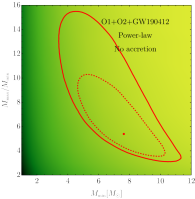
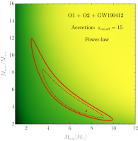
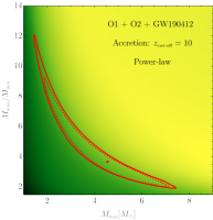
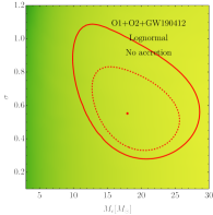
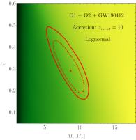
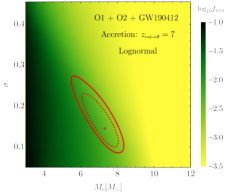
Figure 11: Likelihood on the parameter space for the power-law (top) and lognormal (bottom) mass functions requiring ${\rm N}_{\text{\tiny\rm obs}}=11$. The red dashed (solid) contours corresponds to $2\sigma$ ($3\sigma$) respectively. The leftmost panels correspond to the case in which accretion is negligible, whereas the second to fourth columns correspond to accretion suppressed at $z_{\text{\tiny\rm cut-off}}=(15,10,7)$, respectively.

In Fig. 12 we present the comparison between the initial and the final mass functions for the best-fit values obtained from the previous likelihood analysis. To highlight the differences at large masses, for the lognormal case we also show the same results in a log-linear scale. The effect of accretion is to shift the tail of the mass function to larger PBH masses, this shift being more pronounced when the accretion is stronger, with a consequent decrease of the amplitude of the peak. In other words, accretion tends to make the mass distribution broader [11]. Note, however, that the effect on the mass functions for the specific values of the parameters selected by the likelihood is much less pronounced than in the example shown in Fig. 2. This happens because the best-fit distributions peak at relatively low mass. We also notice that this evolution is for isolated PBHs, which is the relevant case for the constraints inferred from the observations other than those from GW observations. However, one should take into account that for PBHs in binaries the effect of accretion is larger, thus allowing PBH masses larger than those indicated in Fig. 12.

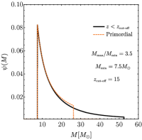
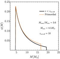
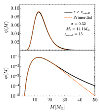
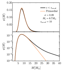
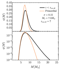
Figure 12: Primordial mass function and its evolution if accretion is present. In this plot we use the best-fit values for the parameters of the PBH mass distributions at formation, as obtained from the previous likelihood analysis. The organization of the panels is the same as in Fig. 11.

5.2 Updated constraints on PBH abundance

In Fig. 13 we present the constraints on the PBH abundance as a function of the mass, again for the best-fit values obtained from the previous likelihood analysis. In the range of masses of interest for LIGO/Virgo, the most important constraints come from lensing, dynamical processes, formation of structures, and accretion related phenomena. The lensing bounds include those from supernovae [91], the MACHO and EROS experiments [92, 93], ICARUS [94] and radio observations, such as [95] and [96] (Ogle). They all consider lensing sources at low redshift $z\ll z_{\text{\tiny cut-off}}$. Dynamical constraints involve disruption of wide binaries [97], and survival of star clusters in Eridanus II [98] and Segue I [99] at small redshifts. Bounds also arise by observations of the Lyman-$\alpha$ forest at redshift before $z\approx 4$ [100]. Other constraints involve bounds from Planck data on the CMB anisotropies induced by X-rays emitted by spherical or disk (Planck S and Planck D, respectively) [52, 101] accretion at high redshifts or bounds on the observed number of X-ray (XRay) [102, 103] and X-ray binaries (XRayB) at low redshifts [104].

In Fig. 13 we show a selection of the above constraints, identified by the nickname in parenthesis in the list above, and computed as discussed in Ref. [11]. In addition, we show the bounds coming from the absence of stochastic GW background in LIGO/Virgo data (black line) and those from the merger rate (red lines), computed as discussed in the previous section.

The red dashed and continuous lines correspond to the $2\sigma$ values for the expected number of events. In other words, the red continuous line corresponds to the upper bound from the observed merger rate, since larger values of $f_{\text{\tiny\rm PBH}}(z=0)$ would yield a merger rate higher than observed at a given mass. On the other hand, the red dashed line corresponds to a lower bound on $f_{\text{\tiny\rm PBH}}(z=0)$, assuming all the observed events are of primordial origin, since smaller values of $f_{\text{\tiny\rm PBH}}(z=0)$ would yield a merger rate lower than observed at a given mass. Clearly, this lower bound can be made less stringent by assuming that only a fraction of events is of primordial origin. The vertical dashed red lines indicate the $2\sigma$ interval around the best-fit value of the mass parameter, as obtained by the likelihood analysis.

When accretion gets stronger (for masses around $\approx 10M_{\odot}$), we observe two main effects:

• In the leftmost part of the red curve (i.e. on the left of the minimum) the GW bounds on $f_{\text{\tiny\rm PBH}}$ become more stringent, since accretion enhances the merger rate in that region. The opposite is true on the right of the minimum, because in that region accretion pushes the masses to large values, outside the optimal sensitivity range of the detectors.

• the non-GW bounds become weaker, due to the broadening of the mass function and the evolution of $f_{\text{\tiny\rm PBH}}(z)$. The interested reader can find a more detailed discussion of this phenomenon in Ref. [11].

The net result is that, if accretion is negligible, in the range of the mass-function parameters selected by the likelihood analysis, non-GW constraints (in particular Planck D) would already marginally exclude the possibility that all BH merger events detected so far are of primordial origin. However, when accretion is significant the opposite is true: LIGO/Virgo constraints are the most stringent ones in the relevant mass range. Overall, the upper bound on the PBH abundance coming from LIGO/Virgo rates is $f_{\text{\tiny\rm PBH}}(z)\lesssim{\rm few}\times 10^{-3}$ in the relevant mass range, with the upper bound becoming more stringent in the case of strong accretion. Moreover, in the relevant mass range existing constraints seem to exclude the possibility to detect the GW stochastic background from PBH mergers, because detecting the latter would require a PBH abundance which is already excluded.

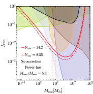
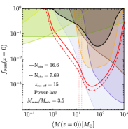
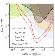
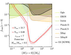
Figure 13: Constraints on $f_{\text{\tiny\rm PBH}}$ from experiments not related to GWs (see legend and main text), absence of stochastic GW background in LIGO O2 (black-solid), and upper (red-solid indicating the 2$\sigma$ exclusion region) and lower (red-dashed, obtained assuming that all BH merger events detected so far are primordial) bounds coming from the observed merger rates. As in Figs. 11 and 12, the leftmost panels correspond to the case in which accretion is negligible, whereas the second to fourth columns correspond to accretion suppressed at $z_{\text{\tiny\rm cut-off}}=(15,10,7)$, respectively.

5.3 Confrontation of the predicted distributions of the binary parameters with observations

In Fig. 14 we show the observable distribution of the chirp mass ${\cal M}\equiv\mu^{3/5}M_{\text{\tiny tot}}^{2/5}$ obtained using the the best-fit values calculated from the previous likelihood analysis and compared to LIGO/Virgo data. We have plotted the differential $R_{\text{\tiny det}}$, i.e. the number of events in the chirp mass bin normalised with respect to the total number of events (red lines). The blue histograms indicate the distribution inferred from the data. They have been obtained by plotting, in each chirp mass bin, the integral of the posterior probability summed over all measurements in that bin. On the top of the figures we have shown the individual posterior probability for each measured event. One can appreciate that the larger the accretion, the wider the distribution becomes because the high-mass tail gets more spread. For the power-law mass function, accretion shifts the peak of the distribution to smaller masses because the likelihood prefers smaller $M_{\text{\tiny min}}$. For the same reason, for very strong accretion the predicted distribution has also support for small chirp masses. For the extreme case $z_{\text{\tiny cut-off}}=7$ and a power-law distribution, the predicted merger rate at small chirp mass seems in tension with current observations.

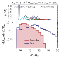
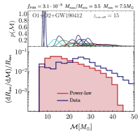
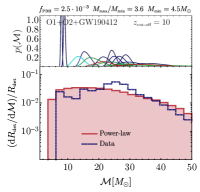
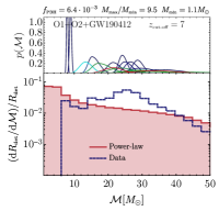
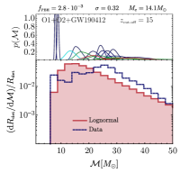
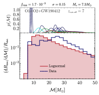
Figure 14: Observable distribution of chirp mass ${\cal M}$ (red histogram) compared to the data available (blue histogram). The organization of the panels is the same as in Fig. 13.

Fig. 15 is analogous to Fig. 14 but for the observable distribution of the mass ratio parameter $q$. Again, the histograms (blue lines) inferred from the data have been obtained by summing up, in each $q$ bin, the data weighted by the corresponding posterior probability.

Here we notice that the distributions, when accretion is included, move towards $q=1$. This is predicted by the the discussion in Sec. 2.4, where we showed that $q=1$ is a fixed-point of the binary evolution.

Current observed rates have a peak at about $q\approx 0.7$. However, it is important to note that current errors on the mass ratio (especially for LIGO/Virgo O1 and O2 events [1]) are quite large. In fact, all O1 and O2 events are compatible with $q\approx 1$; GW190412 is the only BH merger detected by LIGO/Virgo to date which has a mass ratio significantly different from unity, as also shown in the posterior distributions on the small top panels of Fig. 15. Overall, one might expect that the distributions of $q$ will change significantly as new events in O3 become available. Nonetheless, a general qualitative result can be drawn: extreme accretion scenarios (like $z_{\text{\tiny cut-off}}\lesssim 7$) are in tension with GW190412, since they would predict that the vast majority of events should have $q\sim 1$. Furthermore, the cases of a power-law and a lognormal mass functions with $z_{\text{\tiny cut-off}}\simeq 10$, see Fig. 14, which seemed to be in good agreement as far as the chirp mass distribution is concerned, seem to be in tension with the corresponding mass-ratio distributions. This is of course only a preliminary result which should wait for confirmation or disproval when the new flow of data will be available.

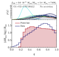
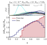
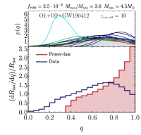
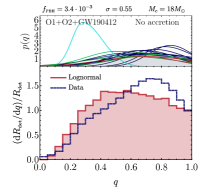
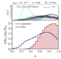
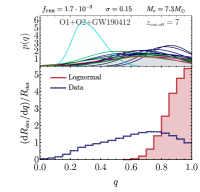
Figure 15: Same as Fig. 14, but for the observable distribution of mass ratio $q$ compared to the data available.

Finally, let us now turn our attention to the distributions of the binary spins. In Fig. 16 we plot the observable distributions of the individual spins as a function of $q$ with the same color code chosen to reflect the 1-, 2- and 3-$\sigma$ regions of Fig. 8. For each bin in $q$ we have simulated a number of binaries and built a distribution weighting the individual contributions by the relative detection rates. Notice that for the less massive PBH component of the binary, the corresponding spin $\chi_{2}$ is always larger than the spin $\chi_{1}$ of the more massive component. This is predicted by the spin evolution described in Sec. 2.4.2 and is due to the fact that $\dot{m}_{2}$ is increased by a factor $q^{-1/2}$ with respect to $\dot{m}_{1}$. Also, for large values of $q$, the magnitude of the spin $\chi_{1}$ increases when accretion becomes stronger (smaller $z_{\text{\tiny cut-off}}$), showing a strong correlation between large values of $q$ and the spins.

It is interesting to note that at least one of the components of GW190412 is moderately spinning. Indeed, assuming priors that are uniform in the spin magnitudes and isotropic in the directions, the LIGO/Virgo collaboration estimated $\chi_{1}=0.43^{+0.16}_{-0.26}$, while $\chi_{2}$ is essentially unconstrained. On the other hand, using astrophysically-motivated priors, Ref. [107] has imposed a non-spinning primary component and a uniform prior on ${\vec{\chi}_{2}}\cdot{\hat{L}}$, inferring ${\vec{\chi}_{2}}\cdot{\hat{L}}=0.88^{+0.11}_{-0.24}$. The latter can also be used as an estimate on $\chi_{2}$, assuming the orbit is not significantly tilted by the natal kick during the supernovae that produced the secondary. As shown in Fig. 16, both cases inferred by the analyses of Refs. [2, 107] are incompatible with a primordial origin for GW190412 unless: (i) accretion is significant during the cosmic history of PBHs; (ii) PBHs can be formed with non-negligible natal spin (as in some scenarios [27, 28]), in contrast with the most likely formation scenarios [25], in which the spin is at the percent level; (iii) GW190412 is actually a higher-generation merger [29], in which the spinning binary underwent a previous merger in the past. This possibility has been recently explored in Refs. [108, 109, 110], under the hypothesis that GW190412 originates from first-generation or hierarchical mergers of astrophysical origin in the context of both the field and cluster formation scenarios. However, in the case of PBHs the possibility of hierarchical merger is less likely, since the merger rates for higher-generation mergers are much smaller than those of first-generation mergers [30, 31, 12]. The possibility that GW190412 was a higher-generation merger (of either astrophysical or primordial origin) requires a better assessment of its spin and a comparison with multiple-generation scenarios. A robust assessment will probably require to wait for more events like GW190412 in O3 or future observational runs.

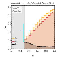
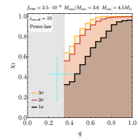
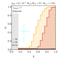
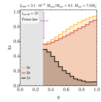
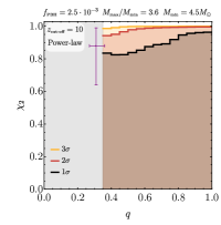
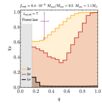
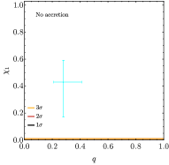
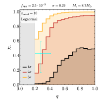
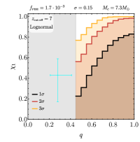
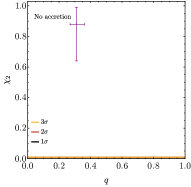
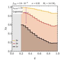
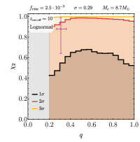
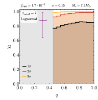
Figure 16: Observable distribution of the individual spins as a function of $q$ for the power-law (first two blocks) and the lognormal (last two blocks) mass functions. The cyan data point refers to the measurement of $\chi_{1}$ for GW190412 provided in Ref. [2], whereas the purple data point to the measurement of $\chi_{2}$ for the same system as provided in Ref. [107] (where a prior $\chi_{1}=0$ was imposed). The grey bands indicate those regions where the PBH model does not provide a number of observable events with a sufficiently high statistical significance.

Finally, in Fig. 17 we plot the observable distribution of the effective spin as a function of $q$ compared to the data available. These plots show, when accretion is important, a strong correlation between $\chi_{\text{\tiny eff}}$ and $q$. Obviously, in the case of no accretion, the effective spin parameter is vanishing, owing to the initial conditions of the individual spins.

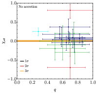
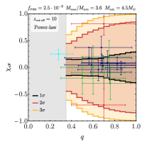
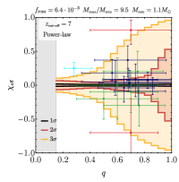
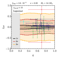
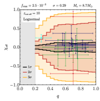
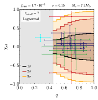
Figure 17: Observable distribution of the effective spin as a function of $q$ compared to the data available for the power-law (first block) and the lognormal (last block) mass functions. The structure of the panels and the grey bands have the same meaning as in Fig. 16.

6 Conclusions: Key predictions of the PBH scenario for GW astronomy

With the current and upcoming wealth of data on BH binaries from the LIGO/Virgo observatories, it becomes possible to perform model selection and rule out or corroborate specific formation scenarios for BHs in the LIGO/Virgo band. We have investigated whether current data – including O1, O2 and the recently discovered GW190412 – are compatible with the hypothesis that LIGO/Virgo BHs are of primordial origin.

We conclude by summarising our main findings and listing the main predictions of the PBH scenario, which can be directly tested with current and future GW observations:

1. For a given PBH mass distribution at formation, current merger rates set an upper bound on the PBH abundance at the level of $f_{\text{\tiny\rm PBH}}\mathrel{\hbox to0.0pt{\lower 4.0pt\hbox{\hskip 0.5pt$\sim$}\hss}\raise 1.0pt\hbox{$<$}}(10^{-2}\div 10^{-3})$, depending on the mass function. The best-fit values selected by the likelihood provide mass distributions which are optimally compatible with current events. For the case of a lognormal distribution and no accretion, our best-fit parameters are in agreement with the recent analysis in Ref. [90] within $1\sigma$. In addition, we found that accretion can alter quantitatively the distributions, but not the qualitative aspects of this analysis.

2. Although not directly relevant for the LIGO/Virgo frequency range, it is intriguing that accretion can be very efficient for PBHs with initial mass $M^{\text{\tiny i}}\gtrsim 10M_{\odot}$, increasing the latter by some orders of magnitude during the cosmic history. Thus, it might occur that PBHs formed with masses $\sim(10\div 100)M_{\odot}$ can have much larger masses when detected at smaller redshift. These objects would be natural candidates for intermediate-mass BHs, which are sources for ET and LISA. If these objects were born in the stellar-mass range in the primordial universe, they should also have nearly-extremal spin and mass ratio close to unity.

3. The fact that at least one of the components of GW190412 is moderately spinning is incompatible with a primordial origin for this event, unless: (i) PBHs are born with non-negligible spin, in contradiction with the most likely formation scenarios; (ii) at least the spinning component of GW190412 is a second-generation BH (however, this would require a better assessment of its spin and a comparison with multiple-generation merger scenarios, which are unlikely for PBHs [12]); (iii) accretion is significant during the cosmic history of PBHs.

4. Despite the uncertainties in the accretion modelling, the role of accretion onto PBHs is manifold. Due to the effect of super-Eddington accretion at $z\approx 30$, and to the fact that accretion onto the smaller binary component is stronger than on the primary, the mass ratio of PBH binaries with total mass above a transition value, $M_{\text{\tiny tot}}\mathrel{\hbox to0.0pt{\lower 4.0pt\hbox{\hskip 0.5pt$\sim$}\hss}\raise 1.0pt\hbox{$>$}}10M_{\odot}$ tends to be close to unity. The precise value of the transition depends on the cut-off redshift at which accretion ceases to be efficient. This produces a peculiar distribution of the binary chirp mass (Fig. 14) and mass ratio (Fig. 15), which is absent in the stellar-origin scenario. However, for the best-fit values of the lognormal distribution, the effect of accretion on the expected distribution of $q$ for the detected events is small.

5. Overall, in the case of efficient accretion the spins of the binary components at detection are non-negligible and can be close to extremality for individual PBH with final masses $M^{\text{\tiny i}}\mathrel{\hbox to0.0pt{\lower 4.0pt\hbox{\hskip 0.5pt$\sim$}\hss}\raise 1.0pt\hbox{$>$}}(10\div 30)M_{\odot}$. The transition value depends on the initial mass ratio and on the cut-off redshift.

6. For the same reason as above, assuming PBHs are formed with negligible angular momentum, the spin of the smaller binary component at detection is always higher than the one of the primary, unless hierarchical mergers occur (which are, however, unlikely [12]).

7. In all cases, the final spin of the secondary is close to extremality if the mass of the primary $M_{1}\mathrel{\hbox to0.0pt{\lower 4.0pt\hbox{\hskip 0.5pt$\sim$}\hss}\raise 1.0pt\hbox{$>$}}40M_{\odot}$.

8. It is worth noting that – if accretion is inefficient – current non-GW constraints (in particular from the absence of extra CMB distortions [52, 101]) already exclude that LIGO/Virgo events are all of primordial origin, whereas in the presence of accretion the GW bounds on the PBH abundance are the most stringent ones in the relevant mass range.

9. Overall, a strong phase of accretion during the cosmic history would favour mass ratios close to unity, and a redshift-dependent correlation between high PBH masses, high spins, and $q\approx 1$. These correlations can be used to distinguish the accreting PBH scenario from that of astrophysical-origin BH binaries.

10. Extreme accretion scenarios (in our study represented by $z_{\text{\tiny cut-off}}\lesssim 7$) predict that most of the events should be clustered around $q\sim 1$. This is in tension with the recent GW190412 data.

11. The individual spin evolution results in a broad distribution of the effective spin parameter of the binary, which is compatible with the observed distribution of the GW events detected so far [112, 1, 49, 50, 51], including GW190412 [2]. In particular, in the accreting PBH scenario the dispersion of $\chi_{\text{\tiny eff}}$ around zero grows with the mass (as GW data suggest [113]), with a dispersion $\approx 0$ for low binary masses and ${\cal O}(1)$ at larger masses.

12. The above properties produce a peculiar distribution of $\chi_{i}$ and $\chi_{\text{\tiny eff}}$ as a function of the mass ratio (Figs. 16 and 17), which is absent in the stellar-origin scenario.

13. According to our theoretical predictions, low mass PBHs, $M\mathrel{\hbox to0.0pt{\lower 4.0pt\hbox{\hskip 0.5pt$\sim$}\hss}\raise 1.0pt\hbox{$<$}}{\cal O}(10)M_{\odot}$, should have tiny spins. This property might help to distinguish PBH binaries from those composed by neutron stars [114], in the case the spin of the latter is non-negligible.

It is worth mention that – in confronting our theoretical predictions with GW observations – we have relied on the measurements obtained by the LIGO/Virgo collaboration. The latter are based on agnostic priors on the masses and spins. A different choice of the priors – possibly motivated by a sound PBH scenario – might affect the posterior distributions of the observed parameters, especially for those which are poorly measured (see Ref. [107] for an example in the context of astrophysical priors for the spin of GW190412). We plan to investigate this interesting problem in a future work [115].

Furthermore, given the important role that accretion on PBHs can play in the phenomenology of GW coalescence events and in relaxing current constraints on the PBH abundance, we advocate the urgent need of a better modelling of the accretion rate at redshift $z\lesssim 30$.

Finally, the question whether the PBHs may be responsible or not of the LIGO/Virgo data has the following answer: while in the absence of accretion the LIGO/Virgo events are incompatible with the primordial nature of BHs, the situation – in the presence of accretion – is at the moment not conclusive, even though the theoretical predictions of the PBH scenario are rather sharp. The next forthcoming data from the O3 campaign and from the Advanced LIGO might provide a more definite answer.

References

- [1] B. P. Abbott et al. [LIGO Scientific and Virgo Collaborations], Phys. Rev. X 9, no. 3, 031040 (2019) [astro-ph.HE/1811.12907].
- [2] R. Abbott et al. [LIGO Scientific and Virgo], [astro-ph.HE/2004.08342].
- [3] L. Barack et al., Class. Quant. Grav. 36 (2019) no.14, 143001 [gr-qc/1806.05195].
- [4] M. Sasaki, T. Suyama, T. Tanaka and S. Yokoyama, Class. Quant. Grav. 35, no. 6, 063001 (2018) [astro-ph.CO/1801.05235].
- [5] S. Bird, I. Cholis, J. B. Muñoz, Y. Ali-Haïmoud, M. Kamionkowski, E. D. Kovetz, A. Raccanelli and A. G. Riess, Phys. Rev. Lett. 116, no. 20, 201301 (2016) [astro-ph.CO/1603.00464].
- [6] M. Sasaki, T. Suyama, T. Tanaka and S. Yokoyama, Phys. Rev. Lett. 117, no. 6, 061101 (2016) Erratum: [Phys. Rev. Lett. 121, no. 5, 059901 (2018)] [astro-ph.CO/1603.08338].
- [7] B. Carr, K. Kohri, Y. Sendouda and J. Yokoyama, [astro-ph.CO/2002.12778].
- [8] M. Ricotti, Astrophys. J. 662, 53 (2007) [astro-ph/0706.0864].
- [9] M. Ricotti, J. P. Ostriker and K. J. Mack, Astrophys. J. 680, 829 (2008) [astro-ph/0709.0524].
- [10] J. R. Rice and B. Zhang, JHEAp 13-14, 22 (2017) [astro-ph.HE/1702.08069].
- [11] V. De Luca, G. Franciolini, P. Pani and A. Riotto, [astro-ph.CO/2003.12589].
- [12] V. De Luca, G. Franciolini, P. Pani and A. Riotto, JCAP 04 (2020), 052 [astro-ph.CO/2003.02778].
- [13] B. J. Carr, Astrophys. J. 201 (1975), 1-19
- [14] C. T. Byrnes, M. Hindmarsh, S. Young and M. R. S. Hawkins, JCAP 08 (2018), 041 [astro-ph.CO/1801.06138].
- [15] C. T. Byrnes, P. S. Cole and S. P. Patil, JCAP 06 (2019), 028 [astro-ph.CO/1811.11158].
- [16] V. De Luca, G. Franciolini and A. Riotto, [astro-ph.CO/2001.04371].
- [17] A. Dolgov and J. Silk, Phys. Rev. D 47 (1993), 4244-4255
- [18] B. Carr, M. Raidal, T. Tenkanen, V. Vaskonen and H. Veermäe, Phys. Rev. D 96, no. 2, 023514 (2017) [astro-ph.CO/1705.05567].
- [19] J. M. Bardeen, J. Bond, N. Kaiser and A. Szalay, Astrophys. J. 304 (1986), 15-61
- [20] S. Blinnikov, A. Dolgov, N. K. Porayko and K. Postnov, JCAP 1611, 036 (2016) [astro-ph.HE/1611.00541].
- [21] J. García-Bellido, J. Phys. Conf. Ser. 840, no. 1, 012032 (2017) [astro-ph.CO/1702.08275].
- [22] P. Ivanov, P. Naselsky and I. Novikov, Phys. Rev. D 50, 7173 (1994).
- [23] J. García-Bellido, A.D. Linde and D. Wands, Phys. Rev. D 54 (1996) 6040 [astro-ph/9605094].
- [24] P. Ivanov, Phys. Rev. D 57, 7145 (1998) [astro-ph/9708224].
- [25] V. De Luca, V. Desjacques, G. Franciolini, A. Malhotra and A. Riotto, JCAP 05 (2019), 018 [astro-ph.CO/1903.01179].
- [26] M. Mirbabayi, A. Gruzinov and J. Noreña, JCAP 03 (2020), 017 [astro-ph.CO/1901.05963].
- [27] T. Harada, C. M. Yoo, K. Kohri and K. I. Nakao, Phys. Rev. D 96, no. 8, 083517 (2017) Erratum: [Phys. Rev. D 99, no. 6, 069904 (2019)] [gr-qc/1707.03595].
- [28] E. Cotner and A. Kusenko, Phys. Rev. D 96 (2017) no.10, 103002 [astro-ph.CO/1706.09003].
- [29] D. Gerosa and E. Berti, Phys. Rev. D 95, no. 12, 124046 (2017) [gr-qc/1703.06223].
- [30] L. Liu, Z. K. Guo and R. G. Cai, Eur. Phys. J. C 79 (2019) no.8, 717 [astro-ph.CO/1901.07672].
- [31] Y. Wu, Phys. Rev. D 101, no.8, 083008 (2020) [astro-ph.CO/2001.03833].
- [32] S. L. Shapiro and S. A. Teukolsky Black holes, white dwarfs, and neutron stars: The physics of compact objects (Wiley, 1983).
- [33] J. Adamek, C. T. Byrnes, M. Gosenca and S. Hotchkiss, Phys. Rev. D 100 (2019) no.2, 023506 [astro-ph.CO/1901.08528].
- [34] K. J. Mack, J. P. Ostriker and M. Ricotti, Astrophys. J. 665, 1277 (2007) [astro-ph/0608642].
- [35] Poisson, E. and Will, C.M., Gravity: Newtonian, Post-Newtonian, Relativistic, (2014), Cambridge University Press.
- [36] E. Berti and M. Volonteri, Astrophys. J. 684, 822 (2008) [astro-ph/0802.0025].
- [37] P. Pani and A. Loeb, Phys. Rev. D 88, 041301 (2013) [astro-ph.CO/1307.5176].
- [38] R. Brito, V. Cardoso and P. Pani, Lect. Notes Phys. 906, pp.1 (2015) [gr-qc/1501.06570].
- [39] J. P. Conlon and C. A. R. Herdeiro, Phys. Lett. B 780, 169 (2018) [astro-ph.HE/1701.02034].
- [40] A. Dima and E. Barausse, [gr-qc/2001.11484].
- [41] R. Narayan and I. Yi, Astrophys. J. 452 (1995), 710 [astro-ph/9411059].
- [42] N. Shakura and R. Sunyaev, Astron. Astrophys. 24 (1973), 337-355
- [43] Novikov, I. D. and Thorne, K. S. Astrophysics of black holes. In Black Holes (Les Astres Occlus), ed. A. Giannaras, 343–450.
- [44] J. M. Bardeen, W. H. Press and S. A. Teukolsky, Astrophys. J. 178, 347 (1972).
- [45] K. S. Thorne, Astrophys. J. 191 (1974), 507-520
- [46] R. Brito, V. Cardoso and P. Pani, Class. Quant. Grav. 32, no. 13, 134001 (2015) [gr-qc/1411.0686].
- [47] M. Volonteri, P. Madau, E. Quataert and M. J. Rees, Astrophys. J. 620, 69 (2005) [astro-ph/0410342].
- [48] C. F. Gammie, S. L. Shapiro and J. C. McKinney, Astrophys. J. 602, 312 (2004) [astro-ph/0310886].
- [49] B. Zackay, T. Venumadhav, L. Dai, J. Roulet and M. Zaldarriaga, Phys. Rev. D 100, no. 2, 023007 (2019) [astro-ph.HE/1902.10331].
- [50] T. Venumadhav, B. Zackay, J. Roulet, L. Dai and M. Zaldarriaga, [astro-ph.HE/1904.07214].
- [51] Y. Huang et al., [gr-qc/2003.04513].
- [52] Y. Ali-Haïmoud and M. Kamionkowski, Phys. Rev. D 95, no. 4, 043534 (2017) [astro-ph.CO/1612.05644].
- [53] S. Oh and Z. Haiman, Mon. Not. Roy. Astron. Soc. 346 (2003), 456 [astro-ph/0307135].
- [54] G. Hasinger, [astro-ph.CO/2003.05150].
- [55] G. Hütsi, M. Raidal and H. Veermäe, Phys. Rev. D 100, no. 8, 083016 (2019) [astro-ph.CO/1907.06533].
- [56] Y. Ali-Haïmoud, E. D. Kovetz and M. Kamionkowski, Phys. Rev. D 96, no. 12, 123523 (2017) [astro-ph.CO/1709.06576].
- [57] V. Bosch-Ramon and N. Bellomo, [astro-ph.CO/2004.11224].
- [58] D. Spergel et al. [WMAP], Astrophys. J. Suppl. 148 (2003), 175-194 [astro-ph/0302209].
- [59] N. Aghanim et al. [Planck], [astro-ph.CO/1807.06209].
- [60] M. Maggiore, “Gravitational Waves. Vol. 1: Theory and Experiments.”
- [61] A. Caputo, L. Sberna, A. Toubiana, S. Babak, E. Barausse, S. Marsat and P. Pani, [astro-ph.HE/2001.03620].
- [62] P. C. Peters and J. Mathews, Phys. Rev. 131, 435 (1963).
- [63] P. C. Peters, Phys. Rev. 136, B1224 (1964).
- [64] E. Barausse, V. Cardoso and P. Pani, Phys. Rev. D 89 (2014) no.10, 104059 [gr-qc/1404.7149].
- [65] C. F. Macedo, P. Pani, V. Cardoso and L. Crispino, C.B., Astrophys. J. 774 (2013), 48 [gr-qc/1302.2646].
- [66] L.D. Landau and E.M. Lifshitz, “Mechanics: Volume 1.”
- [67] M. Maggiore et al., [astro-ph.CO/1912.02622].
- [68] P. Amaro-Seoane et al. [LISA], [astro-ph.IM/1702.00786].
- [69] Y. Ali-Haïmoud, Phys. Rev. Lett. 121, no. 8, 081304 (2018) [astro-ph.CO/1805.05912].
- [70] V. Desjacques and A. Riotto, Phys. Rev. D 98, no. 12, 123533 (2018) [astro-ph.CO/1806.10414].
- [71] G. Ballesteros, P. D. Serpico and M. Taoso, JCAP 1810, 043 (2018) [astro-ph.CO/1807.02084].
- [72] A. Moradinezhad Dizgah, G. Franciolini and A. Riotto, JCAP 1911, no. 11, 001 (2019) [astro-ph.CO/1906.08978].
- [73] M. Raidal, C. Spethmann, V. Vaskonen and H. Veermäe, JCAP 02 (2019), 018 [astro-ph.CO/1812.01930].
- [74] P. Ajith et al., Phys. Rev. D 77, 104017 (2008) Erratum: [Phys. Rev. D 79, 129901 (2009)] [gr-qc/0710.2335].
- [75] B. Abbott et al. [KAGRA, LIGO Scientific and VIRGO], Living Rev. Rel. 21 (2018) no.1, 3 [gr-qc/1304.0670].
- [76] P. Ajith et al., Phys. Rev. Lett. 106, 241101 (2011) [gr-qc/0909.2867].
- [77] D. A. Hemberger, G. Lovelace, T. J. Loredo, L. E. Kidder, M. A. Scheel, B. Szilágyi, N. W. Taylor and S. A. Teukolsky, Phys. Rev. D 88, 064014 (2013) [gr-qc/1305.5991].
- [78] L. S. Finn and D. F. Chernoff, Phys. Rev. D 47 (1993), 2198-2219 [gr-qc/9301003].
- [79] E. Berti, A. Buonanno and C. M. Will, Phys. Rev. D 71, 084025 (2005) [gr-qc/0411129].
- [80] M. Dominik et al., Astrophys. J. 806, no. 2, 263 (2015) [astro-ph.HE/1405.7016].
- [81] Z. C. Chen and Q. G. Huang, Astrophys. J. 864 (2018) no.1, 61 [astro-ph.CO/1801.10327].
- [82] M. Raidal, V. Vaskonen and H. Veermäe, JCAP 1709, 037 (2017) [astro-ph.CO/1707.01480].
- [83] S. Wang, Y. F. Wang, Q. G. Huang and T. G. F. Li, Phys. Rev. Lett. 120, no. 19, 191102 (2018) [astro-ph.CO/1610.08725].
- [84] X. J. Zhu, E. Howell, T. Regimbau, D. Blair and Z. H. Zhu, Astrophys. J. 739, 86 (2011) [gr-qc/1104.3565].
- [85] Z. C. Chen, F. Huang and Q. G. Huang, Astrophys. J. 871, no. 1, 97 (2019) [gr-qc/1809.10360].
- [86] E. Thrane and J. D. Romano, Phys. Rev. D 88, no. 12, 124032 (2013) [astro-ph.IM/1310.5300].
- [87] B. P. Abbott et al. [LIGO Scientific and Virgo Collaborations], Phys. Rev. Lett. 116, no. 13, 131102 (2016) [gr-qc/1602.03847].
- [88] A. D. Gow, C. T. Byrnes, A. Hall and J. A. Peacock, JCAP 01 (2020) no.01, 031 [astro-ph.CO/1911.12685].
- [89] N. Fernandez and S. Profumo, JCAP 08, 022 (2019) [astro-ph.HE/1905.13019].
- [90] A. Dolgov, A. Kuranov, N. Mitichkin, S. Porey, K. Postnov, O. Sazhina and I. Simkin, [astro-ph.CO/2005.00892].
- [91] M. Zumalacarregui and U. Seljak, Phys. Rev. Lett. 121, no. 14, 141101 (2018) [astro-ph.CO/1712.02240].
- [92] C. Alcock et al. [MACHO Collaboration], Astrophys. J. Suppl. 136, 439 (2001) [astro-ph/0003392]
- [93] R. A. Allsman et al. [Macho Collaboration], Astrophys. J. 550, L169 (2001) [astro-ph/0011506].
- [94] M. Oguri, J. M. Diego, N. Kaiser, P. L. Kelly and T. Broadhurst, Phys. Rev. D 97, no. 2, 023518 (2018) [astro-ph.CO/1710.00148].
- [95] P. N. Wilkinson et al., Phys. Rev. Lett. 86, 584 (2001) [astro-ph/0101328].
- [96] H. Niikura, M. Takada, S. Yokoyama, T. Sumi and S. Masaki, Phys. Rev. D 99 (2019) no.8, 083503 [astro-ph.CO/1901.07120].
- [97] D. Quinn, M. Wilkinson, M. Irwin, J. Marshall, A. Koch and V. Belokurov, Mon. Not. Roy. Astron. Soc. 396 (2009), 11 [astro-ph.GA/0903.1644].
- [98] T. D. Brandt, Astrophys. J. 824, no. 2, L31 (2016) [astro-ph.GA/1605.03665].
- [99] S. M. Koushiappas and A. Loeb, Phys. Rev. Lett. 119, no. 4, 041102 (2017) [astro-ph.GA/1704.01668].
- [100] R. Murgia, G. Scelfo, M. Viel and A. Raccanelli, Phys. Rev. Lett. 123, no.7, 071102 (2019) [astro-ph.CO/1903.10509].
- [101] P. D. Serpico, V. Poulin, D. Inman and K. Kohri, [astro-ph.CO/2002.10771].
- [102] D. Gaggero, G. Bertone, F. Calore, R. M. T. Connors, M. Lovell, S. Markoff and E. Storm, Phys. Rev. Lett. 118 (2017) no.24, 241101 [astro-ph.HE/1612.00457].
- [103] J. Manshanden, D. Gaggero, G. Bertone, R. M. Connors and M. Ricotti, JCAP 06 (2019), 026 [astro-ph.HE/1812.07967].
- [104] Y. Inoue and A. Kusenko, JCAP 1710, 034 (2017) [astro-ph.CO/1705.00791].
- [105] V. Vaskonen and H. Veermäe, Phys. Rev. D 101 (2020) no.4, 043015 [astro-ph.CO/1908.09752].
- [106] S. Miller, T. A. Callister and W. Farr, [astro-ph.HE/2001.06051].
- [107] I. Mandel and T. Fragos, [astro-ph.HE/2004.09288].
- [108] D. Gerosa, S. Vitale and E. Berti, [astro-ph.HE/2005.04243].
- [109] C. L. Rodriguez, K. Kremer, M. Y. Grudić, Z. Hafen, S. Chatterjee, G. Fragione, A. Lamberts, M. A. Martinez, F. A. Rasio, N. Weatherford and C. S. Ye, [astro-ph.HE/2005.04239].
- [110] A. Olejak, K. Belczynski, D. Holz, J. P. Lasota, T. Bulik and M. Miller, [astro-ph.HE/2004.11866].
- [111] C. Kimball, C. Talbot, C. P. Berry, M. Carney, M. Zevin, E. Thrane and V. Kalogera, [astro-ph.HE/2005.00023].
- [112] B. P. Abbott et al. [LIGO Scientific and Virgo Collaborations], Astrophys. J. 882 (2019) no.2, L24 [astro-ph.HE/1811.12940].
- [113] M. Safarzadeh, W. M. Farr and E. Ramirez-Ruiz, [gr-qc/2001.06490].
- [114] M. Fasano, K. W. Wong, A. Maselli, E. Berti, V. Ferrari and B. S. Sathyaprakash, [astro-ph.HE/2005.01726].
- [115] S. Bhagwat, V. De Luca, G. Franciolini, P. Pani and A. Riotto, [astro-ph.CO/2008.12320].