Kibble-Zurek mechanism in a Dissipative Transverse Ising Chain

Abstract

We study the Kibble-Zurek mechanism in the transverse Ising chain coupled to a dissipative boson bath, making use of a new numerical method with the infinite time evolving block decimation combined with the discrete-time path integral. We first show the ground-state phase diagram and confirm that a quantum phase transition takes place in the presence of the system-bath coupling. Then we present the time dependence of the energy expectation value of the spin Hamiltonian and the scaling of the kink density with respect to the time period over which the spin Hamiltonian crosses a quantum phase transition. The energy of spins starts to grow from the energy at the ground state of the full system near a quantum phase transition. The kink density decays as a power law with respect to the time period. These results confirm that the Kibble-Zurek mechanism happens. We discuss the exponent for the decay of the kink density in comparison with a theoretical result with the quantum Monte-Carlo simulation. A comparison to an experimental study is also briefly mentioned.

I Introduction

When a parameter of an isolated macroscopic system is varied with a finite speed near a quantum phase transition, the system, departing from its ground state, develops into a non-trivial out-of-equilibrium state with topological defects. This spontaneous creation of inhomegeneity during the time evolution near a quantum phase transition is called the Kibble-Zurek mechanism (KZM)Kibble (1976); Zurek (1985). The most remarkable phenomenon of KZM is the universal scaling, named as the Kibble-Zurek scaling (KZS), of the density of defects with respect to the changing speed of the parameter. Intensive studies in past decades have established that, as far as a standard quantum phase transition of the second order is concerned, the density of defects obeys a power law with an exponent determined by critial exponents of the associated quantum phase transitionZurek et al. (2005); Polkovnikov (2005); Polkovnikov et al. (2011).

Compared to an isolated system, dissipative systems have not been studied thoroughly so far. Previous studies on dissipative systems have been limited to ideal free-fermion systems in one dimension with no mixing between different momentum sectors Patané et al. (2008, 2009); Nalbach et al. (2015); Dutta et al. (2016); Keck et al. (2017); Arceci et al. (2018). However, it is no doubt that dissipation is crucially important to out-of-equilibrium states in more real physical systems as well. Therefore it is significant to investigate KZM in dissipative quantum systems from more realistic point of view.

Recently, a commercialized quantum annealing machine manufactured by D-Wave Systems Inc. has received great attention. Quantum annealing was proposed to solve combinatorial optimization problems represented by the energy minimization of an interacting Ising-spin modelKadowaki and Nishimori (1998); Farhi et al. (2001). Following the standard method of quantum annealing, one applies a strong transverse field to interacting Ising spins at first and weaken it slowly with time. Then the spin state which is initialized as the trivial ground state of the transverse field evolves adiabatically, and eventually reaches the target ground state of the interacting Ising model when the transverse field vanishes. The adiabatic time evolution is guaranteed when the square of the instantaneous energy gap above the ground state is sufficiently large compared to the changing speed of the HamiltonianKato (1950); Messiah (1961). However, it has been known that a quantum phase transtition usually takes place during quantum annealing and the instantaneous energy gap vanishes at a transitionSachdev (1999). Therefore, quantum annealing is seen as a time evolution across a quantum phase transition and its performance is closely related to KZM.

D-Wave’s machine implements quantum annealing physically in its device. Although a lot of tests have been done so far to characterize the performance of the machine, its mechanism has not been fully clarified. Several studies have shown that the system embedded in D-Wave’s machine is not closed but open to a dissipative environment. D-Wave’s machine is now believed to implement quantum annealing in a dissipative system. Thus KZM in a dissipative transverse Ising model is worth studying from the viewpoint of not only out-of-equilibrium statistical mechanics but also revealing the mechanism of D-Wave’s machine.

The difficulty in theoretically studying a dissipative quantum many-body system is that there have been few good method. In order to study the time evolution of a dissipative quantum system, the Born-Markov (BM) approximation is often usedWeiss (2012). BM approximation reduces the complexity of computation, but it involves an approximation in an uncontrollable manner and one cannot improve accuracy systematically. The Lindblad formalism, which is derived with BM approximation, enables us to perform numerical computation for large systems, i.e., tens of quantum spins for instance. The approximation in the Lindblad formalism replaces the coupling to an environment with an abstract one and hence some of the features of the original system are lost completely. In the present work, we apply the infinite time evolving block decimation (iTEBD) method to the dissipative transverse Ising chain for the first time. The dissipative transverse Ising chain is mapped to a double-layered two-dimensional Ising model after tracing out the bosonic degrees of freedom. The difference from the dissipationless model is that there are long-range interactions along the time axis. The use of matrix product representation for the spin chain along the time axis enables us to utilize the iTEBD method to the dissipative model. This is essantially an extention of the method for finite system that the present authors developed recentlySuzuki et al. (2019). The present method does not rely on the BM approximation and the approximation involved is controlled by parameters. With the present method, one can study the time evolution as well as the thermal equilibrium of the translationally invariant infinite system without any finite-size effect.

Using our method, we study the equilibrium and out-of-equilibrium states of the dissipative transverse Ising chain with the Caldeira-Leggett type of the system-bath coupling. As shown in Sec. II, this model cannot be mapped to a free-fermion model and has not been studied so far in the context of KZM. We first present the ground-state phase diagram, confirming that the quantum phase transition survives in a certain range of the system-bath coupling strength. Then we investigate the scaling of the density of defects associated with the change of the Hamiltonian linear in time across a quantum phase transition. It is shown that the density of defects scales as a power law of the changing speed of the transverse field, and that the exponent diminishes gradually with increasing the strength of the system-bath coupling. The result is discussed in comparison to the previous work. We finally comment on experiments of KZM in the present model using D-Wave’s machines.

This paper is organized as follows. We specify the dissipative transverse Ising chain in the next section. In Sec. III, we describe our new method for equilibrium and out-of-equlibrium states of the dissipative transverse Ising chain based on the discrete-time path integral and iTEBD. Section IV is devoted to the presentation of our results. The ground-state phase diagram of the present model is given and KZS is discussed in detail there. This paper conludes with Sec. V.

II Model

We consider the dissipative transverse Ising chain described by the Hamiltonian

$$H=H_{\rm S}+H_{\rm B}+H_{\rm int},$$ (1)

where $H_{\rm S}$, $H_{\rm B}$ and $H_{\rm int}$ represent the transverse Ising chain, the boson bath, and the interaction between them, respectively, and given by

$$H_{\rm S}=-J\sum_{j=1}^{N-1}\sigma_{j}^{z}\sigma_{j+1}^{z}-\Gamma\sum_{j=1}^{N}\sigma_{j}^{x},$$ (2)

$$H_{\rm B}=\sum_{j=1}^{N}\sum_{a}\omega_{a}b_{ja}^{\dagger}b_{ja},$$ (3)

$$H_{\rm int}=\sum_{j=1}^{N}\sigma_{j}^{z}\sum_{a}\lambda_{a}\left(b_{ja}^{\dagger}+b_{ja}\right),$$ (4)

Here $\sigma_{j}^{c}$ ($c=x$, $z$) are the Pauli operators at site $j$, $J$ and $\Gamma$ stand for the coupling strength of Ising spins and the transverse field, respectively, and $b_{ja}^{\dagger}$ ($b_{ja}$) is the bosonic creation (annihilation) operator at site $j$ with mode $a$. We make $\hbar=1$ throughout the paper. We assume that the boson bath has the Ohmic spectral density

$$\mathcal{J}(\omega)=\sum_{a}\lambda_{a}^{2}\delta(\omega-\omega_{a})=\alpha\omega e^{-\omega/\omega_{c}},$$ (5)

where $\alpha$ is the coupling strength between the spin system and the bath, and $\omega_{c}$ is the cutoff energy of the bath spectrum which is chosen to be larger than the other energy scales. The spin-boson interaction assumed in Eq. (4) is the many spin version of the Caldeira-Leggett model for the superconducting flux qubitCaldeira and Leggett (1983); Leggett et al. (1987). The present model is the simplest and the most realistic one to study the dissipative system in D-Wave’s machine.

The presence of the system-bath coupling breaks the integrability of the transverse Ising chain, $H_{\rm S}$. The nonintegrability of the present model makes it difficult to study out-of-equilibrium states. We utilize the discrete-time path integral and infinite time evolving block decimation (iTEBD) to study the infinitely large system.

III Method

In this section, we describe the numerical method to compute the reduced density matrix and physical quantities.

III.1 Discrete-time path integral

III.1.1 Thermal equilibrium

We consider first the thermal equilibrium state of the full system. The reduced density operator for the spin subsystem is given by

$$\rho^{\rm eq}_{\rm S}(\beta)\equiv\frac{1}{Z}{\rm Tr}_{\rm B}\left(e^{-\beta H}\right),$$ (6)

where $\beta$ is the inverse temperature, $Z$ is the partition function, and ${\rm Tr}_{B}$ denotes the trace with respective to the bosonic degree of freedom. The exponential operator in RHS is arranged, using the symmetric Trotter formulaTrotter (1959); Suzuki (1986), into

$$e^{-\beta H} = \left(e^{-\Delta\tau H_{\rm int}/2}e^{-\Delta\tau(H_{\rm S}+H_{\rm B})}e^{-\Delta\tau H_{\rm int}/2}\right)^{M}+O(\Delta\tau^{2})$$ (7)

$$= e^{-\beta H_{\rm S}}e^{-\beta H_{\rm B}}e^{-\Delta\tau H_{\rm int}^{\rm I}(M\Delta\tau)/2}e^{-\Delta\tau H_{\rm int}^{\rm I}((M-1)\Delta\tau)}$$

$$\cdots e^{-\Delta\tau H_{\rm int}^{\rm I}(\Delta\tau)}e^{-\Delta\tau H_{\rm int}^{\rm I}(0)/2}+O(\Delta\tau^{2}),$$

where $M$ denotes the Trotter number, $\Delta\tau=\beta/M$, and $H_{\rm int}^{\rm I}(l\Delta\tau)$ is the interaction picture of $H_{\rm int}$ defined by

$$H_{\rm int}^{\rm I}(\tau) \equiv e^{\tau H_{\rm S}}e^{\tau H_{\rm B}}H_{\rm int}e^{-\tau H_{\rm B}}e^{-\tau H_{\rm S}}$$

$$= \sum_{j=1}^{N}e^{\tau H_{\rm S}}\sigma_{j}^{z}e^{-\tau H_{\rm S}}\sum_{a}\lambda_{a}(b_{ja}^{\dagger}e^{\omega_{a}\tau}+b_{ja}e^{-\omega_{a}\tau}).$$

Using Eqs. (7) and (III.1.1) in Eq. (6), and inserting the completeness relations between exponential operators, one obtains a path integral representation for the reduced density matrix. After performing the Gaussian integrals with respect to bosonic degree of freedom, the resultant path-integral formula of the reduced density matrix is written as

$$\langle\bm{\sigma}_{0}|\rho_{\rm S}^{\rm eq}(\beta=M\Delta\tau)|\bm{\sigma}_{M}\rangle$$ (9)

$$\approx C\sum_{\bm{\sigma}_{1}}\cdots\sum_{\bm{\sigma}_{M-1}}\prod_{j=1,N}\mathcal{F}^{\rm eq}(\sigma_{j,0},\cdots,\sigma_{j,M})$$

$$~{}~{}~{}\times\prod_{l=0}^{M}\prod_{j=1}^{N-1}\left\{\mathcal{B}^{\rm eq}(\sigma_{j,l},\sigma_{j+1,l})\right\}^{1-\frac{1}{2}\delta_{l,0}-\frac{1}{2}\delta_{l,M}},$$

where $|\bm{\sigma}_{l}\rangle$ denotes the eigenbasis of $\sigma_{j}^{z}$ satifying $\sigma_{j}^{z}|\bm{\sigma}_{l}\rangle=\sigma_{j,l}|\bm{\sigma}_{l}\rangle$, and $C$ is a normalization factor. $\mathcal{B}^{\rm eq}$ and $\mathcal{F}^{\rm eq}$ are defined by

$$\mathcal{B}^{\rm eq}(\sigma_{j,l},\sigma_{j+1,l})=\exp\left[\Delta\tau\sigma_{j,l}\sigma_{j+1,l}\right],$$ (10)

and

$$\mathcal{F}^{\rm eq}(\sigma_{j,0},\cdots,\sigma_{j,M})$$ (11)

$$=\exp\Biggl{[}\Upsilon\sum_{l=0}^{M-1}\sigma_{j,l}\sigma_{j,l+1}\Biggr{.}$$

$$~{}~{}~{}\Biggl{.}+\alpha\Delta\tau^{2}\sum_{M\geq l>m\geq 0}\mathcal{K}((l-m)\Delta\tau)\sigma_{j,l}\sigma_{j,m}\Biggr{]},$$

respectivly, where

$$\Upsilon=\frac{1}{2}\log\coth\Gamma\Delta\tau,$$ (12)

and

$$\mathcal{K}(\tau)=\int\frac{\cosh(\beta\omega/2-\tau\omega)}{\sinh\beta\omega/2}\mathcal{J}(\omega)d\omega.$$ (13)

Note that Eq. (9) represents the partition function of a $(1+1)$ dimensional Ising model with the long-range interaction in imaginary time.

III.1.2 Out of equilibrium

We next consider the time-dependent dissipative transverse Ising chain with $H_{\rm S}(t)=-J(t)\sum_{i=1}^{N-1}\sigma_{j}^{z}\sigma_{j+1}^{z}-\Gamma(t)\sum_{j=1}^{N}\sigma_{j}^{x}$, and assume the initial state being a product state between a pure spin state denoted by $|\Psi_{0}\rangle$ and the thermal equilibrium of the boson bath:

$$\rho(0)=|\Psi_{0}\rangle\langle\Psi_{0}|\bigotimes\frac{e^{-\beta H_{\rm B}}}{Z_{\rm B}},$$ (14)

where $\beta$ is the inverse temperature of the boson bath and $Z_{\rm B}={\rm Tr}_{\rm B}e^{-\beta H_{\rm B}}$.

Let $U(t)$ be the time-evolution operator that satisfies $i\frac{d}{dt}U(t)=H(t)U(t)$. The reduced density operator is written as

$$\rho_{\rm S}(t)={\rm Tr}_{\rm B}\left(U(t)\rho(0)U^{\dagger}(t)\right).$$ (15)

a In spite of the time dependence in the Hamiltonian, an algebra with the symmetric Trotter decomposition and Gaussian integrals similar to those used in the previous subsection yield the path-integral formula Makarov and Makri (1994); Suzuki et al. (2019):

$$\langle\bm{\sigma}_{M}|\rho_{\rm S}(M\Delta t)|\bm{\sigma}^{\prime}_{M}\rangle$$ (16)

$$\approx D\sum_{\bm{\sigma}_{0},\bm{\sigma}^{\prime}_{0}}\cdots\sum_{\bm{\sigma}_{M-1},\bm{\sigma}^{\prime}_{M-1}}\prod_{j=1}^{N}\mathcal{F}(\sigma_{j,0},\sigma^{\prime}_{j,0},\cdots,\sigma_{j,M},\sigma^{\prime}_{j,M})$$

$$~{}~{}~{}\times\left[\prod_{l=0}^{M}\prod_{j=1}^{N-1}\mathcal{B}_{l}(\sigma_{j,l},\sigma^{\prime}_{j,l},\sigma_{j+1,l},\sigma^{\prime}_{j+1,l})\right]\langle\bm{\sigma}_{0}|\Psi_{0}\rangle\langle\Psi_{0}|\bm{\sigma}^{\prime}_{0}\rangle$$

with

$$\mathcal{B}_{l}(\sigma_{j,l},\sigma^{\prime}_{j,l},\sigma_{j+1,l},\sigma^{\prime}_{j+1,l})$$ (17)

$$=\exp\left[i\Delta tJ_{l}\left(\sigma_{j,l}\sigma_{j+1,l}-\sigma^{\prime}_{j,l}\sigma^{\prime}_{j+1,l}\right)\right],$$

and

$$\mathcal{F}(\sigma_{j,0},\sigma^{\prime}_{j,0},\cdots,\sigma_{j,M},\sigma^{\prime}_{j,M})$$ (18)

$$=\exp\left[\sum_{j=1}^{N}\sum_{l=1}^{M}\left(\gamma_{l}\sigma_{j,l}\sigma_{j,l-1}+\gamma_{l}^{\ast}\sigma^{\prime}_{j,l}\sigma^{\prime}_{j,l-1}\right)\right.$$

$$~{}~{}~{}\left.+\alpha\Delta t^{2}\sum_{j=1}^{N}\left\{K(0)\sum_{l=0}^{M}\sigma_{j,l}\sigma^{\prime}_{j,l}-\sum_{M\geq l>m\geq 0}\left(\begin{array}[]{cc}\sigma_{j,l}&\sigma^{\prime}_{j,l}\\ \end{array}\right)\left(\begin{array}[]{cc}K((l-m)\Delta t)&-K^{\ast}((l-m)\Delta t)\\ -K((l-m)\Delta t)&K^{\ast}((l-m)\Delta t)\end{array}\right)\left(\begin{array}[]{c}\sigma_{j,m}\\ \sigma^{\prime}_{j,m}\end{array}\right)\right\}\right],$$ (24)

where $D$ is a normalization factor. The coupling parameters between Ising spins are given by

$$J_{l}=\left\{\begin{array}[]{ll}\frac{J(\Delta t)+3J(0)}{8}&\mbox{for $l=0$}\vspace{1ex}\\ \frac{3J(M\Delta t)+J((M-1)\Delta t)}{8}&\mbox{for $l=M$}\vspace{1ex}\\ \frac{J((l+1)\Delta t)+6J(l\Delta t)+J((l-1)\Delta t)}{8}&\mbox{otherwise}\end{array}\right.,$$ (25)

$$\gamma_{l}=\frac{1}{2}\log\left(-i\cot\frac{\Gamma(l\Delta t)+\Gamma((l-1)\Delta t)}{2}\Delta t\right)$$ (26)

and

$$K(t)=\int\frac{\cosh(\beta\omega/2-i\omega t)}{\sinh\beta\omega/2}\mathcal{J}(\omega)d\omega.$$ (27)

We remark that two types Ising variables, $\sigma_{j,l}$ and $\sigma^{\prime}_{j,l}$, are included in Eq. (16). This is because the reduced density operator in Eq. (15) involves the time-forward operator $U(t)$ and the time-backward one $U^{\dagger}(t)$. The former results in $\sigma_{j,l}$ and the latter in $\sigma^{\prime}_{j,l}$ in Eq. (16). Hence the effective Hamiltonian $\mathcal{H}$ represents coupled double layers of two-dimensional Ising models with nearest neighbor interactions in space and long-range interactions in time. Since the strength of the long-range interaction $K(t)$ decays with $t$, we set a cutoff $t_{c}$ in the numerical simulation so that $K(t)=0$ for $t>t_{c}$.

III.2 iTEBD

In this subsection, we briefly describe how to compute the reduced density matrix, Eq. (16), for an out-of-equilibrium state. The method mentioned here can be easily applied to the thermal equilibrium state. We hereafter use a shortened notation $S_{j,l}$ for $(\sigma_{j,l},\sigma^{\prime}_{j,l})$ in such a way that $S_{j,l}=\frac{1}{2}(1-\sigma_{j,l})+(1-\sigma^{\prime}_{j,l})$.

Using the singular value decomposition (SVD), one can write Eq. (18) in the form of a matrix product as

$$\mathcal{F}(S_{j,0},\cdots,S_{j,M})$$ (28)

$$=\sum_{\eta_{1},\cdots,\eta_{M}}\phi^{(0)S_{j,0}}_{\eta_{1}}\phi^{(1)S_{j,1}}_{\eta_{1}\eta_{2}}\cdots\phi^{(M-1)S_{j,M-1}}_{\eta_{M-1}\eta_{M}}\phi^{(M)S_{j,M}}_{\eta_{M}}.$$

The factor $\mathcal{B}_{l}$ can be represented, in a similar manner, as

$$\prod_{j=1}^{N-1}\mathcal{B}_{l}(S_{j,l},S_{j+1,l})$$ (29)

$$=\sum_{\zeta_{1},\cdots,\zeta_{N}}\Xi^{(1,l)S_{1,l}}_{\zeta_{1}}\Xi^{(2,l)S_{2,l}}_{\zeta_{1},\zeta_{2}}\cdots\Xi^{(N,l)S_{N,l}}_{\zeta_{N-1},\zeta_{N}}.$$

Finally, we write $\langle\bm{\sigma}_{0}|\Psi_{0}\rangle\langle\Psi_{0}|\bm{\sigma}^{\prime}_{0}\rangle$ as

$$\langle\bm{\sigma}_{0}|\Psi_{0}\rangle\langle\Psi_{0}|\bm{\sigma}^{\prime}_{0}\rangle$$ (30)

$$=\sum_{\mu_{1},\cdots,\mu_{N}}\Lambda^{(1,0)S_{1,0}}_{\mu_{1}}\Lambda^{(2,0)S_{2,0}}_{\mu_{1},\mu_{2}}\cdots\Lambda^{(N,0)S_{N,0}}_{\mu_{N-1},\mu_{N}}.$$

Strictly speaking, the largest matrix dimensions of $\phi^{(l)S}$ and $\Lambda^{(j,l)S}$ increase exponentially with $M$ and $N$, respectively. However, as is the case with the ground-state wave function in a one-dimensional quantum system, one can choose the basis of matrices so that the necessary information is preserved with keeping the largest matrix dimension constant in $M$ or $N$ White (2005); White and Feiguin (2004).

Let us now consider the infinite system ($N\to\infty$) with the translational invariance. In order to perform the trace over the spin degrees of freedom in Eq. (16), we exploit the iTEBD algorithm Vidal (2007); Orús and Vidal (2008). This algorithm performs the trace with respect to $\{S_{j,l}\}$ for all $j$ from $l=0$ to $l=M-1$ iteratively. After the $M$ times iteration, we obtain the infinite matrix product state (iMPS) representation of $\rho_{\rm S}(t)$, from which we can calculate physical quantities.

Hereafter, we write the $l$-th level of iMPS representation generated from the $l-1$ level as $\psi^{(l)\eta_{j,l}}_{\mu_{l},\mu^{\prime}_{l}}$, where $\eta_{j,l}$ denotes the matrix index for $\phi^{(l)S_{j,l}}$ in Eq. (28), and $\mu_{l}$ and $\mu^{\prime}_{l}$ denote matrix indices. We denote the largest matrix dimension of $\phi^{(l)S_{j,l}}$ and $\psi^{(l)\eta_{j,l}}$ by $\chi_{t}$ and $\chi_{s}$, respectively.

For $l=1$, the iMPS is given as

$$\psi^{(1)\eta_{j,1}}_{\mu_{1},\mu^{\prime}_{1}}=\sum_{S_{j,0}}\phi^{(0)S_{j,0}}_{\eta_{j,1}}\Xi^{(j,0)S_{j,0}}_{\zeta_{j,0},\zeta_{j+1,0}}\Lambda^{(0)S_{j,0}}_{\mu,\mu^{\prime}}.$$ (31)

where we define the new matrix indices as $\mu_{1}=(\zeta_{1},~{}\mu)$ and $\mu^{\prime}_{1}=(\zeta_{1},~{}\mu^{\prime})$. For $1\leq l\leq(M-2)$, the $(l+1)$-th level of iMPS is calculated by using the $l$-th one as

$$\psi^{(l+1)\eta_{j,l+1}}_{\mu_{l+1},\mu^{\prime}_{l+1}}=\sum_{S_{j,l},\eta_{j,l}}\phi^{(l)S_{j,l}}_{\eta_{j,l},\eta_{j,l+1}}\Xi^{(j,l)S_{j,l}}_{\zeta_{j,l},\zeta_{j+1,l}}\psi^{(l)\eta_{j,l}}_{\mu_{l},\mu^{\prime}_{l}}.$$ (32)

where $\mu_{l+1}=(\zeta_{j,l},~{}\mu_{l})$ and $\mu^{\prime}_{l+1}=(\zeta_{j,l},~{}\mu_{l}^{\prime})$. For each step, one can keep the matrix dimension up to $\chi_{s}$ by means of the truncation algorithm in iTEBD. The fianl iMPS is calculated as

$$\psi^{S_{j,M}}_{\mu_{M+1},\mu^{\prime}_{M+1}}=\sum_{\eta_{j,M}}\phi^{(M)S_{j,M}}_{\eta_{j,M}}\Xi^{(j,M)S_{j,M}}_{\zeta_{j,M},\zeta_{j+1,M}}\psi^{(M)\eta_{j,M}}_{\mu_{M},\mu^{\prime}_{M}}.$$ (33)

Thus the reduced density matrix is given in terms of iMPS as

$$\langle\bm{\sigma}_{M}|\rho_{\rm S}(M\Delta t)|\bm{\sigma}^{\prime}_{M}\rangle={\rm tr}[\cdots\psi^{S_{j,M}}\psi^{S_{j+1,M}}\cdots],$$ (34)

where ${\rm tr}$ denotes the matrix trace. The expectation values of physical quantities are obtained in terms of $\psi^{S}$ as follows. Redefining $\psi^{S}$ and $\tilde{\psi}\equiv\psi^{S=0}+\psi^{S=3}$ in such a way that the largest eigenvalue of $\tilde{\psi}$ is unity, the magnetization is given by

$${\rm Tr}_{\rm S}\left[\sigma^{c}\rho_{\rm S}(M\Delta t)\right] = \lim_{N\to\infty}{\rm tr}\left[\Bigl{(}\sum_{\sigma,\sigma^{\prime}}\langle\sigma|\sigma^{c}|\sigma^{\prime}\rangle\psi^{S(\sigma,\sigma^{\prime})}\Bigr{)}(\tilde{\psi})^{N}\right]$$ (35)

$$= \vec{v}^{\,t}_{\rm L}\left(\sum_{\sigma,\sigma^{\prime}}\langle\sigma|\sigma^{c}|\sigma^{\prime}\rangle\psi^{S(\sigma,\sigma^{\prime})}\right)\vec{v}_{\rm R},$$

where $\vec{v}^{\,t}_{\rm L}$ and $\vec{v}_{\rm R}$ are the left and right eigenvector of $\tilde{\psi}$ for the unit eigenvalue that satisfy the normalization condition $\vec{v}^{\,t}_{\rm L}\vec{v}_{\rm R}=1$. The correlation function is given by

$${\rm Tr}_{\rm S}\left[\sigma_{0}^{c}\sigma_{r}^{c}\rho_{\rm S}(M\Delta t)\right]$$ (36)

$$=\vec{v}^{\,t}_{\rm L}\left(\sum_{\sigma,\sigma^{\prime}}\sum_{\tau,\tau^{\prime}}\langle\sigma|\sigma_{0}^{c}|\sigma^{\prime}\rangle\langle\tau|\sigma_{r}^{c}|\tau^{\prime}\rangle\psi^{S(\sigma,\sigma^{\prime})}(\tilde{\psi})^{r-1}\psi^{S(\tau,\tau^{\prime})}\right)\vec{v}_{\rm R}.$$

Equations (35) and (36) are used to compute expectations of physical quantities.

IV Results

In order to study properties of the dissipative transverse Ising chain in and out of equilibrium, we introduce a parameter $s$ for the system Hamiltonian, so that $J=s$ and $\Gamma=1-s$, as

$$H_{\rm S}(s)=-s\sum_{i}\sigma^{z}_{i}\sigma^{z}_{i+1}-(1-s)\sum_{i}\sigma^{x}_{i}.$$ (37)

This Hamiltonian reduces to the decoupled spins in a transverse field when $s=0$, while it corresponds to the Ising model when $s=1$. In the absence of coupling to the bath, the ground state of $H_{\rm S}(s)$ is an ordered one for $\frac{1}{2}<s<1$, a disoredered one for $0\leq s<\frac{1}{2}$, and quantum critical at $s=\frac{1}{2}$. The Hamiltonian of the full system is given by $H=H_{\rm S}(s)+H_{\rm B}+H_{\rm int}$. We will focus on the zero-temperature phase diagram of the full system in the next subsection and then move to the time evolution in Sec. IV.2.

IV.1 Phase diagram

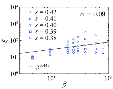
Figure 1: (a) The longitudinal-spin correlation function of the dissipative transverse Ising chain with $s=0.4$ and $\alpha=0.09$ at $\beta=40$. The correlation function decays exponentially with separation between spins. One can extract the correlation length from this behavior. (b) The correlation length $\xi$ as a function of the inverse temperatue $\beta$ for $\alpha=0.09$ and several $s$. One can find the location $s_{c}$ of the quantum critical point from the power-law growth of $\xi$ for sufficiently large $\beta$. In fact, one finds $s_{c}\approx 0.40$ for $\alpha=0.09$ from the figure. The parameters for numerical simulations were chosen as $\Delta\tau=0.05$, $\chi_{t}=128$, $\chi_{s}=128$, and $\omega_{c}$ = 5.

Consider that the full system is in the thermal equilibrium with the inverse temperature $\beta$. The reduced density operator is given by Eq. (6) and the correlation function with respect to the longitudinal spin is given by

$$C^{z}(r)={\rm Tr}_{\rm S}\left[\sigma_{0}^{z}\sigma_{r}^{z}\rho_{\rm S}^{\rm eq}(\beta)\right].$$ (38)

It is expected that, since the longitudinal spin is disordered in the equilibrium at a finite temperature, the correlation function decays exponentially for sufficiently large $r$ as

$$C^{z}(r)\sim e^{-r/\xi},$$ (39)

where $\xi$ represents the correlation length. Figure 1(a) demonstrates an exponential decay of $C^{z}(r)$ obtained by the iTEBD simulation.

Based on the ansatz of Eq. (39), we estimate the correlation length from the correlation function by

$$\xi=-\lim_{r\to\infty}\frac{r}{\log C^{z}(r)}.$$ (40)

With lowering the temperature, the correlation length obeys the scaling relation to $\beta$ depending upon the property of the ground state. When the ground state is disordered, the correlation length becomes constant with respect to the temperature. When the ground state is ordered, on the other hand, the correlation length diverges exponentially as $\xi\sim e^{a\beta}$ as $\beta\to\infty$ with a constant $a$. Finally, a quantum critical ground state bears a power-law scaling, $\xi\sim\beta^{1/z}$, where $z$ is the dynamical critical exponent. We show results on $\xi$ for several $s$ in Fig. 1(b). One can see that $\xi$ grows faster than a power law with $\beta$ for sufficiently large $s$’s, while it looks converging for smaller $s$’s. At a certain critical value of $s$ in between, $\xi$ behaves as a power law of $\beta$, from which one can determine the location of the quantum critical point $s_{c}$ for a fixed system-bath coupling $\alpha$.

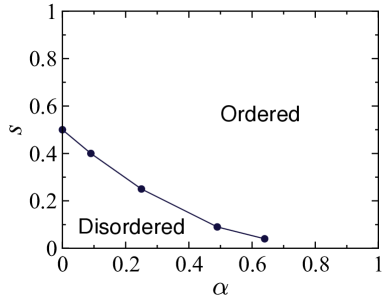
Figure 2: Ground-state phase diagram of the dissipative transverse Ising chain. With increasing the system-bath coupling, the ordered phase extends down to a smaller critical value of $s$.

Thus we show the ground-state phase diagram of the dissipative Transverse Ising chain in Fig. 2. Note that, at $\alpha=0$, the transverse Ising chain is isolated from the bath and the critical point $s=\frac{1}{2}$ is exactly known. One finds that the critical point declines with increasing the system-bath coupling and the ordered phase extends down to a smaller $s$. Although our numerical method becomes unreliable for $\alpha>0.64$, previous studies have revealed that when $s=0$ an order-disorder transition takes place at $\alpha\approx 0.625$ for $\omega_{c}=10$ and at larger $\alpha$ for smaller $\omega_{c}$ Leggett et al. (1987); Bulla et al. (2003); Werner et al. (2005); Strathearn et al. (2018). This implies that the critical line should terminate at $\alpha$ larger than 0.625 and $s=0$. Our results for $\omega_{c}=5$ are perfectly consistent to the previous studies.

Quantum critical properties of the dissipative transverse Ising chain have been studied earlier by Werner et al. using the quantum Monte-Carlo (QMC) simulation for an effective model Werner et al. (2005). They have found that the critical exponents $(\nu,z)$ associated with the quantum phase transition change from $(1,1)$ to $(0.63,2.0)$ by introducing an infinitesimal system-bath coupling $\alpha$ and do not vary on the critical line. As for our simulation, the exponent $z$ can be evaluated from the power law of $\xi$ when $s$ is fixed at a quantum critical point. The result is in fact $\frac{1}{z}\approx 0.46$ for $\alpha=0.09$, which is in reasonable agreement with $\frac{1}{2}$ from the QMC simulation.

It should be noted that the parameters involved in the QMC simulation are defined for an effective model with the unit Trotter imaginary-time step, i.e., $\Delta\tau=1$. Therefore there is not necessarily a quantitative consistency among the phase diagrams given in ref.Werner et al. (2005) and Fig. 2.

IV.2 Time evolution across a quantum phase transition

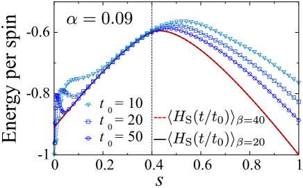
Figure 3: Time dependence of the energy expectation value of the spin Hamiltonian $H_{\rm S}(t/t_{0})$ for various $t_{0}$ and the system-bath coupling fixed at $\alpha=0.09$. The solid lines show the instantaneous energy expectation values of the thermal equilibria, $\rho_{\rm S}^{\rm eq}(\beta)$, with $\beta=40$ and $20$. Since the difference between these two lines is invisible, we consider that the solid line represents the ground state. As for the time evolution, the initial state is assumed to be the product state of the ground state of the spin system and that of the boson system. The dashed vertical line shows the location of the quantum phase transition. After an initial relaxation, the state follows the ground state but starts to deviate from the ground state near the quantum phase transition. The parameters for numerical simulations were chosen as $\Delta t=0.05$, $\chi_{t}=128$, $\chi_{s}=128$, and $\omega_{c}=5$.

Having obtained the ground state phase diagram, we next focus on the time evolution across a quantum phase transition. Let us consider the time-dependent Hamiltonian, $H(t)=H_{\rm S}(t/t_{0})+H_{\rm B}+H_{\rm int}$ with

$$H_{\rm S}(t/\tau)=-\frac{t}{t_{0}}\sum_{i}\sigma_{i}^{z}\sigma_{i+1}^{z}-\left(1-\frac{t}{t_{0}}\right)\sum_{i}\sigma_{i}^{x},$$ (41)

where time $t$ moves from $0$ to $t_{0}$. The parameter $t_{0}$ controls the changing speed of $H_{\rm S}$. The larger $t_{0}$ is, the slower $H_{\rm S}$ varies. As seen in the previous subsection, the present model involves a quantum phase transition. When the system-bath coupling $\alpha$ is not so large, The system undergoes a quantum phase transition at a certain normalized time $s=t/t_{0}$ for sufficiently large $t_{0}$. See Fig. 2.

Suppose that the full system is initially in the ground state. On approaching a quantum phase transition, we expect that the full system is excited because the characteristic time of the instantaneous ground state exceeds the time scale $t_{0}$ of Hamiltonian’s variation. This is illustrated by Fig. 3, where the energy expectation value of the spin Hamiltonian $H_{\rm S}(t/t_{0})$ is plotted as a function of the normalized time $t/t_{0}$ for various $t_{0}$. We have assumed in our simulation that the full system is initialized as the product state of the ground states of the spin system and the boson system. Although this is not the true ground state of the full system, we find that the state relaxes into the ground state of the full system in an initial period. After that, the full system keeps the ground state up to a time near the quantum phase transition, where the state starts to deviate from the ground state.

It has been known that the excitation during time evolution near a quantum phase transition is well explained by KZM. According to the phenomenological theory of KZM, the state after passing a quantum phase transition involves topologial defects with a characteristic length $\hat{\xi}$ which is scaled by $t_{0}$ as $\hat{\xi}\sim t_{0}^{\nu/(z\nu+1)}$, where $\nu$ and $z$ are the critical exponents Zurek et al. (2005); Polkovnikov (2005). This universal scaling relation is KZS. In our model, the topological defects is identified by the kinks between neighboring spins in the final state. The kink density is then defined by

$$n=\frac{1}{2}\left[1-{\rm Tr}\left(\sigma_{0}^{z}\sigma_{1}^{z}\rho_{\rm S}(t_{0})\right)\right].$$ (42)

Using KZS, this should scale as

$$n\sim\hat{\xi}^{-1}\sim t_{0}^{-\nu/(z\nu+1)}.$$ (43)

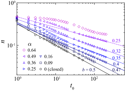
Figure 4: Kink density as a function of $t_{0}$ for various $\alpha$. Solid lines show fitting by a power law $t_{0}^{-b}$ of the rightmost eight data for each $\alpha$. The exponents $b$ thus obtained are shown on the figure. With increasing $\alpha$ from 0, $b$ decreases from $0.5$. The parameters for numerical simulations were chosen as $\Delta t=0.05$, $\chi_{t}=128$, $\chi_{s}=128$, and $\omega_{c}$ = 5.

Figure 4 shows results of our simulation on the kink density $n$ as a function of $t_{0}$. The kink density decays monotonically with $t_{0}$ and obeys the power law $n\sim t_{0}^{-b}$ approximately for large $t_{0}$. The exponent $b$ drawn by fitting the data decreases from 0.5 to around 0.25 with strengthening the system-bath coupling $\alpha$ from 0 up to 0.49, beyond which it is uncertain from our data whether a power law is valid or not.

As mentioned above, the exponents $\nu$ and $z$ are known to be $\nu=z=1$ for $\alpha=0$ by the exact solution of the transverse Ising chain, whereas they are estimated as $\nu\approx 0.63$ and $z\approx 2.0$ for $\alpha>0$ by the QMC simulation Werner et al. (2005). These values predict that $b=0.5$ for $\alpha=0$ and $b\approx 0.28$ for $\alpha>0$. Comparing them to our result, the fact that $b$ is reduced by coupling spins to the bath is shared by the theory and our simulation. However, although the theory predicts a discontinuous change of $b$ from 0.5 to 0.28 by an infinitesimal $\alpha$, our results implies a continuos change of $b$. Moreover, the smallest value of $b$ by our simulation, which is obtained for $\alpha=0.49$, is slightly smaller than 0.28. These discrepancies might be attributed to the range of $t_{0}$. Although our method of simulation is not able to access $t_{0}>200$, the slope of $n$ might be closer to that of $t_{0}^{-0.28}$ if one has much larger $t_{0}$.

Recently, KZM of the transverse Ising chain was studied experimentally using D-Wave’s machines. As mentioned in Sec. I, the physical system in D-Wave’s machine can be regarded as the dissipative transverse Ising model and hence D-Wave’s machine should serve as a quantum simulator of the present model. In fact, it has been reported in ref.Bando et al. (2020) that the kink density decays as $t_{0}^{-b}$ with $b\approx 0.20$ by the device in NASA and $\approx 0.34$ by the low-noise one in Burnaby. We note that the range of $t_{0}$ investigated in these experiments is roughly 4-digit larger than ours. Anyway, the fact that the exponent decreases from 0.5 is common to the experiment, our simulation, and the theory with the QMC simulation. As for the numerical value, the comparison between the experiment and our simulation is difficult, since the strength of the system-bath coupling is unknown for D-Wave’s machines. Nontheless, $b=0.34$ obtained experimentally lies in the range from 0.5 for $\alpha=0$ to $0.25$ for $\alpha=0.49$ by our simulation. Therefore our results are consistent with the experimental result in ref.Bando et al. (2020).

V Conclusion

We investigated KZM of a dissipative transverse Ising chain. First we presented the ground-state phase diagram and confirmed that a quantum phase transition survives even at a finite coupling strength between the spin system and the boson bath. We next showed the energy expectation value of the spin subsystem as a function of time when the spin Hamiltonian varies linearly in time from that of the decoupled spins in the transverse field to that of the Ising chain and when the full system is initialized as the product state of the ground states for spins and bosons. We found that the energy of the spin subsystem relaxes into the value at the ground state of the full system soon and starts to deviate from it at around the quantum critical point. This result implies that KZM takes place in our model. We finally showed the kink density as a function of the time period with which the spin Hamiltonian varies. We observed that the kink density decays as a power law with an exponent $b$ and that $b$ decreases with increasing the system-bath coupling. This fact partly agrees with a theoretical deduction with a QMC result that $b$ changes from 0.5 to 0.28 by an introductin of the system-bath coupling, though the values of $b$ do not always agree. Our results on the kink density, on the other hand, agrees well with an experimental result by D-Wave’s machine. Geting better understanding on $b$ remains to study. To this end, quantum simulators like D-Wave’s machine would be useful.

We used a new numerical algorithm in the present work, which is a combination of the discrete-time path integral representation for the reduced density matrix and iTEBD. This method was for the first time applied to a dissipative quantum many-body model. So far there had been no method to study out-of-equilibrium states of such a model with large system size and without the Born-Markov approximation. The present study will pave the new way to the study of out-of-equilibrium physics in a dissipative quantum many-body system.

The authors thank H. Nishimori and Y. Susa for valuable discussions and Y. Bando, M. Ohzeki, F. J. Gómez-Ruiz, A. del Campo, and D. A. Lidar for collaboration on a related experimental project.

References

- Kibble (1976) T. W. B. Kibble, Journal of Physics A: Mathematical and General 9, 1387 (1976), publisher: IOP Publishing.
- Zurek (1985) W. H. Zurek, Nature 317, 505 (1985).
- Zurek et al. (2005) W. H. Zurek, U. Dorner, and P. Zoller, Phys. Rev. Lett. 95, 105701 (2005), publisher: American Physical Society.
- Polkovnikov (2005) A. Polkovnikov, Phys. Rev. B 72, 161201 (2005), publisher: American Physical Society.
- Polkovnikov et al. (2011) A. Polkovnikov, K. Sengupta, A. Silva, and M. Vengalattore, Rev. Mod. Phys. 83, 863 (2011), publisher: American Physical Society.
- Patané et al. (2008) D. Patané, A. Silva, L. Amico, R. Fazio, and G. E. Santoro, Phys. Rev. Lett. 101, 175701 (2008), publisher: American Physical Society.
- Patané et al. (2009) D. Patané, L. Amico, A. Silva, R. Fazio, and G. E. Santoro, Phys. Rev. B 80, 024302 (2009), publisher: American Physical Society.
- Nalbach et al. (2015) P. Nalbach, S. Vishveshwara, and A. A. Clerk, Phys. Rev. B 92, 014306 (2015), publisher: American Physical Society.
- Dutta et al. (2016) A. Dutta, A. Rahmani, and A. del Campo, Phys. Rev. Lett. 117, 080402 (2016), publisher: American Physical Society.
- Keck et al. (2017) M. Keck, S. Montangero, G. E. Santoro, R. Fazio, and D. Rossini, New Journal of Physics 19, 113029 (2017), publisher: IOP Publishing.
- Arceci et al. (2018) L. Arceci, S. Barbarino, D. Rossini, and G. E. Santoro, Phys. Rev. B 98, 064307 (2018), publisher: American Physical Society.
- Kadowaki and Nishimori (1998) T. Kadowaki and H. Nishimori, Phys. Rev. E 58, 5355 (1998), publisher: American Physical Society.
- Farhi et al. (2001) E. Farhi, J. Goldstone, S. Gutmann, J. Lapan, A. Lundgren, and D. Preda, Science 292, 472 (2001).
- Kato (1950) T. Kato, Journal of the Physical Society of Japan 5, 435 (1950), publisher: The Physical Society of Japan.
- Messiah (1961) A. Messiah, Quantum Mechanics (North Holland, Amsterdam, 1961).
- Sachdev (1999) S. Sachdev, Quantum Phase Transitions (Cambridge University Press, Cambridge, 1999).
- Weiss (2012) U. Weiss, Quantum Dissipative Systems, 4th ed. (World Scientific, Singapore, 2012).
- Suzuki et al. (2019) S. Suzuki, H. Oshiyama, and N. Shibata, Journal of the Physical Society of Japan 88, 061003 (2019), _eprint: https://doi.org/10.7566/JPSJ.88.061003.
- Caldeira and Leggett (1983) A. O. Caldeira and A. J. Leggett, Annals of Physics 149, 374 (1983).
- Leggett et al. (1987) A. J. Leggett, S. Chakravarty, A. T. Dorsey, M. P. A. Fisher, A. Garg, and W. Zwerger, Rev. Mod. Phys. 59, 1 (1987), publisher: American Physical Society.
- Trotter (1959) H. F. Trotter, Proceedings of the American Mathematical Society 10, 545 (1959), publisher: JSTOR.
- Suzuki (1986) M. Suzuki, Journal of Statistical Physics 43, 883 (1986), publisher: Springer.
- Makarov and Makri (1994) D. E. Makarov and N. Makri, Chemical Physics Letters 221, 482 (1994).
- White (2005) S. R. White, Phys. Rev. B 72, 180403 (2005), publisher: American Physical Society.
- White and Feiguin (2004) S. R. White and A. E. Feiguin, Phys. Rev. Lett. 93, 076401 (2004), publisher: American Physical Society.
- Vidal (2007) G. Vidal, Phys. Rev. Lett. 98, 070201 (2007), publisher: American Physical Society.
- Orús and Vidal (2008) R. Orús and G. Vidal, Phys. Rev. B 78, 155117 (2008), publisher: American Physical Society.
- Bulla et al. (2003) R. Bulla, N.-H. Tong, and M. Vojta, Physical review letters 91, 170601 (2003), publisher: APS.
- Werner et al. (2005) P. Werner, K. Völker, M. Troyer, and S. Chakravarty, Phys. Rev. Lett. 94, 047201 (2005), publisher: American Physical Society.
- Strathearn et al. (2018) A. Strathearn, P. Kirton, D. Kilda, J. Keeling, and B. W. Lovett, Nature Communications 9, 3322 (2018).
- Bando et al. (2020) Y. Bando, Y. Susa, H. Oshiyama, N. Shibata, M. Ohzeki, F. J. Gómez-Ruiz, D. A. Lidar, A. del Campo, S. Suzuki, and H. Nishimori, Probing the Universality of Topological Defect Formation in a Quantum Annealer: Kibble-Zurek Mechanism and Beyond (2020) _eprint: 2001.11637.