Emergence of a thermal equilibrium in a subsystem of a pure ground state
by quantum entanglement

Abstract

By numerically exact calculations of spin-1/2 antiferromagnetic Heisenberg models on small clusters up to 24 sites, we demonstrate that quantum entanglement between subsystems $A$ and $B$ in a pure ground state of a whole system $A+B$ can induce thermal equilibrium in subsystem $A$. Here, the whole system is bipartitoned with the entanglement cut that covers the entire volume of subsystem $A$. An effective temperature ${\cal T}_{A}$ of subsystem $A$ induced by quantum entanglement is not a parameter but can be determined from the entanglement von Neumann entropy $\mathcal{S}_{A}$ and the total energy $\mathcal{E}_{A}$ of subsystem $A$ calculated for the ground state of the whole system. We show that temperature ${\cal T}_{A}$ can be derived by minimizing the relative entropy for the reduced density matrix operator of subsystem $A$ and the Gibbs state (i.e., thermodynamic density matrix operator) of subsystem $A$ with respect to the coupling strength between subsystems $A$ and $B$. Temperature ${\cal T}_{A}$ is essentially identical to the thermodynamic temperature, for which the entropy and the internal energy evaluated using the canonical ensemble in statistical mechanics for the isolated subsystem $A$ agree numerically with the entanglement entropy $\mathcal{S}_{A}$ and the total energy $\mathcal{E}_{A}$ of subsystem $A$. Fidelity calculations ascertain that the reduced density matrix operator of subsystem $A$ for the pure but entangled ground state of the whole system $A+B$ matches, within a maximally $1.5\%$ error in the finite size clusters studied, the thermodynamic density matrix operator of subsystem $A$ at temperature ${\cal T}_{A}$, despite that these density-matrix operators are different in general. We also find that temperature ${\cal T}_{A}$ evaluated from the ground state of the whole system depends insignificantly on the system sizes, which is consistent with the fact that the thermodynamic temperature is an intensive quantity. We argue that quantum fluctuation in an entangled pure state can mimic thermal fluctuation in a subsystem. We also provide two simple but nontrivial analytical examples of free bosons and free fermions for which the two density-matrix operators are exactly the same if the effective temperature ${\cal T}_{A}$ is adopted. We furthermore discuss implications and possible applications of our finding.

I Introduction

How thermal equilibrium arises in a pure quantum state has been an attractive subject of study in statistical mechanics [1]. This is often addressed by examining how the time average of an expectation value of observable for a pure quantum state after relaxation dynamics approaches an ensemble average of the corresponding observable [2, 3, 4, 5, 6, 7, 8]. Recently, the eigenstate-thermalization hypothesis (ETH) [9, 10, 11, 12, 13] is widely exploited as a useful concept for investigating the thermalization in isolated quantum systems. The ETH hypothesizes that expectation values of few-body observables with respect to energy eigenstates in a given energy shell behave as microcanonical expectation values of the corresponding energy shell (see Ref. [14] for details). However, not all quantum states satisfy the ETH [15] and systems that do not follow the ETH can be systematically constructed [16, 17].

The typicality [18, 19, 20, 21], which characterizes thermal equilibrium rather than thermalization, is also considered as an important concept for foundation of statistical mechanics. The typicality states that for almost every pure state randomly sampled from the Hilbert space, a single measurement of observable converges to the corresponding statistical expectation value with probability close to $1$ (see Ref. [22] for detail). Based on the typicality, it has been shown that statistical mechanics can be formulated in terms of the thermal pure quantum (TPQ) states [23, 24, 25], rather than conventional mixed states. Note that construction of a TPQ state involves multiplications of Hamiltonian in non-unitary forms.

Another key ingredient for foundation of statistical mechanics from a quantum-mechanical point of view is the entanglement [18]. Consider a normalized pure state $|\Psi\rangle$ in a Hilbert space $\mathcal{H}$, and divide the Hilbert space into two, $\mathcal{H}=\mathcal{H}_{A}\otimes\mathcal{H}_{B}$. The reduced density matrix operator $\hat{\rho}_{A}$ on $\mathcal{H}_{A}$ is defined as $\hat{\rho}_{A}={\rm Tr}_{B}[|\Psi\rangle\langle\Psi|]$, where ${\rm Tr}_{B}[\cdot]$ denotes the trace over $\mathcal{H}_{B}$. Since $\hat{\rho}_{A}$ is Hermitian $(\hat{\rho}_{A}^{\dagger}=\hat{\rho}_{A})$, positive semidefinite $(\hat{\rho}_{A}\geqslant 0)$, and normalized $({\rm Tr}_{A}[\hat{\rho}_{A}]=1)$, it has the form of $\hat{\rho}_{A}=\exp(-\hat{\mathcal{I}}_{A})$ with $\hat{\mathcal{I}}_{A}$ being a Hermitian operator on $\mathcal{H}_{A}$. $\hat{\mathcal{I}}_{A}$ is referred to as entanglement Hamiltonian and its spectrum [26] is the entanglement spectrum. Following Li and Haldane [27], one can consider $\hat{\rho}_{A}$ as the Gibbs state of “Hamiltonian” $\hat{\mathcal{I}}_{A}$ at “temperature” $T=1$.

The entanglement Hamiltonian or the entanglement spectrum has been studied for various quantum states, such as the quantum Hall state [26, 28], Tomonaga-Luttinger liquids [29, 30], the ground state of the Heisenberg model [31, 32], the ground state of the Hubbard model [33], the ground states in different phases of magnetic impurity models [34, 35], the valence-bond solid states [36], and a time-evolved random-product states of the quantum Ising model [37], either by numerical or analytical techniques. Remarkably, it has been shown for the quantum Hall state that the entanglement Hamiltonian is proportional to the Hamiltonian at the boundary [28]. Also, near the limit of maximal entanglement under certain conditions, a proportionality between the entanglement Hamiltonian and the Hamiltonian of a subsystem has been found [38]. Moreover, for a wide class of spin models in one-dimensional (1D) and two-dimensional (2D) lattices, it has been shown that an entanglement temperature, which is defined by means of a field-theoretical approach, varies spatially and decreases inversely proportional to the distance from the entanglement cut that divides the system into two half spaces  [39, 40, 41]. These results imply a possibility to find a physical interpretation for the entanglement Hamiltonian, at least, in some cases. Moreover, a recent cold-atom experiment [42] has shown that through a unitary evolution of a pure state, thermalization occurs on a local scale, and has pointed out the importance of the entanglement entropy for thermalization.

Such formal similarities between a reduced density matrix operator and a Gibbs state may naturally raise a question as to whether a thermal equilibrium state in statistical mechanics can emerge from a pure quantum state described by quantum mechanics. To this end, disentangling the “temperature” from the entanglement Hamiltonian in a reduced density matrix operator is a crucial step. In this paper, we address this issue by numerically analyzing the ground states of spin-1/2 antiferromagnetic Heisenberg models in two coupled 1D chains (i.e., two-leg ladder) and in two coupled 2D square and triangular lattices (i.e., bilayer lattice) (see Fig. 1 and Fig. 2). Under a bipartitioning of the whole system into subsystems with an entanglement cut that covers the entire volume of the subsystem, our numerical calculations strongly support that a thermal equilibrium can emerge in a partitioned subsystem of a pure ground state with the temperature that is not a parameter but is determined by the entanglement von Neumann entropy and the total energy of the subsystem. This is further ascertained numerically by the fidelity calculation of the reduced density matrix operator and the Gibbs state. We also provide two simple but nontrivial examples, relevant to the Unruh effect or a two-mode squeezed state in quantum optics and a BCS-type superconducting state, to support this statement analytically.

The rest of the paper is organized as follows. In Sec. II, we introduce the Heisenberg Hamiltonian and describe the setup of bipartitioning the system. We also briefly review the reduced density matrix operator for a subsystem of a ground state and the Gibbs state in the canonical ensemble. In Sec. III, we show the numerically exact results revealing that the entanglement von Neumann entropy and the total energy of the subsystem are almost identical with the thermodynamic entropy and the internal energy of the isolated subsystem, respectively, provided that a certain form of the effective temperature is introduced. Moreover, the fidelity between the reduced density matrix operator and the Gibbs state is examined. In Sec. IV, we consider two examples that can be solved analytically, for which the reduced density matrix operator is exactly the same as the Gibbs state, thus supporting the numerical finding. In Sec. V, we further discuss the implication of the emergent thermal equilibrium in a partitioned subsystem of a pure ground state. In Sec. VI, we conclude the paper with remarks on possible application and extension of the present finding. Additional discussions on the effective temperature, the relative entropy, and the thermofield-double state are given in Appendices A,  B, and  C, respectively. Throughout the paper, we set $\hbar=1$ and $k_{B}=1$.

II Model and Formalism

II.1 Model and bipartitioning

We consider the spin-1/2 antiferromagnetic Heisenberg model described by the following Hamiltonian:

$$\hat{H} = \sum_{\langle i,j\rangle}J_{ij}\ \hat{\boldsymbol{S}}_{i}\cdot\hat{\boldsymbol{S}}_{j}$$ (1)

where $\langle i,j\rangle$ runs over all pairs of nearest-neighbor sites $i$ and $j$ in two coupled 1D chains (i.e., two-leg ladder) or in two coupled 2D square or triangular lattices (i.e., bilayer lattice). $\boldsymbol{\hat{S}}_{i}$ is the spin-$1/2$ operator located at the $i$th site and the nearest-neighbor spins are connected with the exchange interaction $J_{ij}=J_{A}$, $J_{B}$, or $\lambda$ (see Fig. 1). We denote by $N$ the number of spins and thus the dimension of the total Hilbert space $\mathcal{H}$ is $D=\dim\mathcal{H}=2^{N}$. We consider the case where the exchange interactions are antiferromagnetic ($J_{ij}>0$).

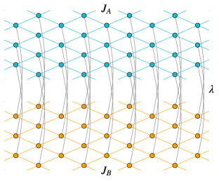
Figure 1: Schematic figure of the whole system $A+B$ consisting of subsystems $A$ (upper layer indicated by cyan) and $B$ (lower layer indicated by orange), which are coupled via the exchange interaction $\lambda$, indicated by curved black lines. The exchange interactions between spins in subsystems $A$ and $B$ are $J_{A}$ and $J_{B}$, respectively. In this study, we consider the bipartitioning of the whole system into subsystems with the entanglement cut that covers the entire volume of subsystem $A$.

To study the entanglement in the ground state of $\hat{H}$, we bipartition the Hilbert space $\mathcal{H}$ of the whole system into those of subsystems $A$ and $B$ as $\mathcal{H}=\mathcal{H}_{A}\otimes\mathcal{H}_{B}$. Accordingly, the Hamiltonian $\hat{H}$ can be written as

$$\hat{H}(\lambda)=\hat{H}_{A}\otimes\hat{I}_{B}+\hat{I}_{A}\otimes\hat{H}_{B}+\hat{V}_{AB}(\lambda),$$ (2)

where

$$\hat{H}_{A}=J_{A}\sum_{\langle i,j\rangle\in A}\hat{\boldsymbol{S}}_{i}\cdot\hat{\boldsymbol{S}}_{j},$$ (3)

$$\hat{H}_{B}=J_{B}\sum_{\langle i,j\rangle\in B}\hat{\boldsymbol{S}}_{i}\cdot\hat{\boldsymbol{S}}_{j},$$ (4)

$$\hat{V}_{AB}(\lambda)=\lambda\sum_{\langle i,j\rangle,i\in A,j\in B}\hat{\boldsymbol{S}}_{i}\cdot\hat{\boldsymbol{S}}_{j},$$ (5)

and $\hat{I}_{A\,(B)}$ is the identity operator on $\mathcal{H}_{A\,(B)}$ (see Fig. 1). $\hat{H}_{A\,(B)}$ is the Hamiltonian of subsystem $A$ $(B)$ and $\hat{V}_{AB}(\lambda)$ describes the exchange interaction between subsystems $A$ and $B$. The subsystem $B$ considered here is essentially a copy of the subsystem $A$ except that its interaction strength $J_{B}$ may differ from $J_{A}$. We denote by $N_{A\,(B)}$ the number of spins in subsystem $A$ $(B)$ and thus the dimension of the Hilbert space for subsystem $A$ $(B)$ is $D_{A\,(B)}=\dim\mathcal{H}_{A\,(B)}=2^{N_{A\,(B)}}$. Note that $N=N_{A}+N_{B}$ and $D=D_{A}D_{B}$. The exchange interaction $\lambda$ controls the entanglement between subsystems $A$ and $B$. As shown schematically in Fig. 1, the whole system is bipartitioned into two subsystems $A$ and $B$ with the entanglement cut that covers the entire volume of subsystem $A$.

Let $|\Psi_{0}(\lambda)\rangle$ be the normalized ground state of $\hat{H}(\lambda)$. Note that the $\lambda$ dependency of $\hat{H}$ and $|\Psi_{0}\rangle$ is explicitly denoted since we consider the entanglement between subsystems $A$ and $B$ in the ground state $|\Psi_{0}(\lambda)\rangle$ with varying $\lambda$. Although the ground state should depend on the exchange interactions as $|\Psi_{0}\rangle=|\Psi_{0}(J_{B}/J_{A},\lambda/J_{A})\rangle$, here we simply assume the $J_{A}$ and $J_{B}$ dependence of these quantities.

Four remarks are in order. In our setup, (i) we do not assume any finite temperature in the subsystem $A$ or $B$, (ii) the volume $N_{B}$ of subsystem $B$ is not necessarily sufficiently larger than the volume $N_{A}$ of subsystem $A$ (and vice versa), (iii) the coupling term $\hat{V}_{AB}(\lambda)$ between subsystems $A$ and $B$ is not necessarily small as compared to $\hat{H}_{A}$ and $\hat{H}_{B}$, and (iv) a pure state of the whole system $A+B$ is always chosen as its ground state $|\Psi_{0}(\lambda)\rangle$, and thus any stochastic sampling of pure states from $\mathcal{H}$ does not apply. Remarks (i)-(iii) imply that the role of subsystem $B$ is not the heat bath for subsystem $A$, unlike in the conventional statistical mechanics. Remark (iv) implies that our approach do not make use of the typicality argument.

II.2 Entanglement entropy and energy of subsystem $A$

The ground state can be expanded as

$$|\Psi_{0}(\lambda)\rangle=\sum_{i=1}^{D}c_{i}(\lambda)|i\rangle=\sum_{i=1}^{D_{A}}\sum_{j=1}^{D_{B}}c_{i,j}(\lambda)|{i}\rangle_{A}|{j}\rangle_{B},$$ (6)

where $\{|i\rangle\}_{i=1}^{D}$ is the orthonormal basis set in $\mathcal{H}$, and $\{|i\rangle_{A\,(B)}\}_{i=1}^{D_{A\,(B)}}$ is the orthonormal basis set in $\mathcal{H}_{A\,(B)}$. The coefficients $\{c_{i}(\lambda)\}_{i=1}^{D}$ are rewritten as $\{c_{i,j}(\lambda)\}_{i=1,j=1}^{D_{A},D_{B}}$ simply by using the labels $i$ and $j$ for subsystems $A$ and $B$. The reduced density matrix operator $\hat{\rho}_{A}^{\rm red}$ of subsystem $A$ is now given as

$$\hat{\rho}_{A}^{\rm red}(\lambda) ={\rm Tr}_{B}\left[|\Psi_{0}(\lambda)\rangle\langle\Psi_{0}(\lambda)|\right]$$

$$=\sum_{k=1}^{D_{B}}{{}_{B}}\langle k|\Psi_{0}(\lambda)\rangle\langle\Psi_{0}(\lambda)|k\rangle_{B}$$

$$=\sum_{i=1}^{D_{A}}\sum_{j=1}^{D_{A}}\rho^{\rm red}_{A,ij}(\lambda){|i\rangle_{A}}{{}_{A}}\langle j|,$$ (7)

where the reduced density matrix

$$\rho^{\rm red}_{A,ij}(\lambda)\equiv\sum_{k=1}^{D_{B}}c_{i,k}(\lambda)c_{j,k}^{*}(\lambda)$$ (8)

is introduced. With a $D_{A}\times D_{B}$ matrix $\boldsymbol{c}(\lambda)$ defined as $[\boldsymbol{c}(\lambda)]_{ij}=c_{i,j}(\lambda)$, the reduced density matrix can be written in a matrix form as $\boldsymbol{\rho}^{\rm red}_{A}(\lambda)=\boldsymbol{c}(\lambda)\boldsymbol{c}(\lambda)^{\dagger}$. The reduced density matrix $\boldsymbol{\rho}^{\rm red}_{A}(\lambda)$ is Hermitian and positive semidefinite, and satisfies ${\rm Tr}[\boldsymbol{\rho}^{\rm red}_{A}(\lambda)]=\langle\Psi_{0}(\lambda)|\Psi_{0}(\lambda)\rangle=1$ [43]. The positive semidefiniteness of $\boldsymbol{\rho}^{\rm red}_{A}(\lambda)$ follows from the fact that $\boldsymbol{\rho}^{\rm red}_{A}(\lambda)$ is a Gram matrix as apparently noticed in Eq. (8).

The entanglement entropy $\mathcal{S}_{A}(\lambda)$ of subsystem $A$ is here defined as the von Neumann entropy of the reduced density matrix operator,

$$\mathcal{S}_{A}(\lambda)\equiv{\rm Tr}_{A}\left[\hat{\rho}^{\rm red}_{A}(\lambda)\hat{\mathcal{I}}^{\rm red}_{A}(\lambda)\right]=-{\rm Tr}_{A}\left[\hat{\rho}^{\rm red}_{A}(\lambda)\ln{\hat{\rho}^{\rm red}_{A}(\lambda)}\right]$$ (9)

with $\hat{\mathcal{I}}_{A}^{\rm red}(\lambda)=-\ln\hat{\rho}^{\rm red}_{A}(\lambda)$ being the entanglement Hamiltonian. The entanglement entropy satisfies $0\leqslant\mathcal{S}_{A}\leqslant\ln D_{A}$, where the lower bound is achieved when $\hat{\rho}_{A}^{\rm red}$ is a pure state and the upper bound is obtained when $\hat{\rho}_{A}^{\rm red}$ is the maximally mixed state. The energy $\mathcal{E}_{A}(\lambda)$ of subsystem $A$ is calculated as

$$\mathcal{E}_{A}(\lambda)\equiv{\rm Tr}_{A}\left[\hat{\rho}^{\rm red}_{A}(\lambda)\hat{H}_{A}\right]=\langle\Psi_{0}(\lambda)|\hat{H}_{A}\otimes\hat{I}_{B}|\Psi_{0}(\lambda)\rangle.$$ (10)

Note that these quantities are defined using the ground-state wavefunction $|\Psi_{0}(\lambda)\rangle$ of the whole system $\hat{H}(\lambda)$.

II.3 Canonical ensemble of subsystem $A$

Let us consider the canonical ensemble in statistical mechanics for the isolated subsystem $A$ without subsystem $B$. In the canonical ensemble, the heat bath with temperature $T$ is assumed and the average of an observable $\hat{\mathcal{O}}$ in subsystem $A$ is given as

$$\left\langle\hat{\mathcal{O}}\right\rangle_{\beta}^{\rm can}\equiv{\rm Tr}_{A}\left[\hat{\rho}_{A}^{\rm can}(\beta)\hat{\mathcal{O}}\right],$$ (11)

where

$$\hat{\rho}_{A}^{\rm can}(\beta)\equiv\frac{{\rm e}^{-\beta\hat{H}_{A}}}{Z_{A}(\beta)}$$ (12)

is the Gibbs state, i.e., thermodynamic density matrix operator, $\beta=1/T$ is the inverse temperature, and $Z_{A}(\beta)={\rm Tr}_{A}\left[{\rm e}^{-\beta\hat{H}_{A}}\right]$ is the partition function. The entropy $S_{A}(\beta)$ and the internal energy $E_{A}(\beta)$ are given, respectively, as

$$S_{A}(\beta) =\left\langle\mathcal{I}^{\rm can}_{A}(\beta)\right\rangle_{\beta}^{\rm can}=-{\rm Tr}_{A}\left[\hat{\rho}_{A}^{\rm can}(\beta)\ln\hat{\rho}_{A}^{\rm can}(\beta)\right]$$ (13)

and

$$E_{A}(\beta) =\left\langle\hat{H}_{A}\right\rangle_{\beta}^{\rm can}={\rm Tr}_{A}\left[\hat{\rho}_{A}^{\rm can}(\beta)\hat{H}_{A}\right]$$ (14)

with $\hat{\mathcal{I}}_{A}^{\rm can}(\beta)=-\ln\hat{\rho}_{A}^{\rm can}(\beta)$.

III Numerical Results

By numerically analyzing the Heisenberg models described above, we now examine the emergence of a thermal equilibrium in the partitioned subsystem $A$ by quantum entanglement. First, we briefly review two limiting cases when $\lambda=0$ (i.e., zero entanglement limit) and $\lambda=\infty$ (i.e., maximal entanglement limit). Next, we show numerical results for general values of $\lambda$, which support the emergent thermal equilibrium, provided that the temperature is appropriately introduced.

III.1 Zero entanglement and zero-temperature limit

When $\lambda=0$, there exists no entanglement between subsystems $A$ and $B$ and any eigenstate of $\hat{H}(\lambda=0)$ is separable under the bipartioning of the system considered here. In particular, the ground state $|\Psi_{0}(\lambda=0)\rangle$ is the product state of the ground states $|\psi_{0}^{A}\rangle$ and $|\psi_{0}^{B}\rangle$ of subsystems $A$ and $B$, respectively, i.e., $|\Psi_{0}(\lambda=0)\rangle=|\psi_{0}^{A}\rangle|\psi_{0}^{B}\rangle$. Thus, the subsystem $A$ is a pure state and the reduced density matrix operator of subsystem $A$ is

$$\hat{\rho}_{A}^{\rm red}(\lambda=0)=|\psi^{A}_{0}\rangle\langle\psi^{A}_{0}|$$ (15)

with the entanglement von Neumann entry of subsystem $A$

$$\mathcal{S}_{A}(\lambda=0)=0,$$ (16)

which is the lower bound of $\mathcal{S}_{A}$. The thermodynamic density matrix operator in the zero-temperature limit is apparently identical with the reduced density matrix operator at $\lambda=0$, i.e.,

$$\hat{\rho}_{A}^{\rm can}(\beta=\infty)=\hat{\rho}_{A}^{\rm red}(\lambda=0),$$ (17)

and the thermodynamic entropy is $S_{A}(\beta=\infty)=0$.

III.2 Maximal entanglement and infinite-temperature limit

When $\lambda=\infty$, the total Hamiltonian $\hat{H}(\lambda)$ is dominated by $\hat{V}_{AB}(\lambda)$ and the corresponding ground state $|\Psi_{0}(\lambda=\infty)\rangle$ is a singlet-pair product state, i.e., the direct product of the spin singlet states formed by two neighboring spins, each locating in subsystems $A$ and $B$. Thus, $|\Psi_{0}(\infty)\rangle$ has the maximal entanglement between subsystems $A$ and $B$. After tracing out subsystem $B$, the subsystem $A$ is described by the maximally mixed state (see a similar argument in Ref. [44]) and the reduced density matrix operator of subsystem $A$ is

$$\hat{\rho}_{A}^{\rm red}(\lambda=\infty)=\frac{1}{D_{A}}\hat{I}_{A}$$ (18)

with the entanglement von Neumann entropy of subsystem $A$

$$\mathcal{S}_{A}(\lambda=\infty)=\ln{D_{A}}=N_{A}\ln 2,$$ (19)

which is the upper bound of $\mathcal{S}_{A}$. The thermodynamic density matrix operator in the infinite-temperature limit is identical with the reduced density matrix operator at $\lambda=\infty$, i.e.,

$$\hat{\rho}_{A}^{\rm can}(\beta=0)=\hat{\rho}_{A}^{\rm red}(\lambda=\infty),$$ (20)

and the thermodynamic entropy is $S_{A}(\beta=0)=N_{A}\ln 2$.

III.3 General values of $\lambda$ and $\beta$

We calculate the ground state $|\Psi_{0}(\lambda)\rangle$ of $\hat{H}(\lambda)$ by the Lanczos method, and evaluate $\mathcal{S}_{A}(\lambda)$ and $\mathcal{E}_{A}(\lambda)$ of subsystem $A$, accordingly to the formalism described in Sec. II.2. To examine how these entanglement-induced quantities of the ground state $|\Psi_{0}(\lambda)\rangle$ can be related to the thermodynamic quantities of the subsystem, we also calculate $S_{A}(\beta)$ and $E_{A}(\beta)$ of the isolated subsystem $A$ as a function of the inverse temperature $\beta=1/T$ by numerically diagonalizing the Hamiltonian $\hat{H}_{A}$ (see Sec. II.3). The finite-size systems used for these calculations are shown in Fig. 2. We should emphasize that the ground state $|\Psi_{0}(\lambda)\rangle$ of $\hat{H}(\lambda)$ is spin singlet (i.e., total spin and thus the $z$ component of the total spin being both zero) and the total momentum of $|\Psi_{0}(\lambda)\rangle$ is zero, while the canonical ensemble described in Sec. II.3 averages over all eigenstates of $\hat{H}_{A}$ in all spin and momentum symmetry sectors.

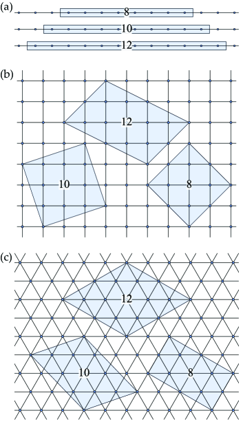
Figure 2: Finite-size clusters of $N_{A}=8,10,$ and $12$ on (a) the 1D chain, (b) the 2D square lattice, and (c) the 2D triangular lattice used for the calculations. Periodic-boundary conditions are applied for all clusters. The figures show only the subsystem $A$, which couples to the subsystem $B$ with $N_{B}=N_{A}$ when the ground state of the whole system ${\hat{H}}(\lambda)={\hat{H}}_{A}+{\hat{H}}_{B}+{\hat{V}}_{AB}(\lambda)$ is calculated (see Fig. 1).

Figure 3 shows the $\lambda$ dependence of $\mathcal{S}_{A}(\lambda)$ and $\mathcal{E}_{A}(\lambda)$ with different values of $J_{B}/J_{A}$. For comparison, the $T$ dependence of $S_{A}(\beta)$ and $E_{A}(\beta)$ is also shown. It is clearly observed that $\mathcal{S}_{A}(\lambda)$ and $\mathcal{E}_{A}(\lambda)$ increase monotonically with $\lambda$. Moreover, as discussed in Sec. III.1 and Sec. III.2, the ranges of the entanglement von Neumann entropy $\mathcal{S}_{A}(\lambda)$ and the thermodynamic entropy $S_{A}(\beta)$ with varying $\lambda$ and $T$, respectively, as well as those of $\mathcal{E}_{A}(\lambda)$ and $E_{A}(\beta)$, agree with each other.

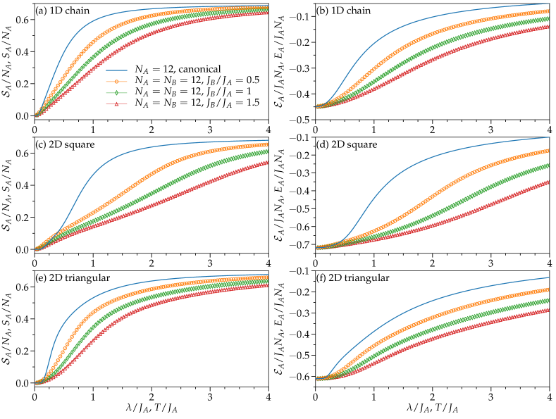
Figure 3: (a,c,e) The entanglement von Neumann entropy per site $\mathcal{S}_{A}(\lambda)/N_{A}$ of subsystem $A$ as a function of $\lambda/J_{A}$ for several values of $J_{B}$ (symbols) and the thermodynamic entropy per site $S_{A}(\beta)/N_{A}$ of the isolated subsystem $A$ as a function of temperature $T$ (solid line). (b,d,f) The energy per site $\mathcal{E}_{A}(\lambda)/N_{A}$ of subsystem $A$ as a function of $\lambda/J_{A}$ for several values of $J_{B}$ (symbols) and the internal energy per site $E_{A}(\beta)/N_{A}$ of the isolated subsystem $A$ as a function of temperature $T$ (solid line). In (a) and (b), $\mathcal{S}_{A}(\lambda)$ and $\mathcal{E}_{A}(\lambda)$ are calculated for the two coupled 1D chains (i.e., two-leg ladder) with $N_{A}=N_{B}=12$, and $S_{A}(\beta)$ and $E_{A}(\beta)$ are calculated for the 1D chain with $N_{A}=12$. In (c) and (d), $\mathcal{S}_{A}(\lambda)$ and $\mathcal{E}_{A}(\lambda)$ are calculated for the two coupled 2D square lattices (i.e., bilayer square lattice) with $N_{A}=N_{B}=12$, and $S_{A}(\beta)$ and $E_{A}(\beta)$ are calculated for the 2D square lattice with $N_{A}=12$. In (e) and (f), $\mathcal{S}_{A}(\lambda)$ and $\mathcal{E}_{A}(\lambda)$ are calculated for the two coupled 2D triangular lattices (i.e., bilayer triangular lattice) with $N_{A}=N_{B}=12$, and $S_{A}(\beta)$ and $E_{A}(\beta)$ are calculated for the 2D triangular lattice with $N_{A}=12$.

Figure 4 shows the same quantities $\mathcal{S}_{A}(\lambda)$ and $\mathcal{E}_{A}(\lambda)$ but as a function of an effective temperature defined as $\mathcal{T}_{A}(\lambda)=1/\mathcal{B}_{A}(\lambda)$ with

$$\mathcal{B}_{A}(\lambda)=\lim_{\Delta\lambda\to 0}\frac{\mathcal{S}_{A}(\lambda+\Delta\lambda)-\mathcal{S}_{A}(\lambda)}{\mathcal{E}_{A}(\lambda+\Delta\lambda)-\mathcal{E}_{A}(\lambda)}=\frac{\partial_{\lambda}\mathcal{S}_{A}(\lambda)}{\partial_{\lambda}\mathcal{E}_{A}(\lambda)}.$$ (21)

In the numerical calculations, we evaluate $\mathcal{B}_{A}(\lambda)$ for $\lambda\geqslant\Delta\lambda$ by a central finite difference $\mathcal{B}_{A}(\lambda)\approx(\mathcal{S}_{A}(\lambda+\Delta\lambda)-\mathcal{S}_{A}(\lambda-\Delta\lambda))/(\mathcal{E}_{A}(\lambda+\Delta\lambda)-\mathcal{E}_{A}(\lambda-\Delta\lambda))$ with $\Delta\lambda/J_{A}=0.02$. For comparison, the $T$ dependence of $S_{A}(\beta)$ and $E_{A}(\beta)$ of the canonical ensemble is also shown in Fig. 4. Remarkably, for each lattice structure, $\mathcal{S}_{A}(\lambda)$ for all $J_{B}/J_{A}$ values are on a universal curve [Figs. 4(a), 4(c), and 4(e)]. Moreover, such a universal curve essentially coincides with the temperature dependence of the thermodynamic entropy $S_{A}(\beta)$ for the corresponding lattice. The same is also found in the energy $\mathcal{E}_{A}(\lambda)$ and the internal energy $E_{A}(\beta)$, as shown in Figs. 4(b), 4(d), and 4(f). Note that a lack of data points around the limit of $\mathcal{T}_{A}(\lambda)=0$ in Fig. 4 is due to the finite-difference scheme employed for evaluating $\mathcal{B}_{A}(\lambda)=\mathcal{T}_{A}(\lambda)^{-1}$ in Eq. (21). If smaller $\Delta\lambda$ is chosen, one may find more data points around this limit.

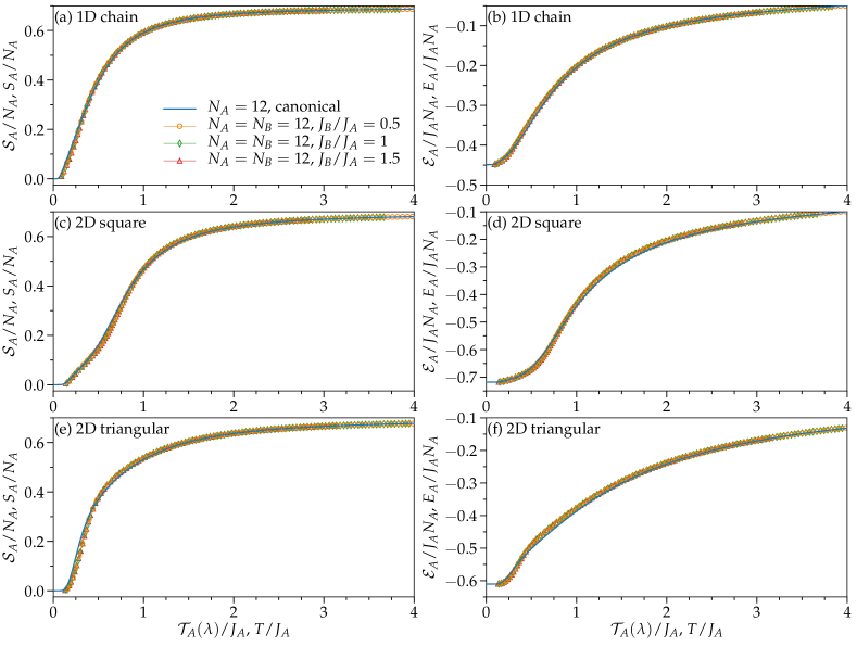
Figure 4: Same as Fig. 3 but $\mathcal{S}_{A}(\lambda)$ and $\mathcal{E}_{A}(\lambda)$ are now plotted as a function of $\mathcal{T}_{A}(\lambda)$.

Figure 5 shows the effective temperature $\mathcal{T}_{A}(\lambda)$ as a function of $\lambda$. While the dependence of $\mathcal{T}_{A}(\lambda)$ on $\lambda$ is nontrivial, $\mathcal{T}_{A}(\lambda)$ increases monotonically with $\lambda$. We can also notice that the increase of $\mathcal{T}_{A}(\lambda)$ is more significant for smaller $J_{B}/J_{A}$. Furthermore, we find that $\mathcal{T}_{A}(\lambda)$ depends insignificantly on the system size, as expected for an analog to the thermodynamic temperature, which is an intensive quantity. A relatively large deviation of $\mathcal{T}_{A}(\lambda)$ for the smallest cluster ($N_{A}=N_{B}=8$), observed in Fig. 5(c) for the triangular lattice at low effective temperatures $\mathcal{T}_{A}(\lambda)/J_{A}\lesssim 2$, might be due to the strong finite-size effect.

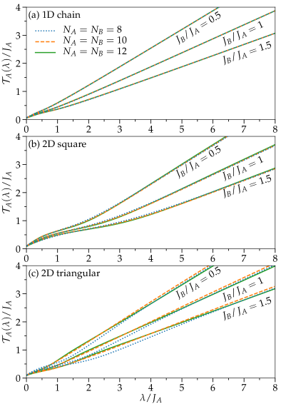
Figure 5: The effective temperature $\mathcal{T}_{A}(\lambda)$ as a function of $\lambda$ calculated for (a) the two coupled 1D chains (i.e., two-leg ladder), (b) the two coupled 2D square lattices (i.e., bilayer square lattice), and (c) the two coupled 2D triangular lattices (i.e., bilayer triangular lattice) with $N_{A}=N_{B}=8,10,$ and $12$. The results for $J_{B}/J_{A}=0.5$, 1, and 1.5 are shown (from top to bottom in each panel).

We note that the form of Eq. (21) for the effective temperature is apparently analogous to the definition of the inverse temperature in thermodynamics [45], except that there is the microscopic parameter $\lambda$, through which $\mathcal{S}_{A}(\lambda)$ and $\mathcal{E}_{A}(\lambda)$ are mediated. Indeed, Eq. (21) can be derived by minimizing the relative entropy for the reduced density matrix operator and the thermodynamic density matrix operator with respect to $\lambda$. Here, the relative entropy for density matrix operators $\hat{\rho}_{0}$ and $\hat{\rho}_{1}$ is defined as $D(\hat{\rho}_{1}|\hat{\rho}_{0})={\rm Tr}\left[\hat{\rho}_{1}\ln\hat{\rho}_{1}\right]-{\rm Tr}\left[\hat{\rho}_{1}\ln\hat{\rho}_{0}\right]$ with the trace taken over the Hilbert space on which $\hat{\rho}_{0}$ and $\hat{\rho}_{1}$ are defined (also see Appendix A). Substituting $\hat{\rho}_{0}=\hat{\rho}_{A}^{\rm can}(\beta)$ and $\hat{\rho}_{1}=\hat{\rho}_{A}^{\rm red}(\lambda)$ into $D(\hat{\rho}_{1}|\hat{\rho}_{0})$, we obtain that

$$D[\hat{\rho}_{A}^{\rm red}(\lambda)|\hat{\rho}_{A}^{\rm can}(\beta)]=-\mathcal{S}_{A}(\lambda)+\beta\mathcal{E}_{A}(\lambda)+\ln{Z_{A}(\beta)}.$$ (22)

It is interesting to notice that there is the “cross term” in the right hand side of Eq. (22) between quantities representing the quantum entanglement, i.e., the ground state energy $\mathcal{E}_{A}(\lambda)$ of subsystem $A$, and thermodynamics, i.e., the inverse temperature $\beta$. The minimization of $D[\hat{\rho}_{A}^{\rm red}(\lambda)|\hat{\rho}_{A}^{\rm can}(\beta)]$ with respect to $\lambda$, i.e., $\frac{\partial D[\hat{\rho}_{A}^{\rm red}(\lambda)|\hat{\rho}_{A}^{\rm can}(\beta)]}{\partial\lambda}=0$, yields

$$\beta=\frac{\partial_{\lambda}\mathcal{S}_{A}(\lambda)}{\partial_{\lambda}\mathcal{E}_{A}(\lambda)}=\mathcal{B}_{A}(\lambda).$$ (23)

Therefore, when we consider $\lambda$ as a variable, $\beta$ should be determined as in Eq. (21). We can also minimize $D[\hat{\rho}_{A}^{\rm red}(\lambda)|\hat{\rho}_{A}^{\rm can}(\beta)]$ with respect to $\beta$, which yields

$$\mathcal{E}_{A}(\lambda)=E_{A}(\beta),$$ (24)

suggesting that when we consider $\beta$ as a variable, $\lambda$ should be determined so as to satisfy Eq. (24). Although we do not adopt the latter, it turns out that Eq. (24) is almost perfectly satisfied in our numerical calculations shown in Fig. 4, if $\beta$ is determined by Eq. (21). It should be noted that the relative entropy is not symmetric, i.e., $D(\hat{\rho}_{1}|\hat{\rho}_{0})\not=D(\hat{\rho}_{0}|\hat{\rho}_{1})$ for $\hat{\rho}_{0}\not=\hat{\rho}_{1}$, and the minimization of $D[\hat{\rho}_{A}^{\rm can}(\beta)|\hat{\rho}_{A}^{\rm red}(\lambda)]$ with respect to either $\lambda$ or $\beta$ does not yield Eq. (23). Further discussions on $\mathcal{B}_{A}(\lambda)$ in the form of Eq. (21) are given in Sec. V.1.

Excellent collapse of different quantities, $\mathcal{S}_{A}(\lambda)\simeq S_{A}(\mathcal{B}_{A}(\lambda))$ and $\mathcal{E}_{A}(\lambda)\simeq E_{A}(\mathcal{B}_{A}(\lambda))$, implies that the relation

$$\hat{\rho}_{A}^{\rm red}(\lambda)\simeq\hat{\rho}_{A}^{\rm can}(\mathcal{B}_{A}(\lambda))$$ (25)

holds between the reduced density matrix operator $\hat{\rho}_{A}^{\rm red}(\lambda)$ and the thermodynamic density matrix operator $\hat{\rho}_{A}^{\rm can}(\beta)$, independently of the detail of the subsystem $B$ whose degrees of freedom are traced out, as schematically shown in Fig. 6. To quantify the similarity between these two density matrix operators, we calculate the fidelity $F$ of density matrix operators $\hat{\rho}$ and $\hat{\sigma}$ on $\mathcal{H}_{A}$ defined as

$$F(\hat{\rho},\hat{\sigma})=\left({\rm Tr}_{A}\sqrt{\sqrt{\hat{\rho}}\hat{\sigma}\sqrt{\hat{\rho}}}\right)^{2}$$ (26)

for $\hat{\rho}=\hat{\rho}_{A}^{\rm can}(\mathcal{B}_{A}(\lambda))$ and $\hat{\sigma}=\hat{\rho}_{A}^{\rm red}(\lambda)$. Note that the fidelity satisfies $F(\hat{\rho},\hat{\sigma})=1$ if and only if $\hat{\rho}=\hat{\sigma}$, and generally $0\leqslant F(\hat{\rho},\hat{\sigma})\leqslant 1$  [46, 47].

Figure 7 shows the fidelity per site, $F^{\frac{1}{N_{A}}}$, calculated for the three different lattice structures with $J_{B}/J_{A}=1$. As expected from the discussion in Sec. III.1 and Sec. III.2, the fidelity tends to $1$ in the limits of $\mathcal{T}_{A}(\lambda)\to 0$ and $\mathcal{T}_{A}(\lambda)\to\infty$. More interestingly, the fidelity per site is kept large (at least larger than $0.985$) even at intermediate $\mathcal{T}_{A}(\lambda)$, verifying Eq. (25) quantitatively (see insets of Fig. 7). However, except for the triangular lattice, the fidelity per site tends to become smaller with increasing the system size. Obviously, calculations with larger clusters are desirable to further examine the finite-size effects, but currently are not feasible due to the exponentially large computational cost. We note that the fidelity with $J_{B}/J_{A}=0.5$ and $J_{B}/J_{A}=1.5$ does not significantly differ from that with $J_{B}/J_{A}=1$.

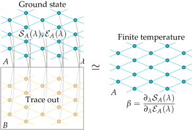
Figure 6: Schematic figure featuring that a thermal equilibrium at temperature $T=1/\beta$ (right) emerges in a bipartitioned subsystem of a pure ground state by quantum entanglement controlled with $\lambda$ (left). This implies that the quantum fluctuation mimics the thermal fluctuation.

While the fidelity deviates from 1 most significantly in the intermediate temperatures, the differences in $\mathcal{S}_{A}(\lambda)$ and $S_{A}(\mathcal{B}_{A}(\lambda))$ and in $\mathcal{E}_{A}(\lambda)$ and $E_{A}(\mathcal{B}_{A}(\lambda))$ are not much visible, at least in the scale shown in Fig. 4. To examine how the deviation of the fidelity from 1 might reflect on microscopic observables, here we calculate the spin correlation function in the subsystem $A$

$$C_{ij}(\hat{\rho})={\rm Tr}_{A}\left[\hat{\rho}\hat{S}_{i}^{z}\hat{S}_{j}^{z}\right]$$ (27)

for $\hat{\rho}=\hat{\rho}_{A}^{\rm red}(\lambda)$ and $\hat{\rho}=\hat{\rho}_{A}^{\rm can}(\mathcal{B}_{A}(\lambda))$, where $\hat{S}_{i}^{z}$ is the $z$ component of spin $\boldsymbol{\hat{S}}_{i}$ at site $i\in A$. Note that the nearest-neighbor spin correlation function is essentially equivalent to the energy $\mathcal{E}_{A}(\lambda)/N_{A}$ or $E_{A}(\mathcal{B}_{A}(\lambda))/N_{A}$ because the Hamiltonian $\hat{H}_{A}$ includes only the nearest-neighbor interactions.

Figure 8 shows the difference of the spin correlation function

$$\delta C_{ij}(\lambda)=C_{ij}(\hat{\rho}_{A}^{\rm can}(\mathcal{B}_{A}(\lambda)))-C_{ij}(\hat{\rho}_{A}^{\rm red}(\lambda))$$ (28)

as a function of $\mathcal{T}_{A}(\lambda)$ with $J_{B}/J_{A}=1$. Here we focus on the 1D systems with $N_{A}=8,10,$ and $12$ to find a systematic dependence on the system size. Due to the periodic-boundary conditions, $\delta C_{ij}$ for the 1D systems depends only on the spatial distance $|i-j|$ between sites $i$ and $j$. It is found that the difference of the next-nearest neighbor and longer-range ($|i-j|\geqslant 2$) spin correlation functions is pronounced in the temperature range where the fidelity exhibits a dip. On the other hand, the difference in the nearest-neighbor ($|i-j|=1$) correlation function is less significant, as expected from the energy calculations. It is also found that, the maximum of the absolute difference of the spin correlation function, $\max|\delta C_{ij}(\lambda)|$, among different temperatures remains almost unchanged for $|i-j|=1$ and even tends to decrease for $|i-j|\geqslant 2$ with increasing the size $N_{A}$, in spite of the decrease of the fidelity with increasing $N_{A}$ (see Fig. 9). These results suggest that the difference between the two density matrix operators $\hat{\rho}_{A}^{\rm red}(\lambda)$ and $\hat{\rho}_{A}^{\rm can}(\mathcal{B}_{A}(\lambda))$ in the intermediate temperatures can cause a rather prominent signature in microscopic quantities such as the longer-range spin correlation functions that do not contribute to the energy.

Although the strong finite-size effect do not allow us to perform a systematic analysis for the 2D square and triangular lattices, we have also found that, in the temperature range where the fidelity deviates from 1, the spin correlation functions beyond the nearest-neighbor distance tend to differ most in the 2D systems.

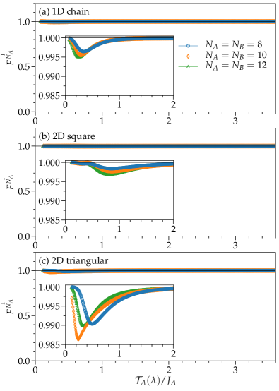
Figure 7: The fidelity per site $F(\hat{\rho},\hat{\sigma})^{\frac{1}{N_{A}}}$ for $\hat{\rho}=\hat{\rho}_{A}^{\rm can}(\mathcal{B}_{A}(\lambda))$ and $\hat{\sigma}=\hat{\rho}_{A}^{\rm red}(\lambda)$ as a function of the effective temperature $\mathcal{T}_{A}(\lambda)$ calculated for (a) the two coupled 1D chains (i.e., two-leg ladder), (b) the two coupled 2D square lattices (i.e., bilayer square lattice), and (c) the two coupled 2D triangular lattices (i.e., bilayer triangular lattice) with $N_{A}=N_{B}=8,10,$ and $12$. The insets show enlarged plots for $\mathcal{T}_{A}(\lambda)/J_{A}\leqslant 2$ and $F^{\frac{1}{N_{A}}}\simeq 1$. $J_{B}/J_{A}=1$ is assumed.

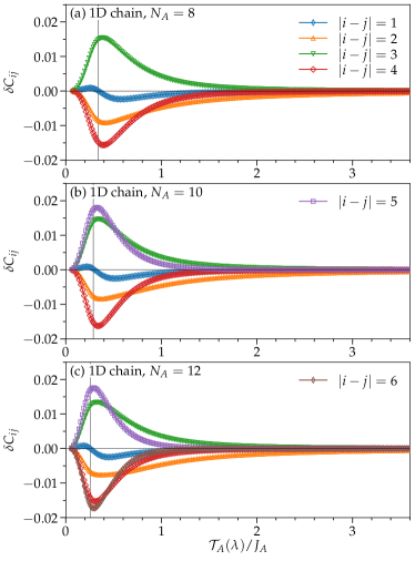
Figure 8: The difference of the spin correlation function $\delta C_{ij}$ for various values of the spatial distance $|i-j|$ as a function of the effective temperature $\mathcal{T}_{A}(\lambda)$. The results are obtained for the 1D chain with (a) $N_{A}=8$, (b) $N_{A}=10$, and (c) $N_{A}=12$. The vertical line indicates the temperature where the fidelity $F$ deviates most from 1 in Fig. 7(a).

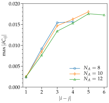
Figure 9: The maximum of the absolute difference of the spin correlation functions, $\max|\delta C_{ij}|$, among different temperatures shown in Fig. 8 as a function of the spatial distance $|i-j|$ for the 1D chain with $N_{A}=$8, 10, and 12. Due to the translational symmetry, only the results for $1\leqslant|i-j|\leqslant N_{A}/2$ are shown.

IV Two analytical examples

To support the numerical finding in Sec. III, here we consider two examples, free bosons and free fermions under pairing field, which can be solved analytically, and show that the reduced density matrix operator of a partitioned subsystem of a ground state is identical to the thermodynamic density matrix operator, provided that the effective temperature is properly introduced as in Eq. (21).

IV.1 Bosons under pairing field

First we analyze the entanglement between free bosons under pairing field by considering the Hamiltonian of the form in Eq. (2) with

$$\hat{H}_{A}=\omega_{A}\left(\hat{a}^{\dagger}\hat{a}+\frac{1}{2}\right),$$ (29)

$$\hat{H}_{B}=\omega_{B}\left(\hat{b}^{\dagger}\hat{b}+\frac{1}{2}\right),$$ (30)

and

$$\hat{V}_{AB}(\lambda)=\lambda\left(\hat{a}\hat{b}+\hat{b}^{\dagger}\hat{a}^{\dagger}\right),$$ (31)

where $\hat{a}$ and $\hat{b}$ are boson annihilation operators on $\mathcal{H}_{A}$ and $\mathcal{H}_{B}$, respectively. The operators satisfy the commutation relations $[\hat{a},\hat{a}^{\dagger}]=1$, $[\hat{b},\hat{b}^{\dagger}]=1$, $[\hat{a},\hat{b}^{\dagger}]=0$, and $[\hat{a},\hat{b}]=0$. We assume that $\omega_{A}>0$, $\omega_{B}>0$, and $|\lambda|<(\omega_{A}+\omega_{B})/2$. More precise restrictions on the parameters are discussed after Eq. (39).

By introducing new bosonic operators $\hat{\alpha}$ and $\hat{\beta}$ via a Bogoliubov transformation as

$$\begin{bmatrix}\hat{\alpha}\\ \hat{\beta}^{\dagger}\end{bmatrix}=\begin{bmatrix}\cosh\theta&\sinh\theta\\ \sinh\theta&\cosh\theta\end{bmatrix}\begin{bmatrix}\hat{a}\\ \hat{b}^{\dagger}\end{bmatrix}$$ (32)

with $\theta$ satisfying that

$$\lambda=\omega\tanh(2\theta)$$ (33)

and

$$\omega=\frac{\omega_{A}+\omega_{B}}{2},$$ (34)

the Hamiltonian $\hat{H}(\lambda)$ can be diagonalized as

$$\hat{H}(\lambda)=\Omega_{\alpha}\hat{\alpha}^{\dagger}\hat{\alpha}+\Omega_{\beta}\hat{\beta}^{\dagger}\hat{\beta}+E_{0},$$ (35)

where

$$\Omega_{\alpha}=\frac{\omega_{A}\cosh^{2}{\theta}-\omega_{B}\sinh^{2}{\theta}}{\cosh^{2}{\theta}+\sinh^{2}{\theta}},$$ (36)

$$\Omega_{\beta}=\frac{\omega_{B}\cosh^{2}{\theta}-\omega_{A}\sinh^{2}{\theta}}{\cosh^{2}{\theta}+\sinh^{2}{\theta}},$$ (37)

and

$$E_{0}=\frac{\omega}{\cosh^{2}{\theta}+\sinh^{2}{\theta}}=\frac{\Omega_{\alpha}+\Omega_{\beta}}{2}.$$ (38)

Let us assume that

$$\Omega_{\alpha}>0\text{\quad and \quad}\Omega_{\beta}>0.$$ (39)

These inequalities are satisfied for any $\theta$ if $\omega_{A}=\omega_{B}$. However, if $\omega_{A}\not=\omega_{B}$, these inequalities are satisfied only in a limited range of $\theta$. For example, if $\omega_{B}/\omega_{A}<1$, $\Omega_{\alpha}>0$ is satisfied for any $\theta$ but $\Omega_{\beta}>0$ is satisfied only if $\tanh^{2}{\theta}<\omega_{B}/\omega_{A}<1$. A similar condition can be found for $\omega_{A}/\omega_{B}<1$. Below we only consider the parameter region that satisfies the inequalities in Eq. (39).

Since $\Omega_{\alpha}>0$ and $\Omega_{\beta}>0$, the ground state $|\Psi_{0}(\lambda)\rangle$ of $\hat{H}(\lambda)$ should be a vacuum state of bosons $\hat{\alpha}$ and $\hat{\beta}$ satisfying $\hat{\alpha}|\Psi_{0}(\lambda)\rangle=0$ and $\hat{\beta}|\Psi_{0}(\lambda)\rangle=0$. Using the vacuum states $|0\rangle_{A}$ and $|0\rangle_{B}$ in $\mathcal{H}_{A}$ and $\mathcal{H}_{B}$, respectively satisfying $\hat{a}|0\rangle_{A}=0$ and $\hat{b}|0\rangle_{B}=0$, the ground state can be given explicitly as

$$|\Psi_{0}(\lambda)\rangle =\frac{1}{\cosh{\theta}}{\rm e}^{-(\tanh{\theta})\hat{a}^{\dagger}\hat{b}^{\dagger}}|0\rangle_{A}|0\rangle_{B}$$

$$=\frac{1}{\cosh{\theta}}\sum_{n=0}^{\infty}(-\tanh{\theta})^{n}|n\rangle_{A}|n\rangle_{B},$$ (40)

with $|n\rangle_{A}=(n!)^{-1/2}(\hat{a}^{\dagger})^{n}|0\rangle_{A}$ and $|n\rangle_{B}=(n!)^{-1/2}(\hat{b}^{\dagger})^{n}|0\rangle_{B}$. The entangled state of the form in Eq. (40) has several applications including the Unruh effect [48, 49] and a two-mode squeezed state in quantum optics [50].

By tracing out the degrees of freedom in $\mathcal{H}_{B}$ from the ground-state density matrix operator $|\Psi_{0}\rangle\langle\Psi_{0}|$, we obtain the reduced density matrix operator of subsystem $A$:

$$\hat{\rho}_{A}^{\rm red}(\lambda)=\frac{1}{\cosh^{2}{\theta}}\sum_{n=0}^{\infty}(\tanh^{2}{\theta})^{n}|n\rangle_{A}{{}_{A}\langle n|}.$$ (41)

On the other hand, by noticing $\hat{H}_{A}|n\rangle_{A}=\omega_{A}(n+\frac{1}{2})|n\rangle_{A}$, the thermodynamic density matrix operator of the isolated subsystem $A$ is given by

$$\hat{\rho}_{A}^{\rm can}(\beta) = (1-{\rm e}^{-\beta\omega_{A}})\sum_{n=0}^{\infty}{\rm e}^{-\beta\omega_{A}n}|n\rangle_{A}{{}_{A}\langle n|}$$ (42)

$$= ({\rm e}^{\beta\omega_{A}/2}-{\rm e}^{-\beta\omega_{A}/2})\sum_{n=0}^{\infty}{\rm e}^{-\beta\omega_{A}\left(n+\frac{1}{2}\right)}|n\rangle_{A}{{}_{A}\langle n|}.$$ (43)

By comparing Eq. (41) with Eq. (42), it is found that $\hat{\rho}_{A}^{\rm red}(\lambda)$ is exactly the same as $\hat{\rho}_{A}^{\rm can}(\beta)$ when $\beta=\beta_{A}^{\star}$ with

$$\beta_{A}^{\star} =-\frac{1}{\omega_{A}}\ln{\tanh^{2}{\theta}}$$ (44)

$$=-\frac{1}{\omega_{A}}\ln\left[\frac{\omega}{\lambda}\pm\sqrt{\left(\frac{\omega}{\lambda}\right)^{2}-1}\right]^{2},$$ (45)

where $+$ ($-$) sign is taken for $\theta>0$ ($\theta<0$). Figures 10(a) and 10(b) show $\theta$ and $\lambda$ dependence of $\beta_{A}^{\star}$ and $T_{A}^{\star}=1/\beta_{A}^{\star}$, respectively. We can furthermore find that the entanglement Hamiltonian $\hat{\mathcal{I}}^{\rm red}_{A}=-\ln\hat{\rho}_{A}^{\rm red}$ is proportional to $\hat{H}_{A}$ with coefficient $\beta_{A}^{\star}$:

$$\hat{\mathcal{I}}^{\rm red}_{A}=\beta_{A}^{\star}\hat{H}_{A}+\frac{1}{2}\ln Z_{A}^{2},$$ (46)

where $Z_{A}^{2}=\cosh^{2}{\theta}\sinh^{2}{\theta}=\left({\rm e}^{\beta_{A}^{\star}\omega_{A}/2}-{\rm e}^{-\beta_{A}^{\star}\omega_{A}/2}\right)^{-2}$ and the spectral representation of the number operator $\hat{a}^{\dagger}\hat{a}=\sum_{n=0}^{\infty}n|n\rangle_{A}{{}_{A}}\langle n|$ is used. Next, we shall show that the inverse temperature $\beta^{\star}_{A}$ given in Eq. (44) is the same as the effective inverse temperature $\mathcal{B}_{A}(\lambda)=\partial_{\lambda}{\mathcal{S}_{A}}/\partial_{\lambda}{\mathcal{E}_{A}}$ introduced in Eq. (21).

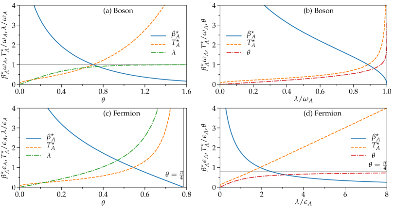
Figure 10: $\beta_{A}^{\star}$, $T_{A}^{\star}\,(=1/\beta_{A}^{\star})$, and $\lambda$ as a function of $\theta$ for (a) the bosonic system with $\omega_{A}=\omega_{B}$ and (c) the fermionic system with $\epsilon_{A}=\epsilon_{B}$. $\beta_{A}^{\star}$, $T_{A}^{\star}\,(=1/\beta_{A}^{\star})$, and $\theta$ as a function of $\lambda$ for (b) the bosonic system with $\omega_{A}=\omega_{B}$ and (d) the fermionic system with $\epsilon_{A}=\epsilon_{B}$. The horizontal line in (a) indicates the asymptote of $\lim_{\theta\to\infty}\lambda(\theta)/\omega_{A}=1$, the vertical line in (c) indicates $\theta=\pi/4$, and the horizontal line in (d) indicates the asymptote of $\lim_{\lambda\to\infty}\theta(\lambda)=\pi/4$.

The effective inverse temperature $\mathcal{B}_{A}(\lambda)$ is evaluated from the entanglement von Neumann entropy $\mathcal{S}_{A}(\lambda)$ and the energy $\mathcal{E}_{A}(\lambda)$ of subsystem $A$ for the ground state $|\Psi_{0}(\lambda)\rangle$. Equation (41) implies that $\hat{\rho}_{A}^{\rm red}(\lambda)$ contains the eigenstate $|n\rangle_{A}$ of $\hat{H}_{A}$ with the probability

$$p_{n}=\frac{(\tanh^{2}\theta)^{n}}{\cosh^{2}\theta}.$$ (47)

Therefore, the entanglement von Neumann entropy $\mathcal{S}_{A}(\lambda)$ is calculated as

$$\mathcal{S}_{A}(\lambda) =-{\rm Tr}_{A}\left[\hat{\rho}_{A}^{\rm red}(\lambda)\ln\hat{\rho}_{A}^{\rm red}(\lambda)\right]$$

$$=-\sum_{n=0}^{\infty}p_{n}\ln p_{n}$$

$$=(\cosh^{2}\theta)\ln{\cosh^{2}{\theta}}-(\sinh^{2}\theta)\ln{\sinh^{2}{\theta}},$$ (48)

where $\sum_{n=0}^{\infty}nx^{n}=x/(1-x)^{2}$ for $|x|<1$ is used in the last equality. Similarly, the energy $\mathcal{E}_{A}(\lambda)$ is calculated as

$$\mathcal{E}_{A}(\lambda) ={\rm Tr}_{A}\left[\hat{\rho}_{A}^{\rm red}(\lambda)\hat{H}_{A}\right]$$

$$=\omega_{A}\sum_{n=0}^{\infty}p_{n}\left(n+\frac{1}{2}\right)$$

$$=\omega_{A}\left(\sinh^{2}{\theta}+\frac{1}{2}\right),$$ (49)

where $\sum_{n=0}^{\infty}p_{n}=1$ is used. We thus find that $\partial_{\theta}\mathcal{S}_{A}=-(2\cosh\theta\sinh\theta)\ln\tanh^{2}\theta$ and $\partial_{\theta}\mathcal{E}_{A}=2\omega_{A}\cosh\theta\sinh\theta$. Therefore, the effective inverse temperature $\mathcal{B}_{A}(\lambda)$ is calculated as

$$\mathcal{B}_{A}(\lambda)=\frac{\partial_{\lambda}\theta\ \partial_{\theta}\mathcal{S}_{A}}{\partial_{\lambda}\theta\ \partial_{\theta}\mathcal{E}_{A}}=-\frac{1}{\omega_{A}}\ln\tanh^{2}{\theta}=\beta_{A}^{\star}.$$ (50)

From Eqs. (41)–(44) and (50), we can conclude that the relation

$$\hat{\rho}_{A}^{\rm can}(\mathcal{B}_{A}(\lambda))=\hat{\rho}_{A}^{\rm red}(\lambda)$$ (51)

holds exactly and thus is no longer a conjecture in this case.

We note that the relation in Eq. (50) can also be derived by directly calculating $\partial\mathcal{S}_{A}/\partial\mathcal{E}_{A}$. Namely, it follows from Eq. (49) that $\sinh^{2}{\theta}=\frac{\mathcal{E}_{A}}{\omega_{A}}-\frac{1}{2}$ and $\cosh^{2}{\theta}=\frac{\mathcal{E}_{A}}{\omega_{A}}+\frac{1}{2}$. Therefore, $\mathcal{S}_{A}$ can be expressed in terms of $\mathcal{E}_{A}$ as

$$\mathcal{S}_{A}=\left(\frac{\mathcal{E}_{A}}{\omega_{A}}+\frac{1}{2}\right)\ln\left(\frac{\mathcal{E}_{A}}{\omega_{A}}+\frac{1}{2}\right)-\left(\frac{\mathcal{E}_{A}}{\omega_{A}}-\frac{1}{2}\right)\ln\left(\frac{\mathcal{E}_{A}}{\omega_{A}}-\frac{1}{2}\right),$$ (52)

and thus one can readily show that

$$\frac{\partial\mathcal{S}_{A}}{\partial\mathcal{E}_{A}}=\beta_{A}^{\star}.$$ (53)

To confirm more specifically the correspondence between the two density matrix operators in Eq. (51), let us rewrite the entanglement von Neumann entropy $\mathcal{S}_{A}$ and the energy $\mathcal{E}_{A}$ in terms of $\beta_{A}^{\star}$, instead of $\theta$. It follows from Eq. (44) that

$$\tanh^{2}{\theta}={\rm e}^{-\beta_{A}^{\star}\omega_{A}},$$ (54)

$$\cosh^{2}\theta=1+n_{\beta_{A}^{\star}}(\omega_{A}),$$ (55)

and

$$\sinh^{2}\theta=n_{\beta_{A}^{\star}}(\omega_{A}),$$ (56)

where

$$n_{\beta_{A}^{\star}}(\omega_{A})=\frac{1}{{\rm e}^{\beta_{A}^{\star}\omega_{A}}-1}$$ (57)

is the Bose-Einstein distribution function at inverse temperature $\beta_{A}^{\star}$. Substituting Eqs. (55) and (56) into Eqs. (48) and (49) yields that

$$\mathcal{S}_{A} =(1+n_{\beta_{A}^{\star}})\ln(1+n_{\beta_{A}^{\star}})-n_{\beta_{A}^{\star}}\ln n_{\beta_{A}^{\star}}$$ (58)

and

$$\mathcal{E}_{A} =\omega_{A}\left(n_{\beta_{A}^{\star}}+\frac{1}{2}\right),$$ (59)

which are familiar forms of the thermodynamic entropy and the internal energy of free bosons, respectively. One can also readily find that the positive square root $Z_{A}=\left({\rm e}^{\beta^{\star}_{A}\omega_{A}/2}-{\rm e}^{-\beta^{\star}_{A}\omega_{A}/2}\right)^{-1}>0$ of $Z_{A}^{2}$ gives the corresponding partition function, i.e., $Z_{A}={\rm Tr}_{A}\left[{\rm e}^{-\beta^{\star}_{A}\hat{H}_{A}}\right]$.

By doing the same analysis for subsystem $B$, one can find the relation between the effective temperatures $\mathcal{T}_{A}(\lambda)=\mathcal{B}_{A}^{-1}(\lambda)$ and $\mathcal{T}_{B}(\lambda)=\mathcal{B}_{B}^{-1}(\lambda)$ as

$$\mathcal{T}_{A}(\lambda)/\omega_{A}=\mathcal{T}_{B}(\lambda)/\omega_{B}.$$ (60)

Finally, we note that all these analyses given above are based on the ground state in Eq. (40) under the conditions in Eq. (39). One can readily show that if $\omega_{A}\not=\omega_{B}$, the maximum of the effective temperature is bounded. For example, when $\omega_{B}/\omega_{A}<1$, $\tanh^{2}{\theta}<\omega_{B}/\omega_{A}$ should be satisfied in order to satisfy the conditions in Eq. (39). This implies that $\ln{(\omega_{A}/\omega_{B})}<\beta_{A}^{\star}\omega_{A}<\infty$, or equivalently $0<T_{A}^{\star}/\omega_{A}<1/\ln{(\omega_{A}/\omega_{B})}$.

IV.2 Fermions under pairing field

Next we analyze the entanglement between free fermions under pairing field by considering the Hamiltonian of the form in Eq. (2) with

$$\hat{H}_{A}=\epsilon_{A}\left(\hat{a}^{\dagger}\hat{a}-\frac{1}{2}\right),$$ (61)

$$\hat{H}_{B}=\epsilon_{B}\left(\hat{b}^{\dagger}\hat{b}-\frac{1}{2}\right),$$ (62)

and

$$\hat{V}_{AB}(\lambda)=\lambda\left(\hat{a}\hat{b}+\hat{b}^{\dagger}\hat{a}^{\dagger}\right),$$ (63)

where $\hat{a}$ and $\hat{b}$ are fermion annihilation operators on $\mathcal{H}_{A}$ and $\mathcal{H}_{B}$, respectively. The subtraction of $1/2$ in Eqs. (61) and (62) is made simply to find a formal similarity with the bosonic case. The operators satisfy the anticommutation relations $\{\hat{a},\hat{a}^{\dagger}\}=1$, $\{\hat{b},\hat{b}^{\dagger}\}=1$, $\{\hat{a},\hat{b}^{\dagger}\}=0$, and $\{\hat{a},\hat{b}\}=0$. Here we assume that $\epsilon_{A}>0$ and $\epsilon_{B}>0$. An interpretation of this assumption is, for example, that we consider the coupling between two fermion particles (holes) added above (below) the Fermi sea, with the energies $\epsilon_{A}$ and $\epsilon_{B}$ measured from the Fermi level. More precise restrictions on the parameters are discussed after Eq. (71).

By introducing new fermionic operators $\hat{\alpha}$ and $\hat{\beta}$ via a Bogoliubov transformation as

$$\begin{bmatrix}\hat{\alpha}\\ \hat{\beta}^{\dagger}\end{bmatrix}=\begin{bmatrix}\cos\theta&-\sin\theta\\ \sin\theta&\cos\theta\end{bmatrix}\begin{bmatrix}\hat{a}\\ \hat{b}^{\dagger}\end{bmatrix}$$ (64)

with $\theta$ satisfying that

$$\lambda =\epsilon\tan(2\theta)$$ (65)

and

$$\epsilon =\frac{\epsilon_{A}+\epsilon_{B}}{2},$$ (66)

the Hamiltonian $\hat{H}(\lambda)$ can be diagonalized as

$$\hat{H}(\lambda)=\xi_{\alpha}\hat{\alpha}^{\dagger}\hat{\alpha}+\xi_{\beta}\hat{\beta}^{\dagger}\hat{\beta}+E_{0},$$ (67)

where

$$\xi_{\alpha}=\epsilon_{A}\cos^{2}{\theta}-\epsilon_{B}\sin^{2}{\theta},$$ (68)

$$\xi_{\beta}=\epsilon_{B}\cos^{2}{\theta}-\epsilon_{A}\sin^{2}{\theta},$$ (69)

and

$$E_{0}=-\epsilon(\cos^{2}{\theta}-\sin^{2}{\theta})=-\frac{\xi_{\alpha}+\xi_{\beta}}{2}.$$ (70)

Similarly to the bosonic case, we assume that

$$\xi_{\alpha}>0\text{\quad and \quad}\xi_{\beta}>0.$$ (71)

If $\epsilon_{A}=\epsilon_{B}$, these inequalities are satisfied for $-\frac{\pi}{4}<\theta<\frac{\pi}{4}$, implying that $-\infty<\lambda<\infty$. However, if $\epsilon_{A}\not=\epsilon_{B}$, the range of $\theta$ and hence $\lambda$ allowed is more restricted. For example, if $\epsilon_{B}/\epsilon_{A}<1$, $\xi_{\alpha}>0$ is satisfied for any $\theta$ but $\xi_{\beta}>0$ is satisfied only if $\tan^{2}{\theta}<\epsilon_{B}/\epsilon_{A}<1$. A similar condition can be found for $\epsilon_{A}/\epsilon_{B}<1$. Below we only consider the parameter region that satisfies the inequalities in Eq. (71).

Since $\xi_{\alpha}>0$ and $\xi_{\beta}>0$, the ground state $|\Psi_{0}(\lambda)\rangle$ of $\hat{H}(\lambda)$ should be a vacuum state of fermions $\hat{\alpha}$ and $\hat{\beta}$ satisfying $\hat{\alpha}|\Psi_{0}(\lambda)\rangle=0$ and $\hat{\beta}|\Psi_{0}(\lambda)\rangle=0$. Using the vacuum states $|0\rangle_{A}$ and $|0\rangle_{B}$ in $\mathcal{H}_{A}$ and $\mathcal{H}_{B}$, respectively satisfying $\hat{a}|0\rangle_{A}=0$ and $\hat{b}|0\rangle_{B}=0$, the ground state can be given explicitly as

$$|\Psi_{0}(\lambda)\rangle =\cos{\theta}{\rm e}^{(\tan\theta)\hat{a}^{\dagger}\hat{b}^{\dagger}}|0\rangle_{A}|0\rangle_{B}$$

$$=\cos{\theta}\sum_{n=0}^{1}(\tan{\theta})^{n}|n\rangle_{A}|n\rangle_{B},$$ (72)

with $|n\rangle_{A}=(\hat{a}^{\dagger})^{n}|0\rangle_{A}$ and $|n\rangle_{B}=(\hat{b}^{\dagger})^{n}|0\rangle_{B}$. The multi-mode-generalization of the entangled state of the form in Eq. (72) is the Bardeen-Cooper-Schrieffer (BCS) wave function [51].

By tracing out the degrees of freedom in $\mathcal{H}_{B}$ from the ground-state density matrix operator $|\Psi_{0}\rangle\langle\Psi_{0}|$, we obtain the reduced density matrix operator of subsystem $A$:

$$\hat{\rho}_{A}^{\rm red}(\lambda)=\cos^{2}{\theta}\sum_{n=0}^{1}(\tan^{2}{\theta})^{n}|n\rangle_{A}{{}_{A}\langle n|}.$$ (73)

On the other hand, by noticing $\hat{H}_{A}|n\rangle_{A}=\epsilon_{A}(n-\frac{1}{2})|n\rangle_{A}$, the thermodynamic density matrix operator of subsystem $A$ is given by

$$\hat{\rho}_{A}^{\rm can}(\beta) = \frac{1}{1+{\rm e}^{-\beta\epsilon_{A}}}\sum_{n=0}^{1}{\rm e}^{-\beta\epsilon_{A}n}|n\rangle_{A}{{}_{A}\langle n|}$$ (74)

$$= \frac{1}{{\rm e}^{\beta\epsilon_{A}/2}+{\rm e}^{-\beta\epsilon_{A}/2}}\sum_{n=0}^{1}{\rm e}^{-\beta\epsilon_{A}\left(n-\frac{1}{2}\right)}|n\rangle_{A}{{}_{A}\langle n|}.$$ (75)

By comparing Eq. (73) with Eq. (74), it is found that $\hat{\rho}_{A}^{\rm red}(\lambda)$ is exactly the same as $\hat{\rho}_{A}^{\rm can}(\beta)$ when $\beta=\beta_{A}^{\star}$ with

$$\beta_{A}^{\star} =-\frac{1}{\epsilon_{A}}\ln{\tan^{2}{\theta}}$$ (76)

$$=-\frac{1}{\epsilon_{A}}\ln\left[-\frac{\epsilon}{\lambda}\pm\sqrt{\left(\frac{\epsilon}{\lambda}\right)^{2}+1}\right]^{2},$$ (77)

where $+$ ($-$) sign is taken for $\theta>0$ ($\theta<0$). Figures 10(c) and 10(d) show $\theta$ and $\lambda$ dependence of $\beta_{A}^{\star}$ and $T_{A}^{\star}=1/\beta_{A}^{\star}$, respectively. We can furthermore find that the entanglement Hamiltonian $\hat{\mathcal{I}}^{\rm red}_{A}=-\ln\hat{\rho}_{A}^{\rm red}$ is proportional to $\hat{H}_{A}$ with coefficient $\beta_{A}^{\star}$:

$$\hat{\mathcal{I}}_{A}^{\rm red}=\beta_{A}^{\star}\hat{H}_{A}+\frac{1}{2}\ln Z_{A}^{2},$$ (78)

where $Z_{A}^{2}=1/\cos^{2}{\theta}\sin^{2}{\theta}=\left({\rm e}^{\beta^{\star}_{A}\epsilon_{A}/2}+{\rm e}^{-\beta^{\star}_{A}\epsilon_{A}/2}\right)^{2}$ and the spectral representation of the number operator $\hat{a}^{\dagger}\hat{a}=\sum_{n=0}^{1}n|n\rangle_{A}{{}_{A}}\langle n|$ is used. Next, we shall show that the inverse temperature $\beta^{\star}_{A}$ given in Eq. (76) is the same as the effective inverse temperature $\mathcal{B}_{A}(\lambda)=\partial_{\lambda}{\mathcal{S}_{A}}/\partial_{\lambda}{\mathcal{E}_{A}}$ introduced in Eq. (21).

The effective inverse temperature $\mathcal{B}_{A}$ is evaluated from the entanglement von Neumann entropy $\mathcal{S}_{A}(\lambda)$ and the energy $\mathcal{E}_{A}(\lambda)$ of subsystem $A$ for the ground state $|\Psi_{0}(\lambda)\rangle$. Equation (73) implies that $\hat{\rho}_{A}^{\rm red}(\lambda)$ contains the eigenstate $|n\rangle_{A}$ of $\hat{H}_{A}$ with the probability

$$p_{n}=\cos^{2}\theta(\tan^{2}\theta)^{n},$$ (79)

or more explicitly $p_{0}=\cos^{2}\theta$ and $p_{1}=\sin^{2}\theta$. Therefore, the entanglement von Neumann entropy $\mathcal{S}_{A}(\lambda)$ is calculated as

$$\mathcal{S}_{A}(\lambda) =-{\rm Tr}_{A}\left[\hat{\rho}_{A}^{\rm red}(\lambda)\ln\hat{\rho}_{A}^{\rm red}(\lambda)\right]$$

$$=-\sum_{n=0}^{1}p_{n}\ln p_{n}$$

$$=-(\cos^{2}\theta)\ln{\cos^{2}{\theta}}-(\sin^{2}\theta)\ln{\sin^{2}{\theta}},$$ (80)

Similarly, the energy $\mathcal{E}_{A}(\lambda)$ is calculated as

$$\mathcal{E}_{A}(\lambda) ={\rm Tr}_{A}\left[\hat{\rho}_{A}^{\rm red}(\lambda)\hat{H}_{A}\right]$$

$$=\epsilon_{A}\sum_{n=0}^{1}p_{n}\left(n-\frac{1}{2}\right)$$

$$=\epsilon_{A}\left(\sin^{2}{\theta}-\frac{1}{2}\right).$$ (81)

We thus find that $\partial_{\theta}\mathcal{S}_{A}=(2\cos\theta\sin\theta)\ln\tan^{2}\theta$ and $\partial_{\theta}\mathcal{E}_{A}=-2\epsilon_{A}\cos\theta\sin\theta$. Therefore, the effective inverse temperature $\mathcal{B}_{A}(\lambda)$ is calculated as

$$\mathcal{B}_{A}(\lambda)=\frac{\partial_{\lambda}\theta\ \partial_{\theta}\mathcal{S}_{A}}{\partial_{\lambda}\theta\ \partial_{\theta}\mathcal{E}_{A}}=-\frac{1}{\epsilon_{A}}\ln\tan^{2}{\theta}=\beta_{A}^{\star}.$$ (82)

From Eqs (73)–(76) and (82), we can conclude that the relation

$$\hat{\rho}_{A}^{\rm can}(\mathcal{B}_{A}(\lambda))=\hat{\rho}_{A}^{\rm red}(\lambda)$$ (83)

holds exactly and thus is no longer a conjecture in this case.

We note that the relation in Eq. (82) can be derived also by directly calculating $\partial\mathcal{S}_{A}/\partial\mathcal{E}_{A}$. Namely, it follows from Eq. (81) that $\sin^{2}{\theta}=\frac{1}{2}+\frac{\mathcal{E}_{A}}{\epsilon_{A}}$ and $\cos^{2}{\theta}=\frac{1}{2}-\frac{\mathcal{E}_{A}}{\epsilon_{A}}$. Therefore, $\mathcal{S}_{A}$ can be expressed in terms of $\mathcal{E}_{A}$ as

$$\mathcal{S}_{A}=-\left(\frac{1}{2}-\frac{\mathcal{E}_{A}}{\epsilon_{A}}\right)\ln\left(\frac{1}{2}-\frac{\mathcal{E}_{A}}{\epsilon_{A}}\right)-\left(\frac{1}{2}+\frac{\mathcal{E}_{A}}{\epsilon_{A}}\right)\ln\left(\frac{1}{2}+\frac{\mathcal{E}_{A}}{\epsilon_{A}}\right),$$ (84)

and thus one can readily show that

$$\frac{\partial\mathcal{S}_{A}}{\partial\mathcal{E}_{A}}=\beta_{A}^{\star}.$$ (85)

To confirm more specifically the correspondence between the two density matrix operators in Eq. (83), let us rewrite the entanglement von Neumann entropy $\mathcal{S}_{A}$ and the energy $\mathcal{E}_{A}$ in terms of $\beta_{A}^{\star}$, instead of $\theta$. It follows from Eq. (76) that

$$\tan^{2}{\theta}={\rm e}^{-\beta_{A}^{\star}\epsilon_{A}},$$ (86)

$$\cos^{2}\theta=1-f_{\beta_{A}^{\star}}(\epsilon_{A}),$$ (87)

and

$$\sin^{2}\theta=f_{\beta_{A}^{\star}}(\epsilon_{A}),$$ (88)

where

$$f_{\beta_{A}^{\star}}(\epsilon_{A})=\frac{1}{{\rm e}^{\beta_{A}^{\star}\epsilon_{A}}+1}$$ (89)

is the Fermi-Dirac distribution function at inverse temperature $\beta_{A}^{\star}$. Substituting Eqs. (87) and (88) into Eqs. (80) and (81) yields that

$$\mathcal{S}_{A} =-(1-f_{\beta_{A}^{\star}})\ln(1-f_{\beta_{A}^{\star}})-f_{\beta_{A}^{\star}}\ln f_{\beta_{A}^{\star}}$$ (90)

and

$$\mathcal{E}_{A} =\epsilon_{A}\left(f_{\beta_{A}^{\star}}-\frac{1}{2}\right),$$ (91)

which are familiar forms of the thermodynamic entropy and the internal energy of free fermions, respectively. One can also readily find that the positive square root $Z_{A}={\rm e}^{\beta^{\star}_{A}\epsilon_{A}/2}+{\rm e}^{-\beta^{\star}_{A}\epsilon_{A}/2}>0$ of $Z_{A}^{2}$ gives the corresponding partition function, i.e., $Z_{A}={\rm Tr}_{A}\left[{\rm e}^{-\beta^{\star}_{A}\hat{H}_{A}}\right]$.

By doing the same analysis for subsystem $B$, one can find the relation between the effective temperatures $\mathcal{T}_{A}(\lambda)=\mathcal{B}_{A}^{-1}(\lambda)$ and $\mathcal{T}_{B}(\lambda)=\mathcal{B}_{B}^{-1}(\lambda)$ as

$$\mathcal{T}_{A}(\lambda)/\epsilon_{A}=\mathcal{T}_{B}(\lambda)/\epsilon_{B}.$$ (92)

We also note that all these analyses given above are based on the ground state in Eq. (72) under the conditions in Eq. (71). As in the bosonic case, one can readily show that if $\epsilon_{A}\not=\epsilon_{B}$, the maximum of the effective temperature is bounded. For example, when $\epsilon_{B}/\epsilon_{A}<1$, $\tan^{2}{\theta}<\epsilon_{B}/\epsilon_{A}$ should be satisfied in order to satisfy the conditions in Eq. (71). This implies that $\ln{(\epsilon_{A}/\epsilon_{B})}<\beta_{A}^{\star}\epsilon_{A}<\infty$, or equivalently $0<T_{A}^{\star}/\epsilon_{A}<1/\ln{(\epsilon_{A}/\epsilon_{B})}$.

Finally, we briefly describe the correspondence between the BCS Hamiltonian and the present Hamiltonian discussed in this section. The BCS Hamiltonian ${\hat{H}}_{\rm BCS}$ is generally described by the following Hamiltonian in the momentum space:

$${\hat{H}}_{\rm BCS}=\sum_{{\bm{k}},\sigma}\xi_{\bm{k}}{\hat{c}}_{{\bm{k}}\sigma}^{\dagger}{\hat{c}}_{{\bm{k}}\sigma}+\sum_{\bm{k}}\Delta_{\bm{k}}\left({\hat{c}}_{{\bm{k}}\uparrow}{\hat{c}}_{-{\bm{k}}\downarrow}+{\hat{c}}_{-{\bm{k}}\downarrow}^{\dagger}{\hat{c}}_{{\bm{k}}\uparrow}^{\dagger}\right),$$ (93)

where ${\hat{c}}_{{\bm{k}}\sigma}^{\dagger}$ (${\hat{c}}_{{\bm{k}}\sigma}$) is the creation (annihilation) operator of electron with momentum $\bm{k}$ and spin $\sigma\,(=\uparrow,\downarrow)$, $\xi_{\bm{k}}=\varepsilon_{\bm{k}}-\mu$, $\varepsilon_{\bm{k}}$ is the single-particle energy dispersion of electrons, $\mu$ is the chemical potential, and $\Delta_{\bm{k}}$ is the gap function and is assumed to be real. Note that the spatial dimensionality is not assumed. We now introduce the following canonical transformation:

$${\hat{c}}_{{\bm{k}}\uparrow}^{\dagger}\to{\hat{a}}_{\bm{k}}^{\dagger}, {\hat{c}}_{-{\bm{k}}\downarrow}^{\dagger}\to{\hat{b}}_{\bm{k}}^{\dagger}\quad ({\rm for}\,\,\,\xi_{\bm{k}}>0),$$ (94)

$${\hat{c}}_{-{\bm{k}}\downarrow}\to{\hat{a}}_{\bm{k}}^{\dagger}, {\hat{c}}_{{\bm{k}}\uparrow}\to{\hat{b}}_{\bm{k}}^{\dagger}\quad ({\rm for}\,\,\,\xi_{\bm{k}}\leqslant 0),$$ (95)

where ${\hat{a}}_{\bm{k}}^{\dagger}$ and ${\hat{a}}_{\bm{k}}$ (${\hat{b}}_{\bm{k}}^{\dagger}$ and ${\hat{b}}_{\bm{k}}$) satisfy the anticommutation relations, e.g., $\{{\hat{a}}_{\bm{k}},{\hat{a}}_{{\bm{k}}^{\prime}}^{\dagger}\}=\delta_{{\bm{k}},{\bm{k}}^{\prime}}$ and $\{{\hat{a}}_{\bm{k}},{\hat{b}}_{{\bm{k}}^{\prime}}^{\dagger}\}=0$. With this canonical transformation, the BCS Hamiltonian is rewritten as

$${\hat{H}}_{\rm BCS} =\sum_{{\bm{k}}\,(\xi_{\bm{k}}>0)}\left[\xi_{\bm{k}}\left({\hat{a}}_{\bm{k}}^{\dagger}{\hat{a}}_{\bm{k}}+{\hat{b}}_{\bm{k}}^{\dagger}{\hat{b}}_{\bm{k}}\right)+\Delta_{\bm{k}}\left({\hat{a}}_{\bm{k}}{\hat{b}}_{\bm{k}}+{\hat{b}}_{\bm{k}}^{\dagger}{\hat{a}}_{\bm{k}}^{\dagger}\right)\right]$$

$$+\sum_{{\bm{k}}\,(\xi_{\bm{k}}\leqslant 0)}\left[-\xi_{\bm{k}}\left({\hat{a}}_{\bm{k}}^{\dagger}{\hat{a}}_{\bm{k}}+{\hat{b}}_{\bm{k}}^{\dagger}{\hat{b}}_{\bm{k}}\right)+\Delta_{\bm{k}}\left({\hat{a}}_{\bm{k}}{\hat{b}}_{\bm{k}}+{\hat{b}}_{\bm{k}}^{\dagger}{\hat{a}}_{\bm{k}}^{\dagger}\right)\right]$$

$$+2\sum_{{\bm{k}}\,(\xi_{\bm{k}}\leqslant 0)}\xi_{\bm{k}}$$ (96)

$$=\sum_{{\bm{k}}}\left[\left|\xi_{\bm{k}}\right|\left({\hat{a}}_{\bm{k}}^{\dagger}{\hat{a}}_{\bm{k}}-\frac{1}{2}\right)+\left|\xi_{\bm{k}}\right|\left({\hat{b}}_{\bm{k}}^{\dagger}{\hat{b}}_{\bm{k}}-\frac{1}{2}\right)\right.$$

$$\quad\quad\quad\quad\quad\quad+\Delta_{\bm{k}}\left({\hat{a}}_{\bm{k}}{\hat{b}}_{\bm{k}}+{\hat{b}}_{\bm{k}}^{\dagger}{\hat{a}}_{\bm{k}}^{\dagger}\right)\Biggr{]}+\sum_{\bm{k}}\xi_{\bm{k}}.$$ (97)

Here $\sum_{{\bm{k}}\,(\xi_{\bm{k}}>0)}$ ($\sum_{{\bm{k}}\,(\xi_{\bm{k}}\leqslant 0)}$) indicates the sum over $\bm{k}$ with $\xi_{\bm{k}}>0$ ($\xi_{\bm{k}}\leqslant 0$) and we assume that $\xi_{\bm{k}}=\xi_{-\bm{k}}$. Therefore, apart from the irrelevant constant term, each component with a given momentum $\bm{k}$ in the BCS Hamiltonian ${\hat{H}}_{\rm BCS}$ is exactly the same as the Hamiltonian $\hat{H}(\lambda)=\hat{H}_{A}+\hat{H}_{B}+\hat{V}_{AB}(\lambda)$ in Eqs (61)–(63) with the correspondence of $\epsilon_{A}=\epsilon_{B}\leftrightarrow|\xi_{\bm{k}}|$ and $\lambda\leftrightarrow\Delta_{\bm{k}}$. For example, the ground state of $\hat{H}_{\rm BCS}$ is thus given simply as a product state of $|\Psi_{0}(\lambda=\Delta_{\bm{k}})\rangle$ in Eq. (72) over all momenta. Following the same argument given above in this section, we can conclude that the reduced density matrix operator of subsystem $A$ for the ground state of the BCS Hamiltonian is exactly the same as the thermodynamic density matrix operator of the isolated subsystem $A$ with the effective temperature introduced in Eq. (21). However, we should note that bipartitioning of the whole Hilbert space is not trivial because the subsystem $A$ consists of Hilbert space for up electrons with $\xi_{\bm{k}}>0$ and down electrons with $\xi_{\bm{k}}\leqslant 0$, i.e., the subsystem $A$ being described by

$$\hat{H}_{A} =\sum_{{\bm{k}}}|\xi_{\bm{k}}|\left({\hat{a}}_{{\bm{k}}}^{\dagger}{\hat{a}}_{{\bm{k}}}-\frac{1}{2}\right)$$

$$=\sum_{{\bm{k}}\,(\xi_{\bm{k}}>0)}\xi_{\bm{k}}\left({\hat{c}}_{{\bm{k}}\uparrow}^{\dagger}{\hat{c}}_{{\bm{k}}\uparrow}-\frac{1}{2}\right)+\sum_{{\bm{k}}\,(\xi_{\bm{k}}\leqslant 0)}\xi_{\bm{k}}\left({\hat{c}}_{{\bm{k}}\downarrow}^{\dagger}{\hat{c}}_{{\bm{k}}\downarrow}-\frac{1}{2}\right).$$ (98)

V Discussions

V.1 Insights of the effective inverse temperature $\mathcal{B}_{A}(\lambda)$

The observation from the numerical calculations in Sec. III as well as two analytical examples in Sec. IV leads us to conjecture that a canonical ensemble with the inverse temperature

$$\beta=\mathcal{B}_{A}(\lambda)$$ (99)

could emerge by quantum entanglement in a partitioned subsystem of a pure ground state. This assertion is highly nontrivial as $\beta$ in the left-hand side is a given inverse temperature in the canonical ensemble, while $\mathcal{B}_{A}(\lambda)$ in the right-hand side is evaluated in the entangled pure ground state $|\Psi_{0}(\lambda)\rangle$ of $\hat{H}(\lambda)$. Here, we further discuss the observation summarized in Eqs. (25) and (99) to gain more insights. Note however that we do not intend to prove Eq. (25) or (99).

V.1.1 Product state and additivity

Let us first briefly review the additivity of the entanglement von Neumann entropy by considering a product state [52]. Consider a system $W$ that is composed of subsystems $X$ and $Y$. Note that these are nothing to do with system $A+B$ consisting of subsystems $A$ and $B$ considered in the previous sections. Let $\hat{\rho}_{X\,(Y)}$ be the density matrix operator of subsystem $X\,(Y)$, and suppose that the density matrix operator $\hat{\rho}_{W}$ of the total system is given as a product state of $\hat{\rho}_{X}$ and $\hat{\rho}_{Y}$, i.e.,

$$\hat{\rho}_{W}=\hat{\rho}_{X}\otimes\hat{\rho}_{Y},$$ (100)

implying no entanglement between subsystems $X$ and $Y$. Then the entanglement von Neumann entropy $\mathcal{S}_{s}$ ($s=W,X,$ or $Y$) defined as

$$\mathcal{S}_{s}=-{\rm Tr}_{s}\left[\hat{\rho}_{s}\ln\hat{\rho}_{s}\right]$$ (101)

possesses the additivity

$$\mathcal{S}_{W}=\mathcal{S}_{X}+\mathcal{S}_{Y}.$$ (102)

Next, let us consider the additivity of the energy. For this purpose, we introduce Hamiltonian. Let $\hat{H}_{X\,(Y)}$ be the Hamiltonian of subsystem $X\,(Y)$, and suppose that the total Hamiltonian $\hat{H}_{W}$ of the system $W$ is given as

$$\hat{H}_{W}=\hat{H}_{X}\otimes\hat{I}_{Y}+\hat{I}_{X}\otimes\hat{H}_{Y},$$ (103)

implying no interaction between subsystems $X$ and $Y$. Notice that any eigenstate of $\hat{H}_{W}$ is given as a product of eigenstates of $\hat{H}_{X}$ and $\hat{H}_{Y}$, satisfying the form in Eq. (100). Then the energy $\mathcal{E}_{s}$ defined as

$$\mathcal{E}_{s}={\rm Tr}_{s}\left[\hat{\rho}_{s}\hat{H}_{s}\right]$$ (104)

possesses the additivity

$$\mathcal{E}_{W}=\mathcal{E}_{X}+\mathcal{E}_{Y}.$$ (105)

V.1.2 Functional form of density matrix operator

Now we show that the Gibbs state, i.e., the thermodynamic density matrix operator, arises if a particular functional form for a density matrix operators is assumed. Let us assume that the density matrix operator $\hat{\rho}_{s}$ of each system depends on its own Hamiltonian $\hat{H}_{s}$ with a common functional form $\rho(\cdot)$, i.e.,

$$\hat{\rho}_{s}\overset{!}{=}\rho({\hat{H}_{s}}).$$ (106)

This assumption implies that $\hat{\rho}_{s}$ commutes with $\hat{H}_{s}$ and hence $\hat{\rho}_{s}$ and $\hat{H}_{s}$ are simultaneously diagonalizable. According to the Liouville-von Neumann equation ${\rm i}\frac{\partial\hat{\rho}_{s}}{\partial t}=[\hat{H}_{s},\hat{\rho}_{s}]$ with $t$ being the time, $\hat{\rho}_{s}$ in the form of Eq. (106) is a stationary state that does not evolve in time via the unitary evolution with the Hamiltonian $\hat{H}_{s}$.

Under the assumption in Eq. (106), Eq. (100) can be written as

$$\rho(\hat{H}_{X}\otimes\hat{I}_{Y}+\hat{I}_{X}\otimes\hat{H}_{Y})=\rho(\hat{H}_{X})\otimes\rho(\hat{H}_{Y}).$$ (107)

Equation (107) implies that $\rho(\hat{H}_{s})$ is an exponential function of $\hat{H}_{s}$. Further taking into account the Hermiticity $\rho(\hat{H}_{s})^{\dagger}=\rho(\hat{H}_{s})$ and the normalization ${\rm Tr}_{s}[\rho(\hat{H}_{s})]=1$, we can infer that the form of $\rho(\hat{H}_{s})$ should be

$$\rho({\hat{H}_{s}})=\frac{{\rm e}^{-\beta^{\star}\hat{H}_{s}}}{{\rm Tr}_{s}[{\rm e}^{-\beta^{\star}\hat{H}_{s}}]}=\hat{\rho}_{s}^{\rm can}(\beta^{\star})$$ (108)

with $\beta^{\star}$ real. Note that $\beta^{\star}$ can be either negative or positive, provided that the spectrum of $\hat{H}_{s}$ is bounded. Obviously from the assumption in Eq. (106), $\beta^{\star}$ is common in subsystems $X$ and $Y$ as well as the system $W$, otherwise Eq. (108) does not satisfy Eq. (107) in general. Such a “common temperature” property of $\beta^{\star}$ required for the additivity of the entanglement von Neumann entropy and the energy is analogous to the property of the thermodynamic temperature characterizing equilibrium between subsystems $X$ and $Y$. Thus the Gibbs state as well as the inverse-temperature-like real number $\beta^{\star}$ have arisen from the assumption in Eq. (106).

V.1.3 $\beta^{\star}$ as a derivative of entanglement entropy and energy

Now we derive Eq. (99) by assuming the functional form of Eq. (106) even when there exists an interaction between subsystems, as in the case studied in Sec. III. Under this assumption, the reduced density matrix operator $\hat{\rho}_{A}^{\rm red}(\lambda)$ of subsystem $A$ has the form as in Eq. (108), i.e.,

$$\hat{\rho}_{A}^{\rm red}(\lambda)\overset{!}{=}\hat{\rho}_{A}^{\rm can}(\beta^{\star})=\frac{{\rm e}^{-\beta^{\star}\hat{H}_{A}}}{Z_{A}(\beta^{\star})}$$ (109)

with $\beta^{\star}$ real. In our setting, the parameter $\lambda$ does not enter in $\hat{H}_{A}$ but $\hat{\rho}_{A}^{\rm red}(\lambda)$ should depends on $\lambda$ through $\beta^{\star}$, i.e.,

$$\beta^{\star}=\beta^{\star}(\lambda).$$ (110)

As described in details in Appendix A, considering the relative entropy $D(\hat{\rho}_{1}|\hat{\rho}_{0})={\rm Tr}\left[\hat{\rho}_{1}\ln\hat{\rho}_{1}\right]-{\rm Tr}\left[\hat{\rho}_{1}\ln\hat{\rho}_{0}\right]$ with $\hat{\rho}_{0}=\hat{\rho}_{A}^{\rm red}(\lambda)$ and $\hat{\rho}_{1}=\hat{\rho}_{A}^{\rm red}(\lambda+\Delta\lambda)$, we obtain that

$$D(\hat{\rho}_{1}|\hat{\rho}_{0}) = \beta^{\star}(\lambda)\left[\mathcal{E}_{A}(\lambda+\Delta\lambda)-\mathcal{E}_{A}(\lambda)\right]$$ (111)

$$- \left[\mathcal{S}_{A}(\lambda+\Delta\lambda)-\mathcal{S}_{A}(\lambda)\right].$$

Since $D(\hat{\rho}_{1}|\hat{\rho}_{0})=O((\Delta\lambda)^{2})$ [see Ref. [53] and also Eq. (118) in Appendix A], we finally obtain, by solving the above equation with respect to $\beta^{\star}(\lambda)$, that

$$\beta^{\star}(\lambda) = \frac{\mathcal{S}_{A}(\lambda+\Delta\lambda)-\mathcal{S}_{A}(\lambda)}{\mathcal{E}_{A}(\lambda+\Delta\lambda)-\mathcal{E}_{A}(\lambda)}+O\left((\Delta\lambda)^{2}\right)$$ (112)

$$\underset{\Delta\lambda\to 0}{=} \mathcal{B}_{A}(\lambda),$$

leading to the form of Eq. (21) and consistent with the observation in Eqs. (25) and (99).

Remarkably, the functional form of the reduced density matrix operator as in Eq. (106) has been proven to be valid for a certain class of topological quantum states [28] and we have also already shown that it is the case for the two examples described in Sec. IV. Although such a dependence of the reduced density matrix operator on the Hamiltonian is in general not necessarily valid, our numerical results suggest that the reduced density matrix operator of a partitioned subsystem for the ground state of the Heisenberg models in the two-leg ladder and the bilayer lattices can be well approximated in the form of Eq. (106), which describes the Gibbs state with the effective inverse temperature $\mathcal{B}_{A}(\lambda)$. Finally, we note that the effective inverse temperature $\mathcal{B}_{A}(\lambda)$ of subsystem $A$ differs in general from the effective inverse temperature $\mathcal{B}_{B}(\lambda)$ of subsystem $B$ (see Sec. IV and Appendix B).

V.2 Thermal and quantum fluctuations

Let us now discuss an association between thermal and quantum fluctuations. The quantities $W_{A}\equiv{\rm e}^{S_{A}}$ and $\mathcal{W}_{A}\equiv{\rm e}^{\mathcal{S}_{A}}$, each satisfying $1\leqslant W_{A}\leqslant D_{A}$ and $1\leqslant\mathcal{W}_{A}\leqslant D_{A}$, can be regarded as effective numbers of microscopic pure states that contribute to the thermodynamic and reduced density matrix operators, respectively. Considering that fluctuations are induced by a statistical mixture of microscopic states in a density matrix operator, $S_{A}$ and $\mathcal{S}_{A}$ may serve as a measure of the thermal fluctuation due to the temperature and as a measure of the quantum fluctuation due to the quantum entanglement, respectively. The almost indistinguishable agreement between $S_{A}$ versus $T$ and $\mathcal{S}_{A}$ versus $\mathcal{T}_{A}(\lambda)$ found numerically in Sec. III (and also the exact agreement in the case of two analytical examples in Sec. IV) suggests that the quantum fluctuation in the partitioned subsystem $A$ coupled to the other subsystem via the coupling parameter $\lambda$ can mimic the thermal fluctuation in the isolated subsystem $A$ at the temperature $T=\mathcal{T}_{A}(\lambda)$ and vice versa (see Fig. 6). In other words, the mixture of microscopic states caused by either temperature or quantum entanglement is essentially indistinguishable, at least, for the quantities studied here. A related discussion on thermal and quantum fluctuations has also been reported in Ref. [54].

V.3 Ground-state degeneracy

Our numerical results involving the reduced density matrix operator in Sec. III are obtained for the unique ground state $|\Psi_{0}\rangle$. Generally, the ground state of a finite-size system is unique and does not break any symmetry [55, 56]. However, either by a careful choice of a model or by an accident, the ground state could be degenerate even in a finite-size system. Here we shall briefly explain that an ambiguity occurs for determining the reduced density matrix operator when the ground state of the whole system is degenerate.

Suppose that the ground state of the whole system is $g$-fold degenerate with the degenerate ground states $\{|\Psi_{d}\rangle\}_{d=0}^{g-1}$, each satisfying $\hat{H}|\Psi_{d}\rangle=E_{0}|\Psi_{d}\rangle$. Without loss of generality, $\{|\Psi_{d}\rangle\}_{d=0}^{g-1}$ can be chosen to satisfy $\langle\Psi_{d}|\Psi_{d^{\prime}}\rangle=\delta_{dd^{\prime}}$ by using, e.g., a Gram-Schmidt orthonormalization method. Then, any linear combination of these states, $|{\rm GS}\rangle\equiv\sum_{d=0}^{g-1}\alpha_{d}|\Psi_{d}\rangle$ with $\sum_{d=0}^{g-1}|\alpha_{d}|^{2}=1$, is a normalized pure ground state because $\hat{H}|{\rm GS}\rangle=E_{0}|{\rm GS}\rangle$. Apparently, the reduced density matrix operator, $\hat{\rho}^{\rm red}={\rm Tr}_{B}[|{\rm GS}\rangle\langle{\rm GS}|]$, depends on the choice of the coefficients $\{\alpha_{d}\}_{d=0}^{g-1}$ and hence is not uniquely determined.

If we define the ground state as a state for which the expectation value of $\hat{H}$ is $E_{0}$, then the ground state with $g\geqslant 2$ can be represented also as a mixed state of the form $\hat{\rho}_{\rm GS}\equiv\sum_{d=0}^{g-1}p_{d}|\Psi_{d}\rangle\langle\Psi_{d}|$ with $\sum_{d=0}^{g-1}p_{d}=1$ and $p_{d}\geqslant 0$. The mixed ground state $\hat{\rho}_{\rm GS}$ can be considered as a linear combination of the projectors, $\{|\Psi_{d}\rangle\langle\Psi_{d}|\}_{d=0}^{g-1}$, onto the eigenspace of the ground state. Indeed, $\hat{\rho}_{\rm GS}$ satisfies ${\rm Tr}[\hat{\rho}_{\rm GS}]=1$, $\hat{\rho}_{\rm GS}\hat{H}=\hat{H}\hat{\rho}_{\rm GS}=E_{0}\hat{\rho}_{\rm GS}$, and hence ${\rm Tr}[\hat{\rho}_{\rm GS}\hat{H}]=E_{0}$. It is also apparent that the reduced density matrix operator, $\hat{\rho}^{\rm red}={\rm Tr}_{B}[\hat{\rho}_{\rm GS}]$, is not uniquely determined because it depends on the choice of the coefficients $\{p_{d}\}_{d=0}^{g-1}$.

In either case, the degeneracy in the ground state of the whole system leads to an ambiguity for determining the reduced density matrix operator, as the reduced density matrix operator depends on the choice of the degenerate ground state of the whole system. To avoid such an ambiguity, it is crucial that the ground state of the whole system is unique.

VI Conclusion and remarks

In conclusion, by numerically analyzing the spin-1/2 antiferromagnetic Heisenberg model in the two-leg ladder and the bilayer lattices, we have examined the emergence of a thermal equilibrium in a partitioned subsystem $A$ of a pure ground state by quantum entanglement. Under the bipartitioning of the whole system into subsystems with the entanglement cut that covers the entire volume of subsystem $A$, our numerical calculations for the entanglement von Neumann entropy and the energy of subsystem $A$ strongly support the emergent thermal equilibrium that numerically agrees well with the canonical ensemble, where the temperature $\mathcal{T}_{A}(\lambda)$ in the canonical ensemble is determined from the entanglement von Neumann entropy and the energy of subsystem $A$. The fidelity calculations ascertain that the reduced density matrix operator of subsystem $A$ matches, within the maximum error of $1.5\%$ in the finite size clusters studied, the Gibbs state, i.e., thermodynamic density matrix operator, with temperature $\mathcal{T}_{A}(\lambda)$. Furthermore, we have found that, apart from the case of the bilayer triangular lattice with the smallest cluster, the temperature $\mathcal{T}_{A}(\lambda)$ calculated from the ground state of the whole system depends insignificantly on the system sizes, in good accordance with the fact the thermodynamic temperature is an intensive quantity. Our numerical finding is further supported by two simple but nontrivial examples, for which one can show analytically that the two density matrix operators are exactly the same with temperature $\mathcal{T}_{A}(\lambda)$.

Once we accept that the reduced density matrix operator $\hat{\rho}_{A}^{\rm red}(\lambda)$ represents a thermodynamic density matrix operator that describes a statistical ensemble of subsystem $A$ at thermodynamic temperature $\mathcal{T}_{A}(\lambda)$, our scheme provides an alternative way to calculate finite-temperature properties based on pure ground-state quantum-mechanical calculations, as demonstrated in Sec. III.3. Our scheme is similar to those based on purification [57, 58, 59, 60, 61] (see Appendix C), but has several advantages. For example, a parallel calculation with respect to different temperatures is possible merely by calculating the ground states $|\Psi_{0}(\lambda)\rangle$ with different values of $\lambda$ independently, and no imaginary-time-evolution-type calculations, which apply $\exp(-\beta\hat{H}_{A})\otimes\hat{I}_{B}$ to some states, are required. However, it is not straightforward to have a desired “temperature” because $\mathcal{T}_{A}(\lambda)$ is not an input parameter but is evaluated from the entanglement von Neumann entropy and the energy, similarly to microcanonical ensemble methods [62, 23, 63].

In order to have quantitative agreement between the entanglement von Neumann entropy $\mathcal{S}_{A}$ and the thermodynamic entropy $S_{A}$, the entanglement von Neumann entropy $\mathcal{S}_{A}$ should obey the volume law, instead of the area law, because the thermodynamic entropy $S_{A}$ is an extensive quantity. This implies that the entanglement cut for bipartitioning the system should cover the entire volume of the subsystem, as we have considered in this study. This also implies that the subsystem $B$ should be at least as large as the subsystem $A$, i.e., $N_{B}\geqslant N_{A}$. The lower bound $N_{B}=N_{A}$, or equivalently $N=N_{A}+N_{B}=2N_{A}$, is in fact consistent with the system size that is required for the purification of a mixed state $\hat{\rho}_{A}^{\rm red}$.

Technically, the doubling of the system size $N_{A}$ for a pure ground state calculation becomes immediately intractable with increasing $N_{A}$ by the exact diagonalization method simply because of the exponential increase of the computational cost with respect to the system size. The density matrix renormalization group (DMRG) method [64] might be a choice of methods for overcoming this difficulty especially for 1D systems. However, since the entanglement von Neumann entropy should obey the volume law, a large amount of computational resource may be required in DMRG calculations to obtain accurate results even for 1D systems. Another possibility would be quantum computation for many-body systems, for which a quantum algorithm to compute the entanglement spectrum [65] can be used.

Although the fidelity $F$ of the two density matrix operators is found to be close to 1, the largest deviation from 1 occurs at some particular $\mathcal{T}_{A}(\lambda)$, around which the finite size effect seems to be the largest (see Fig. 7 and Fig. 8). Therefore, it is desirable to examine the finite size effect more systematically. We have considered only three particular systems numerically. The extension of the present study to other systems such as larger spins or interacting fermionic systems is also highly interesting to understand under what conditions a thermal equilibrium can emerge in a subsystem of a pure ground state by quantum entanglement. These studies are certainly beyond the currently available computational power and are left for future work. Finally, we note that for testing and extending the present study, not only numerical calculations, but rather experiments for cold atom systems [66, 42] would be promising.

Appendix A Relative entropy

A.1 Definition

For density matrix operators $\hat{\rho}_{0}$ and $\hat{\rho}_{1}$, the relative entropy $D(\hat{\rho}_{1}|\hat{\rho}_{0})$ is defined as [67, 68, 69]

$$D(\hat{\rho}_{1}|\hat{\rho}_{0})={\rm Tr}\left[\hat{\rho}_{1}\ln\hat{\rho}_{1}\right]-{\rm Tr}\left[\hat{\rho}_{1}\ln\hat{\rho}_{0}\right]\geqslant 0.$$ (113)

The equality is satisfied if and only if $\hat{\rho}_{1}=\hat{\rho}_{0}$. In terms of the entanglement entropy $\mathcal{S}(\hat{\rho})=-{\rm Tr}[\hat{\rho}\ln\hat{\rho}]$, the relative entropy can be rewritten as

$$D(\hat{\rho}_{1}|\hat{\rho}_{0})=-{\rm Tr}\left[(\hat{\rho}_{1}-\hat{\rho}_{0})\ln\hat{\rho}_{0}\right]-\left[\mathcal{S}(\hat{\rho}_{1})-\mathcal{S}(\hat{\rho}_{0})\right].$$ (114)

A.2 Relative entropy for two close density matrix operators

We now consider a density matrix operator $\hat{\rho}(\lambda)$ parametrized by $\lambda$. Suppose that $\hat{\rho}_{0}=\hat{\rho}(\lambda)$ and $\hat{\rho}_{1}=\hat{\rho}(\lambda+\Delta\lambda)$. For convenience, let us simply write the relative entropy as

$$D_{\lambda}(\Delta\lambda)\equiv D(\hat{\rho}(\lambda+\Delta\lambda)|\hat{\rho}(\lambda)).$$ (115)

The Taylor expansion of $D_{\lambda}(\Delta\lambda)$ around $\Delta\lambda=0$ is

$$D_{\lambda}(\Delta\lambda)=D_{\lambda}(0)+\left.\frac{{\rm d}D_{\lambda}(\Delta\lambda)}{{\rm d}\lambda}\right|_{\Delta\lambda=0}\Delta\lambda+O\left((\Delta\lambda)^{2}\right).$$ (116)

Since $D_{\lambda}(0)=0$, the first term in the right hand side of Eq. (116) vanishes. Moreover, the first derivative vanishes at $\Delta\lambda=0$, i.e.,

$$\left.\frac{{\rm d}D_{\lambda}(\Delta\lambda)}{{\rm d}\lambda}\right|_{\Delta\lambda=0}=0.$$ (117)

This can be shown by substituting the Taylor expansion $\hat{\rho}(\lambda+\Delta\lambda)=\hat{\rho}(\lambda)+\frac{{\rm d}\hat{\rho}(\lambda)}{{\rm d}\lambda}\Delta\lambda+O\left((\Delta\lambda)^{2}\right)$ into Eq. (114) and using ${\rm Tr}\left[\frac{{\rm d}\hat{\rho}(\lambda)}{{\rm d}\lambda}\right]=\frac{{\rm d}}{{\rm d}\lambda}{\rm Tr}\left[\hat{\rho}(\lambda)\right]=0$ and $\ln\hat{\rho}(\lambda+\Delta\lambda)=\ln\hat{\rho}(\lambda)+\hat{\rho}^{-1}(\lambda)\frac{{\rm d}\hat{\rho}(\lambda)}{{\rm d}\lambda}\Delta\lambda+O\left((\Delta\lambda)^{2}\right)$. In the latter, the form of the density matrix operator is assumed as in Eq. (109), and thus $[\hat{\rho}(\lambda),\frac{{\rm d}\hat{\rho}(\lambda)}{{\rm d}\lambda}]=0$. Since $D_{\lambda}(\Delta\lambda)>0$ for $\Delta\lambda\not=0$, the vanishing of the first derivative in Eq. (117) implies that $D_{\lambda}(\Delta\lambda)$ is differentiable at $\Delta\lambda=0$ (see Fig. 11), as discussed in Ref. [53]. We thus find that

$$D_{\lambda}(\Delta\lambda)=O\left((\Delta\lambda)^{2}\right).$$ (118)

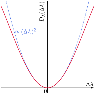
Figure 11: Schematic figure of the relative entropy $D_{\lambda}(\Delta\lambda)=D(\hat{\rho}(\lambda+\Delta\lambda)|\hat{\rho}(\lambda))$ for small $|\Delta\lambda|$ (red thick line), showing that $D_{\lambda}(0)=0$ and ${\rm d}D_{\lambda}(0)/{\rm d}\lambda=0$. Blue dashed line indicates a function proportional to $(\Delta\lambda)^{2}$, for comparison.

Appendix B Effective temperature in subsystem $B$

In Sec. III, we have found excellent agreement between statistical-mechanical quantities such as the thermodynamic entropy $S_{A}(\beta)$ and the internal energy $E_{A}(\beta)$ for an isolated subsystem $A$ and quantum-mechanical quantities such as the entanglement von Neumann entropy $\mathcal{S}_{A}(\lambda)$ and the energy $\mathcal{E}_{A}(\lambda)$ of a partitioned subsystem $A$ for a ground state of the whole system $A+B$, provided that the thermodynamic temperature $T=1/\beta$ in the former is set properly to the effective temperature $\mathcal{T}_{A}(\lambda)$ determined in the latter. A natural question is now how the effective temperature $\mathcal{T}_{B}(\lambda)$ of subsystem $B$ behaves. Here, $1/\mathcal{T}_{B}(\lambda)$ is defined as in Eq. (21) but with the energy $\mathcal{E}_{B}(\lambda)$ of subsystem $B$ instead of $\mathcal{E}_{A}(\lambda)$ of subsystem $A$ [note that $\mathcal{S}_{B}(\lambda)=\mathcal{S}_{A}(\lambda)$]. Because of the interaction term $\hat{V}_{AB}(\lambda)$, there exists quantum entanglement between subsystems $A$ and $B$. This is different from the case discussed in Sec. V.1.2, where no interactions are assumed between subsystems $X$ and $Y$, and hence $\mathcal{T}_{A}(\lambda)\not=\mathcal{T}_{B}(\lambda)$ is expected in general.

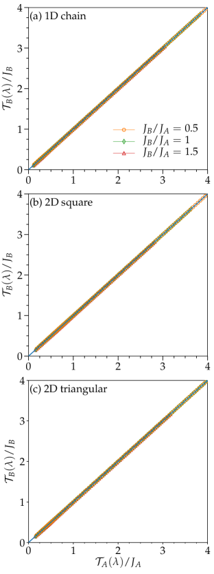
Figure 12: The effective temperature $\mathcal{T}_{B}(\lambda)/J_{B}$ of subsystem $B$ as a function of the effective temperature $\mathcal{T}_{A}(\lambda)/J_{A}$ of subsystem $A$ for the spin-1/2 antiferromagnetic Heisenberg model in (a) the two coupled 1D chains (i.e, two-leg ladder), (b) the two coupled 2D square lattice (i.e., bilayer square lattice), and (c) the two coupled 2D triangular lattice (i.e., bilayer triangular lattice) with $N_{A}=N_{B}=8$.

Figure 12 shows the effective temperature $\mathcal{T}_{B}(\lambda)/J_{B}$ of subsystem $B$ as a function of $\mathcal{T}_{A}(\lambda)/J_{A}$ for the three different lattices studied in Sec. III. We find that $\mathcal{T}_{A}(\lambda)/J_{A}\simeq\mathcal{T}_{B}(\lambda)/J_{B}$ even for $J_{B}/J_{A}\not=1$. Apparently, this relation is somewhat similar to the common temperature condition in thermodynamics, which is a consequence of the equilibrium between two subsystems. However, the important distinction is that here the microscopic energy scales $J_{A}$ and $J_{B}$ of subsystems $A$ and $B$, respectively, which are absent in thermodynamics, enter in the relation. Moreover, the relatively simple relation between $\mathcal{T}_{A}(\lambda)$ and $\mathcal{T}_{B}(\lambda)$ found here might be due to our setting of the Hamiltonian where $\hat{H}_{B}=(J_{B}/J_{A})\hat{H}_{A}$. Finally, we note that the same relation is exactly satisfied in the two analytical examples discussed in Sec. IV [see Eqs. (60) and (92)].

Appendix C Thermofield-double-like state

In terms of the Schmidt decomposition of the ground-state wavefunction $|\Psi_{0}(\lambda)\rangle$, the assumption in Eq. (109) along with Eq. (112) can be rephrased as

$$|\Psi_{0}(\lambda)\rangle\overset{!}{=}\sum_{n=1}^{D_{A}}\frac{{\rm e}^{-\mathcal{B}_{A}(\lambda)\epsilon^{A}_{n}/2}}{\sqrt{Z_{A}(\mathcal{B}_{A})}}|\psi^{A}_{n}\rangle_{A}|g_{n}\rangle_{B},$$ (119)

where $|\psi^{A}_{n}\rangle_{A}$ is the $n$th eigenstate of $\hat{H}_{A}$ with its eigenvalue $\epsilon_{n}^{A}$ and $\{|g_{n}\rangle_{B}\}$ is a orthonormal basis set of subsystem $B$. The purification of $\hat{\rho}_{A}^{\rm red}(\lambda)$ in Eq. (119) resembles to the thermofield double state [43]. Indeed, if the subsystem $B$ is selected to be identical to the subsystem $A$, the right hand side in Eq. (119) should reproduce the thermofield double state for the subsystem $A$ at temperature $1/\mathcal{B}_{A}(\lambda)$.

References

- von Neumann [2010] J. von Neumann, Proof of the ergodic theorem and the h-theorem in quantum mechanics, The European Physical Journal H 35, 201 (2010).
- Jensen and Shankar [1985] R. V. Jensen and R. Shankar, Statistical behavior in deterministic quantum systems with few degrees of freedom, Phys. Rev. Lett. 54, 1879 (1985).
- Tasaki [1998] H. Tasaki, From quantum dynamics to the canonical distribution: General picture and a rigorous example, Phys. Rev. Lett. 80, 1373 (1998).
- Kollar and Eckstein [2008] M. Kollar and M. Eckstein, Relaxation of a one-dimensional mott insulator after an interaction quench, Phys. Rev. A 78, 013626 (2008).
- Linden et al. [2009] N. Linden, S. Popescu, A. J. Short, and A. Winter, Quantum mechanical evolution towards thermal equilibrium, Phys. Rev. E 79, 061103 (2009).
- Short [2011] A. J. Short, Equilibration of quantum systems and subsystems, New Journal of Physics 13, 053009 (2011).
- Ikeda et al. [2015] T. N. Ikeda, N. Sakumichi, A. Polkovnikov, and M. Ueda, The second law of thermodynamics under unitary evolution and external operations, Annals of Physics 354, 338 (2015).
- Pappalardi et al. [2017] S. Pappalardi, A. Russomanno, A. Silva, and R. Fazio, Multipartite entanglement after a quantum quench, Journal of Statistical Mechanics: Theory and Experiment 2017, 053104 (2017).
- Deutsch [1991] J. M. Deutsch, Quantum statistical mechanics in a closed system, Phys. Rev. A 43, 2046 (1991).
- Srednicki [1994] M. Srednicki, Chaos and quantum thermalization, Phys. Rev. E 50, 888 (1994).
- Rigol et al. [2008] M. Rigol, V. Dunjko, and M. Olshanii, Thermalization and its mechanism for generic isolated quantum systems, Nature 452, 854 (2008).
- Nandkishore and Huse [2015] R. Nandkishore and D. A. Huse, Many-body localization and thermalization in quantum statistical mechanics, Annual Review of Condensed Matter Physics 6, 15 (2015).
- Iyoda et al. [2017] E. Iyoda, K. Kaneko, and T. Sagawa, Fluctuation theorem for many-body pure quantum states, Phys. Rev. Lett. 119, 100601 (2017).
- Deutsch [2018] J. M. Deutsch, Eigenstate thermalization hypothesis, Reports on Progress in Physics 81, 082001 (2018).
- Cassidy et al. [2011] A. C. Cassidy, C. W. Clark, and M. Rigol, Generalized thermalization in an integrable lattice system, Phys. Rev. Lett. 106, 140405 (2011).
- Shiraishi and Mori [2017] N. Shiraishi and T. Mori, Systematic construction of counterexamples to the eigenstate thermalization hypothesis, Phys. Rev. Lett. 119, 030601 (2017).
- Shibata et al. [2020] N. Shibata, N. Yoshioka, and H. Katsura, Onsager’s scars in disordered spin chains, Phys. Rev. Lett. 124, 180604 (2020).
- Popescu et al. [2006] S. Popescu, A. J. Short, and A. Winter, Entanglement and the foundations of statistical mechanics, Nature Physics 2, 754–758 (2006).
- Goldstein et al. [2006] S. Goldstein, J. L. Lebowitz, R. Tumulka, and N. Zanghì, Canonical typicality, Phys. Rev. Lett. 96, 050403 (2006).
- Sugita [2007] A. Sugita, On the basis of quantum statistical mechanics, Nonlinear Phenom. Complex Syst. 10, 192 (2007).
- Reimann [2007] P. Reimann, Typicality for generalized microcanonical ensembles, Phys. Rev. Lett. 99, 160404 (2007).
- Tasaki [2016] H. Tasaki, Typicality of thermal equilibrium and thermalization in isolated macroscopic quantum systems, Journal of Statistical Physics 163, 937–997 (2016).
- Sugiura and Shimizu [2012] S. Sugiura and A. Shimizu, Thermal pure quantum states at finite temperature, Phys. Rev. Lett. 108, 240401 (2012).
- Sugiura and Shimizu [2013] S. Sugiura and A. Shimizu, Canonical thermal pure quantum state, Phys. Rev. Lett. 111, 010401 (2013).
- Hyuga et al. [2014] M. Hyuga, S. Sugiura, K. Sakai, and A. Shimizu, Thermal pure quantum states of many-particle systems, Phys. Rev. B 90, 121110 (2014).
- Ryu and Hatsugai [2006] S. Ryu and Y. Hatsugai, Entanglement entropy and the berry phase in the solid state, Phys. Rev. B 73, 245115 (2006).
- Li and Haldane [2008] H. Li and F. D. M. Haldane, Entanglement spectrum as a generalization of entanglement entropy: Identification of topological order in non-abelian fractional quantum hall effect states, Phys. Rev. Lett. 101, 010504 (2008).
- Qi et al. [2012] X.-L. Qi, H. Katsura, and A. W. W. Ludwig, General relationship between the entanglement spectrum and the edge state spectrum of topological quantum states, Phys. Rev. Lett. 108, 196402 (2012).
- Furukawa and Kim [2011] S. Furukawa and Y. B. Kim, Entanglement entropy between two coupled tomonaga-luttinger liquids, Phys. Rev. B 83, 085112 (2011).
- Lundgren et al. [2013] R. Lundgren, Y. Fuji, S. Furukawa, and M. Oshikawa, Entanglement spectra between coupled tomonaga-luttinger liquids: Applications to ladder systems and topological phases, Phys. Rev. B 88, 245137 (2013).
- Poilblanc [2010] D. Poilblanc, Entanglement spectra of quantum heisenberg ladders, Phys. Rev. Lett. 105, 077202 (2010).
- Läuchli and Schliemann [2012] A. M. Läuchli and J. Schliemann, Entanglement spectra of coupled spin chains in a ladder geometry, Phys. Rev. B 85, 054403 (2012).
- Parisen Toldin and Assaad [2018] F. Parisen Toldin and F. F. Assaad, Entanglement hamiltonian of interacting fermionic models, Phys. Rev. Lett. 121, 200602 (2018).
- Bayat et al. [2014] A. Bayat, H. Johannesson, S. Bose, and P. Sodano, An order parameter for impurity systems at quantum criticality, Nature Communications 5, 3784 (2014).
- Shirakawa and Yunoki [2016] T. Shirakawa and S. Yunoki, Density matrix renormalization group study in energy space for a single-impurity anderson model and an impurity quantum phase transition, Phys. Rev. B 93, 205124 (2016).
- Lou et al. [2011] J. Lou, S. Tanaka, H. Katsura, and N. Kawashima, Entanglement spectra of the two-dimensional affleck-kennedy-lieb-tasaki model: Correspondence between the valence-bond-solid state and conformal field theory, Phys. Rev. B 84, 245128 (2011).
- Chang et al. [2019] P.-Y. Chang, X. Chen, S. Gopalakrishnan, and J. H. Pixley, Evolution of entanglement spectra under generic quantum dynamics, Phys. Rev. Lett. 123, 190602 (2019).
- Peschel and Chung [2011] I. Peschel and M.-C. Chung, On the relation between entanglement and subsystem hamiltonians, EPL (Europhysics Letters) 96, 50006 (2011).
- Dalmonte et al. [2018] M. Dalmonte, B. Vermersch, and P. Zoller, Quantum simulation and spectroscopy of entanglement hamiltonians, Nature Physics 14, 827 (2018).
- Giudici et al. [2018] G. Giudici, T. Mendes-Santos, P. Calabrese, and M. Dalmonte, Entanglement hamiltonians of lattice models via the bisognano-wichmann theorem, Phys. Rev. B 98, 134403 (2018).
- Mendes-Santos et al. [2020] T. Mendes-Santos, G. Giudici, R. Fazio, and M. Dalmonte, Measuring von neumann entanglement entropies without wave functions, New Journal of Physics 22, 013044 (2020).
- Kaufman et al. [2016] A. M. Kaufman, M. E. Tai, A. Lukin, M. Rispoli, R. Schittko, P. M. Preiss, and M. Greiner, Quantum thermalization through entanglement in an isolated many-body system, Science 353, 794–800 (2016).
- Fano [1957] U. Fano, Description of states in quantum mechanics by density matrix and operator techniques, Rev. Mod. Phys. 29, 74 (1957).
- White [2009] S. R. White, Minimally entangled typical quantum states at finite temperature, Phys. Rev. Lett. 102, 190601 (2009).
- Lieb and Yngvason [1999] E. H. Lieb and J. Yngvason, The physics and mathematics of the second law of thermodynamics, Physics Reports 310, 1–96 (1999).
- Gilchrist et al. [2005] A. Gilchrist, N. K. Langford, and M. A. Nielsen, Distance measures to compare real and ideal quantum processes, Phys. Rev. A 71, 062310 (2005).
- Zhang et al. [2020] J. Zhang, P. Calabrese, M. Dalmonte, and M. A. Rajabpour, Lattice Bisognano-Wichmann modular Hamiltonian in critical quantum spin chains, SciPost Phys. Core 2, 7 (2020).
- Unruh [1976] W. G. Unruh, Notes on black-hole evaporation, Phys. Rev. D 14, 870 (1976).
- Crispino et al. [2008] L. C. B. Crispino, A. Higuchi, and G. E. A. Matsas, The unruh effect and its applications, Rev. Mod. Phys. 80, 787 (2008).
- Lee [1990] C. T. Lee, Two-mode squeezed states with thermal noise, Phys. Rev. A 42, 4193 (1990).
- Bardeen et al. [1957] J. Bardeen, L. N. Cooper, and J. R. Schrieffer, Theory of superconductivity, Phys. Rev. 108, 1175 (1957).
- Wehrl [1978] A. Wehrl, General properties of entropy, Rev. Mod. Phys. 50, 221 (1978).
- Blanco et al. [2013] D. D. Blanco, H. Casini, L.-Y. Hung, and R. C. Myers, Relative entropy and holography, Journal of High Energy Physics 2013, 10.1007/jhep08(2013)060 (2013).
- Sugiura and Shimizu [2014] S. Sugiura and A. Shimizu, New formulation of statistical mechanics using thermal pure quantum states, in Physics, Mathematics, and All that Quantum Jazz, Kinki University Series on Quantum Computing, Vol. 9, edited by S. Tanaka, M. Bando, and U. Güngördü (World Scientific, 2014) pp. 245–257.
- Shimizu and Miyadera [2001] A. Shimizu and T. Miyadera, Energies and collapse times of symmetric and symmetry-breaking states of finite systems with a u(1) symmetry, Phys. Rev. E 64, 056121 (2001).
- Shimizu and Miyadera [2002] A. Shimizu and T. Miyadera, Stability of quantum states of finite macroscopic systems against classical noises, perturbations from environments, and local measurements, Phys. Rev. Lett. 89, 270403 (2002).
- Suzuki [1985] M. Suzuki, Thermo field dynamics in equilibrium and non-equilibrium interacting quantum systems, Journal of the Physical Society of Japan 54, 4483 (1985).
- Verstraete et al. [2004] F. Verstraete, J. J. García-Ripoll, and J. I. Cirac, Matrix product density operators: Simulation of finite-temperature and dissipative systems, Phys. Rev. Lett. 93, 207204 (2004).
- Zwolak and Vidal [2004] M. Zwolak and G. Vidal, Mixed-state dynamics in one-dimensional quantum lattice systems: A time-dependent superoperator renormalization algorithm, Phys. Rev. Lett. 93, 207205 (2004).
- Feiguin and White [2005] A. E. Feiguin and S. R. White, Finite-temperature density matrix renormalization using an enlarged hilbert space, Phys. Rev. B 72, 220401 (2005).
- Wu and Hsieh [2019] J. Wu and T. H. Hsieh, Variational thermal quantum simulation via thermofield double states, Phys. Rev. Lett. 123, 220502 (2019).
- Long et al. [2003] M. W. Long, P. Prelovšek, S. El Shawish, J. Karadamoglou, and X. Zotos, Finite-temperature dynamical correlations using the microcanonical ensemble and the lanczos algorithm, Phys. Rev. B 68, 235106 (2003).
- Okamoto et al. [2018] S. Okamoto, G. Alvarez, E. Dagotto, and T. Tohyama, Accuracy of the microcanonical lanczos method to compute real-frequency dynamical spectral functions of quantum models at finite temperatures, Phys. Rev. E 97, 043308 (2018).
- White [1992] S. R. White, Density matrix formulation for quantum renormalization groups, Phys. Rev. Lett. 69, 2863 (1992).
- Johri et al. [2017] S. Johri, D. S. Steiger, and M. Troyer, Entanglement spectroscopy on a quantum computer, Phys. Rev. B 96, 195136 (2017).
- Islam et al. [2015] R. Islam, R. Ma, P. M. Preiss, M. Eric Tai, A. Lukin, M. Rispoli, and M. Greiner, Measuring entanglement entropy in a quantum many-body system, Nature 528, 77 (2015).
- Umegaki [1962] H. Umegaki, Conditional expectation in an operator algebra. iv. entropy and information, Kodai Math. Sem. Rep. 14, 59 (1962).
- Lindblad [1973] G. Lindblad, Entropy, information and quantum measurements, Communications in Mathematical Physics 33, 305 (1973).
- Sagawa [2012] T. Sagawa, Second law-like inequalities with quantum relative entropy: An introduction, in Lectures on Quantum Computing, Thermodynamics and Statistical Physics, Kinki University Series on Quantum Computing, Vol. 8, edited by M. Nakahara and S. Tanaka (World Scientific, 2012) pp. 125–190.