Unified Framework for the Adaptive
Operator Selection of Discrete Parameters

Abstract

We conduct an exhaustive survey of adaptive selection of operators (AOS) in Evolutionary Algorithms (EAs). We simplified the AOS structure by adding more components to the framework to built upon the existing categorisation of AOS methods. In addition to simplifying, we looked at the commonality among AOS methods from literature to generalise them. Each component is presented with a number of alternative choices, each represented with a formula. We make three sets of comparisons. First, the methods from literature are tested on the bbob test bed with their default hyper parameters. Second, the hyper parameters of these methods are tuned using an offline configurator known as irace. Third, for a given set of problems, we use irace to select the best combination of components and tune their hyper parameters.

I Introduction

Evolutionary algorithms (EAs) are derivative free algorithms that have proven to be useful as optimisation techniques [1] for a wide range of problems in different application areas [2, 3, 4, 5, 6, 7]. They are known to guarantee near optimum solution for a given problem. The nature of the optimisation problem considered is usually black-box where the algorithm is unaware of the properties of the problem such as continuous, convex, unimodal, multimodal, separable, quadratic, high dimensional, gaussian noise, and so on.

Their performance highly depend on the choice of parameter values. Thus, it is important to employ a parameter selection method that selects the near-optimal parameter values of the algorithm. The parameters with finite or infinite number of choices are known as discrete or continuous parameters respectively. The type of crossover operator such as one-point and multi-point in Genetic Algorithm is a discrete parameter whereas crossover rate in the range $[0.0,1.0]$ is a continuous parameter. We do not know in advance the best setting of the EA given the problem and have limited knowledge about effect of parameters on EA performance. Thus, to decide the values of parameters either tuning or controlling can be used. Tuning uses offline configurators that refines the optimal configurations after a few runs (Sequential Parameter Optimisation [8]) or discards the configurations if they are worse than others based on the statistical evidence (irace [9]). The controlling methods use deterministic, self-adaptation or adaptation methods. In case of parameter tuning (offline method), the parameters are tuned and trained on a parameter set. Once the parameters are tuned the values do not change during the run of the algorithm. On the contrary, parameter control (online method) has no training phase and parameter values are adapted and learned during the run of the algorithm. Both these methods have limitations. On the one hand, offline configurators need extra budget in terms of the function evaluations and do not generalise well on variety of problems, online tuning on the other hand slows down the learning process due to slow exploration of the parameter search space. A survey on parameter tuning and control can be found in [10, 11]. In this paper we have used the properties of both offline tuning and online control to learn the optimal parameter values during the run of an algorithm.

We focus on the adaptive selection of discrete parameters (or operators) during the run, known as Adaptive Operator Selection (AOS). The concept of AOS was introduced around 1990s [12]. Since then, there have been various AOS methods proposed in literature that vary broadly in various aspects such as amount of information to use from the past performance of the algorithm and whether including previous quality in the learning process is an effective approach. It has been classified into two components, Credit Assignment (CA) and Operator Selection (OS) [13]. CA involves a definition based on the fitness achievement over a solution. The most commonly used CA technique is fitness improvement from parent to offspring. OS takes the information captured by CA and estimates the quality of each operator followed by calculating its probability. In the end, a selection technique is employed to select an operator for evolving a parent based on probability assigned to each operator. The same selection technique is used to evolve all parents in a generation. As this process progresses, algorithm learns more and more about the landscape and after a number of generations, this process moves the solutions in a particular search direction. [14] presents AOS component coupled with Adaptive Operator Management (AOM). Authors explored the hyper-parameter choices for two well-known AOS method: Compass [15] and Ex-DMAB [16]. The exploration of choices is limited to type of window and hyper-parameters of these two AOS methods. They introduced the concept of AOM where operators are unborn, alive or dead based on their performance criteria. It decided whether an operator is important for current stage or not. [17] makes choices for an AOS method [15] in order to balance exploration and exploitation concluding that adaptive methods are better than static methods. A survey on adaptive methods can be found in [18].

Many novel AOS methods can be designed by combining different components of existing AOS methods. There can be many combinations possible from the existing methods that are not tested as an AOS method. To test the efficiency of these methods as an AOS method, this paper presents a unified AOS framework that builds upon the existing classification of an AOS method [19]. This is done by analysing multiple AOS methods from the literature to design a simplified framework. The AOS methods used to build the framework are originally proposed in the literature to tune the parameters of various EAs such as genetic algorithms and differential evolution. The framework consist of multiple choices for each AOS component. Some of the choices are inspired from Reinforcement Learning utilised to adapt parameters of different EAs. The framework can be utilised to explore different combinations of the AOS components’ choices. As an estimate, we can generate more than $5000$ novel AOS methods from the framework. It can also be used to replicate various known AOS methods from the literature. An AOS method is build from the framework by setting the component choices and fixing the values of their parameters. In order to make the framework widely applicable, choices with diverse properties are included such as immediate progress to far-sighted progress, focusing on the clustered achievement to the outliers, etc. In addition to this, some novel choices are added to the components and each choice is generalised. In the process of generalisation, a number of hyper-parameters are introduced within the choices. The resultant framework is applicable for the online adaptation of discrete parameters of an evolutionary algorithm.

As the framework consists of various AOS methods with their hyper-parameters, an offline configurator is employed to select an optimal AOS method and tune its hyper-parameters. Thus, we present a combination of the online adaptive methods with an offline configurator to improve the search performance of differential evolution (DE). Along with selecting an AOS method with its parameters, the tuner also decides the parameters of the DE algorithm. We have utilised the framework to find a suitable tuned AOS method to adapt nine commonly used mutation strategies in DE on the bbob benchmark set. The resultant framework is flexible enough to replace DE with any EA to tune its discrete set of parameters. It is build upon the existing classification of AOS method [19]. The following three tasks are performed to achieve a unified framework of AOS methods combined with an offline configurator:

• We build upon the existing classification [17] by identifying the new components to simplify the structure of AOS. AOS methods are known to have two major components, credit assignment (assigning reward to an operator) and operator selection (assigning probability to each operator based on quality). We have used this existing classification and further classified these components. The classification is shown in figure 1

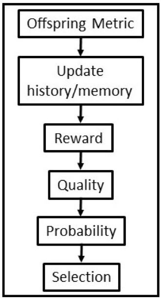
  Figure 1: Adaptive Operator Selection classification

  

• A simplified taxonomy is presented that consists of five components with different heuristics as their choices. Thus, the framework consists of an in-depth formulation of AOS components with a generalised structure. In order to make the framework widely applicable we include the choices with diverse properties in each component. Most of the choices are inspired from Evolutionary domain which consists of Reinforcement earning inspired algorithms and thus the architecture can be used in Machine Learning domain as well. We consider immediate progress to far-sighted progress; focusing on the clustered achievement to the outliers. These papers have not explored the possible combinations and their possibility to explore the search space better. There can be many more combinations possible from literature which are never explored and might results in a novel combination that results in much better results. Each AOS component with its choices is shown in figure 2

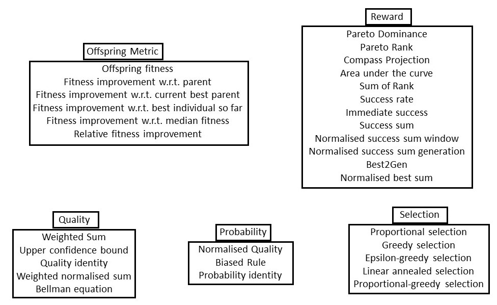
  Figure 2: Adaptive Operator Selection component choices

  

• The resultant framework consists of various AOS designs, out of which one needs to be selected to perform online tuning of parameters in an EA. Thus, a tuner (a meta-leaner) is employed to find a near optimal configuration setting or combination of choices for a given set of problems. A well-known offline configurator known as irace is used for this purpose. An AOS method has its own parameters to be tuned which do not directly impact the problem solution space. Thus, an offline configurator can be utilised efficiently to give a static value for these hyper-parameters. To tune these hyper-parameters we employ the same tuner in combination with the framework. The role of irace is to offline select a combination of component choices given a set of problems and tune the hyper-parameters of the selected AOS method along with the parameters of DE.

Figure 3 shows the simplified training procedure of the framework using an offline tuner irace. irace samples a configuration from the component space and its hyper-parameter space related to the selected choices. It also samples a configuration from the DE parameter space. These choices remain static while the algorithm runs on a selected problem instance selected from a training set. During this run, the AOS method formed by component choices selected by irace online tunes the mutation strategy of DE. At the end of an EA run, the best seen fitness value is sent to the irace in the form of cost to make an informed decision on the optimal choices. This describes a single step of irace. This process is followed repeatedly until a budget given to irace is exhausted and the configuration that performed best is returned. This configuration consists of a choice from each AOS component, its tuned hyper-parameters and parameter values of DE.

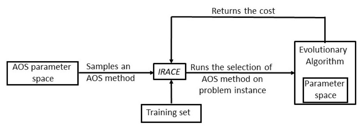
Figure 3: Unified Adaptive Operator Selection architecture

II Preliminaries

II-A Problem definition

We assume a single-objective problem, where the cost of a solution $x\in X$ is given by $f\colon X\to\mathbb{R}$, which w.l.o.g, must be minimized.

We assume an algorithm with a set of alternative operators $\textit{op}\in\textit{Op}$. An operator is a function $\textit{op}\colon X\to X$ that takes a number of solutions (parents) and returns one or more solutions (offsprings). For instance, crossover operator in Genetic Algorithms is an operator that takes two or more solutions from the parent population to generate offsprings.

The proposed framework can select different crossover operator as well tune crossover rate. Also, it is independent on the number of solutions the operator deals with. That is, it imposes no restriction on number of solutions used by an operator to generate a certain number of solutions. Thus, this architecture is applicable for any kind of operator which has discrete number of choices, as long as one parent is replaced by one offspring.

II-B Differential Evolution

To test our architecture we adapt the operators of DE [20]. It is a population-based algorithm that uses a mutation strategy to create an offspring solution $\vec{u}_{i}$. A mutation strategy is a linear combination of three or more parent solutions $\vec{x}_{i}$, where $i$ is the index of a solution in the current population. Some mutation strategies are good at exploration and others at exploitation, and it is well-known that no single strategy performs best for all problems and for all stages of a single run. A survey of development in DE can be found in [21]. In this paper, we consider following frequently used mutation strategies:

“rand/1”:	$\vec{u}_{i}=\vec{x}_{r_{1}}+F\cdot(\vec{x}_{r_{2}}-\vec{x}_{r_{3}})$
“rand/2”:	$\vec{u}_{i}=\vec{x}_{r_{1}}+F\cdot(\vec{x}_{r_{2}}-\vec{x}_{r_{3}}+\vec{x}_{r_{4}}-\vec{x}_{r_{5}})$
“rand-to-best/2”:	$\vec{u}_{i}=\vec{x}_{r_{1}}+F\cdot(\vec{x}_{\text{best}}-\vec{x}_{r_{1}}+\vec{x}_{r_{2}}-\vec{x}_{r_{3}}+\vec{x}_{r_{4}}-\vec{x}_{r_{5}})$
“curr-to-rand/1”:	$\vec{u}_{i}=\vec{x}_{i}+F\cdot(\vec{x}_{r_{1}}-\vec{x}_{i}+\vec{x}_{r_{2}}-\vec{x}_{r_{3}})$
“curr-to-pbest/1”:	$\vec{u}_{i}=\vec{x}_{i}+F\cdot(\vec{x}_{pbest}-\vec{x}_{i}+\vec{x}_{r_{1}}-\vec{x}_{r_{2}})$
“curr-to-pbest/1 (archived)”:	$\vec{u}_{i}=\vec{x}_{i}+F\cdot(\vec{x}_{pbest}-\vec{x}_{i}+\vec{x}_{r_{1}}-\vec{x}_{archive})$
“best/1”:	$\vec{u}_{i}=\vec{x}_{best}+F\cdot(\vec{x}_{r_{1}}-\vec{x}_{r_{2}})$
“best/2”:	$\vec{u}_{i}=\vec{x}_{best}+F\cdot(\vec{x}_{r_{1}}-\vec{x}_{r_{2}}+\vec{x}_{r_{3}}-\vec{x}_{r_{4}})$
“curr-to-best/1”:	$\vec{u}_{i}=\vec{x}_{i}+F\cdot(\vec{x}_{best}-\vec{x}_{i}+\vec{x}_{r_{1}}-\vec{x}_{r_{2}})$

$F$ is a scaling factor, $\vec{u}_{i}$ and $\vec{x}_{i}$ are the $i$-th offspring and parent solutions in the population, respectively, $\vec{x}_{\text{best}}$ is the best parent in the population, and $r_{1}$, $r_{2}$, $r_{3}$, $r_{4}$, and $r_{5}$ are randomly generated mutually exclusive indexes within $[1,NP]$, where $NP$ is the population size. An additional numerical parameter, the crossover rate ($CR\in[0,1]$), determines whether the mutation strategy is applied to each dimension of $\vec{x}_{i}$ to generate $\vec{u}_{i}$. At least one dimension of each $\vec{x}_{i}$ vector is mutated.

rand/1 and rand/2 are known to explore the search space whereas best/1 and best/2 exploit the neighborhood of the best candidate in the population. curr-to-pbest/1 and curr-to-pbest/1(archived), modifications of curr-to-best/1, are proposed as a novel operator in JaDE algorithm. We decided to include these mutation strategies involved in JaDE as they balance the exploration and exploitation of the solution space resulting in competitive performance compared to the other DE variants . We also include two other popular mutation strategies to increase the robustness of the framework. These are curr-to-rand/1 and rand-to-best/2, known to explore the neighborhood of current parent and best parent in the current population respectively.

III Components of the proposed framework for AOS

In this section the components of the proposed framework are discussed in detail. It consists of five components each with a number of generalised choices. The five components are offspring metric (OM), reward ($r_{g+1,op}$), quality ($q_{g+1,op}$), probability ($p_{g+1,op}$) assignment and selection mechanism ($op_{g+1}$). We consider individual level control that is in a generation an operator is selected for each parent. At the end of the generation, OM assigns a value to each offspring according to the improvement gained with the operator application. To prepare the selection of operators for the population in the next generation, reward, quality and probability of each operator are updated, according to the OM values. In the end, based on the probability values of each operator, the selection method is invoked to select the operator for each parent to produce offspring. Further, we discuss each of the component choices one by one in detail.

III-A Offspring Metric

We define an OM as a function of some statistics on population fitness. The metric, mathematically represented as ($\textit{OM}(g,k,op)$), assigns a $k$-th improved value to the $i$-th improved solution (offspring) $x_{i,op}$ generated after using operator op. If there is no improvement, $0.0$ metric value is assigned to the offspring. That implies that the offspring ($\textit{OM}(g,k,op)$) is as good as its parent. OM value depends on the parent fitness, the offspring fitness and other significant references shown in table I. The table shows seven offspring metrics all of which are designed to be maximised when the objective function is a minimisation problem. That is, for an $\textit{OM}(g,k,op)$, the higher the value of $i$-th offspring, the better the offspring is.

We store all OM in memory that can be of two types, generation memory and window memory. The generation memory stores six OM values for each offspring in each generation. These values are shown in fig. I. As the algorithm progresses, the size of generation memory grows. A window memory of size $\mathcal{W}$ is formed using the generation memory. Each entry in the window consists of six values resulting from OM. The window memory stores these six metric values of an offspring only if it improves over its parent. In other words, it stores a finite set of OM generated by any operator. Initially, the window is filled as the offsprings are generated. Once the window is filled, the new improved offspring generated by an operator is inserted in First In First Out (FIFO) manner such that the offspring from the window generated by the same operator to enter first is removed and new offspring metric data is put at top of the window. If there is no application of that operator present in the window, the worst offspring data is removed. The generation memory and window memory are updated at the end of each generation. The data from generation memory can be utilised either for fix number of generations or for fix number of operator applications described below:

• Dynamic number of operator applications ($\max_{\text{gen}}$ as a parameter): The OM values produced by an operator in the last fix number of $\max_{\text{gen}}$ generation(s) are taken into account. It is important to note that the number of applications of each operator can vary in each generation. Thus, in $\max_{\text{gen}}$ number of generations the number of total applications of an operator can be different from others.

• Fix number of operator applications ($fix_{\text{appl}}$ as parameter): In this case the last fixed number of operator applications are considered. The generation span depends on the improved offsprings in each generation and is not known in advance.

Table I: Offspring Metrics ($\textit{OM}(g,k,op)$)

Name	Definition
Offspring fitness	$$-f(u_{i,op})$$ (1)
Fitness improvement w.r.t. parent	$$\max\{0,f(x_{i})-f(u_{i,op})\}$$ (2)
Fitness improvement w.r.t. current best parent	$$\max\{0,f_{best}-f(u_{i,op})\}$$ (3)
Fitness improvement w.r.t. best individual so far	$$\max\{0,f_{bsf}-f(u_{i,op})\}$$ (4)
Fitness improvement w.r.t. median fitness	$$\max\{0,f_{median}-f(u_{i,op})\}$$ (5)
Relative fitness improvement	$$\left(\frac{f_{bsf}}{f(u_{i,op})}\right)\cdot\max\{0,(f(x_{i})-f(u_{i,op}))\}$$ (6)

Equation 1 [22, 23, 24, 25, 26, 27, 28] defines the offspring fitness. For the minimisation problem, this metric assigns the offspring an OM as the negative of the raw fitness. In case of the maximisation problem, the raw fitness value should be considered.

The next four equations 2 – 5 define the OM as the difference between the fitness of an offspring generated by the application of operator $op$ and a reference point. The reference points considered in this study are parent fitness ($f(x_{i})$) [23, 29, 30, 16, 19, 31, 32, 22, 33, 34, 35, 36, 37, 15, 38], best parent fitness ($f_{best}$) [23, 30, 12], best individual fitness so far ($f_{bsf}$) and median population fitness ($f_{median}$) [39, 40, 41]. Getting a value $0$ shows that there is no significant improvement in the offspring from a reference point. These four metrics follow the following rule: the farther the offspring from the reference point, the higher the OM will be.

The offspring fitness improvement shown in equation 2 has been most widely used in the literature showing its significance in giving useful information of an operator. Among these four metrics, we propose to include the best seen candidate as a reference point shown in equation 4. It is an important reference as it gives a search direction for the exploitation in the neighborhood of the best so far candidate. In this case, an operator that produce an offspring with higher fitness in reference to the best so far candidate gets higher reward value compared to the operator producing offspring with relatively lower improvement.

Relative fitness improvement defined in equation 6 was originally proposed in [42] and later used in [43] as part of an AOS method. It takes into account the fitness improvement from parent to offspring along with the best so far candidate fitness.

III-B Reward

The reward given to an operator op at generation $g+1$, represented as $r_{g+1,op}$, gives a measure of achievement of an operator. It goes beyond the current performance of an operator using either generation or memory window. In a run of EA, it is a function of one of the selected OM. The reward assigned to an operator is maximised as the OM is designed to be maximised. That means if an operator has performed better than another operator, then former should get higher reward compared to the latter for any selected OM.

We present a generalised classification of the reward definitions from the literature shown in table LABEL:tab:Reward. They utilise an OM definition for an operator in a specifically defined manner. Some make the use of direct fitness values such as diversity and quality, weighted fitness average and best OM; others using fitness based score such as ranking and count of improved OM. Reward combines one or two of these statistics, thus learning from limited amount of information available from the fitness landscape.

Some authors consider rewarding ancestors of a well-performing operator [44, 33] in addition to rewarding the current operator itself; others do not consider such a case [22]. By ancestor we mean the operators that lead to the good performance of current operator. We decided not to include that option in the classification as [33] suggests that it sometimes degrades the results. In the framework, any method that involves clock time [24] is replaced by function evaluations in some cases. The framework updates reward at the end of each generation that is contrary to the methods that chose to update reward after a certain number of generations [45]. This implies that there is no update on AOS components for few generations because this can lead to loss of information. [35] introduces the idea of removing and adding operators from a storage called credit registry in an AOS. We do not maintain such a registry in the framework with the intuition that eventually an AOS can learn to select the optimal operator from a list of operators depending on the current stage of an EA.

The reward choices are divided into the following five categories: fitness diversity and quality, comparison based, successful operator applications, fitness sum and best offspring. The choices under these categories share similar properties. Fitness diversity and quality reward choices are made with the selected OM diversity and quality for a fix number of applications, choices under comparison based category involve ranking the OM from the window memory, successful operator applications comprise of the number of OM resulting from successful operator application, choices in fitness sum simply add the raw OM values and lastly best offspring category consists of choices formed with the best solution fitness in a generation combined from a certain number of generations.

Table II: Reward ($r_{g+1,op}$)

Definition	Parameters
Fitness Diversity and Quality
Pareto Dominance $$\frac{\mbox{PD }(o_{op}^{fix_{\text{appl}}})}{\sum_{j=1}^{K}\mbox{PD }(o_{j}^{fix_{\text{appl}}})}$$ (7)	$fix_{\text{appl}}$
Pareto Rank $$\frac{\mbox{PR }(o_{op}^{fix_{\text{appl}}})}{\sum_{j=1}^{K}\mbox{PR }(o_{j}^{fix_{\text{appl}}})}$$ (8)	$fix_{\text{appl}}$
Compass Projection $$|o_{op}^{fix_{\text{appl}}}|\cdot\cos(\alpha_{op})-\min_{j=1}^{K}|o_{op}^{fix_{\text{appl}}}|\cdot\cos(\alpha_{j})$$ (9)	$\theta$, $fix_{\text{appl}}$
Comparison (Rank)
Area Under the Curve $$\mbox{Area under the curve based on the rank of }\textit{OM}(g,k,op)$$ (10)	$D$,$\mathcal{W}$
Sum of Rank $$\frac{\sum_{r(\textit{OM}(g,k,op))}D^{r(\textit{OM}(g,k,op))}(\mathcal{W}-r(\textit{OM}(g,k,op)))}{\sum_{r=1}^{\mathcal{W}}D^{r(\textit{OM}(g,k,op))}(\mathcal{W}-r(\textit{OM}(g,k,op)))}$$ (11)	$D$,$\mathcal{W}$
Successful operator applications
Success Rate $$\sum_{t=g}^{g-(\max_{\text{gen}}-1)}\left(\frac{{(n_{succ,op}^{t})}^{\gamma}+Frac*\sum_{j=1}^{K}n_{succ,j}^{t}}{n_{succ,op}^{t}+n_{fail,op}^{t}}\right)+\epsilon$$ (12)	$\max_{\text{gen}},\epsilon$ $\gamma$,$Frac$
Immediate Success $$\frac{n_{succ,op}^{g}}{NP}$$ (13)	-
Fitness Sum
Success Sum $$\frac{\sum_{t=g}^{g-(\max_{\text{gen}}-1)}\sum_{i=1}^{n_{succ,op}^{t}}\textit{OM}(t,i,op)}{\sum_{t=g}^{g-(\max_{\text{gen}}-1)}n_{succ,op}^{t}+n_{fail,op}^{t}}$$ (14)	$\max_{\text{gen}}$
Normalised Success Sum Window $$\frac{\frac{\sum_{k=1}^{n_{\textit{op}}}\textit{OM}(t,k,op)}{n_{\textit{op}}}}{\left(Best_{j=1}^{K}\frac{\sum_{k=1}^{n_{j}}\textit{OM}(t,k,j)}{n_{j}}\right)^{\omega}}$$ (15)	$\omega$,$\mathcal{W}$
Normalised Success Sum Generation $$\sum_{t=g}^{g-(\max_{\text{gen}}-1)}{\frac{\sum_{i=1}^{n_{succ,op}^{t}}\textit{OM}(t,i,op)}{n_{succ,op}^{t}+n_{fail,op}^{t}}}$$ (16)	$\max_{\text{gen}}$
Best offspring
Best2Gen $$C*\frac{Best_{i=1}^{n_{succ,op}^{g}}\textit{OM}(g,i,op)-Best_{i=1}^{n_{succ,op}^{g-1}}\textit{OM}(g-1,i,op)}{(Best_{i=1}^{n_{succ,op}^{g-1}}\textit{OM}(g-1,i,op))^{\alpha}*|(n_{succ,op}^{g}+n_{fail,op}^{g})-(n_{succ,op}^{g-1}+n_{fail,op}^{g-1})|^{\beta}}$$ (17)	$C$ $\beta,\alpha$
Normalised Best Sum $$\frac{\frac{1}{\max_{\text{gen}}}\sum_{t=g}^{g-(\max_{\text{gen}}-1)}{Best_{i=1}^{n_{succ,op}^{t}}\textit{OM}(t,i,op)}^{\rho}}{(Best_{j=1}^{K}\{\sum_{t=g}^{g-(\max_{\text{gen}}-1)}Best_{i=1}^{n_{succ,k}^{t}}\textit{OM}(t,i,j)\})^{\alpha}}$$ (18)	$\alpha,\rho$ $\max_{\text{gen}}$

Fitness Diversity and Quality This category includes the diversity (standard deviation) and quality (average) over an OM, combined in different manner. The three definitions consider fix number of operator applications, $fix_{\text{appl}}$, extracted from generation memory. These two statistics are represented as a coordinate ($o_{op}^{fix_{\text{appl}}}$) in two dimensional space for each operator op shown in the equation below:

$$\begin{split}o_{op}^{fix_{\text{appl}}}&=(div_{i=k}^{k-({fix_{\text{appl}}}-1)}\textit{OM}(g,i,op),\\ &\qquad qual_{i=k}^{k-(fix_{\text{appl}}-1)}\textit{OM}(g,i,op))\end{split}$$ (19)

The diversity $div$ and quality $qual$ of OM for an operator op are calculated for last $fix_{\text{appl}}$ number of applications.

Pareto Dominance (PD) on ($o_{op}^{fix_{\text{appl}}}$) shown in equation LABEL:DQ1 [35] counts the number of operators that are dominated by op. It is normalised by the sum of $k$ operators’ reward values. The best operator corresponds to the highest value of PD indicating that it generated maximum number of offspring in last certain number of generations compared to other operators.

Pareto Rank (PR) on ($o_{op}^{fix_{\text{appl}}}$) shown in equation LABEL:DQ2 [35] method counts the number of operators that dominate op. The operator with the least PR value is the best of all operators. Operators with a PR value of $0$ belong to the Pareto frontier. Both PD and PR encourage non-dominated operators.

In equation LABEL:DQ3, proposed in [15], the projection of a coordinate $o_{op}^{fix_{\text{appl}}}$is taken on a plane represented by an angle $\theta$ (a hyper-parameter). This angle defines the trade-off between exploration and exploitation. Thus, the mathematical formulation of projection is given by $|o_{op}^{fix_{\text{appl}}}|\cdot\cos(\alpha_{\textit{op}})$ where,

$$\begin{split}|o_{op}^{fix_{\text{appl}}}|&=\biggl{\{}({div_{i=k}^{k-(fix_{\text{appl}}-1)}\textit{OM}(g,i,op)})^{2}\\ &\qquad+({qual_{i=k}^{k-(fix_{\text{appl}}-1)}\textit{OM}(g,i,op)})^{2}\biggl{\}}^{1/2}\end{split}$$ (20)

$$\alpha_{\textit{op}}=atan\left(\frac{qual_{i=k}^{k-(fix_{\text{appl}}-1)}\textit{OM}(g,i,\textit{op})}{div_{i=k}^{k-(fix_{\text{appl}}-1)}\textit{OM}(g,i,\textit{op})}\right)-\theta\mbox{ and }$$ (21)

$\alpha_{\textit{op}}$ is the angle between the plane and the coordinate. Compass evaluates the performance of operators by considering not only the fitness improvements from parent to offspring, but also the way they modify the diversity of the population. This was later combined with dynamic multi-armed bandit [34, 35] for adaptive selection of the operators in differential evolution.

Comparison (Rank) The two definitions in this category assign a rank to each operator in the window of size $\mathcal{W}$according to OM values. These ranks are then decayed using hyper-parameter $D$ to prioritise the operators according to their ranks. As ranking of OM is involved and not the direct OM values, both methods under this category are invariant with respect to the linear scaling of the fitness function. That is, their behavior, when applied on a given fitness function $f$, is exactly the same when applied to a fitness function defined by $(a\cdot f)$, for any $a>0$.

Area Under the Curve (AUC) LABEL:R1 [37] plots a Receiver Operator Characteristic (ROC) curve for each operator by scanning the decayed ranking of OM from a window memory. The area is taken as a reward of each operator.

Sum of rank (SR) LABEL:R2 [37] assigns the operators with the sum of the decayed ranks of the OM in the window memory. This sum is normalised by the reward sum of all operators.

Successful operator applications Under this category, the number of successful and unsuccessful applications of each operator are considered. We design two definitions under this category, both using generation memory. For a particular OM under consideration, we count the total number of non-zero values ($n_{succ,op}^{g}$) as the successful applications of operator op in generation $g$. Similarly, the number of zeros shows the number of unimproved applications ($n_{fail,op}^{g}$) of operator op in generation $g$. These counts are recorded for a fix number of generations represented by hyper-parameter $\max_{\text{gen}}$. Thus there are $\max_{\text{gen}}$number of values each representing number of successful and unsuccessful applications coming from last $\max_{\text{gen}}$generations. Mathematically, the number of successes and failures of an operator op in generation $g$ of population size $NP$ is defined as follows:

$$n_{succ,op}^{g}=\sum_{i=1}^{NP}\begin{cases}1,&\quad\text{ if }\textit{OM}(g,i,op)>0\\ 0,&\quad\text{ otherwise }\end{cases}$$

$$n_{fail,op}^{g}=\sum_{i=1}^{NP}\begin{cases}1,&\quad\text{ if }\textit{OM}(g,i,op)=0\\ 0,&\quad\text{ otherwise }\end{cases}$$

To calculate the reward of an operator, equation LABEL:SR1 [39] takes into account a fraction ($Frac$) of sum of successes of all operators in a generation along with the linear or quadratic contribution of the success of an operator (power is a parameter represented as $\gamma$) in the same generation. This term is divided by the total number of applications of the operator in that generation. The total number of applications of an operator in a generation is the total number of successes and failures seen by the operator. This fraction is aggregated for the last $\max_{\text{gen}}$generations. In the end, an error value ($\epsilon$) is added that perturbs the resultant reward value. Equation LABEL:SR1 is part of the method proposed in [46, 47] and the potential choices of power for $\gamma$ come from [48, 45]. Another research comes from paper [49] that utilises a similar choice. It proposes MAENSm method that selects a crossover operator among a set of operators. The second term in the numerator of this choice is coming from extension of the ADOPP algorithm in [41].

Next equation LABEL:SR2, modified from paper [50], ignores the achievements of the operator in the past. The complete reward definition in the paper can be derived as a combination of LABEL:SR2 and 27. It is a simple idea defined as the fraction of the immediate or current success with respect to the population size. Here, current success refers to the number of improved OM applications of an operator in the current generation.

Fitness Sum In the previous two categories, the reward definitions have utilised metric values for ranking and calculating successes and failures. In further categories, we will use direct values of metrics to calculate reward.

In fitness sum category, we took three definitions from literature. Equations LABEL:W1 [30] and LABEL:W3 [23] sum the OM values in the last $\max_{\text{gen}}$ generations from the generation window. The only difference between them is that in the former, once the OM data from all $\max_{\text{gen}}$ is summed, it is divided by the number of applications in all $\max_{\text{gen}}$ generations whereas in the latter this division is performed per generation. [51] and [29] considers LABEL:W1 for one generation (that is $\max_{\text{gen}}=1$). The only difference is that the latter does not include the denominator part.

Equation LABEL:W2 uses the data stored in the window memory. It simply sums the OM values for an operator present in the window of size $\mathcal{W}$ divided by its number of applications of the operator present in the window. As the window comprises of successful applications, $n_{o}p$ denotes the number of applications of op present in the window. This definition for this choice is proposed by [43] known as Average Absolute Reward (AAR). Average Normalised Reward (ANR) proposed in the same research normalises AAR by the best AAR seen by any operator. Thus, we give the normalisation as a choice decided by a hyper-parameter $\omega$.

Best Offspring This category has definitions which consider outliers, that is, it takes into account the OM generated by op that have given best or extreme performance $Best\mbox{}\textit{OM}(g,i,\textit{op})$ in a generation $g$. This metric value is selected among the successful application from op, $n_{succ,op}^{g}$. It can easily get trapped in local optima if the landscape is too ragged.

RL-based adaptive methods could not be part of framework fully, as their design is different from AOS in general. RL methods have a concept to reward the operators that produce good offsprings. We have included these reward definitions in the framework that are based on the best generated offspring in a generation and Best2Gen LABEL:B1 is the only reward definition inspired from RL design. It is commonly used within the RL design to learn the selection of the operator for each parent. It takes the difference of best seen OM by an operator in the two consecutive generations [22, 23, 27]. The two terms in the denominator, separated by product, are considered by one RL method but discarded by other. Thus, to achieve a general equation we decided to include them with the decision hyper-parameters $\alpha$ and $\beta$. [26, 24] consider the best seen OM produced by an operator in the previous generation $g-1$ along with the difference in the numerator. A hyper-parameter $C$ is multiplied and divided by the difference in applications of operator in the last two generations [28, 25].

Based on the similar idea, equation LABEL:B2 has been used in non-RL context. It uses the best OM value seen in the last $\max_{\text{gen}}$ number of generations generated by an operator [16]. Thus, it not only looks for the best candidate produced by an operator in current and last generation but is far-sighted to combine best fitness in certain number of generations. The contribution of best seen value in a generation is either linear or quadratic decided by hyper-parameter $\rho$ in [51]. Optionally, it can be normalised [43] by best OM value seen by any operator in last $\max_{\text{gen}}$ generations decided by $\alpha$. $\alpha=0,1$ corresponds to extreme absolute reward and extreme normalised reward respectively. We extend the resultant equation by multiplying it with $\frac{1}{\max_{\text{gen}}}$ [23]. Both equations in this category have a decision parameter $\alpha$.

III-C Quality

Assigning quality to each operator is an important task involved in AOS method. A quality definition is dependent on current reward and can also include any of the following: reward and quality achieved in previous generation. Thus, to calculate quality, we keep a memory of reward and quality from the previous generation. In the end the quality values are normalised to prevent probability to explode or go out of range. Table III shows five choices for quality.

Table III: Quality ($q_{g+1,op}$)

Definition	Parameters
Weighted Sum $$\delta*r_{g+1,op}+(1-\delta)*q_{g,op}$$ (22)	$\delta$
Upper Confidence Bound $$r_{g+1,op}+C\cdot\sqrt{\frac{\log{\sum_{j=1}^{K}n_{j}}}{n_{op}}}$$ (23)	$C$
Quality Identity $$r_{g+1,op}$$ (24)	-
Weighted Normalised sum $$\delta*\max\left\{q_{\text{min}},\frac{r_{g+1,op}}{\sum_{j=1}^{K}r_{g+1,j}}\right\}+(1-\delta)*q_{g,op}$$ (25)	$\delta,q_{\text{min}}$
Bellman equation $$(1-\gamma P)^{-1}Q^{\prime}_{g+1}$$ (26) $$\mbox{where, }q^{\prime}_{g+1,op}=c_{1}*r_{g+1,op}+c_{2}*r_{g,op}$$ (27)	$c_{1},c_{2},\gamma$

Weighted Sum Equation 22 in table III is the weighted sum of current reward and previous quality. This is part of Probability matching which is originally proposed in [52] and later used as operator selector in AOS [22, 53, 54]. This is the commonly used quality choice in the literature to assign the quality for the adaption of parameters [16, 55, 19].

Weighted Normalised Sum Equation 25 has the same definition as equation 22 except that the current reward is normalised by the sum of the reward values of all operators to bring the value in the range [$0$, $1$]. This is obtained directly from [23] which involves two hyper-parameters $q_{\text{min}}$ and $\delta$. This definition is lower bounded by $q_{\text{min}}$. [30] does not consider a lower bound in the quality, that is $q_{\text{min}}=0$ given that the reward is positive real value. In case where a reward attained by an operator is zero, the quality becomes a fraction of previous quality. The parameter ($\delta$) in equations 22 and 25 plays the role to act as a weight for current/normalised reward and previous quality.

Upper confidence Bound (UCB) is a well-known algorithm, originally proposed in [56]. It is known to achieve a compromise between exploitation and exploration. [57] proposes dynamic multi-armed bandit (DMAB), a selection strategy based on UCB. To control the exploration strength, it includes a hyper-parameter $C$ in UCB as shown in equation 23. This definition has only been used for window memory where $n_{j}$ represents the total number of applications of $j$-th operator present in the window. However, we have made this definition flexible enough such that if a reward choice utilising generation memory is selected, $n_{succ,j}^{t}$ counts the successful operator applications in generation $t$ by operator $j$. The formulae calculating UCB value for $\max_{\text{gen}}$generations is shown below:

$$r_{g+1,op}+C\cdot\sqrt{\frac{\log{\sum_{j=1}^{K}\sum_{t=g}^{g-(\max_{\text{gen}}-1)}n_{succ,j}^{t}}}{\sum_{t=g}^{g-(\max_{\text{gen}}-1)}n_{succ,op}^{t}}}$$ (28)

In the case of fitness diversity and quality reward definitions, $fix_{\text{appl}}$ value for an op is same as $n_{\textit{op}}$. This method is also used in [34, 16, 19, 37, 35] either within DMAB or for comparison. UCB variants such as UCB-Tuned [56] and KUCBT [58] are not included as part of the UCB definition to keep the formula simple.

Quality Identity Looking deeply into the AOS methods [46, 45, 32, 33, 48, 15, 35, 41, 39], we identified some existing methods have mixed the definitions of reward and quality. There is no quality component that shares the properties with any of the quality definitions in table III. Rather these methods could simply be divided into AOS without quality. For instance, SaDE [46] assigns probability to each operator according to the normalised success rate for $\max_{\text{gen}}$ LABEL:SR1 and there is no quality definition involved. That is it directly maps success rate reward value of an operator to its probability. Thus, equation 24 represents an identity function that maps reward of an operator directly to its quality. In this definition, we do not include previous reward or quality that helps to clearly distinguish the reward from probability definition. It becomes an important choice to determine whether quality has important role in the AOS process.

Bellman Equation Equation 26 [50] represents the bellman equation where each entry in vector Q’ is the weighted sum of the reward values of an operator from previous generations shown in 27 [51]. The hyper-parameters $c_{1}$ and $c_{2}$ denote the weights of these rewards. The adaptive method in [22] considers the sum of $c_{1}$ and $c_{2}$ to be $1$. We lift this condition and each of them can attain a value between $0$ and $1$. It should be noted that if hyper-parameter $\gamma=0$ then this definition reduces to just weighted sum of rewards otherwise the bellman equation is used to calculate the final quality.

III-D Probability

The three probability definitions shown in table IV are used to assign probability to each operator to get selected in the next generation. These definitions use the current quality of operator and optionally previous probability. Each of the probability choice is lower bounded by a minimum probability of selection $p_{\text{min}}$to avoid probability of any operator becoming zero. An operator showing weak performance in current generation can become useful in later generation. Thus, $p_{\text{min}}$plays important role in allowing an operator to get selected after a certain number of generations. [32, 30, 44] consider generation gap in updating operator probability. That means the probability is updated after certain number of generations. However, in the current framework we have not included this case for simplicity. Thus, we update the probability of each operator at the end of each generation. This helps the method to be up-to-date with the operator performance according to the current landscape. We also eliminate the case where each candidate solution in the population is assigned with the probabilities of getting selected by each operator in the population [59]. Instead, we assign probability to each operator and employ a selection mechanism to select an operator for each offspring based on the selection probability of the operator. All the probability definitions are normalised in the end to bring the sum of the probabilities of all operators to $1$.

Table IV: Probability ($p_{g+1,op}$)

Definition	Parameters
Normalised Quality $$p_{\text{min}}+(1-K*p_{\text{min}})\left(\frac{q_{g+1,op}+\epsilon_{p}}{\sum_{j=1}^{K}q_{g+1,j}+\epsilon_{p}}\right)$$ (29)	$p_{\text{min}},\epsilon_{p}$
Biased rule $$\begin{cases}\mu*p_{\text{max}}+(1-\mu)*p_{g,\textit{op}},&for\mbox{ }op=max_{j=1}^{K}\{q_{g+1,j}\}\\ \mu*p_{\text{min}}+(1-\mu)*p_{g,j},&\forall j\neq\textit{op}\end{cases}$$ (30)	$\mu$, $p_{\text{min}}$, $p_{\text{max}}$
Probability Identity $$q_{g+1,op}$$ (31)	-

Normalised quality shown in equation 29 is the most widely used probability definition in the literature to assign the selection probability to each operator. It is part of Probability matching (PM) originally proposed in [52]. [53, 55, 30, 54, 45, 16, 43, 50, 48, 19, 35, 16, 37, 22, 12, 39, 32] used normalised value of quality, lower bounded by $p_{\text{min}}$. [33, 46, 41, 15, 51] used the normalised value of quality but with $p_{\text{min}}=0$ and the latter two papers also added an error value ($\epsilon_{p}$) to this quantity. The error value is used to prevent the quality to become $0$. A generalised form of these is shown in 29 with two hyper-parameters, $p_{\text{min}}$ and $\epsilon_{p}$. In the term $(1-K*p_{\text{min}})$, $K$ denotes the total number of operators. The value for $K*p_{\text{min}}$ should be less than $1$ to avoid this term becoming negative. Thus, $p_{\text{min}}$ is dependent on the number of operators employed.

Normalised quality has a disadvantage that it allocates the probabilities to the operators directly proportional to the quality which makes the convergence slow and prevents the exploitation of the operator with maximum probability. To overcome this issue, biased rule 30 [53] was proposed as part of the Adaptive Pursuit algorithm. It increases the probability of selection of the operator with best quality. This is done by assigning probability to this operator as the weighted sum of the upper bound of probability ($p_{\text{max}}$) and previous probability of the operator. To maintain a large gap between best operator and others, biased rule assigns the latter operators with the weighted sum of $p_{\text{min}}$ and previous probability. It is interesting to note that this definition does not directly include qualities of operators in calculating the probability of an operator. There are three hyper-parameters involved in the biased rule probability definition, namely $p_{\text{min}}$, $p_{\text{max}}$ and $\mu$ with $p_{\text{min}}<p_{\text{max}}$. This definition is also utilised in [54, 16].

Probability Identity The last proposed probability definition is shown in equation 36. It simply maps the quality of an operator to its probability obtained in the current generation.

III-E Selection

The selection component consists of various choices that are used to select the operator for an individual in the population given the selection probability of each operator. The most commonly used selection method is proportional selection which is popular in Probability Matching technique. Adaptive Pursuit is the only method that utilises greedy selection. In addition to proportional and greedy selection, we present three proposed selection choices based on the combinations of greedy, proportional and linear decay.

Table V: Selection(op)

Name	Definition	Parameter
Proportional	$$\frac{p_{g+1,\textit{op}}}{\sum_{j=1}^{K}p_{g+1,j}}$$ (32)	-
Greedy	$$\max_{j=1}^{K}\{p_{g+1,j}\}$$ (33)	-
Epsilon-Greedy	$$\begin{cases}rand[1,K],&if\mbox{ }uniform(0,1)<eps\\ \max_{j=1}^{K}\{p_{g+1,j}\},&else\end{cases}$$ (34)	$eps$
Linear-Annealed	$$\begin{cases}rand[1,K],&if\mbox{ }uniform(0,1)<Anneal_{eps}(0,1)\\ \max_{j=1}^{K}\{p_{g+1,j}\},&else\end{cases}$$ (35)	-
Proportional-Greedy	$$\begin{cases}\frac{p_{g+1,\textit{op}}}{\sum_{j=1}^{K}p_{g+1,j}},&if\mbox{ }uniform(0,1)<eps\\ \max_{j=1}^{K}\{p_{g+1,j}\},&else\end{cases}$$ (36)	$eps$

Proportional Selection also known as roulette-wheel selection is shown in equation 32. The normalised probability of an operator defines its chances of getting selected proportional to its quality in the next generation. That is, the operator with high normalised value has greater chance to get selected compares to the other operators.

Greedy Selection As the name indicates, in 33 the operator with the maximum probability is selected in the next generation. This choice is known to bring least exploration in the task.

Epsilon-Greedy Selection Greedy selection has a drawback that it neglects the exploration aspect which plays an important role in searching the unexplored parts of the search space. Thus, we introduced a novel selection choice named epsilon greedy selection 34. The hyper-parameter $eps$ ensures that a random strategy (rand[$1$,$K$]) is selected (exploration). $uniform(0,1)$ indicates a uniformly selected number between $0$ and $1$.

Linear-Annealed Selection The epsilon-greedy definition in 35 keeps the $eps$ value static during the whole run of an EA. However, adapting $eps$ can ensure a right balance between exploration and exploitation. This is so because at different stages of algorithm, importance of exploration and exploitation varies. The higher the value of $eps$, the greater the exploration will be. Thus, we propose a linear decay of $eps$ where vaue of $eps$ decreases from $1$ to $0$ as the algorithm progresses represented by $Annealed_{eps}(0,1)$. Thus, this ensures that algorithm explores in the initial runs and exploits towards the end.

Proportional-Greedy Selection This selection choice 36 is a hybrid of proportional and greedy selection. If a random number between $0$ and $1$ is smaller than the hyper-parameter, $\epsilon$, proportional selection is performed otherwise greedy is performed. Here the random operator is not selected for exploration but the one that has shown good performance (and not necessarily the best) recently. This brings a restricted exploration of the search space compared to the equation 34.

IV AOS methods utilised to build the framework

In the previous section we presented the proposed framework utilising various AOS methods from literature. The component choices sharing same properties are generalised with the introduction of a number of hyper-parameters. It is possible to replicate many AOS methods existing in literature using the designed framework. A particular AOS method is obtained by setting the component choices along with their hyper-parameter values. The table LABEL:tab:AOS_from_literature shows the AOS methods from the literature that can be replicated from the unified framework. The table shows a method as a combination of component choices from the framework with their hyper-parameter values as proposed in the literature. The first column gives the method name and the rest of the columns indicate a choice from each component setting their hyper-parameter values as decided in their respective papers. We decided to name some algorithms if they are not named in the paper they are proposed. These names are chosen to best suit the description of the algorithm.

Table VI: Relevant literature

AOS Methods	OM	Reward	Quality	Probability	Selection
Hybrid	1	LABEL:B1 ($\alpha=\beta=0$,$C=1$)	26 ($c_{1}+c_{2}=1,\gamma=0$)	29 ($p_{\text{min}}=\epsilon_{p}=0$)	32
Op-adapt	3	LABEL:W3	25	31	32
PDP	2	LABEL:SR1 ($\gamma=2$, $\max_{\text{gen}}=1$, $Frac=\epsilon=0$)	24	29 ($\epsilon_{p}=0,p_{min}=\left\lfloor\frac{20}{K}\right\rfloor$)	32
ADOPP	5	LABEL:SR1 ($\epsilon=0$, $\gamma=1$,$\max_{\text{gen}}=1$, $Frac=0$)	24	29 ($p_{\text{min}}=\epsilon_{p}=0$)	32
ADOPP-ext	5	LABEL:SR1 ($\epsilon=0$,$\gamma=1$, $\max_{\text{gen}}=1$)	24	29 ($p_{\text{min}}=\epsilon_{p}=0$)	32
Adapt-NN	2	LABEL:W1	25 ($q_{\text{min}}=0$)	29 ($\epsilon_{p}=0$)	32
Dyn-GEPv1	2	LABEL:W1 ($\max_{\text{gen}}=1$)	26 ($c_{1}=1,\gamma=0$)	29 ($p_{\text{min}}=0$)	32
Dyn-GEPv2	2	LABEL:B2 ($\rho=3$, $\alpha=0$,$\max_{\text{gen}}=1$)	26 ($c_{1}=1,\gamma=0$)	29 ($p_{\text{min}}=0$)	32
SaDE	2	LABEL:SR1 ($\gamma=1$,$Frac=0$)	24	29 ($p_{\text{min}}=0,\epsilon_{p}=0$)	32
MMRDE	2	LABEL:SR1 ($\max_{\text{gen}}=\gamma=1$,$Frac=\epsilon=0$)	24	29 ($\epsilon_{p}=0$)	32
Compass	2	LABEL:DQ3	24	29 ($p_{\text{min}}=0$)	32
PD-PM	2	LABEL:DQ1	22	29 ($\epsilon_{p}=0$)	32
PR-PM	2	LABEL:DQ2	22	29 ($\epsilon_{p}=0$)	32
Proj-PM	2	LABEL:DQ3	22	29 ($\epsilon_{p}=0$)	32
F-AUC-MAB	2	LABEL:R1	23	29 ($\epsilon_{p}=p_{\text{min}}=0$)	33
F-SR-MAB	2	LABEL:R2	23	29 ($\epsilon_{p}=p_{\text{min}}=0$)	33
F-AUC-AP	2	LABEL:R1	22	30	32
F-SR-AP	2	LABEL:R2	22	30	32
F-AUC-AP	2	LABEL:R1	22	29	32
F-SR-PM	2	LABEL:R2	22	29	32
RecPM	2	LABEL:SR2	26 ($c1=1$, $c2=0.5$, $\gamma=0.46$)	29 ($\epsilon_{p}=0,p_{\text{min}}=0.11$)	32
MAENSm	1	LABEL:SR1 ($\max_{\text{gen}}=\gamma=1$,$Frac=\epsilon=0$)	23	29	32
PM-AdapSS-AA	6	LABEL:W2 ($\omega=0$)	22	29 ($\epsilon_{p}=0$)	32
PM-AdapSS-N	6	LABEL:W2 ($\omega=1$)	22	29 ($\epsilon_{p}=0$)	32
Ex-PM	2	LABEL:B2 ($\rho=1,\alpha=0$)	22	29	32
Ex-AP	2	LABEL:B2 ($\rho=1,\alpha=0$)	22	30	32
Ex-MAB	2	LABEL:B2 ($\rho=1,\alpha=0$)	23	29 ($\epsilon_{p}=p_{\text{min}}=0$)	33

[51] proposes an AOS method, named as Dyn-GEP, in the context of Gene Expression programming (GEP). It assigns probabilities to the operators as follows:

$$p_{i}(t)=\frac{d_{i}(t)}{\sum_{i=1}^{n}d_{i}(t)}\mbox{ and }d_{i}(t)=d_{0}+m_{i}(t)+\alpha*m_{i}(t-1)$$ (37)

where, $p_{i}(t)$, $d_{i}(t)$ and $m_{i}(t)$ is the probability, improvement and mean value of reward assigned to an operator $i$ at generation $t$ respectively; $\alpha$ represents the forgetting factor; $n$ is the number of operators and $d_{0}$ is the minimum value attained by $d_{i}(t)$. We simplify this formula to map to each component. It assigns fitness improvement w.r.t. parent (eq. 2) as offspring metric. This method runs the algorithm $20$ times and considers two rewards, best fitness value in $20$ runs and mean of best value found in each $20$ runs. As per the design of the framework, instead of running the algorithm multiple times, we run the method only once. Thus, we assign reward as mean of fitness values (eq. LABEL:W1) produced by the application of the operator in the current generation (not run) and best operator application in the current generation (eq. LABEL:B2). We consider Dyn-GEP with two versions named Dyn-GEPv1 and Dyn-GEPv2 for two reward definitions, respectively. Dyn-GEPv1 calculates mean fitness value from current generation ($\max_{\text{gen}}$ = 1) where the sum in the denominator of equation LABEL:W1 is the total number of application of an operator. Equation LABEL:B2 in Dyn-GEPv2 sets $\max_{\text{gen}}$ as $1$ with $\rho=3$ without normalisation ($\alpha=0$). These two definitions represent $m_{i}(t)$ in equation 37. The quality can be extracted from the above equation to map to equation 26 where hyper-parameters $\gamma$ and $c_{1}$ are set as $0$ and $1$ respectively and $c_{2}$ represents $\alpha$ in the above equation. Moving to probability, it is represented by equation 29 with $\epsilon_{p}$ set as $d_{0}$ and $p_{\text{min}}=0$. Proportional selection is used to select operators based on the probability.

Hybrid algorithm, presented in [22], is an algorithm that picks among two elitist algorithms. This approach is no different than AOS methods that are used to select operators. Thus, we decided to include it in the framework as a method to select among discrete choices. It uses raw fitness values (eq. 1) as offspring metric and their difference in two consecutive generations to assign reward to each choice. As soon as one of the algorithms is applied to evolve two individuals from the population, reward is assigned as a choice in reward component, Best2Gen (eq. LABEL:B1) is utilised with the hyper-parameters $C=1$, $\alpha$ and $\beta=0$. It then combines current and previous reward (eq. 26) of an algorithm as weighted geometric average with coefficient $c_{1}$ and $c_{2}$ summing to $1$. It does not consider future reward, so $\gamma$ is taken as $0$. Finally, probability (eq. 29) and selection (eq. 32) definitions according to the probability matching is used as an assignment rule to probability and selection of an algorithm for next evolution.

ADOPP [39] is one of the early AOS methods proposed in 1995. It assigns each operator a probability proportional to the contribution it has made in producing an offspring better than population median. This operator receives a reward of 1.0 and assigns a decayed reward to its ancestors. However, we do not consider the possibility of rewarding the ancestors. To avoid the probability becoming zero, an extension of ADOPP is proposed, ADOPP-ext [41]. In ADOPP-ext, a fraction of the sum of all operators’ reward is added to each operator’s accumulated reward. Population-level Dynamic probabilities (PDP) [48] is a similar approach to ADOPP where instead of offspring comparison to median population fitness, it considers operation applications that improved fitness w.r.t parent. Other component choices in PDP are matched with ADOPP with the variation in their hyper-parameter values.

The SaDE algorithm [46] combines adaptive control of the mutation and crossover rate with adaptive selection of two mutation operators. As our proposed framework is concerned with unifying AOS methods, we only show to replicate the AOS method involved in SaDE from the framework. Operators are assigned proportional to the probability of operator selection. The probability is based on the success and failure rate in previous fix number of generation. SaDE and MMRDE [45] share the same component choices. The only difference is that latter assigns reward based on the applications in certain number of generations whereas the former only considers the applications in current generation.

RecPM-AOS [50] is a recently proposed AOS method that has shown promising results on bbob test bed. It is based on the idea of maximising the future reward utilising probability matching mechanism. Compass, F-AUC-MAB and PM-AdapSS are among the popular AOS methods that can also be replicated by fixing choices for each component in the framework.

The usage of different component choices involved in adaptive methods vary greatly in the literature. We attempt to analyse the trend of utilising different choices in each component extracted from table LABEL:tab:AOS_from_literature. The summary of choice count considered in literature is shown in figure 4.

Figure 4: Component choices with their usage frequency in the literature

Offspring metrics	Quality choice

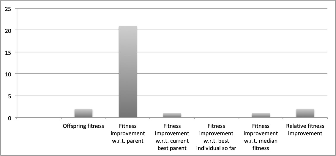
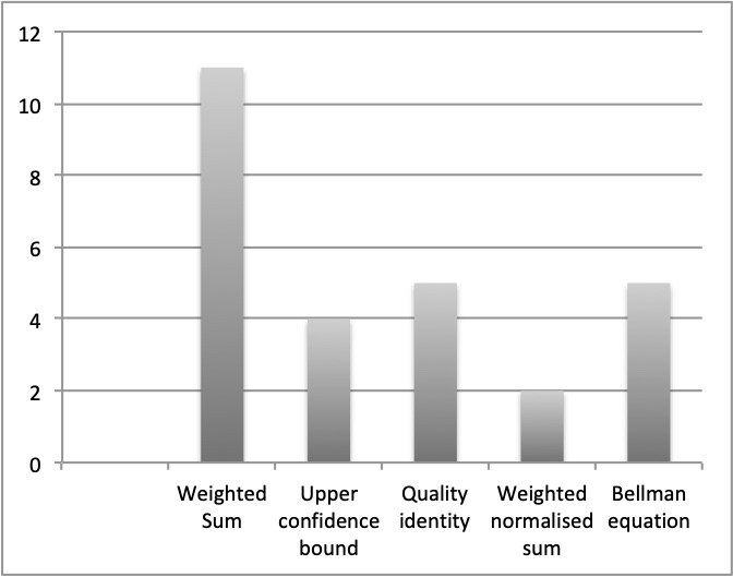
Selection choice	Probability choice

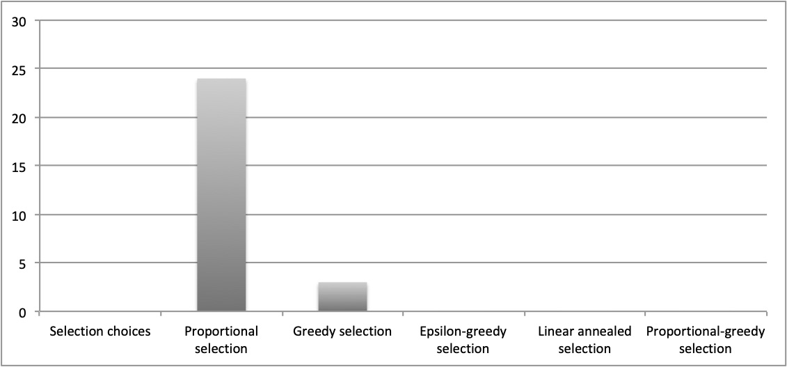
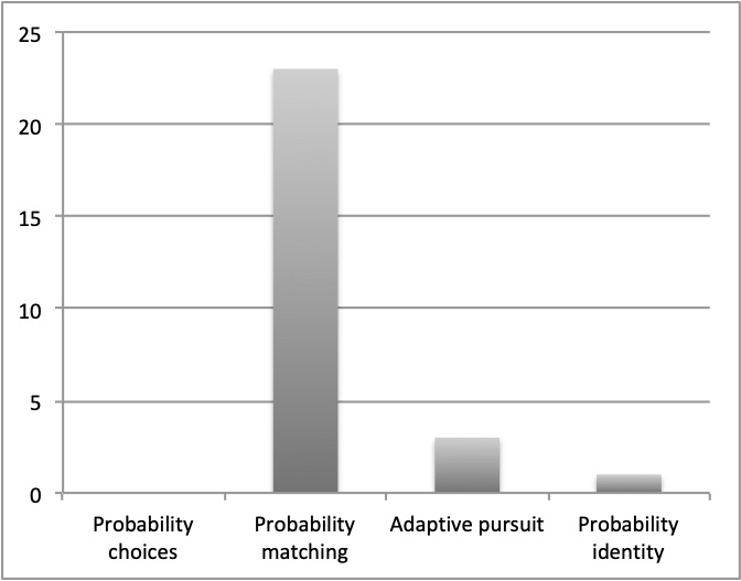
Reward metrics

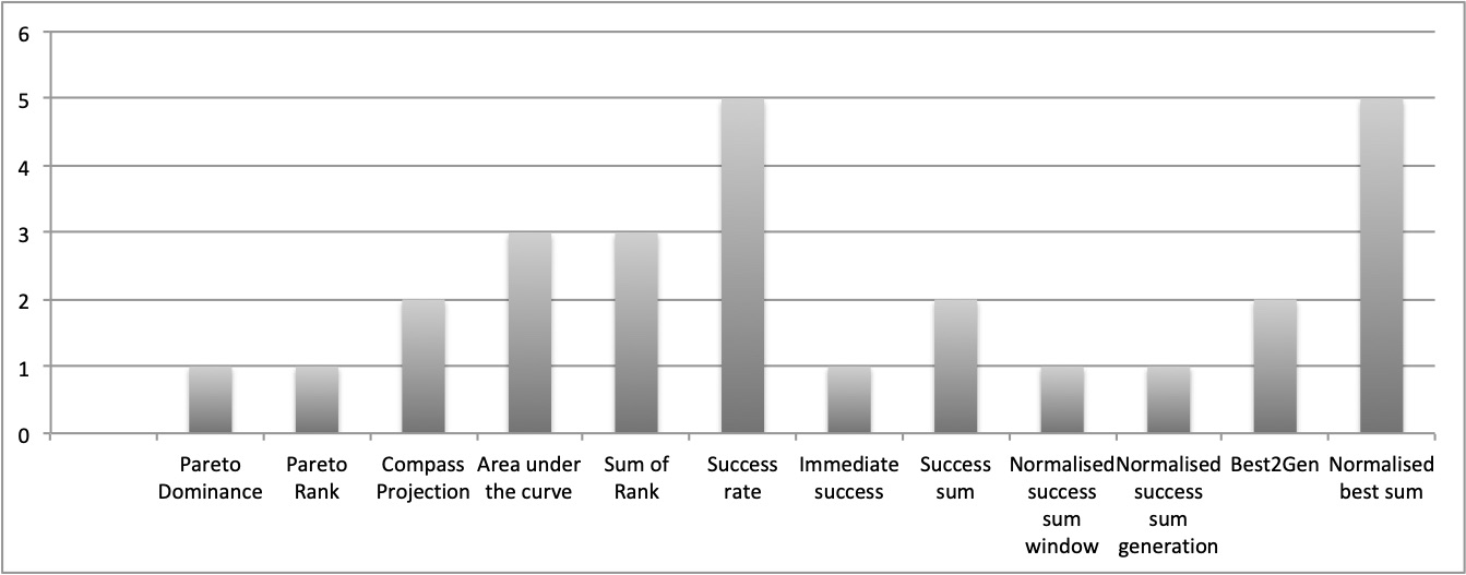
It can be clearly seen that a lot of emphasis is given on exploring novel reward choices among all components while proposing an AOS method. Success rate (eq. LABEL:SR1) and normalised best sum (eq. LABEL:B2) are among the popular choices for reward. In other components, Fitness improvement w.r.t. parent (eq. 2) is frequently used offspring metric and probability matching is a common choice by researchers that assign quality (eq. 22), probability (eq. 29) and selection mechanism (eq. 32). The combinations of these popular component choices have been explored in literature. [35] considers three reward definitions based on fitness improvement w.r.t. parent namely, pareto rank, pareto dominance and projection. To form a complete AOS method, these are combined with PM. Six combinations are tested in [37], area under the curve and sum of rank reward choices paired with dynamic multi-armed bandit (eq. 23 + eq. 29 + eq. 33), adaptive pursuit (eq. 22 + eq. 30 + eq. 32) and probability matching. We have not included statistical factor in the framework, and have only considered MAB instead of D-MAB. The papers testing other combinations include [16, 43, 14].

Besides these combinations, many other novel AOS methods can be designed using the framework. These combinations can be easily tested with differential evolution using the tool available on Github . The framework can be utilised to control the discrete parameters of not only DE but also any other evolutionary algorithm that has discrete parameters.

V Experimental Design

V-A Problem set

We use the bbob (Black-box optimisation benchmarking) [60] problem suite to train and test the proposed algorithms. bbob provides an easy to use tool-chain for benchmarking black-box optimisation algorithms for continuous domains and to compare the performance of numerical black-box optimisation algorithms. It consists of $24$ noiseless continuous benchmark functions [61] shown in table VII. Each function consists of $15$ different instances, totalling to $360$ function instances. An instance of a function is a rotation and/or translation of the original function leading to a different global optimum. These $24$ functions are grouped in five classes, namely, separable functions ($f01$ – $f05$), function with low or moderate conditioning ($f06$ – $f09$), functions with high conditioning and uni modal ($f10$ – $f14$), multi modal functions with adequate global structure ($f15$ – $f19$) and multi modal functions with weak global structure ($f20$ – $f24$).

Table VII: bbob function class and their functions

Class name	Function name
Separable functions	Sphere function ($f01$), Ellipsoidal Separable function ($f02$), Rastrigin Separable function ($f03$), Büche-Rastrigin function ($f04$), Linear Slope ($f05$)
Function with low or moderate conditioning	Attractive Sector function ($f06$), Step Ellipsoidal function ($f07$), Rosenbrock Original function ($f08$), Rosenbrock Rotated function ($f09$)
Functions with high conditioning and uni modal	Ellipsoidal non-Separable function ($f10$), Discus function ($f11$), Bent Cigar function ($f12$), Sharp Ridge function ($f13$), Different Powers function ($f14$)
Multi modal functions with adequate global structure	Rastrigin non-Separable function ($f15$), Weierstrass function ($f16$), Schaffers $f7$ function ($f17$), Schaffers $f7$ Moderately Ill-conditioned function ($f18$), Composite Griewank-Rosenbrock function $f8f2$ ($f19$)
Multi modal functions with weak global structure	Schwefel function ($f20$), Gallagher’s Gaussian $101$-me Peaks function ($f21$), Gallagher’s Gaussian 21-hi Peaks function ($f22$), Katsuura function ($f23$), Lunacek bi-Rastrigin function ($f24$)

V-B Parameter tuning

The framework consists of $6\times 12\times 5\times 3\times 5=5,400$ AOS methods. These methods have their own hyper-parameters which increase the number of unique combinations possible. As the parameter space is huge, we decided to combine the framework with an offline method that tunes the framework and returns a combination of choices for a problem set. We use the offline automatic configurator irace to tune the framework. irace is a racing algorithm that saves the hassle of manual tuning and allows for a fully specified and reproducible procedure. The input given to irace is the set of component choices along with the range of all hyper-parameters that needs tuning and a set of training function instances. In addition to tuning the framework and its hyper-parameters, it also tunes the parameters of the DE algorithm $F$, $NP$, $CR$ and $top_{NP}$. The parameter ranges/choices given to irace are shown in table VIII. The name, type (Real, Integer, categorical) and range of each parameter tuned by irace. The real-valued parameters take a two-point float value, integer type represents integer value in the given range and categorical can only select from the choices given. irace starts the tuning procedure by sampling a number of candidate parameter configurations from either a randomly initialised probability distribution or from a population of starting configurations given to it. The candidate configuration sampled by irace is an AOS method with a set of its hyper-parameter values and the DE parameters. The following steps are repeated until a budget given to irace is exhausted. The generated candidate configurations are evaluated on a sequence of problem instances. This process of evaluation on a sequence of instances is known as racing. During the racing process, poor performing candidate configurations are discarded and elite ones survive. A race terminates once the allocated computation budget is exhausted or the number of surviving candidate configurations is below some specific number. The best candidate configurations are then used to update the probability distribution. The distribution is biased towards good candidate configurations and is used to generate new candidate configurations for the next iteration.

Table VIII: Hyper-parameter choices given to irace

Parameter Name	Type	Range	Notes
DE parameters
F	Real	[0.1, 2.0]	Mutation Rate
CR	Real	[0.1, 1.0]	Crossover Rate
NP	Integer	[50, 400]	Population Size
$top_{NP}$	Real	[0.02, 1.0]	Top $p$ candidates
Component choices
Offspring Metric	Categorical	[0, 6]	Type of OM
Reward Type	Categorical	[0, 11]	Type of Reward
Quality Type	Categorical	[0, 4]	Type of Quality
Probability Type	Categorical	[0, 2]	Type of Probability
Selection Type	Categorical	[0, 4]	Type of Selection
Reward Choice parameters
$fix_{\text{appl}}$	Integer	[10, 50]	Fix number of applications
$\max_{\text{gen}}$	Integer	[1, 50]	Maximum number of generations
$\theta$	Categorical	(36, 45, 54, 90)	Projection angle
$\mathcal{W}$	Integer	(20, 150)	Size of window
$D$	Real	[0.0, 1.0]	Decay factor
$\gamma$	Categorical	(1, 2)	Success choice
$Frac$	Real	[0.0, 1.0]	Fraction of overall success
$\epsilon$	Real	[0.0, 1.0]	Noise
$\omega$	Categorical	(0, 1)	Normalisation choice
$C$	Real	[0.001, 1.0]	Scaling constant
$\alpha$	Categorical	(0, 1)	Decision parameter
$\beta$	Categorical	(0, 1)	Decision parameter
$\rho$	Categorical	(1, 2, 3)	Intensity
Quality Choice parameters
$\delta$	Real	(0.0, 1.0)	Decay rate
$C$	Real	(0.0, 1.0)	Scaling Factor
$q_{min}$	Real	(0.01, 1.0)	Minimum quality attained
$c_{1}$	Real	(0.0, 1.0)	Memory for current reward
$c_{2}$	Real	(0.0, 1.0)	Memory for previous reward
$\gamma$	Real	(0.01, 1.0)	Discount rate
Probability Choice parameters
$p_{\text{min}}$	Real	[0.0, 1.0]	Minimum selection probability
$\epsilon_{p}$	Real	(0.0, 1.0)	Noise
$\mu$	Real	(0.0, 1.0)	Learning rate
$p_{\text{max}}$	Real	(0.0, 1.0)	Maximum selection probability
Selection Choice parameters
$eps$	Real	[0.0, 1.0]	Random probability of selection

The budget given to irace is $10^{4}$ and the budget assigned to a DE run is $10^{4}\cdot n$ function evaluations where $n=20$ is the dimension of sampled function. All algorithms in this work focus on $n=20$ for all functions. We want to generalise on different classes of functions in the bbob noiseless functions of dimension $20$, thus we select function instances across different function classes. To prevent over-fitting, the training set contains two randomly selected function instances out of $15$ from each of the $24$ functions. Thus, training set consists of total $48$ out of $360$ function instances. These $48$ function instances are shown in table IX.

Table IX: Training set. $fxiy$ denotes a function instance $iy$ that is obtained by a transformation of original function $fx$.

Function class	Function instance
Separable functions	$f01i01$, $f01i07$, $f02i09$, $f02i15$, $f03i10$, $f03i05$, $f04i08$, $f04i06$, $f05i07$, $f05i01$
Function with low or moderate conditioning	$f06i13$, $f06i07$, $f07i02$, $f07i05$, $f08i06$, $f08i03$, $f09i10$, $f09i03$
Functions with high conditioning and uni modal	$f10i11$, $f10i04$, $f11i09$, $f11i02$, $f12i01$, $f12i03$, $f13i13$, $f13i12$, $f14i12$, $f14i11$
Multi modal functions with adequate global structure	$f15i07$, $f15i15$, $f16i02$, $f16i14$, $f17i12$, $f17i15$, $f18i09$, $f18i15$, $f19i01$, $f19i09$
Multi modal functions with weak global structure	$f20i10$, $f20i06$, $f21i05$, $f21i11$, $f22i01$, $f22i08$, $f23i03$, $f23i15$, $f24i08$, $f24i04$

As the parameter space given to irace is huge, we give four tuned AOS methods as the starting configurations to irace. Compass [15], PM-AdapSS [43], F-AUC-MAB [37] and RecPM-AOS [50] are among the popular AOS methods that act as initial population for irace to explore the parameter search space. Their hyper-parameters along with DE parameters are tuned using irace. The tuned AOS methods within DE are shown in table X. The first column shows the parameter name involved in the starting configurations followed by four AOS methods.

Table X: Starting configurations and the configuration returned by irace. The symbol ‘-’ in the table means that the parameter is not applicable to the AOS method.

Parameter name	RecPM-AOS	PM-AdapSS-NN	F-AUC-MAB	Compass	Configuration returned by irace (U-AOS-FW)
DE parameters
F	0.57	0.47	0.45	0.51	0.41
CR	0.93	0.96	0.21	0.95	0.91
NP	154	329	57	163	262
p in pbest	0.05	0.07	0.73	0.64	0.02
Component choices
Offspring Metric	2	2	2	2	2
Reward Type	LABEL:SR2	LABEL:W2	LABEL:R1	LABEL:DQ3	LABEL:SR2
Quality Type	26	22	23	24	26
Probability Type	29	29	29	29	29
Selection Type	32	32	33	32	32
Reward Choice hyper-parameters
$fix_{\text{appl}}$	-	-	-	66	-
$\theta$	-	-	-	90	-
$\mathcal{W}$	-	73	138	-	-
$D$	-	-	0.47	-	-
$\omega$	-	1	-	-	-
Quality Choice hyper-parameters
$\delta$	-	0.07	-	-	-
$c$	-	-	0.04	-	0.54
$c_{1}$	0.57	-	-	-	0.66
$c_{2}$	0.96	-	-	-	0.45
$\gamma$	0.43	-	-	-	-
Probability Choice hyper-parameters
$p_{\text{min}}$	0.08	0.06	0.02	0.08	0.04
$\epsilon_{p}$	0.26	0.53	0.72	0.55	0.22

VI Testing phase

After tuning, irace returns an AOS method along with its tuned hyper-parameter values and tuned DE parameter values given the starting configurations. The last column in table X shows the configuration returned by irace, abbreviated as U-AOS-FW. The returned configuration is a variant of RecPM-AOS [50] that acts as a starting configuration given to irace. RecPM-AOS assigns reward to an operator depending on the short term success of that operator and estimates quality based on the expected quality of possible selection of operators in the past. It shares similarities with PM-AdapSS AOS method, one of the starting configuration. PM-AdapSS utilises PM to select an operator whereas RecPM-AOS uses a variant of PM known as RecPM. Both AOS methods use reward based on the number of improvements from parent to offspring, however, PM-AdapSS uses average relative fitness improvement as immediate reward without using accumulated reward, whereas RecPM-AOS uses offspring survival rate as immediate reward combined with a fraction of its previous accumulated reward.

Algorithm 1 shows the working steps of AOS within DE in the testing phase. For a given test problem, this is simply the working of DE with multiple mutation operators where each parent is evolved using an operator selected with the selection method employed in the AOS method. Testing starts by initialising and evaluating the parent population. The OM values are calculated for each offspring to initialise the generation and window memory. The probability for each operator is initialised as $\frac{1}{K}$ where $K$ is the total number of mutation strategies. This gives every operator an equal chance to get selected in the beginning. Once the initialisation phase is over, the following steps are repeated until the stopping criteria are not satisfied. The parent population is evolved using a mutation strategy selected for each parent by selection definition in the AOS method. This improvement per parent is stored in OM. The memory is updated based on OM. The offspring population is evaluated and the solution among parent and offspring with better fitness survives. This is followed by reward, quality and probability update according to the AOS method. The selection of operator is performed based on the probability of each operator. Once the algorithm terminates, best fitness value is returned.

Algorithm 1 AOS method formed with the component choices from the framework coupled with DE

1:  Given: Tuned $CR$, $F$ and $NP$; Component choices from AOS framework

2:  Initialise and evaluate fitness of each individual $x_{i}$ in the population

3:  $g=0$ (generation number)

4:  Calculate $\textit{OM}(0,k,op)$, $\forall$ k

5:  Initialise generation and window memory using $\textit{OM}(0,k,op)$, $\forall$ k

6:  Initialise probability $P_{0,op}$, $\forall\textit{op}\in\textit{Op}$

7:  while stopping condition is not satisfied do

8:     for each $x_{i}$, $i=1,\dotsc,NP$ do

9:        if one or more operators not yet applied then

10:           $\textit{op}=\text{Uniform selection among operator(s) not yet applied}$

11:        else

12:           $\textit{op}=\text{Select a mutation strategy based on the selection choice}$

13:        Generate offspring using selected operator op

14:     Calculate $\textit{OM}(g,k,op)$

15:     Update generation and window memory using $\textit{OM}(g,k,op)$, $\forall$ k

16:     Evaluate offspring population

17:     Perform survival selection

18:     Calculate reward for each operator $R_{g+1,op}$

19:     Estimate quality for each operator $Q_{g+1,op}$

20:     Update probability for each operator $P_{g+1,op}$

21:     $g=g+1$

We select four tuned AOS methods within DE PM-AdapSS [43], F-AUC-MAB [37], Compass [15] and RecPM-AOS [50]; two non-AOS DE algorithms with one mutation strategy, JaDE [62] and R-SHADE [63] to compare with the returned configuration. PM-AdapSS and F-AUC-MAB were introduced in the context of selecting a mutation strategy in DE [20]. In particular, PM-AdapSS uses probability matching as the method for operator selection, whereas F-AUC-MAB employs a method inspired by multi-armed bandits. Compass evaluates an operator’s impact using two measures, mean fitness and population fitness diversity. It measures how well the operator balances the exploration and exploitation. The two non-AOS algorithms employ different ways to self-adapt crossover and mutation rate in DE. JaDE is a DE variant that adapts the crossover probability $CR$ and mutation factor $F$ using the values which proved to be useful in the current generation. R-SHADE is an improvement upon JaDE which employs a restart mechanism and uses a parameter adaptation mechanism based on a historical record of successful parameter settings to adapt $CR$ and $F$. JaDE and R-SHADE utilise same mutation strategy “current-to-pbest” to evolve population and it is one of the operators adapted by U-AOS-FW and other AOS methods in comparison.

The data for non-AOS methods is taken from the coco website. The returned configuration and other six algorithms from the literature are evaluated on the remaining $312$ bbob noiseless benchmark set on dimension $20$. We use plots of the Empirical Cumulative Distribution Function (ECDF) to assess their performance (Fig. 6). The ECDF displays the proportion of problems solved within a specified budget of function evaluations (FEvals) for different targets $f_{\text{target}}=f_{\mathrm{opt}}+\Delta f$, where $f_{\mathrm{opt}}$ is an the optimum function value to reach with some precision $\Delta f\in[10^{-8},10^{2}]$. In the plots, FEvals is given on the x-axis and y-axis represents the fraction of problems solved. A large symbol ‘$\times$’ shows the maximum number of function evaluations (budget) given to each algorithm. We give ${10}^{5}\cdot 20$ FEvals as the budget to each algorithm with AOS method. The results reported after this symbol use bootstrapping to estimate the number of evaluations to reach a specific target for a problem [64]. The results denoted with best 2009 correspond to the artificial best algorithm from the bbob-2009 workshop constructed from the data of the algorithm with the smallest $\mathrm{aRT}$ (average Run Time) for each set of problems with the same function, dimension and target. The $\mathrm{aRT}$ is calculated as the ratio of the number of function evaluations for reaching the target value over successful runs (or trials), plus the maximum number of evaluations for unsuccessful runs, divided by the number of successful trials. The trials that reached $f_{\text{target}}$ within the specified budget are termed as successful trials, $\#succ$. The $\mathrm{aRT}$ tables for eight algorithms are shown in tables XI and XII.

VII Experiments and Results

During the tuning phase, irace samples parameters from their individual parameter distribution. This distribution is updated to focus on the efficient parameter range. The frequency of sampled frequency of the parameters is shown in figure 5. Categorical parameters that take values from a set of values are shown in the figure such as OM_choice and frac. Parameters that take floating-values such as $FF$ and decay sample from a probability distribution such as a normal distribution.

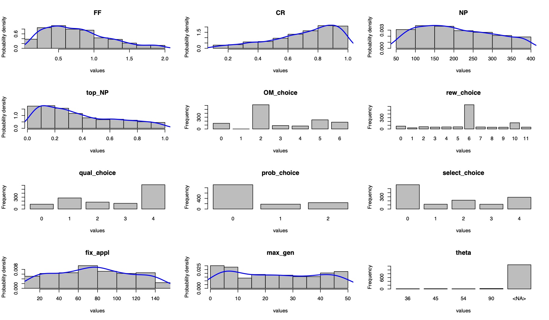
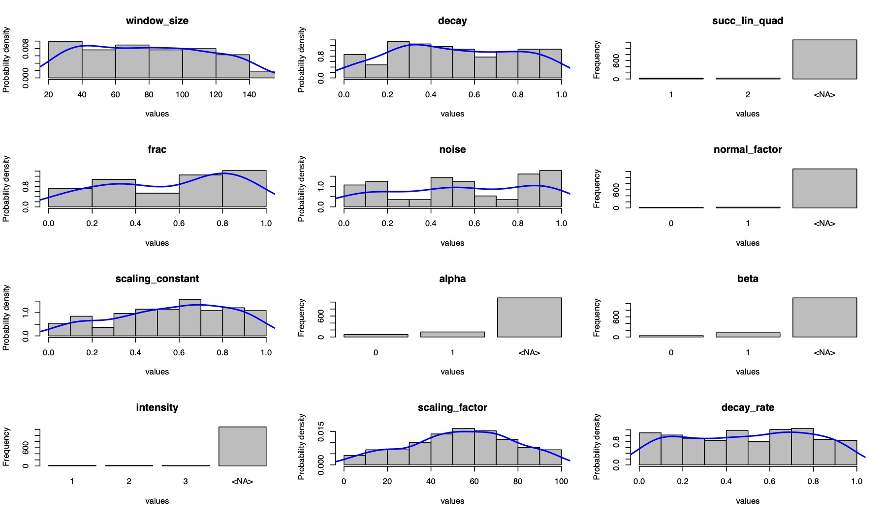
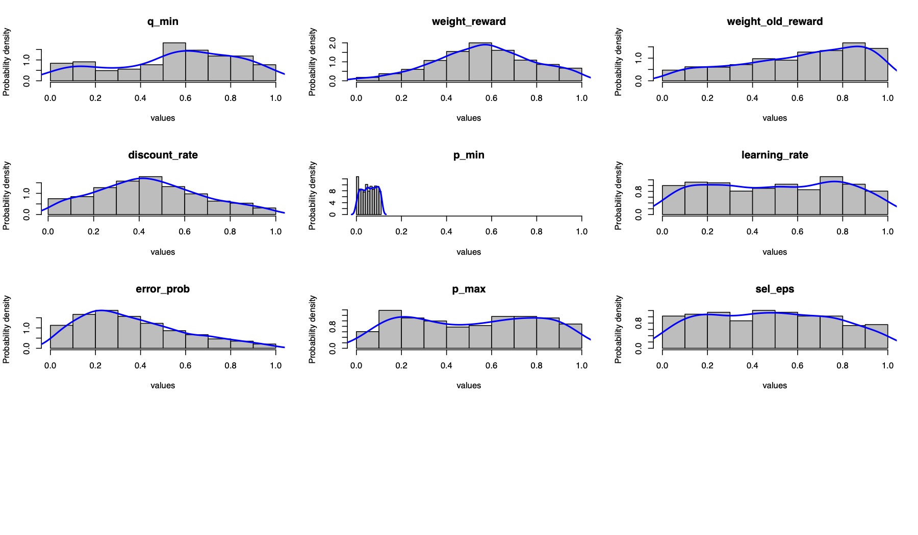
Figure 5: Parameter sampling frequency. FF for F, top_NP for p in pbest, $\theta$ for theta, $\mathcal{W}$for window, D for decay, $\gamma$ for succ_lin_quad, Frac for frac, $\epsilon$ for noise, $\omega$ for normal_factor, C for scaling_constant, $\alpha$ for alpha, $\beta$ for beta, $\rho$ for intensity, c for scaling_factor, $\delta$ for decay_rate, c1 for weight_reward, c2 for weight_old_reward, $\gamma$ for discount_rate, $\mu$ for learning_rate, $\epsilon_{p}$ for error_prob, eps for sel_eps

VII-A Comparison of U-AOS-FW with other tuned AOS methods

ECDF graphs on 24 functions each with 13 test instances are shown in figure 6. It also shows class-wise and overall performance on the test set. These graphs clearly show that the configuration returned by irace, U-AOS-FW reaches all targets with competitive speed for functions f001, f002 and f005-f014 in comparison with RecPM-AOS, PM-AdapSS, Compass and F-AUC-MAB. Looking at the separable class Compass and U-AOS-FW solves problems with the same speed solving the same number of problems as PM-AdapSS. Although U-AOS-FW is a variant of RecPM-AOS, the former solves more problems than the latter with faster speed. F-AUC-MAB has shown exceptional performance in terms of speed and problems solves compared to other AOS methods for separable class of problems. U-AOS-FW performed best for low/moderate conditioning problems reaching all targets for all 4$\times$13 test instances falling under this category and the same performance of all AOS methods can be seen in the case of high conditioning class of problems. F-AUC-MAB performed worse on low/moderate and high conditioning class, solving the least number of problems. U-AOS-FW and RecPM-AOS excelled in the multi model (adequate structure) class of problems. They showed similar performance with former solving faster than any other algorithm. U-AOS-FW came second in the multi model (weak structure) problems after F-AUC-MAB which solved more than 30% problems. Overall, U-AOS-FW solved approximately 65% of total problems which is more than the number of problems solved by any tuned AOS method and also with faster speed compared to any AOS method.

Figure 6: ECDFs on test set. F-AUC for F-AUC-MAB, UFW for U-AOS-FW, RecPM for RecPM-AOS, AdapSS for PM-AdapSS

f001	f002
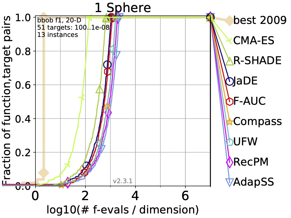
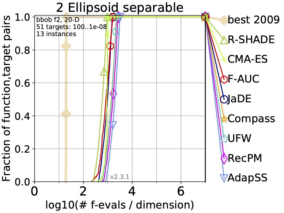
f003	f004
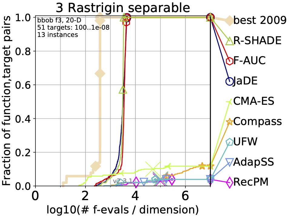
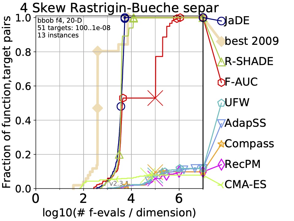
f005	f006

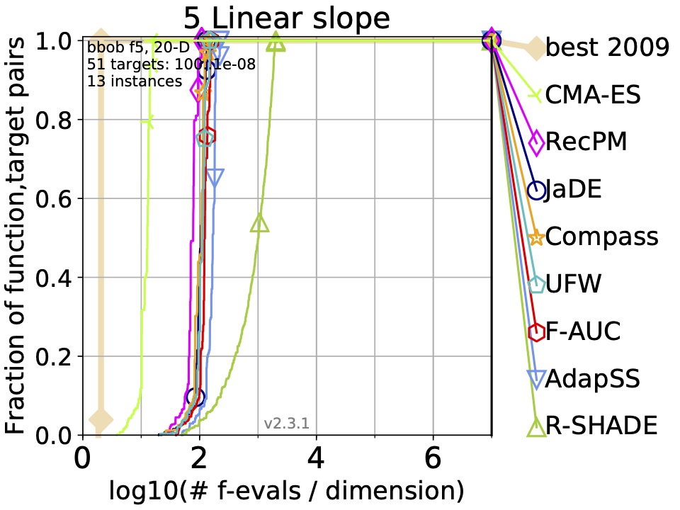
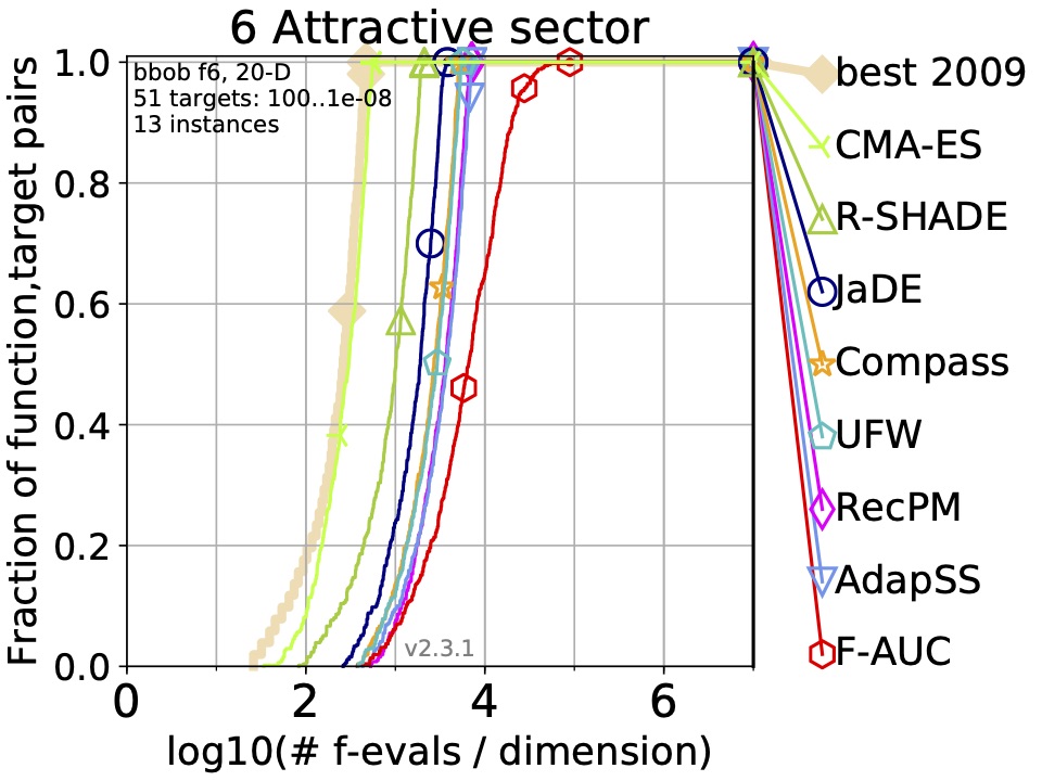
Figure 7: ECDFs on test set. F-AUC for F-AUC-MAB, UFW for U-AOS-FW, RecPM for RecPM-AOS, AdapSS for PM-AdapSS

f007	f008
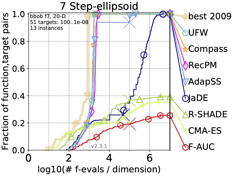
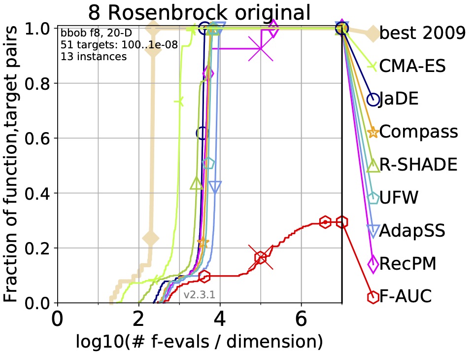
f009	f010
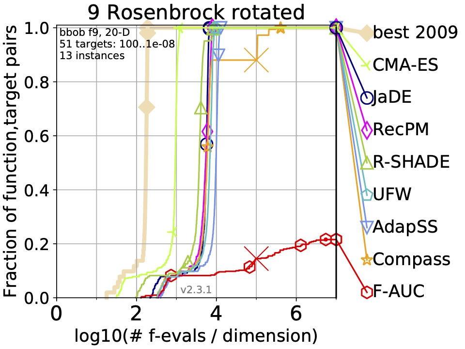
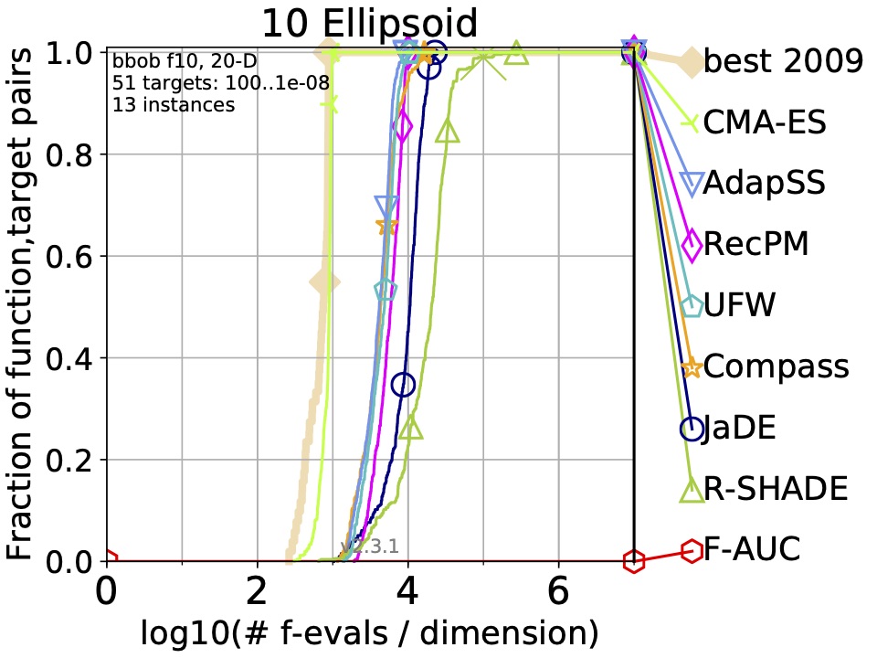
f011	f012

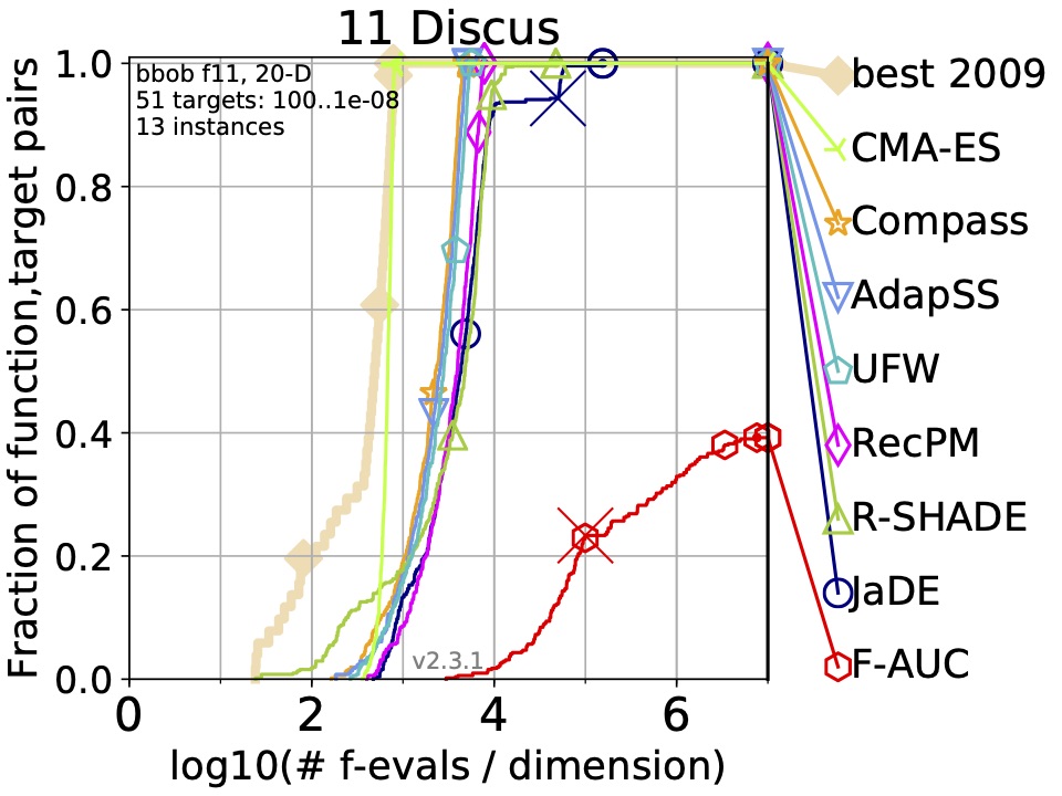
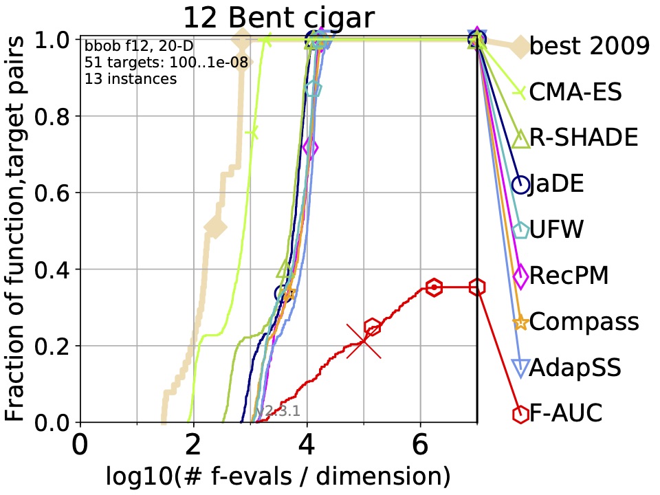
Figure 8: ECDFs on test set. F-AUC for F-AUC-MAB, UFW for U-AOS-FW, RecPM for RecPM-AOS, AdapSS for PM-AdapSS

f013	f014
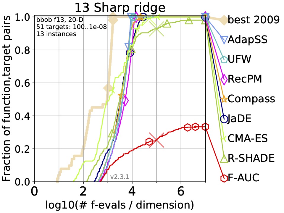
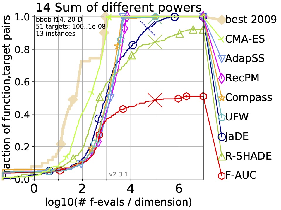
f015	f016
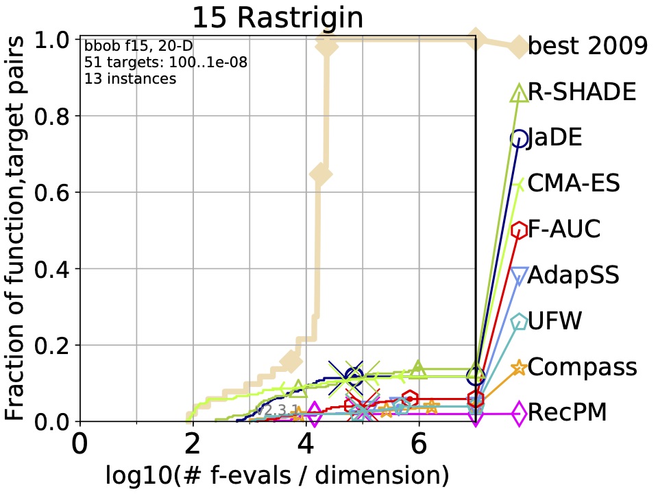
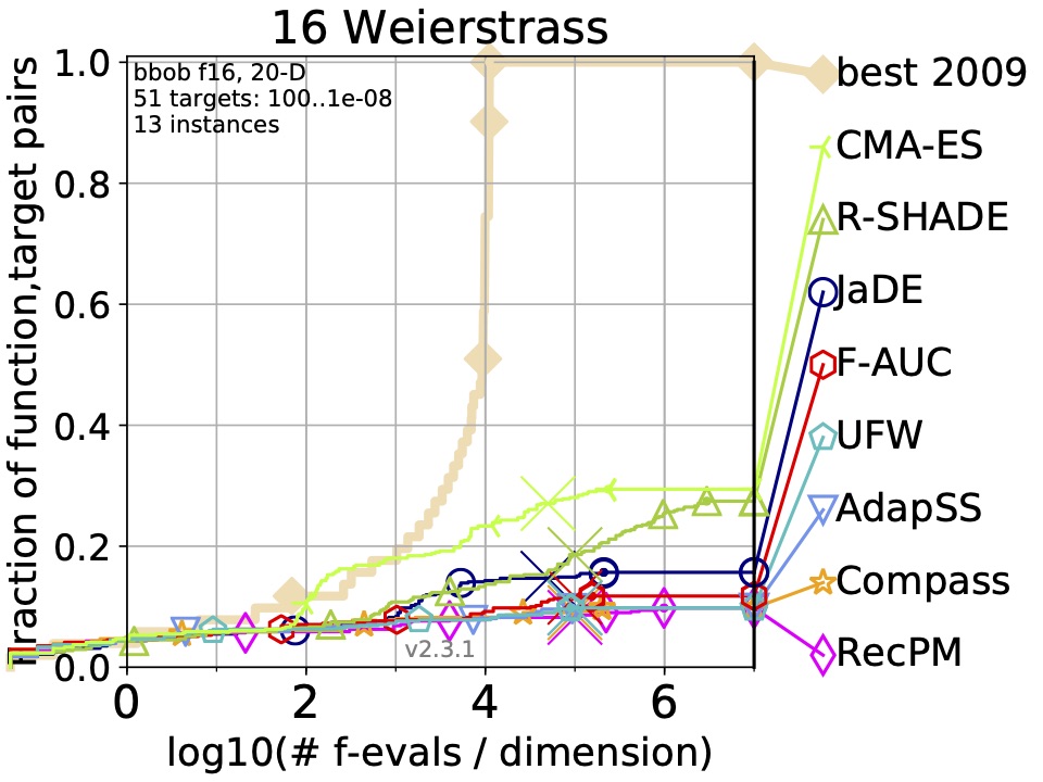
f017	f018

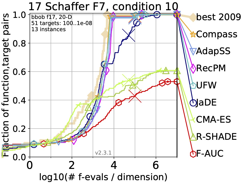
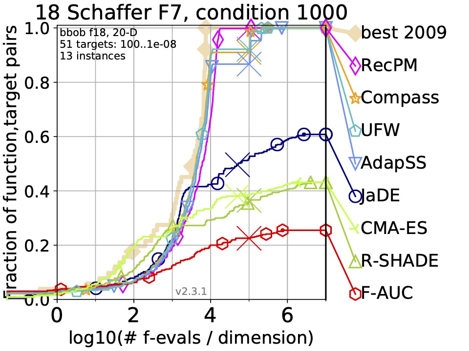
Figure 9: ECDFs on test set. F-AUC for F-AUC-MAB, UFW for U-AOS-FW, RecPM for RecPM-AOS, AdapSS for PM-AdapSS

f019	f020
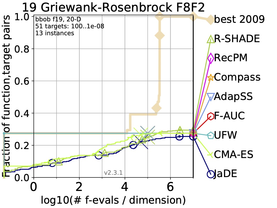
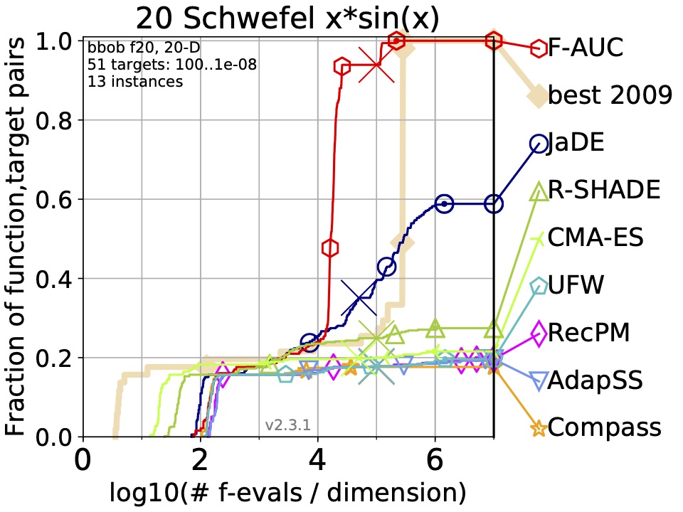
f021	f022
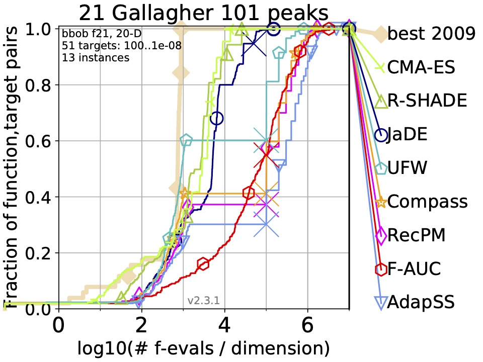
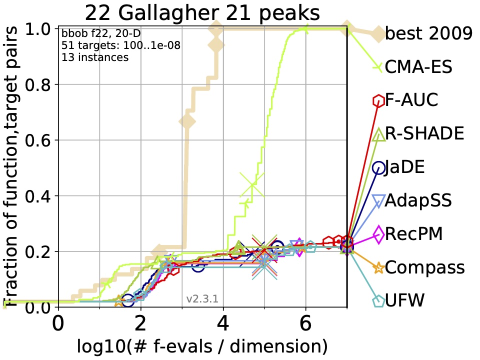
f023	f024

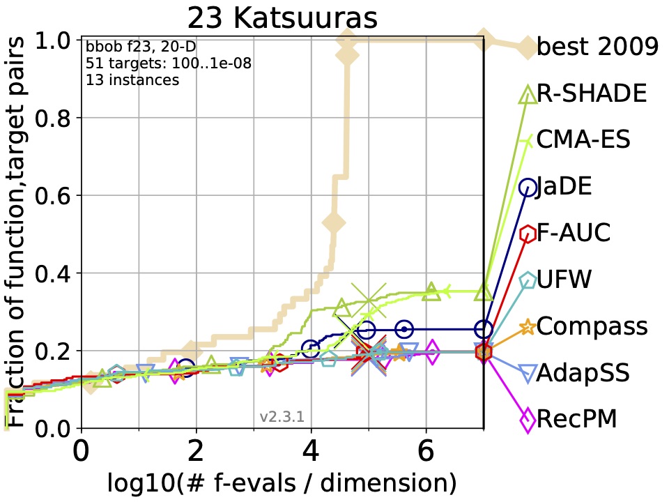
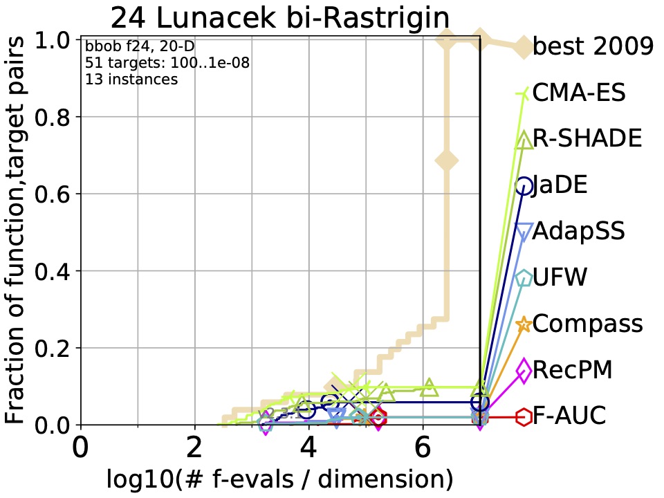
Figure 10: ECDFs on test set. F-AUC for F-AUC-MAB, UFW for U-AOS-FW, RecPM for RecPM-AOS, AdapSS for PM-AdapSS

Separable	Low/moderate conditioning
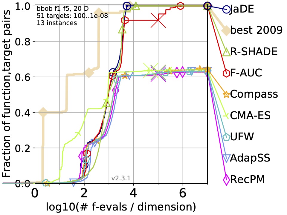
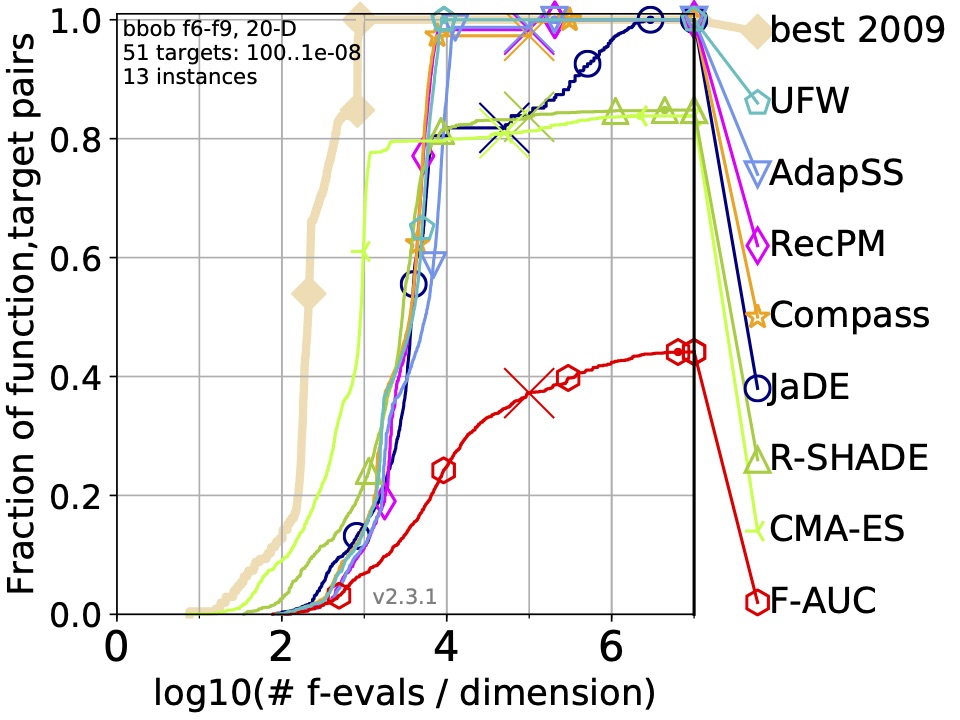
High conditioning	multi modal (adequate structure)
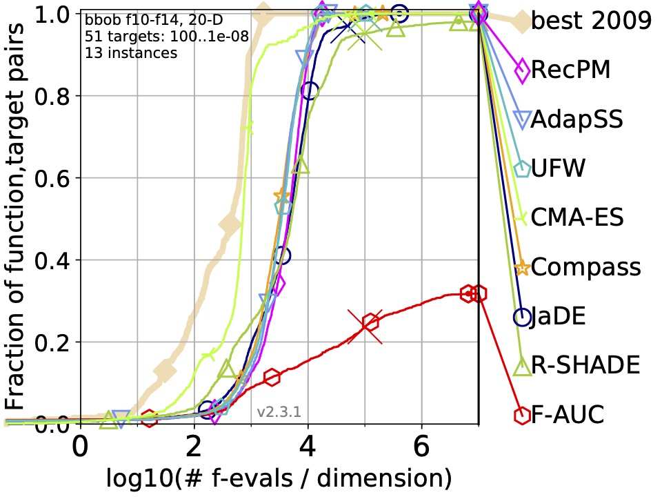
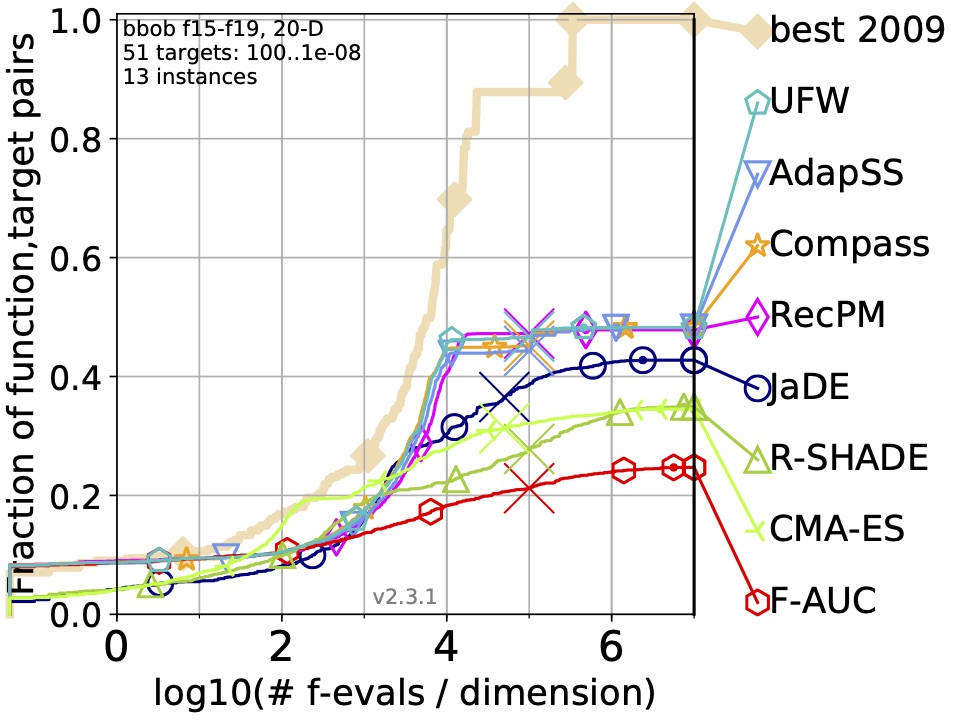
multi modal (weak structure)	Overall

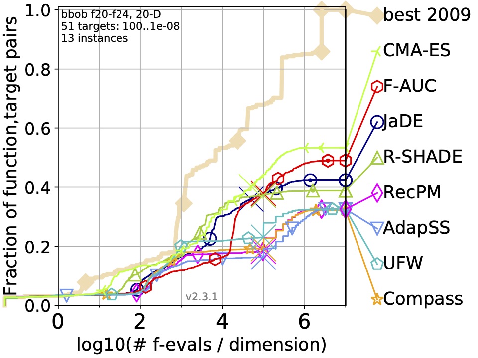
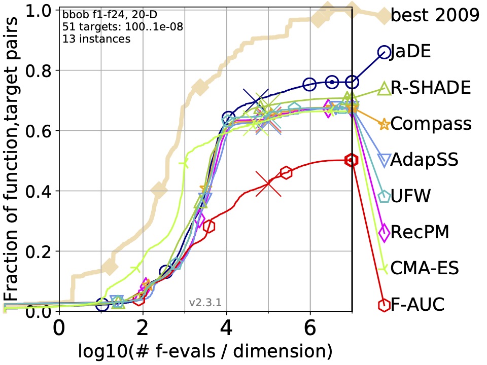
VII-B Comparison of U-AOS-FW with non-AOS methods

We compare the performance of U-AOS-FW with non-AOS methods that is JaDE and R-SHADE. The latter two are variants of DE utilising one strategy to evolve population of candidate solutions. U-AOS-FW outperformed the two algorithms in three classes namely multi model (adequate structure), low/moderate and high conditioning problems. It excelled not only in solving maximum number of problems in these three class but also with higher speed. Overall, U-AOS-FW is ranked third after JaDE and R-SHADE in solving a number of problems.

VII-C Comparison of U-AOS-FW trained on nine operators with RecPM-AOS on four operators

We are interested in analysing whether adding new operators in the set of operators for AOS method to choose from lead to any improvement in performance. Thus, we made an attempt in analysing the difference in performance of U-AOS-FW trained on nine operators to RecPM-AOS trained on four operators (RecPM1). To analyse this, we compare the class-wise ECDF graphs of U-AOS-FW shown in figure 10 and RecPM-AOS from paper [50]. There does not seem be any difference in performance of U-AOS-FW and RecPM1 in solving separable, multi modal (adequate), low and high conditioning class problems, that is they solve the same number of problems. However, U-AOS-FW solves the function instances of low/moderate conditioning and multi modal (adequate structure) with greater speed. In solving multi modal (weak structure), U-AOS-FW outperforms RecPM1 in terms of speed and different targets. Thus, adding more operators helped solving more problems with higher speed, showing a better arrangement for exploration and exploitation of search space.

Next we try to identify the operators that lead to differences in performance of these two algorithms. Thus, further to analysing ECDF graphs we plan to better understand the impact of the selected operators by comparing the graphs generated as a result of running algorithms. We compare the performance of RecPM1 from paper [50] (figure 11) and by U-AOS-FW (figure 15) on functions $f05$ and $f07$ each with instance $i01$. These function instances are selected at random among the test instances of functions. Figure 11 is a result of four operator applications by RecPM1 and figure 15 is a result of utilising nine different operators by U-AOS-FW in different generations. A value of $p_{\text{min}}$= $0.17$ and $0.04$ controls the level of adaptation of operators in algorithms RecPM1 and U-AOS-FW respectively. To distinguish the operators, we represent them with different colors. The operators utilised by different candidate solutions to produce offspring in a generation are represented by a bar, all raising to the same level. For RecPM1 and U-AOS-FW, population size is $168$ and $262$ respectively. The second figure for a function instance shows the best fitness seen as the generation progresses. To show the operator applications from each class, we have included the operator selections and best fitness progress for function instances $f04i02$, $f08i10$, $f13i04$, $f17i02$ and $f23i04$, shown in figure 15.

Figure 11: Operator application and best fitness graphs for DE-RecPM-AOS. Op1: “rand/1”, Op2: “rand/2”, Op3: “rand-to-best/2”, Op4: “current-to-rand/1”

$f05i01$
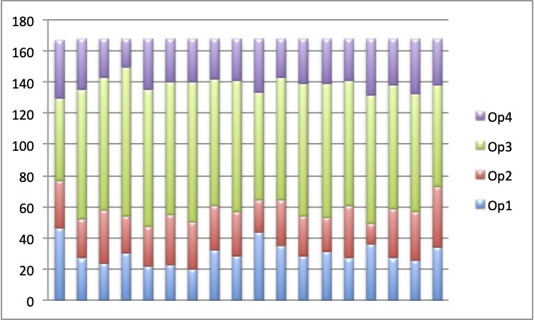
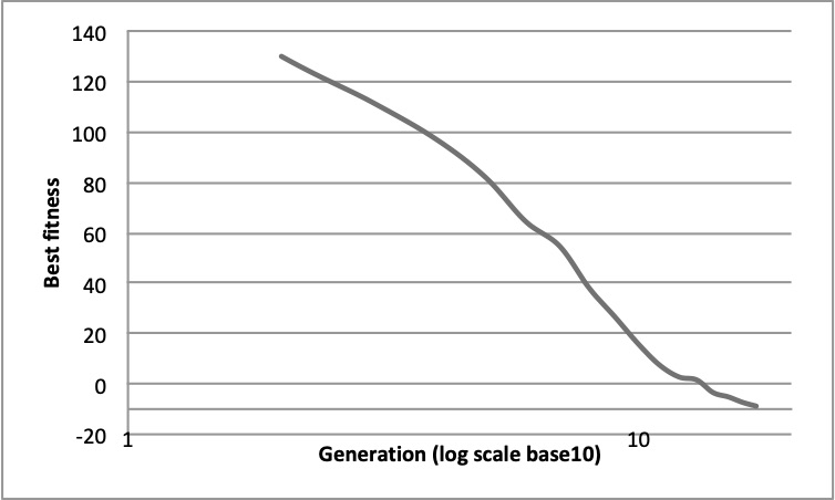
$f07i01$

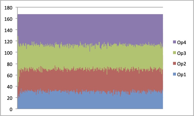
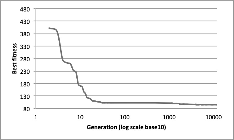
Figure 12: Operator application and best fitness graphs for U-AOS-FW. Op1: “rand/2”, Op2: “best/1”, Op3: “current-to-best/1”, Op4: “best/2”, Op5: “rand/1”, Op6: “rand-to-best/2”, Op7: “curr-to-rand/1”, op8: “curr-to-pbest/1”, Op9: “curr-to-pbest/1(archived)”

$f05i01$
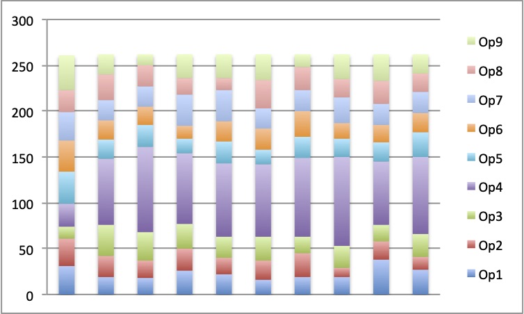
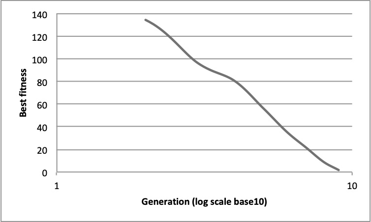
$f07i01$

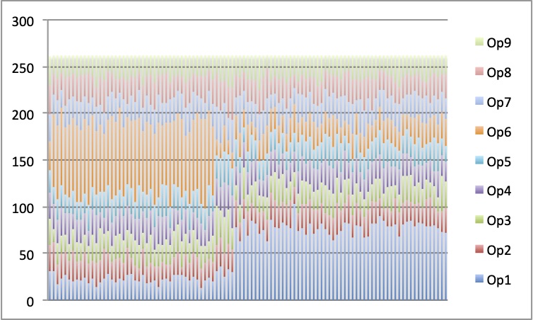
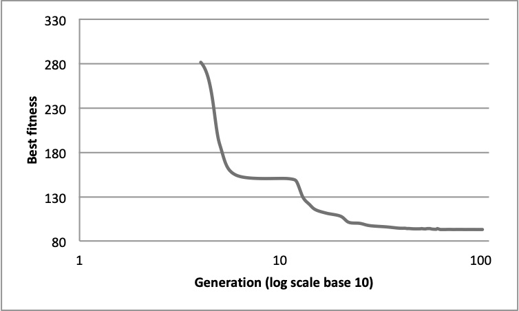
Figure 13: Operator application and best fitness graphs for U-AOS-FW. Op1: “rand/2”, Op2: “best/1”, Op3: “current-to-best/1”, Op4: “best/2”, Op5: “rand/1”, Op6: “rand-to-best/2”, Op7: “curr-to-rand/1”, op8: “curr-to-pbest/1”, Op9: “curr-to-pbest/1(archived)”

$f04i02$
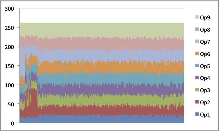
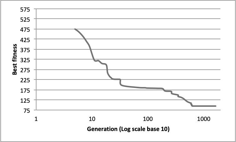
$f08i10$

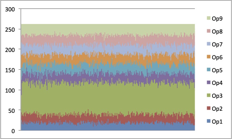
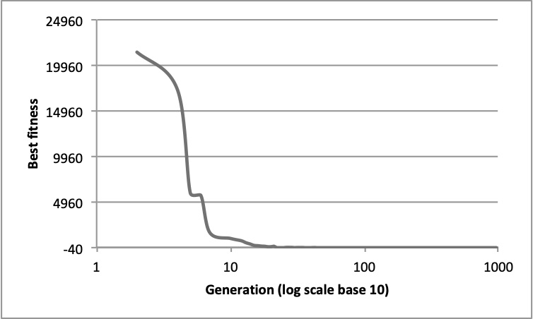
Figure 14: Operator application and best fitness graphs for U-AOS-FW. Op1: “rand/2”, Op2: “best/1”, Op3: “current-to-best/1”, Op4: “best/2”, Op5: “rand/1”, Op6: “rand-to-best/2”, Op7: “curr-to-rand/1”, op8: “curr-to-pbest/1”, Op9: “curr-to-pbest/1(archived)”

$f13i14$
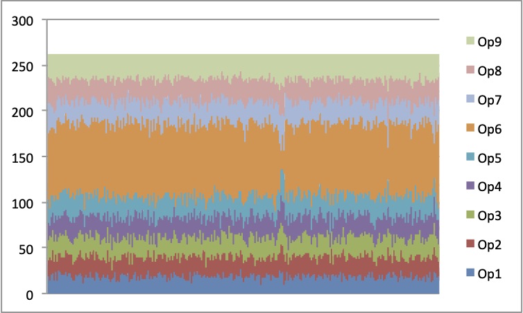
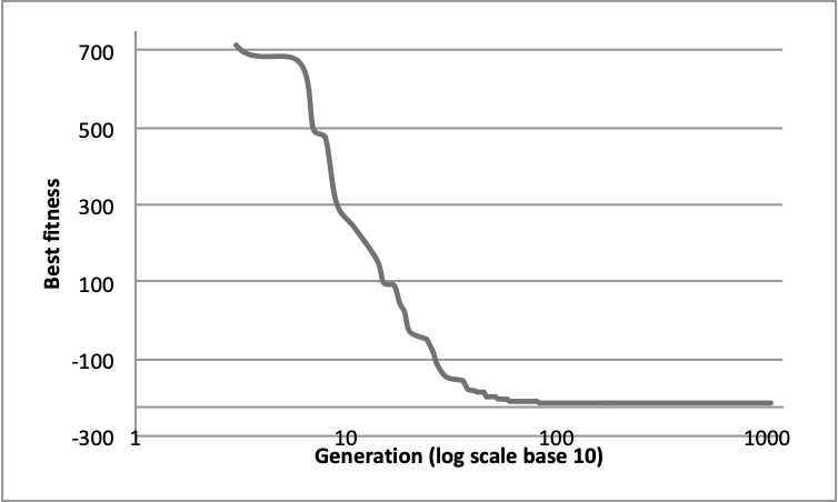
$f17i02$

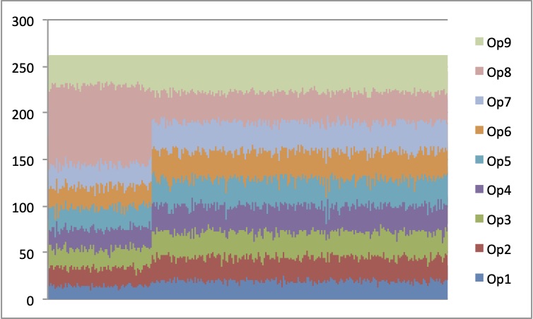
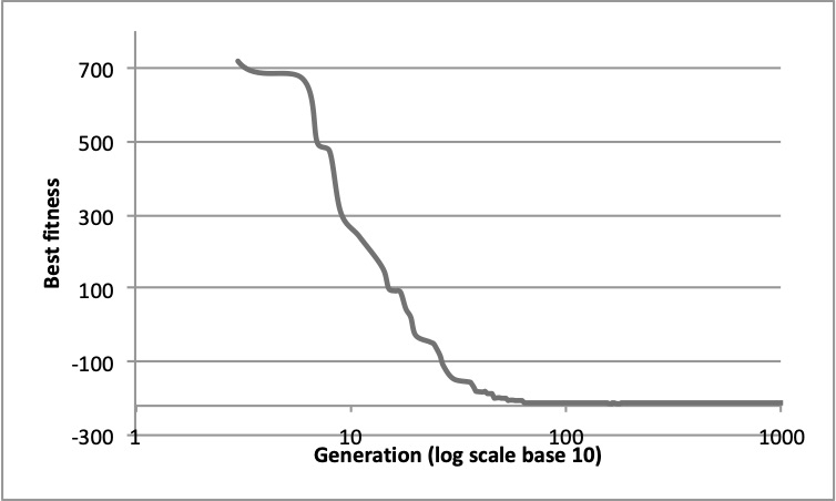
Figure 15: Operator application and best fitness graphs for U-AOS-FW. Op1: “rand/2”, Op2: “best/1”, Op3: “current-to-best/1”, Op4: “best/2”, Op5: “rand/1”, Op6: “rand-to-best/2”, Op7: “curr-to-rand/1”, op8: “curr-to-pbest/1”, Op9: “curr-to-pbest/1(archived)”

$f23i04$

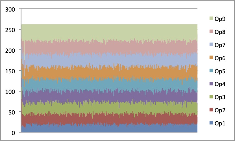
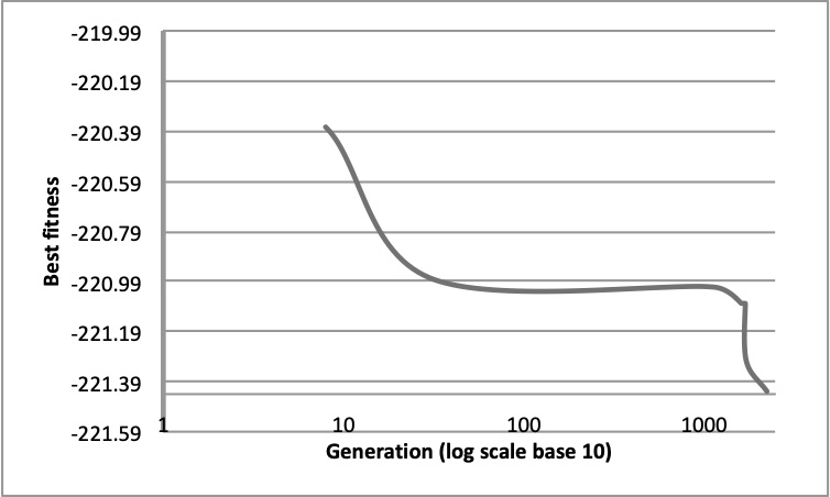
Table XI: Average runtime $\mathrm{aRT}$

$\Delta f_{\mathrm{opt}}$ 1e1 1e0 1e-1 1e-2 1e-3 1e-5 1e-7 #succ f1 43 43 43 43 43 43 43 15 /15 U-AOS-FW 73 (11) 141 (8) 217 (11) 294 (17) 368 (18) 527 (21) 670 (35) 13 /13 R-SHADE 28 (7)^⋆3 61 (10)^⋆3 91 (11)^⋆3 122 (14)^⋆3 152 (13)^⋆3 211 (17)^⋆3 269 (11)^⋆3 13 /13 RecPM-AOS 86 (16) 169 (14) 255 (29) 345 (15) 434 (37) 611 (38) 790 (56) 13 /13 PM-AdapSS 92 (14) 192 (16) 297 (14) 400 (27) 507 (16) 710 (17) 926 (16) 13 /13 F-AUC-MAB 58 (7) 113 (6) 164 (9) 219 (16) 270 (32) 376 (24) 480 (45) 13 /13 Compass 67 (9) 141 (10) 217 (12) 291 (17) 368 (10) 517 (12) 667 (13) 13 /13 JaDE 48 (10) 94 (9) 144 (10) 193 (8) 241 (9) 341 (10) 438 (12) 13 /13 f2 385 386 387 388 390 391 393 15 /15 U-AOS-FW 40 (3) 48 (2) 57 (4) 66 (4) 74 (5) 91 (5) 107 (5) 13 /13 R-SHADE 18 (2) 21 (2) 24 (2) 28 (2) 31 (2) 37 (3) 43 (3) 13 /13 RecPM-AOS 45 (5) 55 (4) 65 (3) 74 (5) 83 (4) 103 (6) 122 (6) 13 /13 PM-AdapSS 55 (3) 67 (0.9) 78 (3) 90 (3) 101 (3) 124 (2) 147 (2) 13 /13 F-AUC-MAB 24 (2) 30 (2) 35 (7) 40 (7) 46 (5) 56 (15) 67 (8) 13 /13 Compass 39 (1) 47 (2) 55 (2) 64 (2) 71 (2) 88 (2) 104 (2) 13 /13 JaDE 28 (1) 33 (1) 39 (2) 44 (2) 49 (2) 61 (3) 71 (3) 13 /13 f3 5066 7626 7635 7637 7643 7646 7651 15 /15 U-AOS-FW $\infty$ $\infty$ $\infty$ $\infty$ $\infty$ $\infty$ $\infty$ 2e6 0 /13 R-SHADE 7 .6(0.5) 7 .1(0.3) 7 .6(0.3) 7 .9(0.2) 8 .1(0.2) 8 .4(0.2)^⋆3 8 .7(0.3)^⋆3 13 /13 RecPM-AOS $\infty$ $\infty$ $\infty$ $\infty$ $\infty$ $\infty$ $\infty$ 2e6 0 /13 PM-AdapSS $\infty$ $\infty$ $\infty$ $\infty$ $\infty$ $\infty$ $\infty$ 2e6 0 /13 F-AUC-MAB 11 (0.8) 8 .4(0.9) 8 .7(0.4) 9 .0(0.8) 9 .3(0.6) 10 (1) 11 (1) 13 /13 Compass 5069 (4441) $\infty$ $\infty$ $\infty$ $\infty$ $\infty$ $\infty$ 2e6 0 /13 JaDE 6 .4(0.3)^⋆3 6 .0(0.2)^⋆3 6 .8(0.2)^⋆3 7 .6(0.2)^⋆ 8 .3(0.1) 10 (0.1) 11 (0.1) 13 /13 f4 4722 7628 7666 7686 7700 7758 1.4e5 9 /15 U-AOS-FW 2563 (3709) $\infty$ $\infty$ $\infty$ $\infty$ $\infty$ $\infty$ 2e6 0 /13 R-SHADE 9 .5(0.8) 8 .3(0.4) 11 (5) 12 (0.4) 12 (11) 12 (11) 0 .70(0.3) 13 /13 RecPM-AOS $\infty$ $\infty$ $\infty$ $\infty$ $\infty$ $\infty$ $\infty$ 2e6 0 /13 PM-AdapSS 5416 (3812) $\infty$ $\infty$ $\infty$ $\infty$ $\infty$ $\infty$ 2e6 0 /13 F-AUC-MAB 12 (2) 125 (0.7) 313 (587) 313 (520) 312 (260) 311 (451) 17 (25) 6 /13 Compass $\infty$ $\infty$ $\infty$ $\infty$ $\infty$ $\infty$ $\infty$ 2e6 0 /13 JaDE 8 .1(0.3)^⋆2 7 .0(0.1)^⋆3 8 .0(0.2)^⋆3 8 .9(0.2) 10 (0.1) 11 (0.2) 0 .71(9e-3) 13 /13 f5 41 41 41 41 41 41 41 15 /15 U-AOS-FW 47 (8) 55 (7) 56 (12) 57 (7) 57 (9) 57 (9) 57 (11) 13 /13 R-SHADE 114 (11) 210 (19) 307 (25) 399 (30) 488 (19) 676 (34) 860 (45) 13 /13 RecPM-AOS 33 (4) 37 (8) 39 (7)^⋆2 39 (9)^⋆2 39 (7)^⋆2 39 (9)^⋆2 39 (8)^⋆2 13 /13 PM-AdapSS 69 (9) 83 (11) 85 (10) 85 (8) 85 (22) 85 (13) 85 (6) 13 /13 F-AUC-MAB 49 (3) 59 (9) 62 (11) 63 (10) 63 (8) 63 (8) 63 (7) 13 /13 Compass 42 (7) 50 (6) 51 (12) 51 (11) 51 (7) 51 (10) 51 (7) 13 /13 JaDE 42 (6) 52 (8) 53 (7) 53 (3) 53 (5) 53 (6) 53 (7) 13 /13 f6 1296 2343 3413 4255 5220 6728 8409 15 /15 U-AOS-FW 14 (2) 12 (1) 11 (0.6) 11 (1) 11 (1.0) 11 (0.5) 12 (0.3) 13 /13 R-SHADE 4 .1(0.5)^⋆3 3 .9(0.4)^⋆3 3 .8(0.5)^⋆3 3 .9(0.3)^⋆3 3 .9(0.5)^⋆3 4 .0(0.4)^⋆3 4 .1(0.4)^⋆3 13 /13 RecPM-AOS 19 (2) 15 (2) 14 (1) 14 (1) 14 (0.9) 14 (0.9) 14 (0.8) 13 /13 PM-AdapSS 18 (2) 15 (1) 14 (0.9) 14 (0.6) 14 (0.4) 15 (0.4) 15 (0.2) 13 /13 F-AUC-MAB 23 (4) 23 (5) 23 (9) 26 (8) 29 (15) 39 (24) 53 (33) 13 /13 Compass 14 (1) 11 (0.8) 10 (0.7) 11 (0.5) 10 (0.5) 11 (0.4) 11 (0.1) 13 /13 JaDE 9 .4(0.8) 7 .8(0.6) 7 .3(0.8) 7 .3(0.9) 7 .2(0.9) 7 .4(0.4) 7 .4(0.6) 13 /13 f7 1351 4274 9503 16523 16524 16524 16969 15 /15 U-AOS-FW 5 .2(0.6) 3 .7(0.6) 2 .3(0.2) 1 .9(0.1) 1 .9(0.1) 1 .9(0.2) 1 .9(0.2) 13 /13 R-SHADE 2 .1(0.3)^⋆3 33 (19) 76 (87) $\infty$ $\infty$ $\infty$ $\infty$ 2e6 0 /13 RecPM-AOS 6 .5(1.0) 4 .6(0.6) 3 .0(0.3) 2 .5(0.3) 2 .5(0.3) 2 .5(0.4) 2 .6(0.4) 13 /13 PM-AdapSS 6 .7(0.5) 43 (117) 20 (0.5) 12 (0.2) 12 (31) 12 (0.2) 12 (88) 12 /13 F-AUC-MAB 47 (29) 1025 (1075) $\infty$ $\infty$ $\infty$ $\infty$ $\infty$ 2e6 0 /13 Compass 5 .1(0.6) 3 .5(0.7) 2 .2(0.4) 1 .8(0.2) 1 .8(0.2) 1 .8(0.2) 1 .9(0.2) 13 /13 JaDE 4 .9(1.0) 379 (761) 1265 (2157) 739 (726) 739 (1044) 739 (1044) 719 (368) 1 /13 f8 2039 3871 4040 4148 4219 4371 4484 15 /15 U-AOS-FW 22 (2) 22 (2) 23 (2) 24 (2) 24 (2) 25 (2) 27 (1) 13 /13 R-SHADE 10 (0.9)^⋆3 14 (8) 15 (7) 15 (7) 15 (7) 16 (3) 16 (7) 13 /13 RecPM-AOS 19 (4) 59 (259) 59 (1) 58 (121) 58 (1) 59 (1) 60 (1) 12 /13 PM-AdapSS 31 (5) 33 (2) 36 (2) 36 (1) 37 (2) 38 (2) 39 (2) 13 /13 F-AUC-MAB 461 (414) 3238 (9429) $\infty$ $\infty$ $\infty$ $\infty$ $\infty$ 2e6 0 /13 Compass 20 (2) 19 (1) 20 (2) 21 (1) 22 (1) 23 (1) 24 (0.8) 13 /13 JaDE 18 (0.7) 15 (0.5) 16 (0.4) 17 (0.6) 17 (0.4) 17 (0.5) 18 (0.7) 13 /13 f9 1716 3102 3277 3379 3455 3594 3727 15 /15 U-AOS-FW 31 (1) 34 (3) 37 (3) 38 (3) 39 (3) 42 (3) 44 (3) 13 /13 R-SHADE 16 (4)^⋆3 20 (2)^⋆2 22 (13)^⋆2 23 (3)^⋆2 24 (2)^⋆2 24 (2)^⋆2 24 (2)^⋆2 13 /13 RecPM-AOS 25 (1) 25 (1) 28 (1) 30 (1) 31 (1) 35 (2) 39 (2) 13 /13 PM-AdapSS 44 (3) 51 (4) 55 (3) 56 (5) 57 (3) 58 (5) 60 (5) 13 /13 F-AUC-MAB 689 (775) 8342 (7253) $\infty$ $\infty$ $\infty$ $\infty$ $\infty$ 2e6 0 /13 Compass 27 (2) 145 (323) 141 (154) 139 (3) 138 (290) 136 (280) 134 (2) 11 /13 JaDE 35 (3) 30 (3) 32 (2) 32 (2) 32 (1) 33 (2) 33 (3) 13 /13 f10 7413 8661 10735 13641 14920 17073 17476 15 /15 U-AOS-FW 6 .4(0.7) 7 .1(1) 6 .8(1) 6 .4(2) 6 .5(1) 7 .0(0.3) 8 .0(2) 13 /13 R-SHADE 16 (6) 22 (6) 25 (6) 26 (6) 28 (7) 32 (8) 40 (14) 9 /13 RecPM-AOS 8 .0(0.7) 8 .5(0.5) 8 .3(0.7) 7 .5(0.4) 7 .9(0.5) 8 .6(0.5) 10 (0.4) 13 /13 PM-AdapSS 5 .6(0.5) 6 .3(1) 6 .0(1) 5 .5(2) 5 .7(0.8) 6 .1(1) 7 .0(2) 13 /13 F-AUC-MAB $\infty$ $\infty$ $\infty$ $\infty$ $\infty$ $\infty$ $\infty$ 2e6 0 /13 Compass 5 .5(0.9) 6 .3(2) 6 .2(1) 6 .0(1) 6 .3(1) 7 .1(3) 8 .3(3) 13 /13 JaDE 12 (4) 14 (7) 15 (4) 14 (4) 14 (3) 15 (3) 18 (5) 13 /13 f11 1002 2228 6278 8586 9762 12285 14831 15 /15 U-AOS-FW 15 (2) 11 (0.8) 5 .7(0.3) 5 .4(0.3) 5 .7(0.1) 6 .2(0.2) 6 .5(0.3) 13 /13 R-SHADE 7 .9(5)^⋆ 13 (5) 8 .0(3) 8 .2(2) 10 (2) 11 (3) 12 (4) 13 /13 RecPM-AOS 23 (3) 16 (2) 8 .0(0.4) 7 .4(0.2) 7 .9(0.6) 8 .6(0.4) 9 .0(0.6) 13 /13 PM-AdapSS 15 (1) 10 (0.4) 5 .2(0.2) 4 .9(0.2) 5 .2(0.2) 5 .6(0.2) 5 .8(0.2) 13 /13 F-AUC-MAB 917 (159) 942 (459) 4071 (8920) $\infty$ $\infty$ $\infty$ $\infty$ 2e6 0 /13 Compass 13 (2) 10 (0.9) 4 .8(0.3)^⋆ 4 .4(0.3)^⋆2 4 .8(0.4)^⋆ 5 .1(0.6)^⋆ 5 .4(0.5)^⋆2 13 /13 JaDE 105 (501) 52 (117) 21 (2) 17 (31) 17 (28) 16 (41) 16 (3) 12 /13 f12 1042 1938 2740 3156 4140 12407 13827 15 /15 U-AOS-FW 29 (2) 21 (4) 25 (12) 32 (13) 33 (8) 17 (4) 19 (3) 13 /13 R-SHADE 8 .5(1)^⋆3 17 (11) 22 (13) 25 (12) 24 (9) 12 (4) 13 (4) 13 /13 RecPM-AOS 37 (5) 31 (19) 31 (20) 37 (15) 37 (8) 18 (3) 20 (3) 13 /13 PM-AdapSS 44 (18) 40 (10) 42 (31) 47 (29) 44 (13) 20 (2) 22 (3) 13 /13 F-AUC-MAB 1091 (2590) 1500 (653) 4257 (6447) $\infty$ $\infty$ $\infty$ $\infty$ 2e6 0 /13 Compass 29 (2) 31 (21) 38 (19) 41 (19) 38 (12) 18 (8) 19 (6) 13 /13 JaDE 19 (2) 20 (14) 28 (13) 31 (10) 29 (8) 13 (3) 14 (3) 13 /13

Table XII: Average runtime $\mathrm{aRT}$

$\Delta f_{\mathrm{opt}}$ 1e1 1e0 1e-1 1e-2 1e-3 1e-5 1e-7 #succ f13 652 2021 2751 3507 18749 24455 30201 15 /15 U-AOS-FW 25 (3) 13 (2) 15 (1) 17 (2) 4 .2(0.5) 5 .0(0.3) 5 .6(0.5) 13 /13 R-SHADE 12 (7) 8 .4(3) 11 (2) 12 (3) 3 .5(1) 5 .2(1) 27 (22) 0 /13 RecPM-AOS 31 (4) 17 (1) 19 (2) 22 (2) 5 .5(0.2) 6 .5(0.3) 7 .2(0.5) 13 /13 PM-AdapSS 32 (1) 16 (1) 18 (1) 19 (0.6) 4 .4(0.2) 4 .9(0.1) 5 .2(0.1) 13 /13 F-AUC-MAB 49 (8) 504 (1134) 2877 (2212) $\infty$ $\infty$ $\infty$ $\infty$ 2e6 0 /13 Compass 24 (2) 13 (0.6) 14 (0.6) 15 (0.6) 3 .8(0.4) 4 .5(0.5) 5 .7(1) 13 /13 JaDE 17 (1) 14 (6) 15 (5) 14 (4) 3 .7(0.3) 4 .8(0.9) 8 .7(2) 13 /13 f14 75 239 304 451 932 1648 15661 15 /15 U-AOS-FW 29 (10) 26 (1) 35 (0.9) 35 (1) 26 (0.7) 29 (2) 5 .3(0.9) 12 /13 R-SHADE 8 .1(2)^⋆2 10 (2)^⋆3 13 (2)^⋆3 13 (2)^⋆3 11 (2)^⋆3 62 (18) 1606 (2171) 0 /13 RecPM-AOS 32 (4) 31 (4) 40 (4) 41 (3) 31 (1) 39 (2) 6 .5(0.5) 13 /13 PM-AdapSS 33 (9) 33 (3) 45 (1.0) 44 (2) 30 (2) 31 (1) 4 .9(0.2) 13 /13 F-AUC-MAB 37 (9) 33 (3) 40 (5) 91 (26) 2.6e4(5e4) $\infty$ $\infty$ 2e6 0 /13 Compass 23 (5) 24 (2) 32 (2) 32 (1) 23 (1) 26 (1.0) 7 .4(0.3) 11 /13 JaDE 18 (8) 18 (2) 23 (2) 25 (2) 20 (0.9) 36 (26) 68 (88) 4 /13 f15 30378 1.5e5 3.1e5 3.2e5 3.2e5 4.5e5 4.6e5 15 /15 U-AOS-FW $\infty$ $\infty$ $\infty$ $\infty$ $\infty$ $\infty$ $\infty$ 2e6 0 /13 R-SHADE 56 (35) $\infty$ $\infty$ $\infty$ $\infty$ $\infty$ $\infty$ 2e6 0 /13 RecPM-AOS $\infty$ $\infty$ $\infty$ $\infty$ $\infty$ $\infty$ $\infty$ 2e6 0 /13 PM-AdapSS $\infty$ $\infty$ $\infty$ $\infty$ $\infty$ $\infty$ $\infty$ 2e6 0 /13 F-AUC-MAB $\infty$ $\infty$ $\infty$ $\infty$ $\infty$ $\infty$ $\infty$ 2e6 0 /13 Compass $\infty$ $\infty$ $\infty$ $\infty$ $\infty$ $\infty$ $\infty$ 2e6 0 /13 JaDE 36 (22) $\infty$ $\infty$ $\infty$ $\infty$ $\infty$ $\infty$ 1e6 0 /13 f16 1384 27265 77015 1.4e5 1.9e5 2.0e5 2.2e5 15 /15 U-AOS-FW $\infty$ $\infty$ $\infty$ $\infty$ $\infty$ $\infty$ $\infty$ 2e6 0 /13 R-SHADE 27 (22) 280 (290) $\infty$ $\infty$ $\infty$ $\infty$ $\infty$ 2e6 0 /13 RecPM-AOS $\infty$ $\infty$ $\infty$ $\infty$ $\infty$ $\infty$ $\infty$ 2e6 0 /13 PM-AdapSS $\infty$ $\infty$ $\infty$ $\infty$ $\infty$ $\infty$ $\infty$ 2e6 0 /13 F-AUC-MAB 944 (431) $\infty$ $\infty$ $\infty$ $\infty$ $\infty$ $\infty$ 2e6 0 /13 Compass $\infty$ $\infty$ $\infty$ $\infty$ $\infty$ $\infty$ $\infty$ 2e6 0 /13 JaDE 24 (6) $\infty$ $\infty$ $\infty$ $\infty$ $\infty$ $\infty$ 1e6 0 /13 f17 63 1030 4005 12242 30677 56288 80472 15 /15 U-AOS-FW 14 (4) 9 .4(0.7) 5 .2(0.4) 2 .8(0.2) 1 .7(0.3) 1 .7(0.1) 3 .6(6) 12 /13 R-SHADE 4 .0(2) 3 .4(0.5)^⋆3 4 .1(12)^⋆ 14 (27) 51 (57) $\infty$ $\infty$ 2e6 0 /13 RecPM-AOS 16 (11) 11 (1) 6 .9(0.7) 3 .7(0.3) 2 .1(0.2) 2 .2(0.1) 2 .0(0.3) 12 /13 PM-AdapSS 16 (9) 11 (2) 6 .5(0.4) 3 .5(0.3) 2 .0(0.1) 1 .9(0.1) 6 .2(12) 11 /13 F-AUC-MAB 13 (5) 26 (14) 66 (124) 182 (544) 788 (962) $\infty$ $\infty$ 2e6 0 /13 Compass 15 (12) 9 .1(1) 5 .1(0.6) 2 .8(0.3) 1 .6(0.1) 1 .6(0.1) 1 .4(0.1) 12 /13 JaDE 8 .0(6) 7 .3(1) 4 .4(0.7) 2 .5(0.4) 1 .7(2) 8 .1(8) 19 (20) 2 /13 f18 621 3972 19561 28555 67569 1.3e5 1.5e5 15 /15 U-AOS-FW 8 .7(2) 4 .6(0.6) 1 .9(0.4) 2 .1(0.3) 1 .3(0.1) 3 .9(8) 3 .8(3) 11 /13 R-SHADE 3 .1(0.7)^⋆3 2 .1(1.0)^⋆3 34 (32) 910 (788) $\infty$ $\infty$ $\infty$ 2e6 0 /13 RecPM-AOS 11 (2) 5 .9(0.6) 2 .6(0.2) 3 .0(0.5) 1 .8(0.2) 1 .7(0.2) 1 .9(0.2) 12 /13 PM-AdapSS 10 (0.8) 5 .1(0.6) 2 .2(0.3) 2 .5(1) 6 .7(15) 4 .0(0.1) 10 (14) 8 /13 F-AUC-MAB 20 (6) 188 (54) $\infty$ $\infty$ $\infty$ $\infty$ $\infty$ 2e6 0 /13 Compass 8 .5(1) 4 .5(0.5) 1 .8(0.2) 2 .1(0.2) 3 .7(7) 3 .9(4) 5 .3(7) 10 /13 JaDE 7 .3(1) 4 .5(1) 1 .6(0.4) 9 .4(13) 20 (21) $\infty$ $\infty$ 1e6 0 /13 f19 1 1 3.4e5 4.7e6 6.2e6 6.7e6 6.7e6 15 /15 U-AOS-FW 1 (0) 1 (0) $\infty$ $\infty$ $\infty$ $\infty$ $\infty$ 2e6 0 /13 R-SHADE 344 (84) 1.1e6(2e6) $\infty$ $\infty$ $\infty$ $\infty$ $\infty$ 2e6 0 /13 RecPM-AOS 1 (0) 1 (0) $\infty$ $\infty$ $\infty$ $\infty$ $\infty$ 2e6 0 /13 PM-AdapSS 1 (0) 1 (0) $\infty$ $\infty$ $\infty$ $\infty$ $\infty$ 2e6 0 /13 F-AUC-MAB 1 (0) 1 (0) $\infty$ $\infty$ $\infty$ $\infty$ $\infty$ 2e6 0 /13 Compass 1 (0) 1 (0) $\infty$ $\infty$ $\infty$ $\infty$ $\infty$ 2e6 0 /13 JaDE 845 (175) 7.7e5(4e5) $\infty$ $\infty$ $\infty$ $\infty$ $\infty$ 1e6 0 /13 f20 82 46150 3.1e6 5.5e6 5.5e6 5.6e6 5.6e6 14 /15 U-AOS-FW 36 (4) $\infty$ $\infty$ $\infty$ $\infty$ $\infty$ $\infty$ 2e6 0 /13 R-SHADE 11 (3)^⋆3 1 .3(0.2) $\infty$ $\infty$ $\infty$ $\infty$ $\infty$ 2e6 0 /13 RecPM-AOS 44 (7) $\infty$ $\infty$ $\infty$ $\infty$ $\infty$ $\infty$ 2e6 0 /13 PM-AdapSS 46 (4) $\infty$ $\infty$ $\infty$ $\infty$ $\infty$ $\infty$ 2e6 0 /13 F-AUC-MAB 36 (6) 2 .3(1) 0 .16(0.2)^⋆ 0 .10(0.0)^⋆2 0 .10(0.1)^⋆2 0 .10(8e-3)^⋆2 0 .10(0.2)^⋆2 12 /13 Compass 35 (3) $\infty$ $\infty$ $\infty$ $\infty$ $\infty$ $\infty$ 2e6 0 /13 JaDE 24 (3) 1 .2(0.2) 0 .46(0.3) 0 .74(0.7) 1 .1(1) $\infty$ $\infty$ 1e6 0 /13 f21 561 6541 14103 14318 14643 15567 17589 15 /15 U-AOS-FW 8 .1(2) 263 (229) 122 (106) 120 (210) 118 (68) 111 (161) 99 (171) 7 /13 R-SHADE 3 .0(1)^⋆3 6 .5(9) 7 .0(6) 7 .0(4) 6 .9(4) 6 .6(16) 5 .9(14) 13 /13 RecPM-AOS 659 (893) 689 (917) 320 (355) 315 (559) 308 (307) 290 (385) 257 (341) 4 /13 PM-AdapSS 309 (6) 1683 (2523) 781 (390) 769 (1257) 752 (1639) 708 (2280) 627 (398) 2 /13 F-AUC-MAB 32 (36) 39 (53) 80 (109) 121 (92) 223 (149) 466 (390) 659 (279) 2 /13 Compass 305 (1783) 490 (764) 320 (284) 315 (244) 308 (273) 290 (578) 257 (227) 4 /13 JaDE 7 .4(2) 26 (82) 16 (15) 16 (41) 15 (4) 15 (36) 14 (23) 12 /13 f22 467 5580 23491 24163 24948 26847 1.3e5 12 /15 U-AOS-FW 1913 (1072) 1196 (806) $\infty$ $\infty$ $\infty$ $\infty$ $\infty$ 2e6 0 /13 R-SHADE 16 (2) 29 (33) $\infty$ $\infty$ $\infty$ $\infty$ $\infty$ 2e6 0 /13 RecPM-AOS 791 (2145) 1197 (1792) $\infty$ $\infty$ $\infty$ $\infty$ $\infty$ 2e6 0 /13 PM-AdapSS 369 (3) 808 (1613) $\infty$ $\infty$ $\infty$ $\infty$ $\infty$ 2e6 0 /13 F-AUC-MAB 388 (47) 216 (327) $\infty$ $\infty$ $\infty$ $\infty$ $\infty$ 2e6 0 /13 Compass 10 (4) 808 (806) $\infty$ $\infty$ $\infty$ $\infty$ $\infty$ 2e6 0 /13 JaDE 28 (65) 246 (403) $\infty$ $\infty$ $\infty$ $\infty$ $\infty$ 1e6 0 /13 f23 3.0 1614 67457 3.7e5 4.9e5 8.1e5 8.4e5 15 /15 U-AOS-FW 2 .4(2) $\infty$ $\infty$ $\infty$ $\infty$ $\infty$ $\infty$ 2e6 0 /13 R-SHADE 2 .5(2) 88 (61) 11 (12)^⋆3 $\infty$ $\infty$ $\infty$ $\infty$ 2e6 0 /13 RecPM-AOS 2 .4(2) $\infty$ $\infty$ $\infty$ $\infty$ $\infty$ $\infty$ 2e6 0 /13 PM-AdapSS 1 .8(3) $\infty$ $\infty$ $\infty$ $\infty$ $\infty$ $\infty$ 2e6 0 /13 F-AUC-MAB 2 .0(2) $\infty$ $\infty$ $\infty$ $\infty$ $\infty$ $\infty$ 2e6 0 /13 Compass 2 .8(3) $\infty$ $\infty$ $\infty$ $\infty$ $\infty$ $\infty$ 2e6 0 /13 JaDE 2 .1(2) 123 (31) $\infty$ $\infty$ $\infty$ $\infty$ $\infty$ 1e6 0 /13 f24 1.3e6 7.5e6 5.2e7 5.2e7 5.2e7 5.2e7 5.2e7 3 /15 U-AOS-FW $\infty$ $\infty$ $\infty$ $\infty$ $\infty$ $\infty$ $\infty$ 2e6 0 /13 R-SHADE $\infty$ $\infty$ $\infty$ $\infty$ $\infty$ $\infty$ $\infty$ 2e6 0 /13 RecPM-AOS $\infty$ $\infty$ $\infty$ $\infty$ $\infty$ $\infty$ $\infty$ 2e6 0 /13 PM-AdapSS $\infty$ $\infty$ $\infty$ $\infty$ $\infty$ $\infty$ $\infty$ 2e6 0 /13 F-AUC-MAB $\infty$ $\infty$ $\infty$ $\infty$ $\infty$ $\infty$ $\infty$ 2e6 0 /13 Compass $\infty$ $\infty$ $\infty$ $\infty$ $\infty$ $\infty$ $\infty$ 2e6 0 /13 JaDE $\infty$ $\infty$ $\infty$ $\infty$ $\infty$ $\infty$ $\infty$ 1e6 0 /13

As seen in $f05i01$, U-AOS-FW reaches all targets within $10$ generations whereas RecPM1 takes $18$ generations. While both current-to-best/1 and best/2 operators are good operator choices to reach the targets for linear function, the faster speed is achieved with the utilisation of best/2 operator by most of the solutions though the generations. Although best/2 is one of the four operators adapted by RecPM1, its best utilised in the presence of other new operators included which take care of premature convergence and stagnation. For function $f07i01$, a uni modal non-separable function, U-AOS-FW decided to evolve solutions in the initial generations with the employment of rand-to-best/2 operator and rand/2 during the rest of the generations. It is clear from the graphs that U-AOS-FW reaches optimum (92.94000000000176) with much higher speed ($103$ generations) than RecPM1 which manages to find solution with fitness $94.79693005303372$ in $11903$ generations. Thus, it becomes clear that adding new operators has improved the convergence speed by significant amount.

VIII Conclusion and Future work

We conduct an exhaustive survey of adaptive selection of operators (AOS) in Evolutionary Algorithms (EAs). We looked at the commonality among AOS methods from the literature to combine them and we have added more components to the framework to built upon the existing categorisation of AOS methods. The formulas for the alternative choices of each component are presented. The goal is to select an AOS method from a range of AOS designs given by the presented framework such that the AOS method can learn to adaptively select the operators of differential evolution algorithm. Due to the large number of AOS choices, we employed irace, an offline tuner, to select an AOS method for the bbob problem set. The set of operators consists of nine mutation strategies that have shown good performance in the literature.

irace returned a variant of RecPM-AOS named U-AOS-FW. It outperformed the four well-known irace tuned AOS methods, namely Compass, PM-AdapSS, F-AUC-MAB and RecPM-AOS. Among the non-AOS methods, U-AOS-FW outperformed JaDE and R-SHADE in three function classes, namely low/moderate conditioning, high conditioning and multi modal classes. Overall, U-AOS-FW solves 5% less problems than JaDE. In the experiments, we concluded that adaptation of carefully selected nine operators has improved the speed of convergence relative to a subset of four operators.

References

- Goldberg [1989] D. E. Goldberg, Genetic Algorithms in Search, Optimization and Machine Learning. Boston, MA, USA: Addison-Wesley, 1989.
- Fredriksson et al. [2005] J. Fredriksson, K. Sandström, and M. Åkerholm, “Optimizing resource usage in component-based real-time systems,” in International Symposium on Component-based Software Engineering. Springer, 2005, pp. 49–65.
- KARABOĞA and Cetinkaya [2011] N. KARABOĞA and M. B. Cetinkaya, “A novel and efficient algorithm for adaptive filtering: artificial bee colony algorithm,” Turkish Journal of Electrical Engineering & Computer Sciences, vol. 19, no. 1, pp. 175–190, 2011.
- Iyer and Saxena [2004] S. K. Iyer and B. Saxena, “Improved genetic algorithm for the permutation flowshop scheduling problem,” Comput. Oper. Res., vol. 31, no. 4, pp. 593–606, 2004.
- Gibbs et al. [2005] M. S. Gibbs, G. C. Dandy, H. R. Maier, and J. B. Nixon, “Calibrating genetic algorithms for water distribution system optimisation,” in 7th Annual Symposium on Water Distribution Systems Analysis. ASCE, May 2005.
- Fuellerer et al. [2009] G. Fuellerer, K. F. Doerner, R. F. Hartl, and M. Iori, “Ant colony optimization for the two-dimensional loading vehicle routing problem,” Comput. Oper. Res., vol. 36, no. 3, pp. 655–673, 2009.
- García-Nieto et al. [2013] J. García-Nieto, A. C. Olivera, and E. Alba, “Optimal cycle program of traffic lights with particle swarm optimization,” IEEE Trans. Evol. Comput., vol. 17, no. 6, pp. 823–839, Dec. 2013.
- Bartz-Beielstein et al. [2005] T. Bartz-Beielstein, C. Lasarczyk, and M. Preuss, “Sequential parameter optimization,” in IEEE CEC. Piscataway, NJ: IEEE Press, Sep. 2005, pp. 773–780.
- López-Ibáñez et al. [2016] M. López-Ibáñez, J. Dubois-Lacoste, L. Pérez Cáceres, T. Stützle, and M. Birattari, “The irace package: Iterated racing for automatic algorithm configuration,” Operations Research Perspectives, vol. 3, pp. 43–58, 2016.
- Eiben and Smit [2011] A. E. Eiben and S. K. Smit, “Evolutionary algorithm parameters and methods to tune them,” in Autonomous search. Springer, 2011, pp. 15–36.
- Karafotias et al. [2015a] G. Karafotias, M. Hoogendoorn, and A. E. Eiben, “Parameter control in evolutionary algorithms: Trends and challenges,” IEEE Trans. Evol. Comput., vol. 19, no. 2, pp. 167–187, 2015.
- Davis [1989] L. Davis, “Adapting operator probabilities in genetic algorithms,” in Proc. 3rd International Conference on Genetic Algorithms, 1989, 1989, .
- Fia [2010] “Adaptive operator selection for optimization,” Ph.D. dissertation, Université Paris Sud-Paris XI, 2010.
- Maturana et al. [2011] J. Maturana, A. Fialho, F. Saubion, M. Schoenauer, F. Lardeux, and M. Sebag, “Adaptive operator selection and management in evolutionary algorithms,” in Autonomous Search. Springer, 2011, pp. 161–189.
- Maturana and Saubion [2008] J. Maturana and F. Saubion, “A compass to guide genetic algorithms,” in International Conference on Parallel Problem Solving from Nature. Springer, 2008, pp. 256–265.
- Fialho et al. [2008] Á. Fialho, L. Da Costa, M. Schoenauer, and M. Sebag, “Extreme value based adaptive operator selection,” in International Conference on Parallel Problem Solving from Nature. Springer, 2008, pp. 175–184.
- Di Tollo et al. [2015] G. Di Tollo, F. Lardeux, J. Maturana, and F. Saubion, “An experimental study of adaptive control for evolutionary algorithms,” Applied Soft Computing, vol. 35, pp. 359–372, 2015.
- Aleti and Moser [2016] A. Aleti and I. Moser, “A systematic literature review of adaptive parameter control methods for evolutionary algorithms,” ACM Comput. Surv., vol. 49, no. 3, Article 56, p. 35, Oct. 2016.
- Fialho et al. [2009] Á. Fialho, M. Schoenauer, and M. Sebag, “Analysis of adaptive operator selection techniques on the royal road and long k-path problems,” in Proceedings of the 11th Annual conference on Genetic and evolutionary computation. ACM, 2009, pp. 779–786.
- Price et al. [2005] K. Price, R. M. Storn, and J. A. Lampinen, Differential Evolution: A Practical Approach to Global Optimization. Springer, New York, NY, 2005.
- Das et al. [2016] S. Das, S. S. Mullick, and P. N. Suganthan, “Recent advances in differential evolution–An updated survey,” Swarm and Evolutionary Computation, vol. 27, pp. 1–30, 2016.
- Lobo and Goldberg [1997] F. G. Lobo and D. E. Goldberg, “Decision making in a hybrid genetic algorithm,” in Evolutionary Computation, 1997., IEEE International Conference on. IEEE, 1997, pp. 121–125.
- Igel and Kreutz [1999] C. Igel and M. Kreutz, “Using fitness distributions to improve the evolution of learning structures,” in Evolutionary Computation, 1999. CEC 99. Proceedings of the 1999 Congress on, vol. 3. IEEE, 1999, pp. 1902–1909.
- Sakurai et al. [2010] Y. Sakurai, K. Takada, T. Kawabe, and S. Tsuruta, “A method to control parameters of evolutionary algorithms by using reinforcement learning,” in 2010 Sixth International Conference on Signal-Image Technology and Internet Based Systems. IEEE, 2010, pp. 74–79.
- Karafotias et al. [2014] G. Karafotias, A. E. Eiben, and M. Hoogendoorn, “Generic parameter control with reinforcement learning,” in Proceedings of the 2014 Annual Conference on Genetic and Evolutionary Computation. ACM, 2014, pp. 1319–1326.
- Rost et al. [2016] A. Rost, I. Petrova, and A. Buzdalova, “Adaptive parameter selection in evolutionary algorithms by reinforcement learning with dynamic discretization of parameter range,” in Proceedings of the 2016 on Genetic and Evolutionary Computation Conference Companion. ACM, 2016, pp. 141–142.
- Buzdalova et al. [2014] A. Buzdalova, V. Kononov, and M. Buzdalov, “Selecting evolutionary operators using reinforcement learning: initial explorations,” in Proceedings of the Companion Publication of the 2014 Annual Conference on Genetic and Evolutionary Computation. ACM, 2014, pp. 1033–1036.
- Karafotias et al. [2015b] G. Karafotias, M. Hoogendoorn, and A. Eiben, “Evaluating reward definitions for parameter control,” in European Conference on the Applications of Evolutionary Computation. Springer, 2015, pp. 667–680.
- Hong et al. [2000] T.-P. Hong, H.-S. Wang, and W.-C. Chen, “Simultaneously applying multiple mutation operators in genetic algorithms,” Journal of heuristics, vol. 6, no. 4, pp. 439–455, 2000.
- Igel and Kreutz [2003] C. Igel and M. Kreutz, “Operator adaptation in evolutionary computation and its application to structure optimization of neural networks,” Neurocomputing, vol. 55, no. 1-2, pp. 347–361, 2003.
- Pettinger and Everson [2002] J. E. Pettinger and R. M. Everson, “Controlling genetic algorithms with reinforcement learning,” in Proceedings of the 4th Annual Conference on Genetic and Evolutionary Computation. Morgan Kaufmann Publishers Inc., 2002, pp. 692–692.
- Corne et al. [1994] D. Corne, P. Ross, and H.-L. Fang, “Ga research note 7: Fast practical evolutionary timetabling,” Technical report, University of Edinburgh Department of Artificial Intelligence, Tech. Rep., 1994.
- Barbosa and Sá [2000] H. J. Barbosa and A. Sá, “On adaptive operator probabilities in real coded genetic algorithms,” in XX Intl. Conf. of the Chilean Computer Science Society, 2000.
- Maturana et al. [2009] J. Maturana, Á. Fialho, F. Saubion, M. Schoenauer, and M. Sebag, “Extreme compass and dynamic multi-armed bandits for adaptive operator selection,” in Evolutionary Computation, 2009. CEC’09. IEEE Congress on. IEEE, 2009, pp. 365–372.
- Maturana et al. [2010] J. Maturana, F. Lardeux, and F. Saubion, “Autonomous operator management for evolutionary algorithms,” Journal of Heuristics, vol. 16, no. 6, pp. 881–909, 2010.
- Tuson and Ross [1998] A. Tuson and P. Ross, “Adapting operator settings in genetic algorithms,” Evolutionary computation, vol. 6, no. 2, pp. 161–184, 1998.
- Fialho et al. [2010] Á. Fialho, M. Schoenauer, and M. Sebag, “Toward comparison-based adaptive operator selection,” in GECCO, M. Pelikan and J. Branke, Eds. New York, NY: ACM Press, 2010, pp. 767–774.
- Aleti and Grunske [2015] A. Aleti and L. Grunske, “Test data generation with a kalman filter-based adaptive genetic algorithm,” Journal of Systems and Software, vol. 103, pp. 343–352, 2015.
- Julstrom [1995] B. A. Julstrom, “What have you done for me lately? adapting operator probabilities in a steady-state genetic algorithm,” in ICGA, L. J. Eshelman, Ed. Morgan Kaufmann Publishers, San Francisco, CA, 1995, pp. 81–87.
- Julstrom [August, 1996] ——, “An inquiry into the behavior of adaptive operator probabilities in steady-state genetic algorithms,” in Proceedings of the Second Nordic Workshop on Genetic Algorithms and their Applications, August, 1996, pp. 15–26.
- Julstrom [1997] ——, “Adaptive operator probabilities in a genetic algorithm that applies three operators,” in Proceedings of the 1997 ACM symposium on Applied computing. ACM, 1997, pp. 233–238.
- Ong and Keane [2004] Y. S. Ong and A. J. Keane, “Meta-lamarckian learning in memetic algorithms,” IEEE transactions on evolutionary computation, vol. 8, no. 2, pp. 99–110, 2004.
- Gong et al. [2010] W. Gong, Á. Fialho, and Z. Cai, “Adaptive strategy selection in differential evolution,” in GECCO, M. Pelikan and J. Branke, Eds. New York, NY: ACM Press, 2010, pp. 409–416.
- Whitacre et al. [2006] J. M. Whitacre, T. Q. Pham, and R. A. Sarker, “Credit assignment in adaptive evolutionary algorithms,” in Proceedings of the 8th annual conference on Genetic and evolutionary computation. ACM, 2006, pp. 1353–1360.
- Qian et al. [2018] W. Qian, J. Chai, Z. Xu, and Z. Zhang, “Differential evolution algorithm with multiple mutation strategies based on roulette wheel selection,” Applied Intelligence, pp. 1–18, 2018.
- Qin et al. [2009] A. K. Qin, V. L. Huang, and P. N. Suganthan, “Differential evolution algorithm with strategy adaptation for global numerical optimization,” IEEE transactions on Evolutionary Computation, vol. 13, no. 2, pp. 398–417, 2009.
- Qin and Suganthan [2005] A. K. Qin and P. N. Suganthan, “Self-adaptive differential evolution algorithm for numerical optimization,” in Evolutionary Computation, 2005. The 2005 IEEE Congress on, vol. 2. IEEE, 2005, pp. 1785–1791.
- Niehaus and Banzhaf [2001] J. Niehaus and W. Banzhaf, “Adaption of operator probabilities in genetic programming,” in European Conference on Genetic Programming. Springer, 2001, pp. 325–336.
- Consoli and Yao [2014] P. Consoli and X. Yao, “Diversity-driven selection of multiple crossover operators for the capacitated arc routing problem,” in European Conference on Evolutionary Computation in Combinatorial Optimization. Springer, 2014, pp. 97–108.
- Sharma et al. [2018] M. Sharma, M. López-Ibáñez, and D. Kazakov, “Performance assessment of recursive probability matching for adaptive operator selection in differential evolution,” in Parallel Problem Solving from Nature - PPSN XV, ser. LNCS, A. Auger, C. M. Fonseca, N. Lourenço, P. Machado, L. Paquete, and D. Whitley, Eds. Springer, Cham, 2018, vol. 11102, pp. 321–333.
- Vafaee et al. [2008] F. Vafaee, P. C. Nelson, C. Zhou, and W. Xiao, “Dynamic adaptation of genetic operators’ probabilities,” in Nature Inspired Cooperative Strategies for Optimization (NICSO 2007). Springer, 2008, pp. 159–168.
- Goldberg [1990] D. E. Goldberg, “Probability matching, the magnitude of reinforcement, and classifier system bidding,” Machine Learning, vol. 5, no. 4, pp. 407–425, 1990.
- Thierens [2005] D. Thierens, “An adaptive pursuit strategy for allocating operator probabilities,” in Proceedings of the Genetic and Evolutionary Computation Conference, GECCO 2005, H. Beyer and U. O’Reilly, Eds. New York, NY: ACM Press, 2005, pp. 1539–1546.
- Thierens [2007] ——, “Adaptive strategies for operator allocation,” in Parameter Setting in Evolutionary Algorithms, F. Lobo, C. F. Lima, and Z. Michalewicz, Eds. Berlin, Germany: Springer, 2007, pp. 77–90.
- Gong and Cai [2011] W. Gong and Z. Cai, “Adaptive parameter selection for strategy adaptation in differential evolution,” in Proceedings of the 13th annual conference companion on Genetic and evolutionary computation. ACM, 2011, pp. 111–112.
- Auer et al. [2002] P. Auer, N. Cesa-Bianchi, and P. Fischer, “Finite-time analysis of the multiarmed bandit problem,” Machine Learning, vol. 47, no. 2-3, pp. 235–256, 2002.
- DaCosta et al. [2008] L. DaCosta, A. Fialho, M. Schoenauer, and M. Sebag, “Adaptive operator selection with dynamic multi-armed bandits,” in Proceedings of the 10th annual conference on Genetic and evolutionary computation. ACM, 2008, pp. 913–920.
- Hussain et al. [2006] Z. Hussain, P. Auer, N. Cesa-Bianchi, L. Newnham, and J. Shawe-Taylor, “Exploration vs. exploitation pascal challenge,” 2006.
- Stanczak et al. [1999] J. T. Stanczak, J. J. Mulawka, and B. K. Verma, “Genetic algorithms with adaptive probabilities of operators selection,” in iccima. IEEE, 1999, p. 464.
- Hansen et al. [2016] N. Hansen, A. Auger, O. Mersmann, T. Tusar, and D. Brockhoff, “COCO: A platform for comparing continuous optimizers in a black-box setting,” Arxiv preprint arXiv:1603.08785, 2016.
- Hansen et al. [2009] N. Hansen, S. Finck, R. Ros, and A. Auger, “Real-parameter black-box optimization benchmarking 2009: Noiseless functions definitions,” INRIA, France, Tech. Rep. RR-6829, 2009, updated February 2010.
- Zhang and Sanderson [2009] J. Zhang and A. C. Sanderson, “JADE: adaptive differential evolution with optional external archive,” IEEE Trans. Evol. Comput., vol. 13, no. 5, pp. 945–958, 2009.
- Tanabe and Fukunaga [2015] R. Tanabe and A. Fukunaga, “Tuning differential evolution for cheap, medium, and expensive computational budgets,” in 2015 IEEE Congress on Evolutionary Computation (CEC). IEEE, 2015, pp. 2018–2025.
- Efron and Tibshirani [1994] B. Efron and R. J. Tibshirani, An introduction to the bootstrap. CRC press, 1994.
- Pelikan and Branke [2010] M. Pelikan and J. Branke, Eds., Genetic and Evolutionary Computation Conference, GECCO 2010, Proceedings, Portland, Oregon, USA, July 7-11, 2010. New York, NY: ACM Press, 2010.