Transmission Scheduling for Multi-loop Wireless Networked Control Based on LQ Cost Offset

Abstract

In this paper, transmission scheduling for multi-loop wireless networked control systems sharing the wireless channel is considered. A linear quadratic cost offset has been proposed to evaluate the performance gap induced by the non-ideal communication. A functional relationship between linear quadratic offset metric and Age of Information has been built up. Based on the offset metric, we come up with an age-based scheduling policy and numerical simulations show that there is a significant improvement compared to the former work.

I Introduction

With the emerging new application of networked control, such as inteligent manufacturing, auto-driving, drones, smart grids, telemedicine, etc., there have been increasing demands for wireless networked control systems (WNCSs) due to a complicated industry environment, including but not limited to mobility requirements. As is well known, although wireless communication has the advantage of supporting mobility, limited radio frequency resource becomes the bottleneck of sufficient, reliable and timely connections between the components of control system, such as sensors, controllers, and actuators. There are many ways to improve the performance for WNCSs, besides spectrum efficent transmission such as MIMO and high order modulation[4, 11], diversity and advanced channel coding for reliability enhancement[15, 14], etc., proper dynamic resource allocation or scheduling is also an important way to fulfill the target of WNCSs with multiple control loops which may require wireless access, especially when the radio resource is not sufficient with more and more control loops involved.

Scheduling strategy should be designed according to the performance metric of the control system. Commonly used control performance metrics include system stability and linear quadratic cost function. Some researchers [10, 16] consider the connection between system stability metric and sampling delay in sensors to schedule the sampling interval. And the stability criterion of control systems with multiple communication modes is given in [5]. These work usually yields stability conditions which offer communication scheme designs with feasible criteria but cannot help to obtain optimal control performance. Therefore, linear quadratic (LQ) cost, which can represent the performance of control systems numerically, is widely used in optimal control and other control scenarios. The difference lies in sampling periods will influence LQ cost in some way, on which a simulation analysis[17] has been concucted. And the sampling status is put into LQ cost criterion and the added cost is optimized[6], however, in essense, the control performance metric and the communication metric are still in an uncoupled form. In [13, 12], the author takes the particular structure of LQG control into consideration and lists out the specific impact of the scheduling process on LQ cost, therefore optimized the whole LQ cost directly. This method, however, is only valid for LQG control and lacks generality.

We focus on the detailed relationship between communication metrics and LQ cost which is widely applied and aim to obtain performance gain by scheduling. However, due to the tight coupling of control and communication, it is difficult to directly optimize the LQ cost in general multi-loop systems. Some researchers try to decompose the problem by considering some intermediate metrics that can affect control performance and are easier to evaluate, for example, state estimation error. The effect of transmission delay[7] on the state estimation error metric has been analysed. Due to the sensitivity to state freshness of WNCSs, Age of Information (AoI) [9] which represents the freshness of information is considered to play an important role in WNCSs. Different from average delay, AoI process can represent the transmission and scheduling status in communication systems at all times to some extent, and is considered to determine the estimation error in controllers in [3, 1]. Thus, AoI process is an effective tool to help design scheduling policies. However, state estimation error is more like a communication performance than a direct performance to a control system and therefore is a partial metric of the performance of WNCSs.

Another common way to decompose is that we assume an ideal communication while designing control strategies and then assume unchanged control strategies while designing communication resources scheduling policies[2, 12]. In this situation, the performance offset between non-ideal communication WNCSs and ideal communication WNCSs can be considered as a LQ control metric as well. In the meantime, it can be extended to the case of control systems with non-optimal cost design, where our offset represents the performance gap induced by the non-ideal communication in the original design. It’s beneficial for improving wireless resources scheduling that we study the relationshop between LQ cost offset and communicatin metrics.

The main contribution of this paper is as follows: Firstly, we proposed a linear quadratic cost offset metric to evaluate the performance gap induced by the non-ideal communication. Secondly, we made a connection between our proposed control metric and communication metric AoI. What’s more, a scheduling policy has been proposed according to our offset metric. A significant performance gain has been obtained compared to existing scheduling policies.

II System Model

We consider a scenario where $N$ independent linear time-invariant (LTI) subsystems share a common wireless channel, which is depicted in Figure 1. Each subsystem $i$ consists of a plant, a sensor, an estimator, a controller and an actuator. Actuators and plants are wired to the controller while sensors and estimators communicate through a shared wireless network. At the beginning of the time slot, each subsystem samples its system state. The scheduler will allocate resources based on the historical information of all subsystems in every time slot. Then the chosen subsystems will transmit their sampled states to the controller side through the shared wireless channel. We make the following simplifying assumptions for our system model: (i) there are ideal network links between the controller and actuator for each subsystem which are very common in WNCSs, (ii) all the components are assumed to operate and update at the beginning of each time slot synchronously, (iii)The total delay from tx’s transmission and execution of system modules is much lower than the time slot, (iv) the wireless channel is an erasure channel with transmission success probability $p$ and (v) in every time slot, each subsystem can employ one communication resource at most.

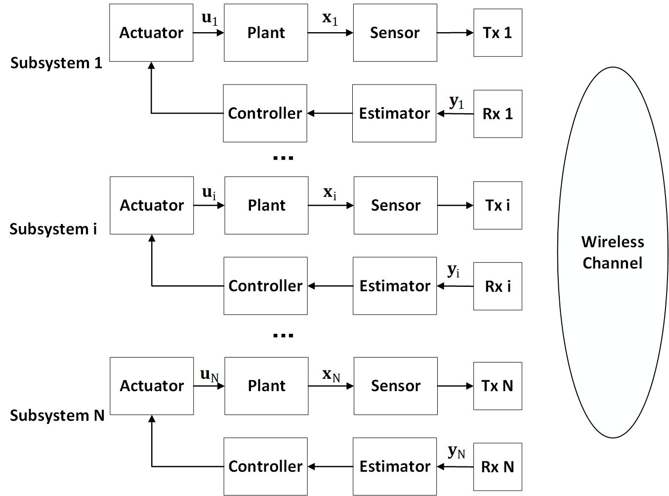
Figure 1: The multi-loop networked control systems model. Actuators and plants are wired to the controller while sensors and estimators communicate through a shared wireless network.

II-A System Setup

We consider the dynamic of the $i$-th subsystem at time slot $k$ is represented by the following discrete time LTI model:

$$\mathbf{x}_{i}[k+1]=\mathbf{A}_{i}\mathbf{x}_{i}[k]+\mathbf{B}_{i}\mathbf{u}_{i}[k]+\mathbf{e}_{i}[k]$$ (1)

with system state $\mathbf{x}_{i}$, control vector $\mathbf{u}_{i}$, system matrix $\mathbf{A}_{i}$ and input matrix $\mathbf{B}_{i}$ determined by the plant. And the system noise $\mathbf{e}_{i}$ is assumed to be an i.i.d. vector which has zero mean Gaussian distribution with diagonal covariance matrix $\mathbf{R}_{i}$. And each system has a initial state $\mathbf{x}_{i}[0]$ which is known at the controller side.

II-B Network Model

Figure 2 shows how our network model works. In time slot $k$, the scheduler allocates $M$ channel resources to specific subsystems according to the scheduling policy and unscheduled subsystems remain silent. According to assumption (iv), the channel state distribution of each subsystem is an i.i.d bernoulli distribution with expectation $p$. we denote the state observation received by the estimator as $\mathbf{y}_{i}[k]$. $\mathbf{y}_{i}[k]=\mathbf{x}_{i}[k]$ if and only if subsystem $i$ is scheduled to transmit in time slot $k$ and the transmittion is successful, otherwise $\mathbf{y}_{i}[k]=\text{NA}$.

Packets in networked control systems are time sensitive where stale control information may degrade performance of control loops. Thus, the freshness of information, i.e. the time difference bewteen generation and arrival, is one of the most important communication metric. Age of information(AoI) is often used to describe freshness of packets in systems. If at any time slot $k$, the freshest packet received by the controller of system $i$ is generated at time slot $G_{i}[k]$, the AoI in system $i$ at time slot $k$ is defined as:

$$\Delta_{i}[k]=k-G_{i}[k]$$ (2)

From the definition in (2), we can see that AoI is directly associated with the process of scheduling policy and channel state which will influence information update, and represents the freshness of system state information.

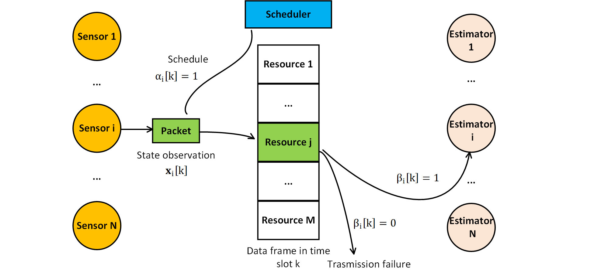
Figure 2: The wireless network model in time slot $k$.

II-C Controller and Estimator Model

According to assumption (iii), control vector $\mathbf{u}_{i}[k]$ at time slot $k$ is generated by the system state at the same time slot and then fed back to the plants to stabilize corresponding subsystems. In this paper, we suppose all subsystems have taken the deterministic control law as follows:

$$\mathbf{u}_{i}[k]=\mathbf{K}_{i}\hat{\mathbf{x}}_{i}[k]$$ (3)

where $\mathbf{K}_{i}$ is the stationary control gain determined by the control strategy and $\hat{\mathbf{x}}_{i}[k]$ is the estimation of subsystem $i$’s state at time slot $k$.

The principle of estimation is as follows: If the packet of subsystem $i$ in time slot $k$ has been received successfully, the estimator can directly use the state observation $\mathbf{y}_{i}[k]$ as the estimation, otherwise it will use the estimation of the last time slot $\hat{\mathbf{x}}_{i}[k-1]$ to iterate. $\alpha_{i}[k]$ and $\beta_{i}[k]$ are used to describe the scheduling result and channel state of subsystem $i$ on time slot $k$ respectively. Namely, $\alpha_{i}[k]=1$ means subsystem $i$ can transmit its state observation at time slot $k$ based on the scheduling result and $\beta_{i}[k]=1$ means subsystem $i$ can successfully transmit its data at time slot $k$. If $\alpha_{i}[k]=1$ and $\beta_{i}[k]=1$, we have $\mathbf{y}_{i}[k]=\alpha_{i}[k]\beta_{i}[k]\mathbf{x}_{i}[k]$. Thus, the dynamics of the estimator can be written as:

$$\hat{\mathbf{x}}_{i}[k] =\alpha_{i}(k)\beta_{i}(k)\mathbf{x}_{i}[k]+$$ (4)

$$(1-\alpha_{i}(k)\beta_{i}(k))(\mathbf{A}_{i}\hat{\mathbf{x}}_{i}[k-1]+\mathbf{B}_{i}\mathbf{K}_{i}\hat{\mathbf{x}}_{i}[k-1])$$

Then by combining (1), (3) and (4), the whole system dynamics is:

$$\left\{\begin{array}[]{lr}\mathbf{x}_{i}[k+1]=\mathbf{A}_{i}\mathbf{x}_{i}[k]+\mathbf{B}_{i}\mathbf{u}_{i}[k]+\mathbf{e}_{i}[k],&\\ \mathbf{u}_{i}[k]=\mathbf{K}_{i}\hat{\mathbf{x}}_{i}[k],&\\ \hat{\mathbf{x}}_{i}[k]=\alpha_{i}(k)\beta_{i}(k)\mathbf{x}_{i}[k]+&\\ (1-\alpha_{i}(k)\beta_{i}(k))(\mathbf{A}_{i}\hat{\mathbf{x}}_{i}[k-1]+\mathbf{B}_{i}\mathbf{K}_{i}\hat{\mathbf{x}}_{i}[k-1])&\end{array}\right.$$ (5)

III Control Performance Metrics

We first consider Linear Quadratic average-cost criterion [13] which can describe the control performance of each subsystem as:

$$J_{i} =\lim_{T\to+\infty}\frac{1}{T}\sum_{k=1}^{T}\mathbb{E}\{{\mathbf{x}_{i}}^{\mathbf{T}}[k]\mathbf{Q}_{i}\mathbf{x}_{i}[k]+{\mathbf{u}_{i}}^{\mathbf{T}}[k]\mathbf{P}_{i}{\mathbf{u}_{i}}[k]\}$$ (6)

where $\mathbf{Q}_{i}$ represents the state weights matrix of subsystem $i$ and $\mathbf{P}_{i}$ represents the control energy weights matrix of subsystem $i$.

And the sum cost is considered as the overall criterion to evaluate the performance of all subsystems

$$J =\sum_{i=1}^{N}J_{i}$$ (7)

$$=\lim_{T\to+\infty}\frac{1}{T}\sum_{i=1}^{N}\sum_{k=1}^{T}\mathbb{E}\{{\mathbf{x}_{i}}^{\mathbf{T}}[k]\mathbf{Q}_{i}\mathbf{x}_{i}[k]+{\mathbf{u}_{i}}^{\mathbf{T}}[k]\mathbf{P}_{i}{\mathbf{u}_{i}}[k]\}$$

Once the control strategy is determined, there will be a corresponding LQ cost. Non-ideal communication will affect the control effect and make systems deviate from the established design. We define this performance deviation, which we called as Linear Quadratic cost offset, as a control metric of the performance offset between ideal and non-ideal communication WNCSs. If we set $\mathbf{x}_{\text{opt},i}[k]$ and $\mathbf{u}_{\text{opt},i}[k]$ as the ideal system state and control vector when there are zero packet-drop and unlimited slot resources in time interval $[k-\Delta_{i}[k],k]$, the error between non-ideal state and ideal state is $\overline{\mathbf{x}}_{i}[k]=\mathbf{x}_{i}[k]-\mathbf{x}_{\text{opt},i}[k]$. Noted that when the system observation has been transmitted successfully in time slot $k-\Delta_{i}[k]$, we have $\overline{\mathbf{x}}_{i}[k-\Delta_{i}[k]]=0$. Therefore the Linear Quadratic cost offset is defined as:

$$J_{\text{offset}}= \lim_{T\to+\infty}\frac{1}{T}\sum_{i=1}^{N}\sum_{k=1}^{T}\mathbb{E}\{{\mathbf{x}_{i}}^{\mathbf{T}}[k]\mathbf{Q}_{i}\mathbf{x}_{i}[k]+{\mathbf{u}_{i}}^{\mathbf{T}}[k]\mathbf{P}_{i}{\mathbf{u}_{i}}[k]$$ (8)

$$-{\mathbf{x}_{\text{opt},i}}^{\mathbf{T}}[k]\mathbf{Q}_{i}\mathbf{x}_{\text{opt},i}[k]+{\mathbf{u}_{\text{opt},i}}^{\mathbf{T}}[k]\mathbf{P}_{i}{\mathbf{u}_{\text{opt},i}}[k]\}$$

This metric actually represents the average accumulated performance gap induced by non-ideal communication as time proceeded.

IV Analysis of Control Cost Offset and AoI

In this section, we will analyse the relationship between cost offset metric and Age of Information.

Lemma 1.

For the WNCSs described in (4) and (5), the state $\mathbf{x}_{i}[k]$ in subsystem $i$ at time slot $k$ with nonzero AoI $\Delta_{i}[k]$ has the following form:

$$\mathbf{x}_{i}[k] =(\mathbf{A}_{i}+\mathbf{B}_{i}\mathbf{K}_{i})^{\Delta_{i}[k]}\mathbf{x}_{i}[k-\Delta_{i}[k]]$$ (9)

$$+\sum_{j=0}^{\Delta_{i}[k]-1}{\mathbf{A}_{i}}^{j}\mathbf{e}_{i}[k-j-1]$$

Proof.

Nonzero $\Delta_{i}[k]$ means that estimator has successfully received the actual state $\mathbf{x}_{i}[k-\Delta_{i}[k]]$ at time slot $k-\Delta_{i}[k]$ and from that time slot on this subsystem did not get any state updated. Thus from (4), we can easily obtain the state estimation $\hat{\mathbf{x}}_{i}[k]$ as:

$$\hat{\mathbf{x}}_{i}[k]=(\mathbf{A}_{i}+\mathbf{B}_{i}\mathbf{K}_{i})^{\Delta_{i}[k]}\mathbf{x}_{i}[k-\Delta_{i}[k]]$$

Applying the system dynamics (5) and the estimation above, we can get the state $\mathbf{x}_{i}[k]$ iteratively.

$$\mathbf{x}_{i}[k-\Delta_{i}[k]+1] =(\mathbf{A}_{i}+\mathbf{B}_{i}\mathbf{K}_{i})\mathbf{x}_{i}[k-\Delta_{i}[k]]$$

$$+\mathbf{e}_{i}[k-\Delta_{i}[k]]$$

$$\mathbf{x}_{i}[k-\Delta_{i}[k]+2] =\mathbf{A}_{i}\mathbf{x}_{i}[k-\Delta_{i}[k]+1]$$

$$+\mathbf{B}_{i}\mathbf{K}_{i}(\mathbf{A}_{i} +\mathbf{B}_{i}\mathbf{K}_{i})\mathbf{x}_{i}[k-\Delta_{i}[k]]+\mathbf{e}_{i}[k-\Delta_{i}[k]+1]$$

$$=(\mathbf{A}_{i}+\mathbf{B}_{i}\mathbf{K}_{i})^{2}\mathbf{x}_{i}[k-\Delta_{i}[k]]$$

$$+\mathbf{A}_{i}\mathbf{e}_{i}[k-\Delta_{i}[k]]+\mathbf{e}_{i}[k-\Delta_{i}[k]+1]$$

$$......$$

$$\mathbf{x}_{i}[k-\Delta_{i}[k]+l] =(\mathbf{A}_{i}+\mathbf{B}_{i}\mathbf{K}_{i})^{l}\mathbf{x}_{i}[k-\Delta_{i}[k]]$$

$$+\sum_{j=0}^{l-1}{\mathbf{A}_{i}}^{j}\mathbf{e}_{i}[k-j-1]$$

$$......$$

$$\mathbf{x}_{i}[k] =(\mathbf{A}_{i}+\mathbf{B}_{i}\mathbf{K}_{i})^{\Delta_{i}[k]}\mathbf{x}_{i}[k-\Delta_{i}[k]]$$

$$+\sum_{j=0}^{\Delta_{i}[k]-1}{\mathbf{A}_{i}}^{j}\mathbf{e}_{i}[k-j-1]$$

∎

The offset between non-ideal state and ideal state can be derived from system dynamics and Lemma 1, leading to the following lemma.

Lemma 2.

For NCSs described in (5), the state offset in system $i$ at time slot $k$ can be written as:

$$\overline{\mathbf{x}}_{i}[k]=\sum_{j=0}^{\Delta_{i}[k]-1}({\mathbf{A}_{i}}^{j}-{(\mathbf{A}_{i}+\mathbf{B}_{i}\mathbf{K}_{i})}^{j})\mathbf{e}_{i}[k-j-1]$$ (10)

Proof.

Consider the ideal conditon where $\alpha$ and $\beta$ are always one and the non-ideal condition where systems have nonzero AOI, $\Delta_{i}[k]$, caused by scheduling and packet loss. The offset accumulates from time slot $k-\Delta_{i}[k]$ to time slot $k$. Using Lemma 1 and (5), the state offset is:

$$\overline{\mathbf{x}}_{i}[k] =\mathbf{x}_{i}[k]-\mathbf{x}_{\text{opt},i}[k]$$

$$=(\mathbf{A}_{i}+\mathbf{B}_{i}\mathbf{K}_{i})^{\Delta_{i}[k]}\mathbf{x}_{i}[k-\Delta_{i}[k]]$$

$$+\sum_{j=0}^{\Delta_{i}[k]-1}{\mathbf{A}_{i}}^{j}\mathbf{e}_{i}[k-j-1]$$

$$-(\mathbf{A}_{i}+\mathbf{B}_{i}\mathbf{K}_{i})^{\Delta_{i}[k]}\mathbf{x}_{i}[k-\Delta_{i}[k]]$$

$$-\sum_{j=0}^{\Delta_{i}[k]-1}{(\mathbf{A}_{i}+\mathbf{B}_{i}\mathbf{K}_{i})}^{j}\mathbf{e}_{i}[k-j-1]$$

$$=\sum_{j=0}^{\Delta_{i}[k]-1}({\mathbf{A}_{i}}^{j}-{(\mathbf{A}_{i}+\mathbf{B}_{i}\mathbf{K}_{i})}^{j})\mathbf{e}_{i}[k-j-1]$$

∎

It can be easily seen from Lemma 2 that, when $\Delta_{i}[k]=1$, the state offset is zero as well. In this situation, performance of this system doesn’t get degraded beacuse the state in time slot $k$ is generated from the state in time slot $k-1$, which is successfully updated. Transmission status in time slot $k$ will affect system states in time slot $k+1$. So scheduling in current time slot will influence the performance of our WNCSs in the next time slot.

Remark 1.

As ${e}_{i}[k]$ is i.i.d. zero-mean gaussian noise, it is obvious that the state error $\overline{\mathbf{x}}_{i}[k]$ which is the linear combination of Gaussian noise, has a Gaussian distribution and zero expectation, $\mathbb{E}[\overline{\mathbf{x}}_{i}[k]]=0$.

By using previous lemmas and the definition of LQ cost offset metric, we can get the following result about our metric and AoI.

Lemma 3.

For WNCSs described in (5) and cost offset metric described in (8), the time average Linear Quadratic cost offset in subsystem $i$ at time slot $k$ can be written as:

$$J_{\text{offset}} =\lim_{T\to+\infty}\frac{1}{T}\sum_{i=1}^{N}\sum_{k=1}^{T}\sum_{j=0}^{\Delta_{i}[k]-1}\mathbf{Tr}\{\left[\mathbf{Q}_{i}+{\mathbf{K}_{i}}^{\mathbf{T}}\mathbf{P}_{i}\mathbf{K}_{i}\right]$$ (11)

$${({\mathbf{A}_{i}}^{j}-{(\mathbf{A}_{i}+\mathbf{B}_{i}\mathbf{K}_{i})}^{j})}\mathbf{R}_{i}{({\mathbf{A}_{i}}^{j}-{(\mathbf{A}_{i}+\mathbf{B}_{i}\mathbf{K}_{i})}^{j})}^{T}\}$$

Proof.

Using lemma 2 and elementary matrix caculation, we can derive the following form of the LQ offset.

$$J_{\text{offset}} =\lim_{T\to+\infty}\frac{1}{T}\sum_{i=1}^{N}\sum_{k=1}^{T}\mathbb{E}\{{\mathbf{x}_{i}}^{\mathbf{T}}[k](\mathbf{Q}_{i}+{\mathbf{K}_{i}}^{\mathbf{T}}\mathbf{P}_{i}\mathbf{K}_{i})\mathbf{x}_{i}[k]-$$

$${\mathbf{x}_{\text{opt},i}}^{\mathbf{T}}[k](\mathbf{Q}_{i}+{\mathbf{K}_{i}}^{\mathbf{T}}\mathbf{P}_{i}\mathbf{K}_{i})\mathbf{x}_{\text{opt},i}[k]\}$$

$$=\lim_{T\to+\infty}\frac{1}{T}\sum_{i=1}^{N}\sum_{k=1}^{T}\mathbb{E}\{{\mathbf{x}_{i}}^{\mathbf{T}}[k](\mathbf{Q}_{i}+{\mathbf{K}_{i}}^{\mathbf{T}}\mathbf{P}_{i}\mathbf{K}_{i})\mathbf{x}_{i}[k]-$$

$${(\mathbf{x}_{i}+\overline{\mathbf{x}}_{i}[k])}^{\mathbf{T}}(\mathbf{Q}_{i}+{\mathbf{K}_{i}}^{\mathbf{T}}\mathbf{P}_{i}\mathbf{K}_{i})(\mathbf{x}_{i}+\overline{\mathbf{x}}_{i}[k])\}$$

$$=\lim_{T\to+\infty}\frac{1}{T}\sum_{i=1}^{N}\sum_{k=1}^{T}\mathbb{E}\{{\overline{\mathbf{x}}_{i}}^{\mathbf{T}}[k](\mathbf{Q}_{i}+{\mathbf{K}_{i}}^{\mathbf{T}}\mathbf{P}_{i}\mathbf{K}_{i})\overline{\mathbf{x}}_{i}[k]\}$$

$$=\lim_{T\to+\infty}\frac{1}{T}\sum_{i=1}^{N}\sum_{k=1}^{T}\mathbb{E}\{\mathbf{Tr}\{[{\sum_{j=0}^{\Delta_{i}[k]-1}(\mathbf{Q}_{i}+{\mathbf{K}_{i}}^{\mathbf{T}}\mathbf{P}_{i}\mathbf{K}_{i})}$$

$$({\mathbf{A}_{i}}^{j}-{(\mathbf{A}_{i}+\mathbf{B}_{i}\mathbf{K}_{i})}^{j}){\mathbf{e}_{i}[k-j-1]{\mathbf{e}_{i}[k-j-1]}^{\mathbf{T}}}$$

$${{({\mathbf{A}_{i}}^{j}-{(\mathbf{A}_{i}+\mathbf{B}_{i}\mathbf{K}_{i})}^{j})}^{\mathbf{T}}}\}\}$$

$$=\lim_{T\to+\infty}\frac{1}{T}\sum_{i=1}^{N}\sum_{k=1}^{T}\sum_{j=0}^{\Delta_{i}[k]-1}\mathbf{Tr}\{\left[\mathbf{Q}_{i}+{\mathbf{K}_{i}}^{\mathbf{T}}\mathbf{P}_{i}\mathbf{K}_{i}\right]$$

$${({\mathbf{A}_{i}}^{j}-{(\mathbf{A}_{i}+\mathbf{B}_{i}\mathbf{K}_{i})}^{j})}\mathbf{R}_{i}{({\mathbf{A}_{i}}^{j}-{(\mathbf{A}_{i}+\mathbf{B}_{i}\mathbf{K}_{i})}^{j})}^{T}\}$$

where $\mathbf{R}_{i}$ is the covariance matrix of Gaussian noise in subsystem $i$. ∎

As we can see from lemma 3, the linear quadratic cost offset is a kind of non-linear function of AoI process, which means that the process of Age of Information and the system parameters determine the performance offset of our WNCSs.

V An Age-based Scheduling Method

Non-ideal communication network means constraints on communication resources so that transmission needs for all subsystems cannot be satified simultaneously. Employing effective scheduling policy can optimize resources allocation and therefore improve WNCSs performance. Suppose the information set availabe at the scheduler is $\mathbb{I}_{S}[k]=\{{\{{\mathbf{A}}_{i}\}}_{i=1}^{N},{\{{\mathbf{B}}_{i}\}}_{i=1}^{N},{\{{\mathbf{K}}_{i}\}}_{i=1}^{N},{\{{\mathbf{R}}_{i}\}}_{i=1}^{N},{\{\Delta_{i}[k]\}}_{i=1}^{N}\}$. Based on the theory above, we propose an AoI-based scheduling problem which aims to minimize our proposed control cost offset:

$$\min_{{\alpha[k]}} J_{\text{offset}}$$ (13)

s.t. $$\sum_{i=1}^{N}{\alpha_{i}}[k]\leq M$$

It’s obvious that this is an infinite horizon integer programming. It’s hard to solve this infinite horizon problem in polynomial time, so we come up with a greedy solution to solve it. As scheduling in current time slot will influence the performance of our WNCSs in the next time slot. we try to minimize total control cost offset contribution of all sub-systems in every time slot $k$ by picking M sub-systems which have maximum expected control cost offsets $J_{\text{offset},i}[k]$:

$$J_{\text{offset},i}[k] =\sum_{j=0}^{\Delta_{i}[k]}\mathbb{E}\{\mathbf{Tr}\{\left[\mathbf{Q}_{i}+{\mathbf{K}_{i}}^{\mathbf{T}}\mathbf{P}_{i}\mathbf{K}_{i}\right]$$ (14)

$${({\mathbf{A}_{i}}^{j}-{(\mathbf{A}_{i}+\mathbf{B}_{i}\mathbf{K}_{i})}^{j})}\mathbf{R}_{i}{({\mathbf{A}_{i}}^{j}-{(\mathbf{A}_{i}+\mathbf{B}_{i}\mathbf{K}_{i})}^{j})}^{T}\}\}$$

And the greedy optimization problem is:

$$\max_{{\alpha[k]}} \sum_{i=1}^{N}\alpha_{i}[k]J_{\text{offset},i}[k]$$ (15)

s.t. $$\sum_{i=1}^{N}{\alpha_{i}}[k]\leq M$$

The scheduling policy is given in algorithm 1.

Algorithm 1 Framework of our scheduling policy for WNCSs.

0:    The parameters of all N subsystems, ${\{{\mathbf{A}}_{i}\}}_{i=1}^{N}$, ${\{{\mathbf{B}}_{i}\}}_{i=1}^{N}$, ${\{{\mathbf{K}}_{i}\}}_{i=1}^{N}$; The set of Age of information of all N subsystems at time slot $k$, ${\{\Delta_{i}[k]\}}_{i=1}^{N}$;The covariance matrices of noise of all N subsystems, ${\{{\mathbf{R}}_{i}\}}_{i=1}^{N}$;

0:    The set of scheduling states, $\bm{\alpha}[k]$;

1:  Initializing scheduling states with $\alpha_{i}[k]=0$;

2:  Calculating expected control cost offsets $J_{\text{offset},i}[k]$ with the help of $\mathbf{A}_{i}$, $\mathbf{B}_{i}$, $\mathbf{K}_{i}$, $\mathbf{R}_{i}$ and $\Delta_{i}[k]$;

3:  Extracting M sub-systems with the largest offsets $J_{\text{offset},i}[k]$ and put their scheduling states with value 1;

4:  return  $\bm{\alpha}[k]$;

In the next section, we show that our proposed scheduling policy has performance advantages in LQ cost offset metric compared to other existed scheduling policies.

VI Numerical Results

To illustrate our proposed scheduling policy, we now continue with giving simulations.

VI-A Simulation Setup

Empiric cost is used to approximately represent our proposed cost offset criterion and average-cost criterion for ease of calculation, and can be calculated by:

$$J_{\text{offset}}\approx\frac{1}{T}\sum_{i=1}^{N}\sum_{k=1}^{T}\sum_{j=0}^{\Delta_{i}[k]-1}\mathbf{Tr}\{\left[\mathbf{Q}_{i}+{\mathbf{K}_{i}}^{\mathbf{T}}\mathbf{P}_{i}\mathbf{K}_{i}\right]$$ (16)

$${({\mathbf{A}_{i}}^{j}-{(\mathbf{A}_{i}+\mathbf{B}_{i}\mathbf{K}_{i})}^{j})}\mathbf{R}_{i}{({\mathbf{A}_{i}}^{j}-{(\mathbf{A}_{i}+\mathbf{B}_{i}\mathbf{K}_{i})}^{j})}^{T}\}$$

$$J\approx\frac{1}{T}\sum_{i=1}^{N}\sum_{k=1}^{T}\mathbb{E}\{{\mathbf{x}_{i}}^{\mathbf{T}}[k]\mathbf{Q}_{i}\mathbf{x}_{i}[k]+{\mathbf{u}_{i}}^{\mathbf{T}}[k]\mathbf{P}_{i}{\mathbf{u}_{i}}[k]\}$$

where $T=5000$ is the simulation time length in our work.

We perform simulations where $N=8$ subsystems sharing the wireless network and scheduler makes full use of historical information $\mathbb{I}_{S}[k]$ to decide which sub-systems should transmit their states. The parameters and control laws of all eight subsystems we considered are shown in Table I and Table II. Furthermore, the initial state is given with the deterministic initial value $\mathbf{x}_{i}[0]={[1,1]}^{T}$.

To evaluate our policy, we introduce four different scheduling policies to compare.

• AOI-minimal policy In every time slot, the scheduler chooses $M$ subsystems with the maximal AOI to transmit. As the conclusion in [8], this greedy scheduling is age-optimal.

• Estimation error minimal policy In every time slot, the scheduler chooses $M$ subsystems with the maximal quadratic state estimation error[1] to transmit.

• Round-Robin policy In every time slot, the scheduler allocates the communication resources sequentially.

• Random policy In every time slot, the scheduler randomly chooses $M$ subsystems to transmit.

VI-B Time sensitive systems

Firstly, we consider a time sensitive system where most subsystems have a system state matrix with eigenvalues of which real part is larger than one, which means that they will suffer perfermance loss if there is no fresh state information updated. In the mean time, different systems will bring different contributions to the control cost in the form of different $\mathbf{Q}_{i}$. The parameters and control laws of such system are showed in Table I.

TABLE I: System Parameters and control laws of time sensitive systems

$i$	$\mathbf{A}_{i}$	$\mathbf{B}_{i}$	$\mathbf{Q}_{i}$	$\mathbf{P}_{i}$	$\mathbf{R}_{i}$	$\mathbf{K}_{i}$
1	$1.1*\mathbf{S}$	$\mathbf{I}$	$100*\mathbf{I}$	$\mathbf{I}$	$0.25*\mathbf{I}$	$-0.2*\mathbf{I}$
2	$1.1*\mathbf{S}$	$\mathbf{I}$	$100*\mathbf{I}$	$\mathbf{I}$	$0.25*\mathbf{I}$	$-0.3*\mathbf{I}$
3	$1.2*\mathbf{S}$	$\mathbf{I}$	$10*\mathbf{I}$	$\mathbf{I}$	$0.25*\mathbf{I}$	$-0.4*\mathbf{I}$
4	$1.2*\mathbf{S}$	$\mathbf{I}$	$8*\mathbf{I}$	$\mathbf{I}$	$0.25*\mathbf{I}$	$-0.6*\mathbf{I}$
5	$1.3*\mathbf{S}$	$\mathbf{I}$	$6*\mathbf{I}$	$\mathbf{I}$	$0.25*\mathbf{I}$	$-0.8*\mathbf{I}$
6	$1.3*\mathbf{S}$	$\mathbf{I}$	$4*\mathbf{I}$	$\mathbf{I}$	$0.25*\mathbf{I}$	$-1*\mathbf{I}$
7	$1.4*\mathbf{S}$	$\mathbf{I}$	$2*\mathbf{I}$	$\mathbf{I}$	$0.25*\mathbf{I}$	$-1.2*\mathbf{I}$
8	$1.4*\mathbf{S}$	$\mathbf{I}$	$\mathbf{I}$	$\mathbf{I}$	$0.25*\mathbf{I}$	$-1,2*\mathbf{I}$
where $\mathbf{I}=\begin{aligned} \left[\begin{array}[]{cc}1&0\\ 0&1\end{array}\right]\end{aligned}$ and $\mathbf{S}=\begin{aligned} \left[\begin{array}[]{cc}1&0.2\\ -0.2&1\end{array}\right]\end{aligned}$

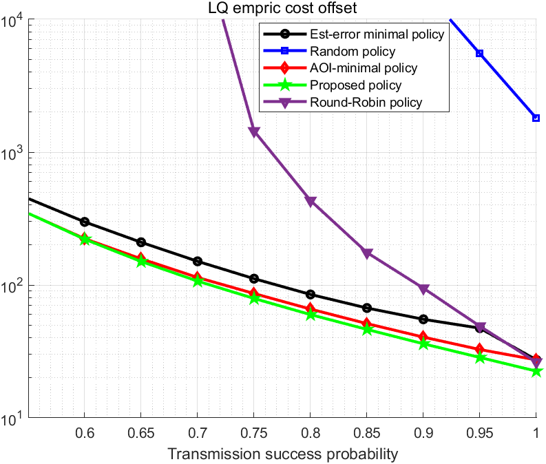
Figure 3: Cost offset comparison of the five types of scheduling policies with different channel states $p$ and $M=3$ wireless resources in time sensitive systems.

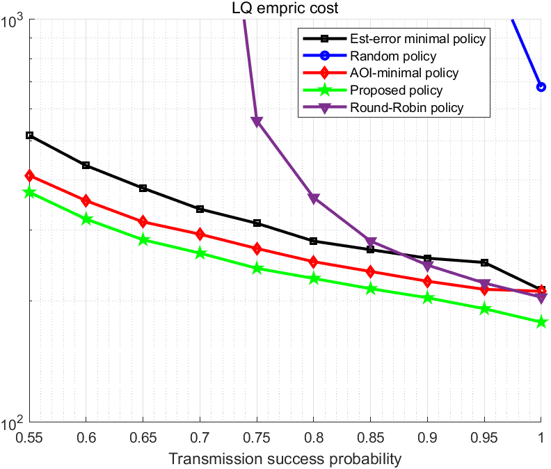
Figure 4: LQ cost comparison of the five types of scheduling policies with different channel states $p$ and $M=3$ wireless resources in time sensitive systems.

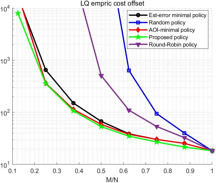
Figure 5: Cost offset comparison of the five types of scheduling policies with different wireless resources $M$ per time slot and transmission success rate $p=0.7$.

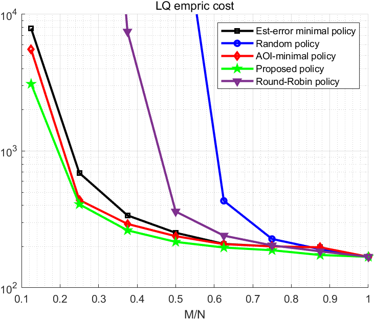
Figure 6: LQ cost comparison of the five types of scheduling policies with different wireless resources $M$ and transmission success rate $p=0.7$.

Figure 3 and Figure 5 compare linear quadratic empiric cost offset for AoI-minimal policy, Estimation error minimal policy, Round-Robin Policy, Random policy and our proposed policy which minimize real-time control offset of the whole systems in time sensitive scenarios. Different transmission success probabilities $p$ and resource ratios $\frac{M}{N}$ are considered, and it can be observed that random policy has the worst control performance. With the increase of trasmission success probability and resource ratios, the cost offsets gradually reduce. When transmission resources are abundant, all policies perform well beacause almost every system can be served in every time slot. We obtain some gain compared to the existed policies in such systems no matter what transmission conditions are.

Figure 4 and Figure 6 show comparison of linear quadratic empiric cost for the five types of policys. Same as the cost offset, our policy has an advantage in performance. In the meantime, it is worth mentioning that there is a similar characterization of performance, which means we could optimize our proposed cost offset of such systems to indirectly optimize the LQ cost to some extent. It will be helpful for system co-design because sometimes it is hard to solve complex control cost optimization.

VI-C Large characteristic time systems

On the other hand, we take stable systems with large characteristic time into consideration as well, which is shown in Table II. These stable systems are designed to have large characteristic time and therefore have better performance in the accuracy of control and noise immunity. We suppose that added feedback loops in some systems reduce the convergence speed and improves the noise immunity. For example, real part of eigenvalue of $\mathbf{A}_{1}$ is smaller than that of $\mathbf{A}_{1}+\mathbf{B}_{1}\mathbf{K}_{1}$.

TABLE II: System Parameters and control laws of stable systems with large characteristic time

$i$	$\mathbf{A}_{i}$	$\mathbf{B}_{i}$	$\mathbf{Q}_{i}$	$\mathbf{P}_{i}$	$\mathbf{R}_{i}$	$\mathbf{K}_{i}$
1	$0.1*\mathbf{S}$	$\mathbf{I}$	$\mathbf{I}$	$\mathbf{I}$	$0.25*\mathbf{I}$	$0.8*\mathbf{I}$
2	$0.1*\mathbf{S}$	$\mathbf{I}$	$\mathbf{I}$	$\mathbf{I}$	$0.25*\mathbf{I}$	$0.75*\mathbf{I}$
3	$0.2*\mathbf{S}$	$\mathbf{I}$	$\mathbf{I}$	$\mathbf{I}$	$0.25*\mathbf{I}$	$0.5*\mathbf{I}$
4	$0.2*\mathbf{S}$	$\mathbf{I}$	$\mathbf{I}$	$\mathbf{I}$	$0.25*\mathbf{I}$	$0.455*\mathbf{I}$
5	$0.3*\mathbf{S}$	$\mathbf{I}$	$\mathbf{I}$	$\mathbf{I}$	$0.25*\mathbf{I}$	$-0.05*\mathbf{I}$
6	$0.3*\mathbf{S}$	$\mathbf{I}$	$\mathbf{I}$	$\mathbf{I}$	$0.25*\mathbf{I}$	$-0.1*\mathbf{I}$
7	$0.4*\mathbf{S}$	$\mathbf{I}$	$\mathbf{I}$	$\mathbf{I}$	$0.25*\mathbf{I}$	$-0.35*\mathbf{I}$
8	$0.4*\mathbf{S}$	$\mathbf{I}$	$\mathbf{I}$	$\mathbf{I}$	$0.25*\mathbf{I}$	$-0.38*\mathbf{I}$
where $\mathbf{I}=\begin{aligned} \left[\begin{array}[]{cc}1&0\\ 0&1\end{array}\right]\end{aligned}$ and $\mathbf{S}=\begin{aligned} \left[\begin{array}[]{cc}1&0.2\\ -0.2&1\end{array}\right]\end{aligned}$

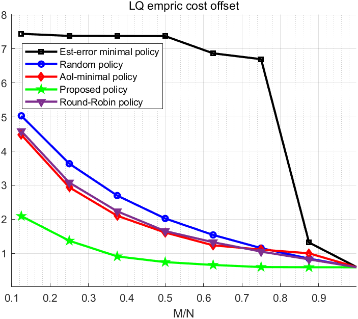
Figure 7: LQ cost comparison of the five types of scheduling policies with different resource allocation rates and 0.7 transmission success probabilities.

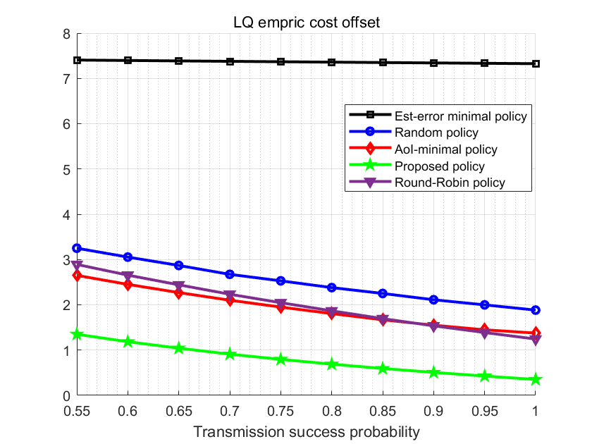
Figure 8: LQ cost comparison of the five types of scheduling policies with different transmission success rates and $M=3$ wireless resources.

From Figure 7 and Figure 8, we can see that compared to the time sensitive systems situation, our proposed policy obtains much more gains in cost offset criterion. As cost offset criterion indicates the offset between actual situation and the ideal design, our proposed policy has better performance in mitigating non-ideal communication loss. Furthermore, Estimation error minimal policy has a deteriorating performance due to limitations of simply optimizing estimation error.

VII Conclusion and Furture Work

This paper has studied multi-loop wireless networked control systems which share a common wireless channel, presented a new metric criterion to descirbe the performance offset between situations with ideal communication and non-ideal communication, and has proposed a scheduling policy which at every time slot chooses subsystems with maximum expected offset cost to transmit. Simulation results show that compared to existed policies, our proposed policy may help to improve control performance in many different WNCSs cases. Other future research directions include partial state transmission scheduling, distributed control transmission scheme design and control law design based on the process of AoI.

References

- [1] Onur Ayan, Mikhail Vilgelm, Markus Klügel, Sandra Hirche, and Wolfgang Kellerer. Age-of-information vs. value-of-information scheduling for cellular networked control systems. In Proceedings of the 10th ACM/IEEE International Conference on Cyber-Physical Systems, pages 109–117. ACM, 2019.
- [2] Anton Cervin and Toivo Henningsson. Scheduling of event-triggered controllers on a shared network. In 2008 47th IEEE Conference on Decision and Control, pages 3601–3606. IEEE, 2008.
- [3] Jaya Prakash Champati, Mohammad H Mamduhi, Karl H Johansson, and James Gross. Performance characterization using aoi in a single-loop networked control system. arXiv preprint arXiv:1901.06694, 2019.
- [4] Emanuele Garone, Bruno Sinopoli, Andrea Goldsmith, and Alessandro Casavola. Lqg control for mimo systems over multiple erasure channels with perfect acknowledgment. IEEE Transactions on Automatic Control, 57(2):450–456, 2011.
- [5] Arash Hassibi, Stephen P Boyd, and Jonathan P How. Control of asynchronous dynamical systems with rate constraints on events. In Proceedings of the 38th IEEE Conference on Decision and Control (Cat. No. 99CH36304), volume 2, pages 1345–1351. IEEE, 1999.
- [6] Erik Henriksson, Daniel E Quevedo, Edwin GW Peters, Henrik Sandberg, and Karl Henrik Johansson. Multiple-loop self-triggered model predictive control for network scheduling and control. IEEE Transactions on Control Systems Technology, 23(6):2167–2181, 2015.
- [7] Kang Huang, Wanchun Liu, Yonghui Li, and Branka Vucetic. To retransmit or not: Real-time remote estimation in wireless networked control. arXiv preprint arXiv:1902.07820, 2019.
- [8] Igor Kadota, Abhishek Sinha, Elif Uysal-Biyikoglu, Rahul Singh, and Eytan Modiano. Scheduling policies for minimizing age of information in broadcast wireless networks. IEEE/ACM Transactions on Networking (TON), 26(6):2637–2650, 2018.
- [9] Gruteser M Kaul S, Yates R. Real-time status: How often should one update? In IEEE INFOCOM. IEEE, 2012, pages 2731–2735. IEEE, 2012.
- [10] Dong-Sung Kim, Young Sam Lee, Wook Hyun Kwon, and Hong Seong Park. Maximum allowable delay bounds of networked control systems. Control Engineering Practice, 11(11):1301–1313, 2003.
- [11] Husheng Li, Ju Bin Song, and Qi Zeng. Adaptive modulation in networked control systems with application in smart grids. IEEE Communications Letters, 17(7):1305–1308, 2013.
- [12] Adam Molin and Sandra Hirche. On lqg joint optimal scheduling and control under communication constraints. In Proceedings of the 48h IEEE Conference on Decision and Control (CDC) held jointly with 2009 28th Chinese Control Conference, pages 5832–5838. IEEE, 2009.
- [13] Adam Molin and Sandra Hirche. Price-based adaptive scheduling in multi-loop control systems with resource constraints. IEEE Transactions on Automatic Control, 59(12):3282–3295, 2014.
- [14] CL Robinson and PR Kumar. Sending the most recent observation is not optimal in networked control: Linear temporal coding and towards the design of a control specific transport protocol. In 2007 46th IEEE Conference on Decision and Control, pages 334–339. IEEE, 2007.
- [15] Alberto Tarable, Alessandro Nordio, Fabrizio Dabbene, and Roberto Tempo. Anytime reliable ldpc convolutional codes for networked control over wireless channel. In 2013 IEEE International Symposium on Information Theory, pages 2064–2068. IEEE, 2013.
- [16] Gregory C Walsh, Hong Ye, and Linda G Bushnell. Stability analysis of networked control systems. IEEE transactions on control systems technology, 10(3):438–446, 2002.
- [17] Yang Xu, Karl-Erik Årzén, Enrico Bini, and Anton Cervin. Lqg-based control and scheduling co-design. IFAC-PapersOnLine, 50(1):5895–5900, 2017.