Towards Spatial Bisimilarity for Closure Models:
Logical and Coalgebraic Characterisations

Abstract

The topological interpretation of modal logics provides descriptive languages and proof systems for reasoning about points of topological spaces. Recent work has been devoted to model checking of spatial logics on discrete spatial structures, such as finite graphs and digital images, with applications in various case studies including medical image analysis. These recent developments required a generalization step, from topological spaces to closure spaces. In this work we initiate the study of bisimilarity and minimization algorithms that are consistent with the closure spaces semantics. For this purpose we employ coalgebraic models. We present a coalgebraic definition of bisimilarity for quasi-discrete models, which is adequate with respect to a spatial logic with reachability operators, complemented by a free and open-source minimization tool for finite models. We also discuss the non-quasi-discrete case, by providing a generalization of the well-known set-theoretical notion of topo-bisimilarity, and a categorical definition, in the same spirit as the coalgebraic rendition of neighbourhood frames, but employing the covariant power set functor, instead of the contravariant one. We prove its adequacy with respect to infinitary modal logic.

patial Logics, Bisimilarity, Coalgebra, Closure Spaces.

1 Introduction

Traditional modal logic enjoys a topological interpretation, according to which the modal formula $\diamond\mkern 1.0mu\Phi$ is true at a point $x$ of a topological space, whenever $x$ belongs to the topological closure of the set of points at which $\Phi$ is true. This fundamental observation has led to a variety of extensions of the basic framework, with different proof systems and computational properties, cf. [3].

Model checking has been studied for the case of spatial logics only recently. In order to retain the topological flavour, but aiming at analysis of more general structures, also encompassing graphs, the Spatial Logic for Closure Spaces ($\mathtt{SLCS}$) has been proposed by Ciancia et al. in [13] together with an algorithm for model checking of finite models. The logic $\mathtt{SLCS}$ is interpreted on closure spaces (a generalization of topological spaces where the closure operator is not necessarily idempotent). We refer the reader to [14] for a full account of the logic and its main features and properties – including its extension with a collective fragment. The logic and its model checkers topochecker [12] and VoxLogicA [8] have been applied to several case studies [14, 12, 11] including a declarative approach to medical image analysis [6, 8, 7, 4]. An encoding of the discrete Region Connection Calculus RCC8D of [24] into the collective variant of $\mathtt{SLCS}$ has been proposed in [15]. The logic has also inspired other approaches to spatial reasoning in the context of signal temporal logic and system monitoring [5, 23] and in the verification of cyber-physical systems [26].

In this work, we initiate the study of bisimilarity and minimization algorithms for spatial structures, employing equivalence relations on points of a closure space that are adequate with respect to spatial logical equivalence. That is, we require that two points are bisimilar if and only if they satisfy the same formulas of a (chosen) spatial logical language. For the topological case, one such equivalence has been provided by Aiello and Van Benthem [9], under the name of topo-bisimilarity. This relation is adequate with respect to logical equivalence of basic infinitary modal logic, i.e. a boolean logic with one modal operator, and infinitary conjunction/disjunction. In contrast, besides basic modalities, the logic $\mathtt{SLCS}$ features operators that make use of reachability via paths of bounded and unbounded length (for instance, the surrounded and touch operators of [14]). Although the study of such operators has not been developed in full detail in the classical spatial logics literature, they have proved useful in case studies. For instance, the ability to identify two areas, characterised by given logical formulas, that additionally are in contact with each other, while retaining the point-based approach of topo-logics, has been the key to derive a segmentation algorithm that labels brain tumours in three-dimensional medical images, with accuracy in par with manual segmentation, and best-in-class machine learning methods [8].

In the present paper, we focus on two different, related problems. First of all, we identify a spatial definition of bisimilarity for quasi-discrete models (those that correspond to graphs), and a minimization algorithm for finite models, in the setting of logics with reachability. This is directly aimed at supporting the future developments of the spatial model checking methodology that is currently in use, e.g. in [8]. In Section 3 we present a set-theoretical definition, and provide some examples. In Section 4, we provide a coalgebraic rendition of such an equivalence. In Section 5, we prove adequacy with respect to logical equivalence of a logic with two reachability operators (corresponding to the two directions of “reaching” and “being reached”). In Section 6 we introduce an open source tool that is able to minimize finite models via coalgebraic partition refinement.

The second research question that we address here, is whether the theory of topo-bisimilarity of [9], characterising infinitary modal logic (without reachability operators), can be generalised to closure models (not limited to the quasi-discrete ones). In Section 7, we first provide a consistent generalization, obtained by appropriately replacing the notion of an open neighbourhood with one that is equivalent in the restricted setting of topological spaces, but not in the more general one. The defined equivalence relation is adequate for infinitary modal logic when interpreted on closure spaces. Then, we provide a coalgebraic definition. We prove that logical equivalence of infinitary modal logic can be characterised as behavioural equivalence for coalgebras of the closure functor $\mathcal{P}(\mathcal{P}(-))$. The notion we propose is similar in spirit to neighbourhood frames (see [19]), although we use the covariant power set, therefore staying closer to the more classical literature on coalgebras in Computer Science.

Although the results we present are sound and stable, we consider them as a preliminary foundation. Future work will be devoted to the characterisation of logical equivalence for variants of the considered logics (for instance, those that cannot express one-step modalities, logics with distances, etc.). We provide some discussion on these matters in Section 8.

2 Preliminaries

Given set $X$ and relation $R\subseteq X\times X$, we let $R^{\,t}$ denote the transitive closure of $R$ and let $R^{-1}$ denote the inverse of $R$, i.e. $R^{-1}=\{\,(x_{1},x_{2})\mid(x_{2},x_{1})\in R\,\}$. For $x\in X$, we let $[x]_{R}$ denote the equivalence class of $x$ (we will omit the subscript whenever this does not cause confusion). We let $\mathcal{P}$ denote the covariant powerset functor; for $f:X\to Y$ and $A\subseteq X$, its action on arrows $\mathcal{P}f\,A$, often abbreviated to $f\,A$, is defined as $\{\,fa\mid a\in A\,\}$. Similarly, $\mathcal{P}_{\omega}X$ denotes the covariant finite powerset functor. For $f:X\to Y$ a function, we denote by $f^{-1}:\mathcal{P}Y\to\mathcal{P}X$ its “relational” inverse, that is the function mapping $B\subseteq Y$ to $\{x\in X\mid fx\in B\}$. We will often use currying for function type definitions and applications, when this does not create confusion.

Definition 1

A closure space is a pair $(X,{\cal C})$ where $X$ is a non-empty set (of points) and ${\cal C}:\mathcal{P}X\to\mathcal{P}X$ is a function satisfying the following axioms.

1. ${\cal C}\mkern 1.0mu\emptyset=\emptyset$

2. $A\subseteq{\cal C}\mkern 1.0muA$ for all $A\subseteq X$

3. ${\cal C}\mkern 1.0mu(A_{1}\cup A_{2})={\cal C}\mkern 1.0muA_{1}\cup{\cal C}\mkern 1.0muA_{2}$ for all $A_{1},A_{2}\subseteq X$

The definition of a closure space goes back to Eduard Čech. By the Kuratowski definition, topological spaces coincide with the sub-class of closure spaces for which also the idempotence axiom ${\cal C}\mkern 1.0mu({\cal C}\mkern 1.0muA)={\cal C}\mkern 1.0muA$ holds. The interior operator is the dual of closure: ${\cal I}\,A=\overline{{\cal C}\mkern 1.0mu(\overline{A})}$. Given a relation $R\subseteq X\times X$, the function ${\cal C}_{R}:\mathcal{P}X\to\mathcal{P}X$ with ${\cal C}_{R}\mkern 1.0mu(A)=A\cup\{\,x\mid\exists\mkern 1.0mua\in A\colon a\,R\,x\,\}$ satisfies the axioms of Definition 1, thus making $(X,{\cal C}_{R})$ a closure space. We say that $(X,{\cal C}_{R})$ is based on $R$. It can be shown that the sub-class of closure spaces that can be generated by a relation as above coincides with the class of quasi-discrete closure spaces, i.e. closure spaces where every $x\in X$ has a minimal neighbourhood or, equivalently, for each $A\subseteq X,\,{\cal C}\mkern 1.0muA=\bigcup_{a\in A}{\cal C}\mkern 1.0mu\{a\}$. Thus discrete structures, like graphs or Kripke structures can be seen as quasi-discrete closure spaces. With reference to a quasi-discrete closure space $(X,{\cal C}_{R})$ based on a relation $R$, we define the abbreviations $\stackrel{{\scriptstyle\rightarrow}}{{{\cal C}}},\stackrel{{\scriptstyle\leftarrow}}{{{\cal C}}}:X\to\mathcal{P}X$ by $\stackrel{{\scriptstyle\rightarrow}}{{{\cal C}}}\!\!x={\cal C}_{R}\mkern 1.0mu(\{x\})$ and $\stackrel{{\scriptstyle\leftarrow}}{{{\cal C}}}\!\!x={\cal C}_{{R^{-1}}}\mkern 1.0mu(\{x\})$.

Definition 2

A continuous function from closure space $(X_{1},{\cal C}_{1})$ to closure space $(X_{2},{\cal C}_{2})$ is a function $f:X_{1}\to X_{2}$ such that, for all sets $A\subseteq X_{1}$, it holds that $f({\cal C}_{1}\mkern 1.0muA)\subseteq{\cal C}_{2}\mkern 1.0mu(f\,A)$.

We fix a set $AP$ of atomic predicates. A closure model ${\cal M}=((X,{\cal C}),{\cal V})$ is a pair with $(X,{\cal C})$ a closure space, and ${\cal V}:AP\to\mathcal{P}X$ the (atomic predicate) valuation (function). We define ${\cal V}^{\mbox{-}\mkern-2.0mu\mbox{\scriptsize 1}}:\mathcal{P}X\to\mathcal{P}AP$ with ${\cal V}^{\mbox{-}\mkern-2.0mu\mbox{\scriptsize 1}}\mkern-1.5muA=\{\,p\in AP\mid\exists\mkern 1.0mua\in A\colon a\in{\cal V}\,p\,\}$ and we let ${\cal V}^{\mbox{-}\mkern-2.0mu\mbox{\scriptsize 1}}\mkern-1.5mu{x}$ abbreviate ${\cal V}^{\mbox{-}\mkern-2.0mu\mbox{\scriptsize 1}}\mkern-1.5mu{\{x\}}$. We say that a closure model ${\cal M}=((X,{\cal C}),{\cal V})$ is quasi-discrete if $(X,{\cal C})$ is quasi-discrete. A quasi-discrete closure model $((X,{\cal C}_{R}),{\cal V})$ is finitely closed if $\stackrel{{\scriptstyle\rightarrow}}{{{\cal C}}}\!\!{x}$ is finite for all $x\in X$. Similarly, we say that ${\cal M}$ is finitely backward closed if $\stackrel{{\scriptstyle\leftarrow}}{{{\cal C}}}\!\!{x}$ is finite for all $x\in X$.

In the following definition, $(\mathbb{N},{\cal C}_{\mathtt{Succ}})$ is the quasi-discrete closure space of the natural numbers $\mathbb{N}$ with the successor relation $\mathtt{Succ}$.

Definition 3

A quasi-discrete path $\pi$ in $(X,{\cal C})$ is a continuous function from $(\mathbb{N},{\cal C}_{\mathtt{Succ}})$ to $(X,{\cal C})$.

We recall some basic definitions from coalgebra. See e.g. [25] for more details. For a functor ${\cal F}:\textbf{Set}\to\textbf{Set}$ on the category Set of sets and functions, a coalgebra ${\cal X}$ of ${\cal F}$ is a set $X$ together with a mapping $\alpha:X\to{\cal F}X$. A homomorphism between two ${\cal F}$-coalgebras ${\cal X}=(X,\alpha)$ and ${\cal Y}=(Y,\beta)$ is a function $f:X\to Y$ such that $({\cal F}f)\mathop{\raisebox{0.5pt}{\scriptsize$\circ$}}\alpha=\beta\mathop{\raisebox{0.5pt}{\scriptsize$\circ$}}f$. An ${\cal F}$-coalgebra $(\Omega_{{\cal F}},\omega_{{\cal F}})$ is called final, if there exists, for every ${\cal F}$-coalgebra ${\cal X}=(X,\alpha)$, a unique homomorphism $[\![{\cdot}]\!]^{{\cal X}}_{{\cal F}}:(X,\alpha)\to(\Omega_{{\cal F}},\omega_{{\cal F}})$. Two elements $x_{1},x_{2}$ of an ${\cal F}$-coalgebra ${\cal X}$ are called behavioural equivalent with respect to ${\cal F}$ if $[\![{x_{1}}]\!]^{{\cal X}}_{{\cal F}}=[\![{x_{2}}]\!]^{{\cal X}}_{{\cal F}}$, denoted $x_{1}\approx^{{{\cal X}}}_{{{\cal F}}}x_{2}$. In the notation $[\![{\cdot}]\!]^{{\cal X}}_{{\cal F}}$ as well as $\approx^{{{\cal X}}}_{{{\cal F}}}$, the indication of the specific coalgebra ${\cal X}$ will be omitted when clear from the context. A functor ${\cal F}$ is called $\kappa$-accessible if it preserves $\kappa$-filtered colimits for some cardinal number $\kappa$. However, in the category Set, we have the following characterization of accessibility: for every set $X$ and any element $\xi\in{\cal F}X$, there exists a subset $Y\subseteq X$ with ${|}Y{|}<\kappa$, such that $\xi\in{\cal F}Y$. It holds that a functor has a final coalgebra if it is $\kappa$-accessible for some cardinal number $\kappa$. See [1].

3 Bisimilarity for Quasi-discrete Closure Models

In this section we give a back-and-forth definition of bisimilarity in quasi-discrete closure spaces, and an alternative characterization that makes explicit use of the underlying closure.

Definition 4

Given quasi-discrete closure model ${\cal M}=((X,{\cal C}_{R}),{\cal V})$ based on $R$, a non-empty relation $B\subseteq X\times X$ is a bisimulation relation if for all $x_{1},x_{2}\in X$ such that $(x_{1},x_{2})\in B$, all five conditions below hold:

1. ${\cal V}^{\mbox{-}\mkern-2.0mu\mbox{\scriptsize 1}}\mkern-1.5mux_{1}={\cal V}^{\mbox{-}\mkern-2.0mu\mbox{\scriptsize 1}}\mkern-1.5mux_{2}$

2. for all $x_{1}^{\prime}\in\stackrel{{\scriptstyle\rightarrow}}{{{\cal C}}}\!\!x_{1}$ there exists $x_{2}^{\prime}\in\stackrel{{\scriptstyle\rightarrow}}{{{\cal C}}}\!\!x_{2}$ such that $(x_{1}^{\prime},x_{2}^{\prime})\in B$

3. for all $x_{2}^{\prime}\in\stackrel{{\scriptstyle\rightarrow}}{{{\cal C}}}\!\!x_{2}$ there exists $x_{1}^{\prime}\in\stackrel{{\scriptstyle\rightarrow}}{{{\cal C}}}\!\!x_{1}$ such that $(x_{1}^{\prime},x_{2}^{\prime})\in B$

4. for all $x_{1}^{\prime}\in\stackrel{{\scriptstyle\leftarrow}}{{{\cal C}}}\!\!x_{1}$ there exists $x_{2}^{\prime}\in\stackrel{{\scriptstyle\leftarrow}}{{{\cal C}}}\!\!{x_{2}}$ such that $(x_{1}^{\prime},x_{2}^{\prime})\in B$

5. for all $x_{2}^{\prime}\in\stackrel{{\scriptstyle\leftarrow}}{{{\cal C}}}\!\!{x_{2}}$ there exists $x_{1}^{\prime}\in\stackrel{{\scriptstyle\leftarrow}}{{{\cal C}}}\!\!{x_{1}}$ such that $(x_{1}^{\prime},x_{2}^{\prime})\in B.$

We say that $x_{1}$ and $x_{2}$ are bisimilar (written $x_{1}\,\cong_{{\cal C}}^{{\cal M}}x_{2}$) if there exists a bisimulation relation $B$ for $X$ such that $(x_{1},x_{2})\in B$.

In the sequel, for the sake of notational simplicity, we will write $\,\cong_{{\cal C}}$ instead of $\,\cong_{{\cal C}}^{{\cal M}}$ whenever this does not cause confusion.

Figure 1: A model

Remark 1

Bisimilarity for quasi-discrete closure models is reminiscent to strong back-and-forth bisimilarity [16] and is stronger than a spatial version of standard bisimilarity that would include only items 1 to 3 above.

In order to illustrate this, consider the model ${\cal M}$ of Figure 1, where ${\cal M}=((X,{\cal C}),{\cal V}\,)$ with $X=\{x_{1},x_{2},x^{\prime}_{1},x^{\prime}_{2}\}$, the closure operator ${\cal C}$ defined by ${\cal C}\mkern 1.0mux_{j}=\{x_{j}\}$ and ${\cal C}\mkern 1.0mux^{\prime}_{j}=\{x_{j},x^{\prime}_{j}\}$ for $j=1,2$ and valuation ${\cal V}\,$ such that ${\cal V}^{\mbox{-}\mkern-2.0mu\mbox{\scriptsize 1}}\mkern-1.5mux^{\prime}_{1}\neq{\cal V}^{\mbox{-}\mkern-2.0mu\mbox{\scriptsize 1}}\mkern-1.5mux^{\prime}_{2}$ but ${\cal V}^{\mbox{-}\mkern-2.0mu\mbox{\scriptsize 1}}\mkern-1.5mux_{1}={\cal V}^{\mbox{-}\mkern-2.0mu\mbox{\scriptsize 1}}\mkern-1.5mux_{2}$. Furthermore, let $B$ be the reflexive and symmetric closure of $\{(x_{1},x_{2})\}$. Then $B$ would be a standard bisimulation showing the points $x_{1}$ and $x_{2}$ bisimilar, since only items 1 to 3 of Definition 4 are considered. However, we have $x_{1}\not\,\cong_{{\cal C}}x_{2}$ according to Definition 4, because of items 4 and 5. As we will see in Section 5, this is directly related to the semantics of logic operator ${\stackrel{{\scriptstyle\leftarrow}}{{\rho}}}$.

Given a quasi-discrete closure model ${\cal M}=((X,{\cal C}_{R}),{\cal V})$, it is easy to see that $\,\cong_{{\cal C}}^{{\cal M}}$ is an equivalence relation and it is itself a bisimulation relation, namely the union of all bisimulation relations, i.e. the largest (coarsest) bisimulation relation.

In the following, we provide an alternative, equivalent, definition of bisimilarity, which will prove useful for the developments in Section 4 and Section 5.

Definition 5

Given quasi-discrete closure model ${\cal M}=((X,{\cal C}_{R}),{\cal V})$ based on $R$, a non-empty equivalence relation $B\subseteq X\times X$ is a bisimulation relation if for all $x_{1},x_{2}\in X$ such that $(x_{1},x_{2})\in B$ it holds that

1. ${\cal V}^{\mbox{-}\mkern-2.0mu\mbox{\scriptsize 1}}\mkern-1.5mux_{1}={\cal V}^{\mbox{-}\mkern-2.0mu\mbox{\scriptsize 1}}\mkern-1.5mux_{2}$, and

2. for all equivalence classes $C\in X/B$ both the following conditions hold:

   1. $(\stackrel{{\scriptstyle\rightarrow}}{{{\cal C}}}\!\!x_{1})\cap C\not=\emptyset$ iff $(\stackrel{{\scriptstyle\rightarrow}}{{{\cal C}}}\!\!x_{2})\cap C\not=\emptyset$

   2. $(\stackrel{{\scriptstyle\leftarrow}}{{{\cal C}}}\!\!x_{1})\cap C\not=\emptyset$ iff $(\stackrel{{\scriptstyle\leftarrow}}{{{\cal C}}}\!\!{x_{2}})\cap C\not=\emptyset.$

We say that $x_{1}$ and $x_{2}$ are bisimilar, notation $x_{1}\,\simeq_{{\cal C}}^{{\cal M}}x_{2}$) if there exists a bisimulation relation $B$ such that $(x_{1},x_{2})\in B$.

In the following, for the sake of notational simplicity, we will write $\,\simeq_{{\cal C}}$ instead of $\,\simeq_{{\cal C}}^{{\cal M}}$ whenever this does not cause confusion.

Given a quasi-discrete closure model ${\cal M}=((X,{\cal C}_{R}),{\cal V})$, also for $\,\simeq_{{\cal C}}^{{\cal M}}$ it is easy to see that it is an equivalence relation and that it is in fact the largest (coarsest) bisimulation relation. In addition, it is straightforward to show that $\,\cong_{{\cal C}}^{{\cal M}}$ is a bisimulation relation according to Definition 5. So, ${\,\cong_{{\cal C}}^{{\cal M}}}\,\subseteq\,{\,\simeq_{{\cal C}}^{{\cal M}}}$. Moreover, it also holds that $\,\simeq_{{\cal C}}^{{\cal M}}$ is a bisimulation relation according to Definition 4 and therefore ${\,\simeq_{{\cal C}}^{{\cal M}}}\,\subseteq\,{\,\cong_{{\cal C}}^{{\cal M}}}$. Consequently the two equivalences coincide.

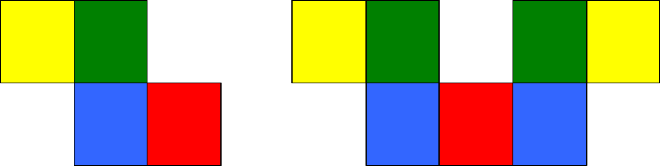
Figure 2: Model ${\cal M}_{1}$.

Example 1

In Figure 2 a quasi-discrete closure model ${\cal M}_{1}=((X_{1},{\cal C}_{R_{1}}),{\cal V}\,_{\!1})$ is shown where $X_{1}$ contains 11 elements, each represented by a coloured square box, which we call a cell. The relation $R_{1}$ is the so-called orthogonal adjacency relation [24], i.e. the reflexive and symmetric relation such that two cells are related iff they share an edge. Note, $X_{1}$ is not path-connected. The set $AP$ of atomic predicates is the set $\{\mathtt{red},\mathtt{blue},\mathtt{green},\mathtt{yellow}\}$ and ${\cal V}\,_{\!1}$ associates each predicate (i.e. colour) to the set of cells of that specific colour; in this example, each cell satisfies exactly one atomic proposition. The two red cells are $\,\cong_{{\cal C}}^{{\cal M}_{1}\!\!}-$bisimilar. In order to see this, consider the relation $B_{1}$ which is the minimal reflexive and symmetric binary relation on $X_{1}$ such that

• the two red points are related;

• the blue (green, yellow, respectively) point of the left-hand component is related to each blue (green, yellow, respectively) point of the right-hand component.

It is easy to see that $B_{1}$ satisfies the conditions of Definition 4. For instance, the (forward and backward) closure of the left-hand side red cell contains only the cell itself and the blue adjacent one and, for each such cell, there is one in the right-hand side of the same colour and related to the former by $B_{1}$. Similarly, the closure of the right-hand side red cell contains only the cell itself and the two blue adjacent ones and, for each such cell, there is one in the left-hand side with the same colour and related to the former by $B_{1}$. Similar reasoning applies to all other pairs of $B_{1}$. Finally, the two red cell are related by bisimulation relation  $B_{1}$ and so they are bisimilar.

(a)

(b)

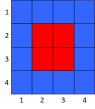
(c)

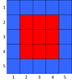
(d)

Figure 3: Models ${\cal M}_{a}$ (a), ${\cal M}_{b}$ (b), ${\cal M}_{c}$ (c), and ${\cal M}_{d}$ (d).

Example 2

For the sake of exposition, in this example, we will use matrix notation for referring to cells in Figure 3. Thus, $a_{2}$ and $b_{22}$ refer to the red cells in Figure 3(a) and 3(b), respectively, whereas the four red cells in Figure 3(c) are referred to as $c_{22},c_{23},c_{32},c_{33}$ and so on. We consider four models ${\cal M}_{j}=((X_{j},{\cal C}_{R_{j}}),{\cal V}\,_{\!j})$, for $j=a,b,c,d$. with $X_{a}=\{\,a_{i}\mid 1\leqslant i\leqslant 3\,\}$, $X_{b}=\{\,b_{ij}\mid 1\leqslant i,j\leqslant 3\,\}$, $X_{c}=\{\,c_{ij}\mid 1\leqslant i,j\leqslant 4\,\}$, $X_{d}=\{\,d_{ij}\mid 1\leqslant i,j\leqslant 5\,\}$. Differently from Example 1, in each of the four models ${\cal M}_{j}$, we assume an orthodiagonal adjacency relation $R_{j}$, namely, the reflexive and symmetric relation such that two cells in ${\cal M}_{j}$ are related iff they share an edge or a vertex [24]. For instance, $\{(c_{11},c_{12}),(c_{11},c_{22})\}\subseteq R_{c}$. This choice of the adjacency relation simplifies the description of the example. The set $AP$ of atomic propositions is the set $\{\mathtt{red},\mathtt{blue}\}$, with ${\cal V}\,_{\!a}\,\mathtt{red}=\{a_{2}\}$, ${\cal V}\,_{\!b}\,\mathtt{red}=\{b_{22}\}$, ${\cal V}\,_{\!c}\,\mathtt{red}=\bigcup_{i,j=2,2}^{3,3}\{c_{ij}\}$, and ${\cal V}\,_{\!d}\,\mathtt{red}=\bigcup_{i,j=2,2}^{4,4}\{d_{ij}\}$, with ${\cal V}\,_{\!j}\,\mathtt{blue}=X_{j}\setminus({\cal V}\,_{\!j}\,\mathtt{red})$ for $j\in\{a,b,c,d\}$. We use the shorthand $\gamma\mkern 1.0mux={\cal V}^{\mbox{\,\scriptsize--1}}_{j}\mkern 1.0mux$ for $x\in X_{j}$ and $j=a,b,c,d$. Note, since $R_{j}$ is reflexive, $\gamma\mkern 1.0mux$ includes the point $x$ itself. Moreover, the relations $B_{j}$ are defined as $B_{j}=\{\,(x,y)\in X_{j}^{2}\mid\gamma\mkern 1.0mux=\gamma\mkern 1.0muy\,\}$, for $j\in\{a,b,c\}$.

Clearly $a_{1}\,\simeq_{{\cal C}}^{{\cal M}_{a}}a_{3}$ since $(a_{1},a_{3})\in B_{a}$, which is a bisimulation. Take for instance ${\cal C}_{R_{a}}\mkern 1.0mu\!a_{1}=\{a_{1},a_{2}\}$ and note that $(a_{1},a_{3})\in B_{a}$ with $a_{3}\in{\cal C}_{R_{a}}\mkern 1.0mu\!a_{3}$ and, similarly, $(a_{2},a_{2})\in B_{a}$ with $a_{2}\in{\cal C}_{R_{a}}\mkern 1.0mu\!a_{3}$. The reasoning for the other cells of $X_{a}$ is similar.

It is also easy to see that for all $x,y\in X_{b}$ we have $x\,\simeq_{{\cal C}}^{{\cal M}_{b}}y$ iff $\gamma\mkern 1.0mux=\gamma\mkern 1.0muy$; for instance, for each element $z_{1}$ of ${\cal C}_{R_{b}}\mkern 1.0mub_{11}=\{b_{11},b_{12},b_{21},b_{22}\}$ there exists an element $z_{2}$ of ${\cal C}_{R_{b}}\mkern 1.0mub_{23}=\{b_{12},b_{13},b_{22},b_{23},b_{32},b_{33}\}$ such that $(z_{1},z_{2})\in B_{b}$, which is a bisimulation containing also $(b_{11},b_{23})$.

Let us now consider the model ${\cal M}_{ab}=((X_{a}\cup X_{b},{\cal C}_{(R_{a}\cup R_{b})}),{\cal V}\,_{\!ab})$ where ${\cal V}\,_{\!ab}\,p={{\cal V}\,_{\!a}\mkern 1.0mup}\mkern 1.0mu\cup\mkern 1.0mu{{\cal V}\,_{\!b}\mkern 1.0mup}$. We define the relation $B_{ab}\subseteq(X_{a}\cup X_{b})$ by $B_{ab}=\{\,(x,y)\in X_{a}\cup X_{b}\mid\gamma\mkern 1.0mux=\gamma\mkern 1.0muy\,\}$. The reader is invited to prove that $a_{2}\,\simeq_{{\cal C}}^{{\cal M}_{ab}}b_{22}$. Similar reasoning shows that $B_{c}$ is a bisimulation for ${\cal M}_{c}$ and that the quotient $X_{c/\!\!\,\simeq_{{\cal C}}^{{\cal M}_{c}}}=\{\{\,x\in X_{c}\mid\gamma\mkern 1.0mux=\mathtt{red}\,\},\{\,x\in X_{c}\mid\gamma\mkern 1.0mux=\mathtt{blue}\,\}\}$ is a two-element set. Also, for model ${\cal M}_{bc}=(((X_{b}\cup X_{c}),{\cal C}_{R_{b}\cup R_{c}}),{\cal V}\,_{\!bc})$, with ${\cal V}\,_{\!bc}\mkern 1.0mup={\cal V}\,_{\!b}\mkern 1.0mup\cup{\cal V}\,_{\!c}\mkern 1.0mup$, we have $c_{ij}\,\simeq_{{\cal C}}^{{\cal M}_{bc}}b_{22}$ for $i,j\in\{2,3\}$, due to the existence of the bisimulation $B_{bc}=\{\,(x,y)\in X_{b}\cup X_{c}\mid\gamma\mkern 1.0mux=\gamma\mkern 1.0muy\,\}$.

In general, if we take as a model the union ${\cal M}_{abc}$ of ${\cal M}_{a}$, ${\cal M}_{b}$ and ${\cal M}_{c}$, i.e. ${\cal M}_{abc}=(((X_{a}\cup X_{b}\cup X_{c})),{\cal C}_{R_{a}\cup R_{b}\cup R_{c}},{\cal V}\,_{\!abc})$, with ${\cal V}\,_{\!abc}\mkern 1.0mup={\cal V}\,_{\!a}\mkern 1.0mup\cup{\cal V}\,_{\!b}\mkern 1.0mup\cup{\cal V}\,_{\!c}\,p$, we can easily see that all blue cells are bisimilar to one another and all red cells are bisimilar to one another (and no blue cell is bisimilar to any red one). In fact, as hinted above, there exists a minimal model with just two cells, one red and one blue, that are adjacent (in this case, the orthogonal and the orthodiagonal relations coincide); all red (blue, respectively) cells of ${\cal M}_{abc}$ are equivalent to the red (blue, respectively) cell of the minimal model.

Finally, let us consider cell $d_{33}$ and, say, $d_{22}$ in model ${\cal M}_{d}$. It is easy to see that $d_{22}\not\,\simeq_{{\cal C}}^{{\cal M}_{d}}d_{33}$. In fact, ${\cal C}_{R_{d}}\mkern 1.0mud_{33}=\{\,x\in X_{d}\mid\gamma\mkern 1.0mux=\mathtt{red}\,\}$ and there is $y\in{\cal C}_{R_{d}}\mkern 1.0mud_{22}$ such that $\gamma\,y=\mathtt{blue}$. Thus, any bisimulation $B$ should include $(y,z)$ with $z\in{\cal C}_{R_{d}}\mkern 1.0mud_{33}$, because of the transfer condition 2 of Definition 4 with respect to $(d_{22},d_{33})$, but this is impossible because $(y,z)\in B$ would violate condition 3 of Definition 4 because $\gamma\mkern 1.0muy=\mathtt{blue}\neq\mathtt{red}=\gamma\mkern 1.0muz$.

4 Quasi-discrete Closure Models Coalgebraically

Let the quasi-discrete closure model ${\cal M}=((X,{\cal C}),{\cal V}\,)$ be finitely closed and finitely backward closed (but not necessarily finite). We can represent ${\cal M}$ as a pair $(X,\eta_{{\cal M}})$, with the function $\eta_{{\cal M}}:X\to(\mathcal{P}_{\omega}AP)\times(\mathcal{P}_{\omega}X)\times(\mathcal{P}_{\omega}X)$ such that $\eta_{{\cal M}}x=({\cal V}^{\mbox{-}\mkern-2.0mu\mbox{\scriptsize 1}}\mkern-1.5mux,\stackrel{{\scriptstyle\rightarrow}}{{{\cal C}}}\!\!x,\stackrel{{\scriptstyle\leftarrow}}{{{\cal C}}}\!\!x)$. In the sequel we will write $\eta$ instead of $\eta_{{\cal M}}$, when this does not cause confusion. Note that not all pairs $(X,\eta)$ represent closure models, but only those for which $(\eta\,x)_{3}=\{\,x^{\prime}\in X\mid x\in(\eta x^{\prime})_{2}\,\}$ and $(\eta\,x)_{2}=\{\,x^{\prime}\in X\mid x\in(\eta x^{\prime})_{3}\,\}$.

Example 3

Model ${\cal M}_{a}$ of Figure 3 corresponds to the pair $(\{a_{1},a_{2},a_{3}\},\eta_{a})$ with $\eta_{a}\,a_{1}=(\{\mathtt{blue}\},\{a_{1},a_{2}\},\{a_{1},a_{2}\})$, $\eta_{a}\,a_{2}=(\{\mathtt{red}\},\{a_{1},a_{2},a_{3}\},\{a_{1},a_{2},a_{3}\})$, and $\eta_{a}\,a_{3}=(\{\mathtt{blue}\},\{a_{2},a_{3}\},\{a_{2},a_{3}\})$. The other models of the figure can be represented similarly.

The following is a reformulation of bisimilarity in terms of the function $\eta_{{\cal M}}$.

Definition 6

An equivalence relation $B\subseteq X\times X$ is an $\eta$-bisimulation if $(x_{1},x_{2})\in B$ implies that the following holds:

1. $(\eta\,x_{1})_{1}=(\eta\,x_{2})_{1}$, and

2. for all $C\in X/B$ it holds that

   1. $(\eta\,x_{1})_{2}\cap C\not=\emptyset\mbox{ iff }(\eta\,x_{2})_{2}\cap C\neq\emptyset$, and

   2. $(\eta\,x_{1})_{3}\cap C\neq\emptyset\mbox{ iff }(\eta\,x_{2})_{3}\cap C\neq\emptyset.$

We say that $x_{1}$ and $x_{2}$ are $\eta$-bisimilar, notation $x_{1}\,\simeq_{\eta}\,x_{2}$, if there exists an $\eta$-bisimulation relation $B$ such that $(x_{1},x_{2})\in B$.

Example 4

With reference to model ${\cal M}_{a}$ of Figure 3 and $(\{a_{1},a_{2},a_{3}\},\eta_{a})$ above, it is easy to see that $a_{1}$ and $a_{3}$ are $\eta_{a}$-bisimilar.

The following lemma follows directly from Definition 5 and Definition 6.

Lemma 1

$\,\simeq_{\eta}\,$ coincides with $\,\simeq_{{\cal C}}$.

Definition 7

The functor ${\cal T}:\textbf{Set}\to\textbf{Set}$ assigns to a set $X$ the product set $\mathcal{P}_{\omega}AP\times\mathcal{P}_{\omega}X\times\mathcal{P}_{\omega}X$ and to a mapping $f:X\to Y$ the mapping ${\cal T}\mkern 1.0muf:(\mathcal{P}_{\omega}AP\to\mathcal{P}_{\omega}X\to\mathcal{P}_{\omega}X)\to(\mathcal{P}_{\omega}AP\times\mathcal{P}_{\omega}Y\times\mathcal{P}_{\omega}Y)$ where, for all $v\in\mathcal{P}_{\omega}AP$ and $z,z^{\prime}\in\mathcal{P}_{\omega}X$, $({\cal T}f)\mkern 1.0muv\mkern 1.0muz\mkern 1.0muz^{\prime}=(v,(fz),(fz^{\prime}))$.

Clearly, the model ${\cal M}$, represented as $(X,\eta)$, can be interpreted as a coalgebra of functor ${\cal T}$.

Lemma 2

The functor ${\cal T}$ has a final coalgebra.

Proof

Constants, finite products, and the finite powerset are $\omega$-accessible functors. The class of $\kappa$-accessible functors for any $\kappa$ is closed with respect to composition, and $\kappa$-accessible functors have final coalgebras. ∎

We recall that two elements $x_{1},x_{2}$ of an ${\cal T}$-coalgebra ${\cal X}$ are behavioural equivalent if $[\![{x_{1}}]\!]^{{\cal X}}_{{\cal T}}=[\![{x_{2}}]\!]^{{\cal X}}_{{\cal T}}$, denoted $x_{1}\approx^{{{\cal X}}}_{{{\cal T}}}x_{2}$, where $[\![{\cdot}]\!]^{{\cal X}}_{{\cal T}}$ is the unique morphism from ${\cal X}$ to the final coalgebra of functor ${\cal T}$.

The following theorem shows that behavioural equivalence and $\eta$-bisimilarity coincide. The proof follows the same pattern as that of Theorem 4.3 in [22].

Theorem 4.1

Behavioural equivalence and $\eta$-bisimilarity coincide, i.e. $\approx_{{{\cal T}}}\,=\,\,\simeq_{\eta}\,$.

Proof

Let $x_{1},x_{2}\in X$. We first prove that ${x_{1}\,\simeq_{\eta}\,x_{2}}$ implies $x_{1}\approx_{{{\cal T}}}x_{2}$. So, assume ${x_{1}\,\simeq_{\eta}\,x_{2}}$. Let $B\subseteq X\times X$ be an $\eta$-bisimulation with $(x_{1},x_{2})\in B$ and recall that $(X,\eta)$ is a ${\cal T}$-coalgebra. We turn the collection of equivalence classes $X/B$ into a ${\cal T}$-coalgebra ${\cal M}/B=(X/B,\varrho_{B})$ where, for $s\in X$

$$\varrho_{B}\,[s]_{B}=((\eta\mkern 1.0mus)_{1},\{\,C\in X/B\mid(\eta\mkern 1.0mus)_{2}\cap C\neq\emptyset\,\},\{\,C\in X/B\mid(\eta\mkern 1.0mus)_{3}\cap C\neq\emptyset\,\})$$

This is well-defined since $B$ is an $\eta$-bisimulation: if $(s,s^{\prime})\in B$ then we have

$$\begin{array}[]{rcll}\varrho_{B}\mkern 1.0mu[s]_{B}&=&((\eta\mkern 1.0mus)_{1},\{\,C\in X/B\mid(\eta\mkern 1.0mus)_{2}\cap C\neq\emptyset\,\},\{\,C\in X/B\mid(\eta\mkern 1.0mus)_{3}\cap C\neq\emptyset\,\})\\ &&\qquad\text{(def.\ of $\varrho_{B}$)}\\ &=&((\eta\mkern 1.0mus^{\prime})_{1},\{\,C\in X/B\mid(\eta\mkern 1.0mus^{\prime})_{2}\cap C\neq\emptyset\,\},\{\,C\in X/B\mid(\eta\mkern 1.0mus^{\prime})_{3}\cap C\neq\emptyset\,\})\\ &&\qquad\text{($(s,s^{\prime})\in B$; $B$ is an $\eta$-bisimulation)}\\ &=&\varrho_{B}\,[s^{\prime}]_{B}\qquad\text{(def.\ of $\varrho_{B}$).}\end{array}$$

The canonical mapping $\varepsilon_{B}:X\to X/B$ is a ${\cal T}$-homomorphism, i.e. $({\cal T}\,\varepsilon_{B})\mathop{\raisebox{0.5pt}{\scriptsize$\circ$}}\eta=\varrho_{B}\mathop{\raisebox{0.5pt}{\scriptsize$\circ$}}\varepsilon_{B}$ as can be verified as follows. For $s\in X$, we have

$$\begin{array}[]{rcll}({\cal T}\,\varepsilon_{B})(\eta\mkern 1.0mus)&=&((\eta\mkern 1.0mus)_{1},\varepsilon_{B}\mkern 1.0mu(\eta\mkern 1.0mus)_{2},\varepsilon_{B}\mkern 1.0mu(\eta\mkern 1.0mus)_{3})&\text{(def.\ of ${\cal T}$)}\\ &=&((\eta\mkern 1.0mus)_{1},\{\,[t]_{B}\mid t\in(\eta\mkern 1.0mus)_{2}\,\},\{\,[t]_{B}\mid t\in(\eta\mkern 1.0mus)_{3}\,\})\qquad\mbox{}&\text{(def.\ of $\varepsilon_{B}$)}\\ &=&\lx@intercol((\eta\mkern 1.0mus)_{1},\{\,C\in X/B\mid(\eta\mkern 1.0mus)_{2}\cap C\neq\emptyset\,\},\{\,C\in X/B\mid(\eta\mkern 1.0mus)_{3}\cap C\neq\emptyset\,\})\hfil\lx@intercol\\ &=&\varrho_{B}[s]_{B}&\text{(def.\ of $\varrho_{B}$)}\\ &=&\varrho_{B}(\varepsilon_{B}\,s)&\text{(def.\ of $\varepsilon_{B}$).}\end{array}$$

Thus, $({\cal T}\,\varepsilon_{B})\mathop{\raisebox{0.5pt}{\scriptsize$\circ$}}\eta=\varrho_{B}\mathop{\raisebox{0.5pt}{\scriptsize$\circ$}}\varepsilon_{B}$, i.e. $\varepsilon_{B}$ is a ${\cal T}$-homomorphism. Therefore, by uniqueness of a final morphism, we have $[\![{\cdot}]\!]^{{\cal M}}_{{\cal T}}=[\![{\cdot}]\!]^{{{\cal M}_{B}}}_{{\cal T}}\mathop{\raisebox{0.5pt}{\scriptsize$\circ$}}\,\varepsilon_{B}$. In particular, with respect to ${\cal M}$, this implies $[\![{x_{1}}]\!]^{{\cal M}}_{{\cal T}}=[\![{x_{2}}]\!]^{{\cal M}}_{{\cal T}}$ since $(x_{1},x_{2})\in B$ and so $(\varepsilon_{B}\,x_{1})=(\varepsilon_{B}\,x_{2})$. Thus, $x_{1}\approx_{{{\cal T}}}x_{2}$.

For the reverse—i.e. ${x_{1}\approx_{{{\cal T}}}x_{2}}$ implies ${x_{1}\,\simeq_{\eta}\,x_{2}}$—assume $x_{1}\approx_{{{\cal T}}}x_{2}$, i.e. $[\![{x_{1}}]\!]^{{\cal M}}_{{\cal T}}=[\![{x_{2}}]\!]^{{\cal M}}_{{\cal T}}$, for $x_{1},x_{2}\in X$. Define the relation $R\subseteq X\times X$ such that $(x_{1},x_{2})\in R$ iff $[\![{x_{1}}]\!]^{{\cal M}}_{{\cal T}}=[\![{x_{2}}]\!]^{{\cal M}}_{{\cal T}}$. We first show that $R$ is an $\eta$-bisimulation. Suppose $(s^{\prime},s^{\prime\prime})\in R$ and recall that $[\![{\cdot}]\!]^{{\cal M}}_{{\cal T}}:(X,\eta)\to(\Omega,\omega)$ is a ${\cal T}$-homomorphism. For what concerns the first condition of Definition 6 we have

$$\begin{array}[]{rcll}(\eta\mkern 1.0mus^{\prime})_{1}&=&(({\cal T}\,[\![{\cdot}]\!]_{{\cal T}})(\eta\,s^{\prime}))_{1}&\text{(def.\ of ${\cal T}$)}\\ &=&((({\cal T}\,[\![{\cdot}]\!]_{{\cal T}})\mathop{\raisebox{0.5pt}{\scriptsize$\circ$}}\eta)\,s^{\prime})_{1}\\ &=&((\omega\mathop{\raisebox{0.5pt}{\scriptsize$\circ$}}[\![{\cdot}]\!]_{{\cal T}})s^{\prime})_{1}&\text{($[\![{\cdot}]\!]_{{\cal T}}:(X,\eta)\to(\Omega,\omega)$ is homomorphism.)}\\ &=&(\omega\,[\![{s^{\prime}}]\!]_{{\cal T}})_{1}\\ &=&(\omega\,[\![{s^{\prime\prime}}]\!]_{{\cal T}})_{1}&\text{($[\![{s^{\prime}}]\!]_{{\cal T}}=[\![{s^{\prime\prime}}]\!]_{{\cal T}}$ since $(s^{\prime},s^{\prime\prime})\in R$)}\\ &=&((\omega\mathop{\raisebox{0.5pt}{\scriptsize$\circ$}}[\![{\cdot}]\!]_{{\cal T}})s^{\prime\prime})_{1}\\ &=&((({\cal T}\,[\![{\cdot}]\!]_{{\cal T}})\mathop{\raisebox{0.5pt}{\scriptsize$\circ$}}\eta)\,s^{\prime\prime})_{1}&\text{($({\cal T}\,[\![{\cdot}]\!]_{{\cal T}})\mathop{\raisebox{0.5pt}{\scriptsize$\circ$}}\eta=\omega\mathop{\raisebox{0.5pt}{\scriptsize$\circ$}}[\![{\cdot}]\!]_{{\cal T}}$)}\\ &=&(({\cal T}\,[\![{\cdot}]\!]_{{\cal T}})(\eta\,s^{\prime\prime}))_{1}\\ &=&(\eta\mkern 1.0mus^{\prime\prime})_{1}&\text{(def.\ of ${\cal T}$).}\end{array}$$

For what concerns the second condition of Definition 6 we have, for $h\in\{2,3\}$ and all $C\in X/R$, that

$$\begin{array}[]{rcll}\lx@intercol(\eta\mkern 1.0mus^{\prime})_{h}\cap C\neq\emptyset\hfil\lx@intercol\\ \mbox{\qquad}&\Leftrightarrow&(\eta\,s^{\prime})_{h}\cap[\![{w}]\!]^{-1}_{{\cal T}}\neq\emptyset\mbox{\qquad}&\\ &&\lx@intercol\qquad\text{(def.\ of ${[\![{\cdot}]\!]^{-1}_{{\cal T}}}$; def.\ of~{}$R$; $w=[\![{t}]\!]_{{\cal T}}$ for all $t\in C$)}\hfil\lx@intercol\\ &\Leftrightarrow&w\in(\omega{[\![{s^{\prime}}]\!]_{{\cal T}}})_{h}&\text{(by Lemma~{}\ref{lemma:aux} below)}\\ &\Leftrightarrow&w\in(\omega{[\![{s^{\prime\prime}}]\!]_{{\cal T}}})_{h}&\text{($[\![{s^{\prime}}]\!]_{{\cal T}}=[\![{s^{\prime\prime}}]\!]_{{\cal T}}$ since $(s^{\prime},s^{\prime\prime})\in R$)}\\ &\Leftrightarrow&(\eta\mkern 1.0mus^{\prime\prime})_{h}\cap[\![{w}]\!]^{-1}_{{\cal T}}\neq\emptyset&\text{(by Lemma~{}\ref{lemma:aux} below)}\\ &\Leftrightarrow&(\eta\mkern 1.0mus^{\prime\prime})_{h}\cap C\neq\emptyset\\ &&\lx@intercol\qquad\text{(def.\ of ${[\![{\cdot}]\!]^{-1}_{{\cal T}}}$; def.\ of~{}$R$; $w=[\![{t}]\!]_{{\cal T}}$ for all $t\in C$)}.\hfil\lx@intercol\end{array}$$

Since both conditions of Definition 6 are fulfilled, $R$ is an $\eta$-bisimulation relation and hence, since $(x_{1},x_{2})\in R$, we get ${x_{1}\,\simeq_{\eta}\,x_{2}}$. This completes the proof. ∎

In the proof of Theorem 4.1 we have made use of the following result.

Lemma 3

For $h\in\{2,3\}$, all $s\in X,w\in\Omega$ we have that $w\in(\omega\,{[\![{s}]\!]_{{\cal T}}})_{h}$ if and only if $(\eta\,s)_{h}\cap[\![{w}]\!]^{-1}_{{\cal T}}\not=\emptyset$.

Proof

See Appendix 0.A.

From Theorem 4.1 and Lemma 1 we get complete correspondence of behavioural equivalence and bisimilarity for quasi-discrete closure models .

Corollary 1

Given a quasi-discrete closure model ${\cal M}=((X,{\cal C}_{R}),{\cal V})$ based on $R$, for all $x_{1},x_{2}\in X$ it holds that $x_{1}\,\simeq_{{\cal C}}^{{\cal M}}x_{2}$ iff $x_{1}\approx^{{{\cal M}}}_{{{\cal T}}}x_{2}$.

Example 5

With reference to Example 2, we see that the minimal coalgebra for the models ${\cal M}_{a},{\cal M}_{b}$ and ${\cal M}_{c}$ is represented by $(\{\tau_{1},\tau_{2}\},\mu)$ where $\mu\mkern 1.0mu\tau_{1}=(\mathtt{blue},\{\tau_{1},\tau_{2}\},\{\tau_{1},\tau_{2}\})$, and $\mu\mkern 1.0mu\tau_{2}=(\mathtt{red},\{\tau_{1},\tau_{2}\},\{\tau_{1},\tau_{2}\})$. The quotient morphisms are the obvious ones; for instance, letting model ${\cal M}_{c}$ be represented by the coalgebra $(X_{c},\eta_{c})$, $h_{c}:(X_{c},\eta_{c})\to((\tau_{1},\tau_{2}),\mu)$ maps $c_{22},c_{23},c_{32}$, and $c_{33}$ to $\tau_{2}$, and all other elements to $\tau_{1}$. The minimal coalgebra for ${\cal M}_{d}$ is $(\{\tau_{3},\tau_{4},\tau_{5}\},\nu)$, where $\nu\mkern 1.0mu\tau_{3}=(\mathtt{red},\{\tau_{3},\tau_{4}\},\{\tau_{3},\tau_{4}\})$, $\nu\mkern 1.0mu\tau_{4}=(\mathtt{red},\{\tau_{3},\tau_{4},\tau_{5}\},\{\tau_{3},\tau_{4},\tau_{5}\})$, and $\nu\mkern 1.0mu\tau_{5}=(\mathtt{blue},\{\tau_{4},\tau_{5}\},\{\tau_{4},\tau_{5}\})$. The minimal models obtained using MiniLogicA are reported in Figure 4. Note that $h_{d}:(X_{d},\eta_{d})\to((\tau_{3},\tau_{4},\tau_{5}),\nu)$ maps $d_{33}$ to $\tau_{3}$, the elements of $\{\,d_{ij}\mid 2\leqslant i,j\leqslant 4\,\}\setminus\{d_{33}\}$ to $\tau_{4}$, and all the other elements to $\tau_{5}$. Finally, consider the union ${\cal M}_{abcd}$ of model ${\cal M}_{abc}$ and model ${\cal M}_{d}$. In this case, the minimal coalgebra is (isomorphic to) $(\{\tau_{1},\tau_{2},\tau_{3},\tau_{4},\tau_{5}\},\mu+\nu)$ where $(\mu+\nu)\mkern 1.0mu\tau=\mu\mkern 1.0mu\tau$ if $\tau=\tau_{1},\tau_{2}$ and $(\mu+\nu)\mkern 1.0mu\tau=\nu\mkern 1.0mu\tau$ if $\tau=\tau_{3},\tau_{4},\tau_{5}$.

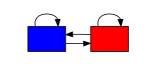
(a)

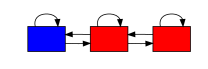
(b)

Figure 4: Minimal models obtained by running MiniLogicA on the images of Figure 3. Models ${\cal M}_{a},{\cal M}_{b}$ and ${\cal M}_{c}$ are all equivalent to the model on the left, whereas ${\cal M}_{d}$ is equivalent to the model on the right.

5 $\mathtt{SLCS}\$ and logical equivalence

We use the following version of the logic $\mathtt{SLCS}$ for a given set atomic propositions $AP$.

$$\Phi::=p\,\mid\,\neg\,\Phi\,\mid\,\Phi\,\lor\,\Phi\,\mid\,\mbox{\footnotesize${\stackrel{{\scriptstyle\rightarrow}}{{\rho}}}$}\,\Phi[\Phi]\,\mid\,\mbox{\footnotesize${\stackrel{{\scriptstyle\leftarrow}}{{\rho}}}$}\,\Phi[\Phi]$$ (1)

Satisfaction ${\cal M},x\models\Phi$ of a formula $\Phi$ at point $x\in X$ in a quasi-discrete closure model ${\cal M}=((X,{\cal C}_{R}),{\cal V}\,)$ is defined in Figure 5 by induction on the structure of formulas.

$\begin{array}[]{r c l c l c l l}{\cal M},x&\models&p\in P&\Leftrightarrow&x\in{\cal V}\,p\\ {\cal M},x&\models&\neg\,\Phi&\Leftrightarrow&{\cal M},x\models\Phi\mbox{ does not hold}\\ {\cal M},x&\models&\Phi_{1}\,\lor\,\Phi_{2}&\Leftrightarrow&{\cal M},x\models\Phi_{1}\mbox{ or }{\cal M},x\models\Phi_{2}\\ {\cal M},x&\models&\mbox{\footnotesize${\stackrel{{\scriptstyle\rightarrow}}{{\rho}}}$}\,\Phi_{1}[\Phi_{2}]&\Leftrightarrow&\mbox{there exists a path }\pi\mbox{ and an index }\ell\mbox{ such that }\\ &&&&\mbox{\hskip 7.22743pt}\pi(0)=x\,\mbox{ and }\,{\cal M},\pi(\ell)\models\Phi_{1}\mbox{ and }\\ &&&&\mbox{\hskip 7.22743pt}{\cal M},\pi(j)\models\Phi_{2},\mbox{ for all }j\mbox{ with }0<j<\ell\\ {\cal M},x&\models&\mbox{\footnotesize${\stackrel{{\scriptstyle\leftarrow}}{{\rho}}}$}\,\Phi_{1}[\Phi_{2}]&\Leftrightarrow&\mbox{there exists a path }\pi\mbox{ and an index }\ell\mbox{ such that }\\ &&&&\mbox{\hskip 7.22743pt}\pi(\ell)=x\,\mbox{ and }\,{\cal M},\pi(0)\models\Phi_{1}\mbox{ and }\\ &&&&\mbox{\hskip 7.22743pt}{\cal M},\pi(j)\models\Phi_{2},\mbox{ for all }j\mbox{ with }0<j<\ell\\ \end{array}$

Figure 5: Definition of the satisfaction relation

Some useful abbreviations are defined in Figure 6. The operator ${\cal N}$ is the near operator, namely the logical counterpart of the closure function of closure spaces: $x$ satisfies ${\cal N}\Phi$ iff it is “close” to $\Phi$, as defined in [14]. The operator ${\cal S}$ is the surrounded operator: a point $x$ satisfies $\Phi_{1}\,{\cal S}\,\Phi_{2}$ if it satisfies $\Phi_{1}$ and no path starting at $x$ can reach any point satisfying $\neg\,\Phi_{1}$ without first passing by a point satisfying $\Phi_{2}$, i.e. $x$ lays in an area that satisfies $\Phi_{1}$ and that is surrounded by points satisfying $\Phi_{2}$. The operator ${\cal P}$ is the propagation operator introduced in [14]: $x$ satisfies $\Phi_{1}\,{\cal P}\,\Phi_{2}$ if it satisfies $\Phi_{2}$ and it is reachable from a point satisfying $\Phi_{1}$ via a path such that all of its points, except possibly the starting point, satisfy $\Phi_{2}$. For more derived operators the reader is referred to [14].

Example 6

Consider Example 2. All the red points in Figure 3(a-c) satisfy ${\cal N}\,{\tt blue}$. The middle point in Figure 3(d) (point $d_{33}$) does not satisfy such formula, although it satisfies $\mbox{\footnotesize${\stackrel{{\scriptstyle\rightarrow}}{{\rho}}}$}\,\tt blue[\tt red]$.

$\begin{array}[]{l c l}\Phi_{1}\,\land\,\Phi_{2}&\equiv&\neg(\neg\Phi_{1}\,\lor\,\neg\Phi_{2})\\ \bot&\equiv&p\,\land\,\neg p\\ \top&\equiv&\neg\bot\\ {\cal N}\Phi&\equiv&\mbox{\footnotesize${\stackrel{{\scriptstyle\leftarrow}}{{\rho}}}$}\,\Phi[\bot]\\ \Phi_{1}\,{\cal S}\,\Phi_{2}&\equiv&\Phi_{1}\,\land\,\neg(\mbox{\footnotesize${\stackrel{{\scriptstyle\rightarrow}}{{\rho}}}$}\,\neg(\Phi_{1}\,\lor\,\Phi_{2})[\neg\Phi_{2}])\\ \Phi_{1}\,{\cal P}\,\Phi_{2}&\equiv&\Phi_{2}\land\mbox{\footnotesize${\stackrel{{\scriptstyle\leftarrow}}{{\rho}}}$}\,\Phi_{1}[\Phi_{2}]\end{array}$

Figure 6: Derived operators 

Definition 8

The $\mathtt{SLCS}$ equivalence relation with respect to model ${\cal M}$, namely $\simeq_{\mathtt{slcs}}^{{\cal M}}\subseteq X\times X$, is defined as follows: $x_{1}\simeq_{\mathtt{slcs}}^{{\cal M}}x_{2}$ iff for all $\mathtt{SLCS}$ formulas $\Phi$ we have that ${\cal M},x_{1}\models\Phi\Leftrightarrow{\cal M},x_{2}\models\Phi$.

In the following, for the sake of notational simplicity, we will write $\simeq_{\mathtt{slcs}}$ instead of $\simeq_{\mathtt{slcs}}^{{\cal M}}$ whenever this cannot cause confusion.

Lemma 4

If a quasi-discrete closure model ${\cal M}$ is finitely closed and finitely backward closed, then $\simeq_{\mathtt{slcs}}\,\subseteq\,\,\simeq_{{\cal C}}$.

Proof

See Appendix 0.A.

Lemma 5

If ${\cal M}$ is a quasi-discrete closure model, then $\,\simeq_{{\cal C}}\,\subseteq\,\simeq_{\mathtt{slcs}}$.

Proof

See Appendix 0.A.

Lemma 4 and Lemma 5 bring the following result.

Theorem 5.1

If closure model ${\cal M}=((X,{\cal C}),{\cal V}\,)$ is quasi-discrete, finitely closed, and finitely backward closed, then for all $x_{1},x_{2}\in X$, $x_{1}\,\,\simeq_{{\cal C}}\,x_{2}$ iff we have $x_{1}\,\simeq_{\mathtt{slcs}}\,x_{2}$.

Example 7

Let us provide formulas that uniquely characterise each of the points in Figure 4, proving that there are no different, bisimilar points in that figure, when it is considered as a single model by taking the disjoint union of the models (a) and (b). Let $\Phi_{1}={\tt blue}\land{\cal N}{\tt red}$, $\Phi_{2}={\tt red}\land{\cal N}{\tt blue}$, $\Phi_{3}={\tt red}\land\lnot{\cal N}{\tt blue}$. The blue point in Figure 4(a) is the only point satisfying $\Phi_{1}\land\lnot\mbox{\footnotesize${\stackrel{{\scriptstyle\rightarrow}}{{\rho}}}$}\,\Phi_{3}[\top]$. The red point in Figure 4(a) is the only point satisfying $\Phi_{2}\land\lnot{\cal N}\Phi_{3}$. The blue point in Figure 4(b) is the only point satisfying $\Phi_{1}\land\mbox{\footnotesize${\stackrel{{\scriptstyle\rightarrow}}{{\rho}}}$}\,\Phi_{3}[\top]$. The middle red point in Figure 4(b) is the only point satisfying $\Phi_{2}\land{\cal N}\Phi_{3}$. The rightmost red point in Figure 4(b) is the only point satisfying $\Phi_{3}$.

We close this section with a stronger version of Lemma 4, and consequently of Theorem 5.1. Let us consider the sub-logic $\mathtt{SLCS}^{-}$ of $\mathtt{SLCS}$ given by

$$\Phi::=p\,\mid\,\neg\,\Phi\,\mid\,\Phi\,\lor\,\Phi\,\mid\,\mbox{\footnotesize${\stackrel{{\scriptstyle\rightarrow}}{{\rho}}}$}\,\Phi[\bot]\,\mid\,\mbox{\footnotesize${\stackrel{{\scriptstyle\leftarrow}}{{\rho}}}$}\,\Phi[\bot]$$ (2)

and let $x_{1}\,\simeq_{\mathtt{slcs}^{-}}\,x_{2}$ denote the logical equivalence with respect to the sub-logic $\mathtt{SLCS}^{-}$.

Lemma 6 below lays the basis for showing that for two points $x_{1}$ and $x_{2}$ with $x_{1}\,\simeq_{\mathtt{slcs}^{-}}\,x_{2}$ also holds that $x_{1}\,\simeq_{\mathtt{slcs}}\,x_{2}$, i.e. using the full version $\mbox{\footnotesize${\stackrel{{\scriptstyle\rightarrow}}{{\rho}}}$}\,\Phi_{1}[\Phi_{2}]$ and $\mbox{\footnotesize${\stackrel{{\scriptstyle\leftarrow}}{{\rho}}}$}\,\Phi_{1}[\Phi_{2}]$ of the ${\stackrel{{\scriptstyle\rightarrow}}{{\rho}}}$ and ${\stackrel{{\scriptstyle\leftarrow}}{{\rho}}}$ operators does not add discriminatory power with respect to using the restricted versions $\mbox{\footnotesize${\stackrel{{\scriptstyle\rightarrow}}{{\rho}}}$}\,\Phi[\bot]$ and $\mbox{\footnotesize${\stackrel{{\scriptstyle\leftarrow}}{{\rho}}}$}\,\Phi[\bot]$.

Lemma 6

Formulas $\Phi_{1},\Phi_{2}$ of $\mathtt{SLCS}^{-}$ of Equation 2 satisfy the following.

1. If ${\cal M},x_{1}\models\mbox{\footnotesize${\stackrel{{\scriptstyle\rightarrow}}{{\rho}}}$}\,\Phi_{1}[\Phi_{2}]$ and ${\cal M},x_{2}\not\models\mbox{\footnotesize${\stackrel{{\scriptstyle\rightarrow}}{{\rho}}}$}\,\Phi_{1}[\Phi_{2}]$ then there exists $\Lambda_{\Phi_{1},\Phi_{2}}$ in the language of Equation 2 such that ${\cal M},x_{1}\models\Lambda_{\Phi_{1},\Phi_{2}}$ and ${\cal M},x_{2}\not\models\Lambda_{\Phi_{1},\Phi_{2}}$.

2. If ${\cal M},x_{1}\models\mbox{\footnotesize${\stackrel{{\scriptstyle\leftarrow}}{{\rho}}}$}\,\Phi_{1}[\Phi_{2}]$ and ${\cal M},x_{2}\not\models\mbox{\footnotesize${\stackrel{{\scriptstyle\leftarrow}}{{\rho}}}$}\,\Phi_{1}[\Phi_{2}]$ then there exists $\Lambda_{\Phi_{1},\Phi_{2}}$ in the language of Equation 2 such that ${\cal M},x_{1}\models\Lambda_{\Phi_{1},\Phi_{2}}$ and ${\cal M},x_{2}\not\models\Lambda_{\Phi_{1},\Phi_{2}}$.

Proof

See Appendix 0.A.

Using the above lemma, one can then prove the following result.

Theorem 5.2

If closure model ${\cal M}=((X,{\cal C}),{\cal V}\,)$ is quasi-discrete, finitely closing, and finitely backward closing, then for all $x_{1},x_{2}\in X$ we have $x_{1}\,\,\simeq_{{\cal C}}\,x_{2}$ iff $x_{1}\,\simeq_{\mathtt{slcs}^{-}}\,x_{2}$.

Remark 2

With reference to Remark 1 it is easy to see that while ${\cal M},x_{1}\models\mbox{\footnotesize${\stackrel{{\scriptstyle\leftarrow}}{{\rho}}}$}\,p[\bot]$, we have ${\cal M},x_{2}\not\models\mbox{\footnotesize${\stackrel{{\scriptstyle\leftarrow}}{{\rho}}}$}\,p[\bot]$.

6 A tool for spatial minimization

One of the major advantages of defining bisimilarity coalgebraically is the availability of the partition refinement algorithm, sometimes referred to as iteration along the final sequence (see e.g. [2]). In the category Set, the formulation of the algorithm is particularly simple and quite similar to classical results such as [20]. In Algorithm 1, we illustrate the algorithm. For $q$ a function, we let $\mathit{ker}(q)$ be its kernel, namely the partition of the domain induced by $q$.

1function minimizeRec ($\eta:X\to{\cal F}X$,$q:X\to{\cal F}^{k}\{*\}$)

2 let $q^{\prime}=({\cal F}q)\circ\eta$

3 if ($\mathit{ker}(q)=\mathit{ker}(q^{\prime})$) then

4  return $q$

5 else

6  return minimizeRec($\eta$,$q^{\prime}$)

7function minimize($\eta:X\to{\cal F}X$)

 return minimizeRec($\mathit{\eta}$,$\lambda x.*$)

Algorithm 1 The coalgebraic partition refinement algorithm in Set.

The function minimize accepts as input a ${\cal F}$-coalgebra $\eta$ and returns the bisimilarity quotient of its carrier set. Minimization is implemented via the function minimizeRec, which accepts as input the coalgebra map $\eta$, and a surjective function $q$, whose kernel is a partition of the carrier set. Such function is initialised to $\lambda x.*$, where $*$ is the only element of the singleton $\{*\}$, that is, the algorithm starts by assuming that all the elements of the carrier are bisimilar. The algorithm then applies one refinement step, by applying the functor ${\cal F}$ to $q$ and composing the result with $\eta$; this yields a new function $q^{\prime}=({\cal F}q)\circ\eta$. Note that such function is “almost always” surjective. Intuitively, at each iteration, function $q^{\prime}$ is obtained from $q$ by splitting the partitions induced by $q$ according to the “observations” that are obtained “in one more step” from $\eta$. If $q$ and $({\cal F}q)\circ\eta$ represent the same partition – that is, the two functions have the same kernel – the algorithm returns $q$, which denotes the coarsest partition that does not identify non-bisimilar states; otherwise, the procedure is iterated. Termination is guaranteed on finite models as for each finite model, there are only a finite number of partitions.

Algorithm 1, instantiated using the functor ${\cal T}$ of Section 4, has been implemented in a multi-platform tool called MiniLogicA, which is available for the major operating systems at https://github.com/vincenzoml/MiniLogicA under a permissive open source license. The tool is implemented in the language F#. The tool can load arbitrary (possibly directed) graphs, with explicit labelling of nodes with atomic propositions. Such labelled graphs are interpreted as quasi-discrete closure models. Additionally, the tool can load digital images, that are interpreted as symmetric, grid-shaped graphs, therefore as quasi-discrete models. More precisely, each pixel is interpreted as a node of a graph, and atomic propositions are derived from RGB colour components, whereas connectivity is derived from the union of the relations between pixels “have an edge in common” and “have a vertex in common” (in 2 dimensions, this corresponds to the classical orthodiagonal connectivity, that is, each non-border pixel is connected to 8 other pixels). The tool currently supports 2D images, but support of the same formats as VoxLogicA is planned. The tool outputs graphs in the graphviz format, with labels using atomic propositions, or colours according to the pixel colours of the input in the case of images.

7 Extension to Generic Closure Spaces

In this section we provide first a set-theoretic and next a coalgebraic notion of bisimilarity for closure models that aren’t necessarily quasi-discrete, and we prove that both coincide with logical equivalence as induced by an infinitary modal logic, here called IML, which, compared to $\mathtt{SLCS}$, does not include reachability operators. Instead, ${\cal N}\Phi$ is the basic operator—endowed with the classical closure semantics. Also, infinitary conjunction is allowed.

$$\Phi::=p\,\mid\,\neg\,\Phi\,\mid\,\textstyle{\bigwedge_{i\in I}}\>\Phi_{i}\,\mid\,{\cal N}\Phi$$ (3)

where $p\in AP$, and $I$ is a set.

For a closure model $((X,{\cal C}),{\cal V})$ we have, as expected, ${\cal M},x\models p$ $\Leftrightarrow$ $x\in{\cal V}p$, ${\cal M},x\models{\cal N}\Phi$ $\Leftrightarrow$ $x\in{\cal C}\mkern 1.0mu\{\,y\!\mid\!{\cal M},y\models\Phi\,\}$, ${\cal M},x\models\lnot\Phi$ $\Leftrightarrow$ ${\cal M},x\not\models\Phi$, and finally ${\cal M},x\models\bigwedge_{i\in I}\Phi_{i}$ $\Leftrightarrow$ ${\cal M},x\models\Phi_{i}$ for all $i\in I$.

Definition 9

The equivalence relation $\simeq_{\mathtt{IML}}^{{\cal M}}\subseteq X\times X$ is defined by $x_{1}\simeq_{\mathtt{IML}}^{{\cal M}}x_{2}$ iff for all IML formulas $\Phi$ we have that ${\cal M},x_{1}\models\Phi\Leftrightarrow{\cal M},x_{2}\models\Phi$.

In the sequel, $\simeq_{\mathtt{IML}}^{{\cal M}}$ will be often abbreviated by $\simeq_{\mathtt{IML}}$. The following definition extends the notion of bisimulation for topological spaces (see [9], for example) to general closure models.

Definition 10

Given a closure model ${\cal M}=((X,{\cal C}),{\cal V})$, a non-empty equivalence relation $B\subseteq X\times X$ is called a bisimulation relation if, for all $x_{1},x_{2}\in X$ such that $(x_{1},x_{2})\in B$, the next two conditions are satisfied.

1. ${\cal V}^{\mbox{-}\mkern-2.0mu\mbox{\scriptsize 1}}\mkern-1.5mux_{1}={\cal V}^{\mbox{-}\mkern-2.0mu\mbox{\scriptsize 1}}\mkern-1.5mux_{2}$.

2. For all $X_{1}\subseteq X$ such that $x_{1}\in{\cal I}\,X_{1}$, there is $X_{2}\subseteq X$ such that $x_{2}\in{\cal I}\,X_{2}$ and, reversely, for all $x_{2}^{\prime}\in X_{2}$ there exists $x_{1}^{\prime}\in X_{1}$ such that $(x_{1}^{\prime},x_{2}^{\prime})\in B$.

We say that $x_{1}$ and $x_{2}$ are bisimilar, notation $x_{1}\,\sim\,x_{2}$, if there exists a bisimulation relation $B$ for $X$ such that $(x_{1},x_{2})\in B$.

Remark 3

The definition of [9] (given for topological models) differs from the definition above in that the sets $X_{i}$ are required to be open neighbourhoods. In topology, a subset $S$ is an open neighbourhood of a point $x$ whenever there is an open set $O$ with $x\in O\subseteq S$, or, equivalently, $x\in{\cal I}\,S$. Therefore, in a topological space, Definition 10 coincides with the one of [9]. However, in general closure models, this is different. For instance consider a graph with three nodes $a,b,c$, and relation $R=\{(a,b),(b,c)\}$. Let $S=\{b,c\}$. We have ${\cal I}\,S=S\setminus{\cal C}\mkern 1.0mu\overline{S}=S\setminus{\cal C}\mkern 1.0mu\{a\}=S\setminus\{a,b\}=\{c\}\neq S$, therefore $S$ is not open (see also [14], Remark 2.19). Similarly, $\{c\}$ is not open as ${\cal I}\,\{c\}=\emptyset$. Thus $S$ does not include an open set containing $c$. However, $c\in{\cal I}\,S$.

Below, we show that logical equivalence in IML coincides with bisimilarity from Definition 10. The following two lemmas are required.

Lemma 7

For all $X_{1},X_{2}\subseteq X$, if $({\cal C}\mkern 1.0muX_{1})\cap({\cal I}\,X_{2})\neq\emptyset$ then $X_{1}\cap X_{2}\neq\emptyset$.

Proof

We prove that $X_{1}\cap X_{2}=\emptyset$ implies $({\cal C}\mkern 1.0muX_{1})\cap({\cal I}\,X_{2})=\emptyset$. Suppose $X_{1}\cap X_{2}=\emptyset$. Then $X_{1}\subseteq\overline{X}_{2}$, thus ${\cal C}\mkern 1.0muX_{1}\subseteq{\cal C}\mkern 1.0mu\overline{X}_{2}$. Since ${\cal I}\,X_{2}=\overline{{\cal C}\mkern 1.0mu(\overline{X}_{2})}$, it follows that $({\cal I}\,X_{2})\cap({\cal C}\mkern 1.0muX_{1})=\emptyset$. ∎

Lemma 8

For all $S\subseteq X$ and $y\in X$, if for all $C\subseteq X$ it holds that $y\in{\cal I}\,C$ implies $C\cap S\neq\emptyset$, then $y\in{\cal C}\mkern 1.0muS$.

Proof

By contradiction. Suppose $y\notin{\cal C}\mkern 1.0muS$ under the hypothesis of the lemma. Then $y\in\overline{{\cal C}\mkern 1.0muS}$, i.e. $y\in\overline{\overline{{\cal I}\,(\overline{S})}}={\cal I}\,(\overline{S})$. But then, by the hypothesis, taking $C=\overline{S}$ since $\overline{S}\subseteq X$, we would have that $\overline{S}\cap S\neq\emptyset$. ∎

With the two lemmas in place, we are in a position to prove the next results.

Theorem 7.1

Given a closure model ${\cal M}=((X,{\cal C}),{\cal V})$, any bisimulation $B$ according to Definition 10 is included in $\simeq_{\mathtt{IML}}^{\cal M}$.

Proof

By induction on the structure of $\Phi$. $\Phi={\cal N}\Phi^{\prime}$. Suppose $B$ is a bisimulation, $(x,y)\in B$ and, without loss of generality, ${\cal M},x\not\models\Phi$ and ${\cal M},y\models\Phi$. Let $F\subseteq X$ be the set of points satisfying $\Phi^{\prime}$. We have $y\in{\cal C}\mkern 1.0muF$ and $x\in\overline{{\cal C}\mkern 1.0muF}=\overline{\overline{{\cal I}\,(\overline{F})}}={\cal I}\,(\overline{F})$. Let $X_{1}=\overline{F}$. By $x\in{\cal I}\,X_{1}$, let $X_{2}$ be chosen according to Definition 10, with $y\in{\cal I}\,X_{2}$. By Lemma 7 we have $F\cap X_{2}\neq\emptyset$, since $y\in({\cal C}\mkern 1.0muF)\cap({\cal I}\,X_{2})$. Let $y^{\prime}\in F\cap X_{2}$. We have ${\cal M},y^{\prime}\models\Phi^{\prime}$, since $y^{\prime}\in F$. Since $B$ is a bisimulation according to Definition 10, there is $x^{\prime}\in X_{1}$ with $(x^{\prime},y^{\prime})\in B$. By the induction hypothesis ${\cal M},x^{\prime}\models\Phi^{\prime}$, thus $x^{\prime}\in F$, which contradicts $x^{\prime}\in X_{1}=\overline{F}$.

Theorem 7.2

Given model ${\cal M}=((X,{\cal C}),{\cal V})$, $\simeq_{\mathtt{IML}}^{\cal M}$ is a bisimulation according to Definition 10.

Proof

Suppose $x\simeq_{\mathtt{IML}}y$. Let $X_{1}$ be such that $x\in{\cal I}\,X_{1}$. Suppose there is no $X_{2}$ respecting the conditions of Definition 10. Then, either there is no $C\subseteq X$ such that $y\in{\cal I}\,C$ or for each such $C$ there is $y_{\mkern 1.0muC}\in C$ such that $x^{\prime}\simeq_{\mathtt{IML}}y_{\mkern 1.0muC}$ for no $x^{\prime}\in X_{1}$. In the first case we would have that, for all $C\subseteq X$, $y\notin\overline{{\cal C}\mkern 1.0mu(\overline{C})}$, i.e. $y\in{\cal C}\mkern 1.0mu(\overline{C})$. This would imply in turn that $y\in{\cal C}\mkern 1.0mu(\overline{X})=\emptyset$, which is absurd. In the second case, let $S$ be the set of all the $y_{\mkern 1.0muC}$ as above. We have $y\in{\cal C}\mkern 1.0muS$ by Lemma 8. For each $a\in X_{1}$ and $s\in S$, $a$ and $s$ are not logically equivalent: let $\Phi_{(a,s)}$ be a formula such that ${\cal M},a\not\models\Phi_{(a,s)}$ and ${\cal M},s\models\Phi_{(a,s)}$. Let $\Phi=\bigwedge_{\,s}\lnot\bigwedge_{\,a}\Phi_{(a,s)}$. We have that ${\cal M},x^{\prime}\models\Phi$ for all $x^{\prime}\in X_{1}$ and ${\cal M},y^{\prime}\not\models\Phi$ for all $y^{\prime}\in S$. To see the latter, observe that $\lnot\Phi=\bigvee_{\!s}\bigwedge_{\,a}\Phi_{(a,s)}$. For each $a$, each $y^{\prime}\in S$ satisfies at least $\bigwedge_{\,a}\Phi_{(a,y^{\prime})}$. Thus, we have a formula $\Phi$ with $X_{1}\subseteq F=\{\,z\in X\mid z\models\Phi\,\}$ and $S\subseteq\overline{F}$. By $x\in{\cal I}\,X_{1}$ and monotonicity of interior, we have $x\in{\cal I}\,F$, thus ${\cal M},x\models\lnot{\cal N}(\lnot\Phi)$. On the other hand, by $y\in{\cal C}\mkern 1.0muS$ and monotonicity of closure, we have $y\in{\cal C}\mkern 1.0mu(\overline{F})$, thus ${\cal M},y\models{\cal N}(\lnot\Phi)$, contradicting the hypothesis $x\simeq_{\mathtt{IML}}y$. ∎

The characterisation given by Definition 10 has the merit of extending the existing topological definition to closure spaces. However, in the setting of this paper it is worthwhile to investigate also a coalgebraic definition, which we do in the remainder of this section. Since our main objective is to characterise logical equivalence, we will not define frames, but just models, which we will call closure coalgebras.

Definition 11

A closure coalgebra is a coalgebra for the closure functor $\textbf{C}X=\mathcal{P}(AP)\times\mathcal{P}(\mathcal{P}X)$, where $\mathcal{P}-$ is the covariant powerset functor. The action of the functor on arrows maps $f:X\to Y$ to $\textbf{C}f:(\mathcal{P}(AP)\times\mathcal{P}(\mathcal{P}X))\to(\mathcal{P}(AP)\times\mathcal{P}(\mathcal{P}Y))$ such that $\textbf{C}f(v,S)=(v,\{(\mathcal{P}f)A|A\in S\})$.

We note in passing that a general coalgebraic treatment of modal logics – even the non-normal ones – can be done starting from neighbourhood frames [19], employing coalgebras for the functor $2^{2^{-}}$ (where $2^{-}$ is the contravariant power set functor). Our definition is similar, but in contrast we employ the covariant powerset functor $\mathcal{P}$, which we find particularly profitable, as the obtained theory is akin to the developments of Section 4. The remainder of this section is aimed at determining a correspondence between closure models, closure coalgebras, and their quotients.

Definition 12

Given a closure model $((X,{\cal C}),{\cal V})$, define the coalgebra $\eta:X\to\textbf{C}X$ by $\eta(x)=(\mkern 1.0mu{\cal V}^{\mbox{-}\mkern-2.0mu\mbox{\scriptsize 1}}{}x,\{\,A\subseteq X\mid x\in{\cal C}A\mkern 1.0mu\})$.

It is straightforward to check that if $f:{\cal X}\to{\cal Y}$ is a C-coalgebra homomorphism, and both ${\cal X}$ and ${\cal Y}$ have been obtained from closure models using Definition 12, then $f$ is a continuous function in the sense of Definition 2. From now on, we shall not rely on the existence of a final coalgebra, as this is not the case for the (unbounded) powerset functor. However, we can employ maximal quotients instead, for the purpose of this paper. Therefore, we will redefine behavioural equivalence from Section 2.

Definition 13

Given a set functor ${\cal F}$ and a ${\cal F}$-coalgebra ${\cal X}=(X,\alpha)$ with $\alpha:X\to{\cal F}X$, the relation $\approx^{{{\cal X}}}_{{{\cal F}}}$, defined by

$x\approx^{{{\cal X}}}_{{{\cal F}}}y\Leftrightarrow\exists{\cal Y}=(Y,\beta).\exists f:{\cal X}\to{\cal Y}.f(x)=f(y)$

is called behavioural equivalence.

In Definition 13 we use the word equivalence, but this should not be taken for granted, of course. Clearly, $\approx$ is reflexive and symmetric, but transitivity is in principle to be shown. However (see [21], Theorem 1.2.4) pushouts in a Set-based category of coalgebras exist and are computed in the base category, which immediately yields transitivity of $\approx$. It is also obvious that when a final coalgebra exists, $\approx$ coincides with the kernel of the final morphism from ${\cal X}$.

Lemma 9

Consider a model ${\cal M}=((X,{\cal C}_{X}),{\cal V})$ and ${\cal X}=(X,\eta)$ as in Definition 12. Let ${\cal Y}=(Y,\theta)$ be a C-coalgebra. Let $f:{\cal X}\twoheadrightarrow{\cal Y}$ be a surjective coalgebra homomorphism. Define ${\cal C}_{Y}\mkern 1.0mu(B\subseteq Y)=\{\,y\in Y\mid B\in(\theta y)_{2}\,\}$. Then $(Y,{\cal C}_{Y})$ is a closure space.

Proof

See Appendix 0.A.

The proof of Theorem 7.3 below requires the following lemma, whose proof crucially relies on the fact that $A\subseteq B$ implies ${\cal C}\mkern-2.0muA\subseteq{\cal C}B$.

Lemma 10

Let $f$ be the function mapping each element of $X$ into its equivalence class up to $\simeq_{\mathtt{IML}}$. Then it holds that $((x_{1}\simeq_{\mathtt{IML}}x_{2})\land x_{1}\in{\cal C}\mkern 1.0mu\mkern-2.0muA)$ implies $x_{2}\in{\cal C}f^{-1}(\mathcal{P}f)A$, for all $x_{1},x_{2}\in X$ and $A\subseteq X$.

Proof

See Appendix 0.A.

With Lemma 9 and Lemma 10 available, we arrive at the following result.

Theorem 7.3

Consider a closure model ${\cal M}=((X,{\cal C}),{\cal V})$ and ${\cal X}=(X,\eta)$, with $\eta$ as in Definition 12. It holds that the relations $\simeq_{\mathtt{IML}}^{{\cal M}}$ and $\approx^{{{\cal X}}}_{{\textbf{C}}}$ coincide.

Proof

First, let us prove that if we have ${\cal M},x_{1}\models\Phi\Leftrightarrow{\cal M},x_{2}\models\Phi$ for all $\Phi$ and $x_{1},x_{2}\in X$, then there are a coalgebra ${\cal Y}=(Y,\theta)$ and a coalgebra homomorphism $f:X\to Y$ with $fx_{1}=fx_{2}$. Let $Y$ be the set of equivalence classes of $X$ under $\simeq_{\mathtt{IML}}^{{\cal M}}$. Let $f$ be the canonical map, mapping each $x\in X$ to its equivalence class $[x]$ with respect to $\simeq_{\mathtt{IML}}^{{\cal M}}$. Note that each element of $Y$ is of the form $f\mkern-1.0mux$ for some $x$. Define $tx=\{\,(\mathcal{P}f)A\mid A\in(\eta x)_{2}\,\}$, and let $\theta(fx)=((\eta\mkern 1.0mux)_{1},t(x))$. Observe that such a definition makes $f$ a coalgebra homomorphism by construction, that is, $\theta\circ f=(\textbf{C}f)\circ\eta$. We need to show that the definition of $\theta$ is independent from the representative $x$, i.e. whenever $x_{1}\simeq_{\mathtt{IML}}x_{2}$, we have $\theta(fx_{1})=\theta(fx_{2})$. Indeed, it is obvious that $(\eta x_{1})_{1}=(\eta x_{2})_{1}$, since by logical equivalence $x_{1}$ and $x_{2}$ satisfy the same atomic propositions. We thus need to show that $t\,x_{1}=t\,x_{2}$. All elements of $t\,x_{1}$ are of the form $(\mathcal{P}f)A$ with $x_{1}\in{\cal C}_{X}\mkern 1.0mu\mkern-2.0muA$. By Lemma 10, we then have $x_{2}\in{\cal C}_{X}(f^{-1}(\mathcal{P}f)A)$, thus $f^{-1}((\mathcal{P}f)A)\in(\eta x_{2})_{2}$ by definition of $\eta$. Therefore, $(\mathcal{P}f)(f^{-1}(\mathcal{P}f)\mkern 0.0muA)\in tx_{2}$ by definition of $t$, and since $(\mathcal{P}f)f^{-1}((\mathcal{P}f)\mkern 0.0muA)=(\mathcal{P}f)\mkern 0.0muA$, we obtain $t\,x_{1}\subseteq t\,x_{2}$. The same reasoning can also be used in the other direction, proving that the two sets are equal.

Next, we shall prove that if $((X,{\cal C}_{X}),{\cal V}{})$ is a closure model, with corresponding C-coalgebra $(X,\eta)$, $({\cal Y},\theta)$ is a C-coalgebra, $f:X\to Y$ is a coalgebra homomorphism, and $fx_{1}=fx_{2}$, then we have that ${\cal M},x_{1}\models\Phi\iff{\cal M},x_{2}\models\Phi$ for all $\Phi$. We will actually prove a slightly stronger statement, based upon Lemma 9. Given that the category of C-coalgebras has a epi-mono factorization system inherited from Set (that is, each coalgebra homomorphism can be written as $m\circ e$ where $e$ is surjective and $m$ is injective), let us restrict, without loss of generality, to the case when $f$ is surjective. By Lemma 9, there is a closure operator ${\cal C}_{Y}$ such that ${\cal M}^{\prime}=((Y,{\cal C}_{Y}),\theta_{1})$ is a closure model. Therefore, we can also interpret formulas on points of $Y$. Once this is established, under the hypothesis that $f$ is a (surjective) homomorphism, we shall prove that for all $x\in X$, we have ${\cal M},x\models\Phi\iff{\cal M}^{\prime},fx\models\Phi$ for all $\Phi$. This entails the main thesis as follows: whenever $fx_{1}=fx_{2}$, for all $\Phi$, we have ${\cal M},x_{1}\models\Phi\iff{\cal M}^{\prime},fx_{1}\models\Phi\iff{\cal M}^{\prime},fx_{2}\models\Phi\iff{\cal M},x_{2}\models\Phi$. The proof proceeds by induction on the structure of $\Phi$. The relevant case is that for formulas of the form ${\cal N}\Phi$. The proof of this case is split into two directions. Below, for any $\Phi$, we denote by $S^{X}_{\Phi}$ the set $\{\,x\in X\mid{\cal M},x\models\Phi\,\}$ and with $S^{Y}_{\Phi}$ the set $\{\,y\in Y\mid{\cal M}^{\prime},y\models\Phi\,\}$.

($\Rightarrow$) If ${\cal M},x\models{\cal N}\Phi$, then $x\in{\cal C}_{X}S^{X}_{\Phi}$ by definition of satisfaction, hence $S^{X}_{\Phi}\in(\eta\mkern 1.0mux)_{2}$ by definition of $\eta$, thus $(\mathcal{P}f)S^{X}_{\Phi}\in(\theta fx)_{2}$ since $f$ is a coalgebra homomorphism, and therefore $fx\in{\cal C}_{Y}((\mathcal{P}f)S^{X}_{\Phi})$. Now observe that whenever $y\in(\mathcal{P}f)S^{X}_{\Phi}$, we have that $y=f\mkern-1.0mux$ and ${\cal M},x\models\Phi$ for some $x$. Therefore, by inductive hypothesis, ${\cal M}^{\prime},y\models\Phi$. In other words, $(\mathcal{P}f)S^{X}\Phi\subseteq S^{Y}_{\Phi}$. By properties of closure, we have ${\cal C}_{Y}\mkern 1.0mu((\mathcal{P}f)S^{X}\Phi)\subseteq{\cal C}_{Y}\mkern 1.0muS^{Y}_{\Phi}$. Thus, by the above derivation, we have $f\mkern-1.0mux\in{\cal C}_{Y}\mkern 1.0muS^{Y}_{\Phi}$, that is ${\cal M}^{\prime},fx\models{\cal N}\Phi$.

($\Leftarrow$) If ${\cal M}^{\prime},fx\models{\cal N}\Phi$, then $fx\in{\cal C}_{Y}\mkern 1.0muS^{Y}_{\Phi}$ by definition of $S^{Y}_{\Phi}$, hence $S^{Y}_{\Phi}\in(\theta fx)_{2}$ by definition of $\theta$, and $S^{Y}_{\Phi}\in((\textbf{C}f)(\eta\mkern 1.0mux))_{2}$ since $f$ is a coalgebra homomorphism. Thus $(\mathcal{P}f)A=S^{Y}_{\Phi}$ for some $A\in(\eta\mkern 1.0mux)_{2}$, hence $(\mathcal{P}f)A=S^{Y}_{\Phi}$ and $x\in{\cal C}_{X}\mkern 1.0muA$, from which it follows that ${\cal M}^{\prime},fx^{\prime}\models\Phi$ for all $x^{\prime}\in A$. By induction hypothesis, ${\cal M},x^{\prime}\models\Phi$ for all $x^{\prime}\in A$, hence $A\subseteq S^{X}_{\Phi}$ and ${\cal C}_{X}\mkern 1.0mu\mkern-2.0muA\subseteq{\cal C}_{X}\mkern 1.0mu\mkern-1.0muS^{X}_{\Phi}$ by monotonicity of closure. It follows that $x\in{\cal C}_{X}\mkern 1.0mu\mkern-1.0muS^{X}_{\Phi}$ and ${\cal M},x\models{\cal N}\Phi$, as was to be shown. ∎

8 Concluding Remarks

In the context of spatial logics and model checking for closure spaces, we have developed a coalgebraic definition of spatial bisimilarity, a minimization algorithm, and a free and open source minimisation tool. Bisimilarity characterises logical equivalence of a finitary logic with two spatial reachability operators. Furthermore, we have generalised the definition of topo-bismilarity from topological spaces to closure spaces, proving that the more general definition still behaves as topo-bisimilarity, in that it characterises equivalence of infinitary modal logic. Finally, we have provided a coalgebraic characterisation in the more general setting. Indeed, one of the primary motivations for our work is the expectation that the tool can be refined, and the implementation can be integrated with the state-of-the-art spatial model checker VoxLogicA, to improve its efficiency, especially when spatial structures are procedurally generated (e.g. by a graph rewriting procedure or by a process calculus). However, we can identify a number of theoretical questions, that have the potential to lead to interesting developments of the research line of spatial model checking.

One major issue that has not yet been addressed is a treatment of logics with reachability, in the more general setting of Section 7. One major difficulty here is that the notion of a path has not been defined in the literature for closure spaces; in [14] it was emphasized (see Section 2.4) that the well-known topological definition does not generalise in the expected way, as it is not compatible with another fundamental notion, that of paths in a finite graph. Identifying a general notion of path would allow us to interpret reachability operators in general closure spaces. Such development is not a merely theoretical exercise. We expect that there are classes of non-quasi-discrete spaces, that may be finitely represented. For instance, variants of the polyhedra-based approach of [10] may be relevant for dealing with Euclidean spaces, and in practical terms, for reasoning about 3D meshes that are of common use in Computer Graphics. Also spaces that are the union of different components, based either on polyhedra or on graphs, can give rise to a hybrid spatial model checking approach in the same vein as the celebrated results on model checking of hybrid systems in the temporal case (see [17]).

Future work should also be devoted to clarifying the generality of the notion of a closure coalgebra, and to provide a more thorough comparison of closure coalgebras and neighbourhood frames. In this context, it is also relevant to investigate the link between closure coalgebras and the treatment of monotone logics of [18], given that monotonicity of closure is used in both directions for the proof of Theorem 7.3.

Appendix 0.A Appendix: additional proofs

Lemma 3. For $h\in\{2,3\}$, all $s\in X,w\in\Omega$ we have that $w\in(\omega\,{[\![{s}]\!]_{{\cal T}}})_{h}$ if and only if $(\eta\,s)_{h}\cap[\![{w}]\!]^{-1}_{{\cal T}}\not=\emptyset$.

Proof

Since $[\![{\cdot}]\!]_{{\cal T}}$ is a ${\cal T}$-homomorphism, we can make the following derivation

$\noindent\hskip 14.45377pt\vspace{0.1in}(\omega\,[\![{s}]\!]_{{\cal T}})_{h}\newline =\hskip 18.06749pt\{$Def. of $\mathop{\raisebox{0.5pt}{\scriptsize$\circ$}}$$\}\vspace{0.1in}\newline \hskip 14.45377pt\vspace{0.1in}((\omega\mathop{\raisebox{0.5pt}{\scriptsize$\circ$}}[\![{\cdot}]\!]_{{\cal T}})s)_{h}\newline =\hskip 18.06749pt\{$$[\![{\cdot}]\!]_{{\cal T}}$ is a ${\cal T}$-homomorphism$\}\vspace{0.1in}\newline \hskip 14.45377pt\vspace{0.1in}((({\cal T}\,[\![{\cdot}]\!]_{{\cal T}})\mathop{\raisebox{0.5pt}{\scriptsize$\circ$}}\eta)s)_{h}\newline =\hskip 18.06749pt\{$Def. of $\mathop{\raisebox{0.5pt}{\scriptsize$\circ$}}$$\}\vspace{0.1in}\newline \hskip 14.45377pt\vspace{0.1in}(({\cal T}\,[\![{\cdot}]\!]_{{\cal T}})(\eta\,s))_{h}\newline =\hskip 18.06749pt\{$Def. of $({\cal T}\,[\![{\cdot}]\!]_{{\cal T}})$$\}\vspace{0.1in}\newline \hskip 14.45377pt\vspace{0.1in}[\![{(\eta\,s)_{h}}]\!]_{{\cal T}}$

So, $w\in(\omega\,[\![{s}]\!]_{{\cal T}})_{h}$ if and only if $w\in[\![{(\eta\,s)_{h}}]\!]_{{\cal T}}$. But $w\in[\![{(\eta\,s)_{h}}]\!]_{{\cal T}}$ if and only if there exists $s^{\prime}\in(\eta\,s)_{h}$ such that $w=[\![{s^{\prime}}]\!]_{{\cal T}}$, i.e. if and only if $s^{\prime}\in[\![{w}]\!]^{-1}_{{\cal T}}$. So, $w\in(\omega\,[\![{s}]\!]_{{\cal T}})_{h}$ if and only there exists $s^{\prime}\in(\eta\,s)_{h}\cap[\![{w}]\!]^{-1}_{{\cal T}}$.
This proves the assert. ∎

Lemma 4. If quasi-discrete closure model ${\cal M}$ is finite-closure and back-finite-closure, then $\simeq_{\mathtt{slcs}}\,\subseteq\,\,\simeq_{{\cal C}}$.

Proof

We prove that the equivalence relation $\simeq_{\mathtt{slcs}}$ is a bisimulation by showing that for all $(x_{1},x_{2})\in\simeq_{\mathtt{slcs}}$ the five conditions of Definition 4 are satisfied:

1. $(x_{1},x_{2})\in\simeq_{\mathtt{slcs}}$ implies ${\cal M},x_{1}\models p$ if and only if ${\cal M},x_{2}\models p$ for all $p\in AP$, which implies in turn that ${\cal V}^{\mbox{-}\mkern-2.0mu\mbox{\scriptsize 1}}\mkern-1.5mux_{1}={\cal V}^{\mbox{-}\mkern-2.0mu\mbox{\scriptsize 1}}\mkern-1.5mux_{2}$;

2. suppose there exists $x_{1}^{\prime}\in\stackrel{{\scriptstyle\rightarrow}}{{{\cal C}}}\!\!x_{1}$ such that $(x_{1}^{\prime},x_{2}^{\prime})\not\in\simeq_{\mathtt{slcs}}$ for all $x_{2}^{\prime}\in\stackrel{{\scriptstyle\rightarrow}}{{{\cal C}}}\!\!x_{2}$. Note that $x_{1}^{\prime}\not=x_{1}$ because $x_{2}\in\stackrel{{\scriptstyle\rightarrow}}{{{\cal C}}}\!\!x_{2}\not=\emptyset$ and $(x_{1},x_{2})\in\simeq_{\mathtt{slcs}}$; moreover $\stackrel{{\scriptstyle\rightarrow}}{{{\cal C}}}\!\!x_{2}$ is finite since ${\cal M}$ is finite-closure. Let then $\stackrel{{\scriptstyle\rightarrow}}{{{\cal C}}}\!\!x_{2}=\{y_{1},\ldots,y_{n}\}$, with $(x_{1}^{\prime},y_{i})\not\in\simeq_{\mathtt{slcs}}$, for $i=1\ldots n$. This implies that there would exist formulas $\Phi_{1},\ldots,\Phi_{n}$ such that ${\cal M},x_{1}^{\prime}\models\Phi_{i}$ and ${\cal M},y_{i}\not\models\Phi_{i}$, for $i=1\ldots n$, by definition of $\simeq_{\mathtt{slcs}}$. Thus we would have ${\cal M},x_{1}^{\prime}\models\bigwedge_{j=1}^{n}\Phi_{j}$ and ${\cal M},y_{i}\not\models\bigwedge_{j=1}^{n}\Phi_{j}$ for $i=1\ldots n$, which would imply ${\cal M},x_{1}\models\mbox{\footnotesize${\stackrel{{\scriptstyle\rightarrow}}{{\rho}}}$}\,(\bigwedge_{j=1}^{n}\Phi_{j})[\bot]$ and ${\cal M},x_{2}\not\models\mbox{\footnotesize${\stackrel{{\scriptstyle\rightarrow}}{{\rho}}}$}\,(\bigwedge_{j=1}^{n}\Phi_{j})[\bot]$, and this would contradict $(x_{1},x_{2})\in\simeq_{\mathtt{slcs}}$. Thus we get that for all $x_{1}^{\prime}\in\stackrel{{\scriptstyle\rightarrow}}{{{\cal C}}}\!\!x_{1}$ there exists $x_{2}^{\prime}\in\stackrel{{\scriptstyle\rightarrow}}{{{\cal C}}}\!\!x_{2}$ such that $(x_{1}^{\prime},x_{2}^{\prime})\in\simeq_{\mathtt{slcs}}$;

3. symmetric to the case above;

4. suppose there exists $x_{1}^{\prime}\in\stackrel{{\scriptstyle\leftarrow}}{{{\cal C}}}\!\!x_{1}$ such that $(x_{1}^{\prime},x_{2}^{\prime})\not\in\simeq_{\mathtt{slcs}}$ for all $x_{2}^{\prime}\in\stackrel{{\scriptstyle\leftarrow}}{{{\cal C}}}\!\!x_{2}$. Note that $x_{1}^{\prime}\not=x_{1}$ because $x_{2}\in\stackrel{{\scriptstyle\leftarrow}}{{{\cal C}}}\!\!x_{2}\not=\emptyset$ and $(x_{1},x_{2})\in\simeq_{\mathtt{slcs}}$; moreover $\stackrel{{\scriptstyle\leftarrow}}{{{\cal C}}}\!\!x_{2}$ is finite since ${\cal M}$ is finite-back-closure. Let then $\stackrel{{\scriptstyle\leftarrow}}{{{\cal C}}}\!\!x_{2}=\{y_{1},\ldots,y_{n}\}$, with $(x_{1}^{\prime},y_{i})\not\in\simeq_{\mathtt{slcs}}$, for $i=1\ldots n$. This implies that there would exist formulas $\Phi_{1},\ldots,\Phi_{n}$ such that ${\cal M},x_{1}^{\prime}\models\Phi_{i}$ and ${\cal M},y_{i}\not\models\Phi_{i}$, for $i=1\ldots n$, by definition of $\simeq_{\mathtt{slcs}}$. Thus we would have ${\cal M},x_{1}^{\prime}\models\bigwedge_{j=1}^{n}\Phi_{j}$ and ${\cal M},y_{i}\not\models\bigwedge_{j=1}^{n}\Phi_{j}$ for $i=1\ldots n$, which would imply ${\cal M},x_{1}\models\mbox{\footnotesize${\stackrel{{\scriptstyle\leftarrow}}{{\rho}}}$}\,(\bigwedge_{j=1}^{n}\Phi_{j})[\bot]$ and ${\cal M},x_{2}\not\models\mbox{\footnotesize${\stackrel{{\scriptstyle\leftarrow}}{{\rho}}}$}\,(\bigwedge_{j=1}^{n}\Phi_{j})[\bot]$, and this would contradict $(x_{1},x_{2})\in\simeq_{\mathtt{slcs}}$. Thus we get that for all $x_{1}^{\prime}\in\stackrel{{\scriptstyle\leftarrow}}{{{\cal C}}}\!\!x_{1}$ there exists $x_{2}^{\prime}\in\stackrel{{\scriptstyle\leftarrow}}{{{\cal C}}}\!\!x_{2}$ such that $(x_{1}^{\prime},x_{2}^{\prime})\in\simeq_{\mathtt{slcs}}$;

5. symmetric to the case above. ∎

Lemma 5. If ${\cal M}$ is a quasi-discrete closure model, then $\,\simeq_{{\cal C}}\,\subseteq\,\simeq_{\mathtt{slcs}}$.

The proof requires the following lemma.

Lemma 11

For all quasi-discrete models ${\cal M}=((X,{\cal C}_{R}),{\cal V}\,)$, formulas $\Phi$ and $\Psi$, and $x,x^{\prime}\in X$ the following holds:

1. if $x^{\prime}\in\stackrel{{\scriptstyle\rightarrow}}{{{\cal C}}}\!\!x$ and ${\cal M},x^{\prime}\models\Phi$ then ${\cal M},x\models\mbox{\footnotesize${\stackrel{{\scriptstyle\rightarrow}}{{\rho}}}$}\,\Phi[\Psi]$;

2. if $x^{\prime}\in\stackrel{{\scriptstyle\leftarrow}}{{{\cal C}}}\!\!x$ and ${\cal M},x^{\prime}\models\Phi$ then ${\cal M},x\models\mbox{\footnotesize${\stackrel{{\scriptstyle\leftarrow}}{{\rho}}}$}\,\Phi[\Psi]$.

Proof

(of Lemma 11) Keeping in mind that $Y\subseteq{\cal C}\mkern 1.0muY$ for all $Y\subseteq X$

1. take $\pi:\mathbb{N}\to X$ with $\pi(0)=x$ and $\pi(j)=x^{\prime}$ for all $j\in\mathbb{N},j>0$; $\pi$ is a path since for all $N\subseteq\mathbb{N}$ we have

   $$\pi({\cal C}_{Succ}\mkern 1.0muN)=\left\{\begin{array}[]{l}\emptyset,\mbox{ if }N=\emptyset,\\ \{x^{\prime}\},\mbox{ if }0\not\in N\not=\emptyset,\\ \{x,x^{\prime}\},\mbox{ if }0\in N.\end{array}\right.\quad{\cal C}_{R}\mkern 1.0mu\pi(N)=\left\{\begin{array}[]{l}\emptyset,\mbox{ if }N=\emptyset,\\ {\cal C}_{R}\mkern 1.0mu\{x^{\prime}\},\mbox{ if }0\not\in N\not=\emptyset,\\ {\cal C}_{R}\mkern 1.0mu\{x,x^{\prime}\},\mbox{ if }0\in N.\\ \end{array}\right.$$

   so that $\pi({\cal C}_{Succ}\mkern 1.0muN)\subseteq{\cal C}_{R}\mkern 1.0mu(\pi N)$;

2. note that if $x^{\prime}\in\stackrel{{\scriptstyle\leftarrow}}{{{\cal C}}}\!\!x$ then $x\in\stackrel{{\scriptstyle\rightarrow}}{{{\cal C}}}\!\!x^{\prime}$ and take $\pi:\mathbb{N}\to X$ with $\pi(0)=x^{\prime}$ and $\pi(j)=x$ for all $j\in\mathbb{N},j>0$; $\pi$ is a path since for all $N\subseteq\mathbb{N}$ we have

   $$\pi({\cal C}_{Succ}\mkern 1.0muN)=\left\{\begin{array}[]{l}\emptyset,\mbox{ if }N=\emptyset,\\ \{x\},\mbox{ if }0\not\in N\not=\emptyset,\\ \{x,x^{\prime}\},\mbox{ if }0\in N.\end{array}\right.\quad{\cal C}_{R}\mkern 1.0mu\pi(N)=\left\{\begin{array}[]{l}\emptyset,\mbox{ if }N=\emptyset,\\ {\cal C}_{R}\mkern 1.0mu\{x\},\mbox{ if }0\not\in N\not=\emptyset,\\ {\cal C}_{R}\mkern 1.0mu\{x,x^{\prime}\},\mbox{ if }0\in N.\end{array}\right.$$

   so that $\pi({\cal C}_{Succ}\mkern 1.0muN)\subseteq{\cal C}_{R}\mkern 1.0mu(\pi N)$.∎

Proof

(of Lemma 5) By induction on the structure of $\Phi$ we prove that, for all $x_{1},x_{2}\in X$ and for all $\mathtt{SLCS}$ formulas $\Phi$ , if $(x_{1},x_{2})\in\,\simeq_{{\cal C}}$, then ${\cal M},x_{1}\models\Phi$ if and only if ${\cal M},x_{2}\models\Phi$.

Base case $p$:
$(x_{1},x_{2})\in\,\simeq_{{\cal C}}$ implies ${\cal V}^{\mbox{-}\mkern-2.0mu\mbox{\scriptsize 1}}\mkern-1.5mux_{1}={\cal V}^{\mbox{-}\mkern-2.0mu\mbox{\scriptsize 1}}\mkern-1.5mux_{2}$ which implies in turn ${\cal M},x_{1}\models p$ if and only if ${\cal M},x_{2}\models p$, for all $p\in AP$.

Induction steps
We assume the induction hypothesis—for all $x_{1},x_{2}\in X$, if $(x_{1},x_{2})\in\,\simeq_{{\cal C}}$, then the following holds ${\cal M},x_{1}\models\Phi$ if and only if ${\cal M},x_{2}\models\Phi$ for any $\mathtt{SLCS}$ formula $\Phi$—and we prove the following cases, for any $(x_{1},x_{2})\in\,\simeq_{{\cal C}}$:
Case $\neg\Phi$:
Suppose ${\cal M},x_{1}\models\neg\Phi$ and ${\cal M},x_{2}\not\models\neg\Phi$. This would imply ${\cal M},x_{1}\not\models\Phi$ and ${\cal M},x_{2}\models\Phi$ and since $(x_{1},x_{2})\in\,\simeq_{{\cal C}}$, this would contradict the induction hypothesis.

Case $\Phi\,\land\Psi$:
Suppose ${\cal M},x_{1}\models\Phi\,\land\Psi$ and ${\cal M},x_{2}\not\models\Phi\,\land\Psi$ and w.l.g. assume ${\cal M},x_{2}\not\models\Phi$. Then we would get ${\cal M},x_{1}\models\Phi$ and ${\cal M},x_{2}\not\models\Phi$ and since $(x_{1},x_{2})\in\,\simeq_{{\cal C}}$, this would contradict the induction hypothesis.

Case $\mbox{\footnotesize${\stackrel{{\scriptstyle\rightarrow}}{{\rho}}}$}\,\Phi[\Psi]$:
Suppose ${\cal M},x_{1}\models\mbox{\footnotesize${\stackrel{{\scriptstyle\rightarrow}}{{\rho}}}$}\,\Phi[\Psi]$ and ${\cal M},x_{2}\not\models\mbox{\footnotesize${\stackrel{{\scriptstyle\rightarrow}}{{\rho}}}$}\,\Phi[\Psi]$. ${\cal M},x_{1}\models\mbox{\footnotesize${\stackrel{{\scriptstyle\rightarrow}}{{\rho}}}$}\,\Phi[\Psi]$ means there exists path $\pi_{1}$ and index $\ell$ such that $\pi_{1}(0)=x_{1},{\cal M},\pi_{1}(\ell)\models\Phi$ and ${\cal M},\pi_{1}(j)\models\Psi$ for all $j\in I_{\ell}$ where we define $I_{n}$ as $I_{n}=\{1,\ldots n-1\}$. We distinguish three cases:

• $\ell=0$: in this case, by definition of $\mbox{\footnotesize${\stackrel{{\scriptstyle\rightarrow}}{{\rho}}}$}\,\Phi[\Psi]$, ${\cal M},x_{1}\models\Phi$; on the other hand, since ${\cal M},x_{2}\not\models\mbox{\footnotesize${\stackrel{{\scriptstyle\rightarrow}}{{\rho}}}$}\,\Phi[\Psi]$ by hypothesis, it should hold ${\cal M},x_{2}\not\models\Phi$, but since $(x_{1},x_{2})\in\,\simeq_{{\cal C}}$, this would contradict the induction hypothesis;

• $\ell=1$: in this case ${\cal M},\pi_{1}(1)\models\Phi$ and, by continuity of $\pi_{1}$, we would have that $\pi_{1}(1)\in{\cal C}_{R}\mkern 1.0mu\{x_{1}\}$; in fact, continuity of $\pi_{1}$ implies $\pi_{1}({\cal C}_{R}\mkern 1.0mu\{0\})\subseteq{\cal C}_{\mathtt{Succ}}\mkern 1.0mu(\pi_{1}(\{0\}))$, so that we get the following derivation: $\pi_{1}(1)\in\{\pi_{1}(0),\pi_{1}(1)\}\\ =\pi_{1}(\{0,1\})=\pi_{1}({\cal C}_{\mathtt{Succ}}\mkern 1.0mu\{0\})\subseteq{\cal C}_{R}\mkern 1.0mu(\pi_{1}(\{0\}))={\cal C}_{R}\mkern 1.0mu\{\pi_{1}(0)\}={\cal C}_{R}\mkern 1.0mu\{x_{1}\}$; that is, there exists $x_{1}^{\prime}\in\stackrel{{\scriptstyle\rightarrow}}{{{\cal C}}}\!\!x_{1}$ such that ${\cal M},x_{1}^{\prime}\models\Phi$; on the other hand, since ${\cal M},x_{2}\not\models\mbox{\footnotesize${\stackrel{{\scriptstyle\rightarrow}}{{\rho}}}$}\,\Phi[\Psi]$ by hypothesis, it should hold ${\cal M},x_{2}^{\prime}\not\models\Phi$ for all $x_{2}^{\prime}\in\stackrel{{\scriptstyle\rightarrow}}{{{\cal C}}}\!\!x_{2}$, due to Lemma 11(1) below; moreover, we know that $(x_{1},x_{2})\in\,\simeq_{{\cal C}}$, which, by definition of $\,\simeq_{{\cal C}}$, and recalling that $\,\simeq_{{\cal C}}$ coincides with $\,\cong_{{\cal C}}$, implies that there would exist $x_{2}^{\prime}\in\stackrel{{\scriptstyle\rightarrow}}{{{\cal C}}}\!\!x_{2}$ such that $(x_{1}^{\prime},x_{2}^{\prime})\in\,\simeq_{{\cal C}}$; but then we would have ${\cal M},x_{1}^{\prime}\models\Phi$ and ${\cal M},x_{2}^{\prime}\not\models\Phi$ that contradicts the induction hypothesis;

• $\ell>1$: in this case we can build a path $\pi_{2}$ as follows: $\pi_{2}(0)=x_{2}$, $\pi_{2}(j)\in\;\stackrel{{\scriptstyle\rightarrow}}{{{\cal C}}}\!\!\pi_{2}(j-1)$ for $j\in I_{\ell}$, and $(\pi_{1}(j),\pi_{2}(j))\in\,\simeq_{{\cal C}}$ for $j=0,\ldots\ell-1$; in fact $(\pi_{1}(0),\pi_{2}(0))\in\,\simeq_{{\cal C}}$ by hypothesis and this implies there exists $x_{2}^{\prime}\in\stackrel{{\scriptstyle\rightarrow}}{{{\cal C}}}\!\!\pi_{2}(0)$ such that $(\pi_{1}(1),x_{2}^{\prime})\in\,\simeq_{{\cal C}}$ and we let $\pi_{2}(1)=x_{2}^{\prime}$; a similar reasoning can now be applied starting from $(\pi_{1}(1),\pi_{2}(1))\in\,\simeq_{{\cal C}}$, $(\pi_{1}(2),\pi_{2}(2))\in\,\simeq_{{\cal C}}$ and so on till $(\pi_{1}(\ell-1),\pi_{2}(\ell-1))\in\,\simeq_{{\cal C}}$; since ${\cal M},\pi_{1}(j)\models\Psi$ for all $j\in I_{\ell}$, by the induction hypothesis we get that also ${\cal M},\pi_{2}(j)\models\Psi$ for all $j\in I_{\ell}$; note moreover that ${\cal M},\pi_{2}(j)\not\models\Phi$ for all $j=0,\ldots,\ell-1$ since, by hypothesis, ${\cal M},x_{2}\not\models\mbox{\footnotesize${\stackrel{{\scriptstyle\rightarrow}}{{\rho}}}$}\,\Phi[\Psi]$ and, for the same reason, it should also be the case that ${\cal M},z\not\models\Phi$ for all $z\in\stackrel{{\scriptstyle\rightarrow}}{{{\cal C}}}\!\!\pi_{2}(\ell-1)$; and since $(\pi_{1}(\ell-1),\pi_{2}(\ell-1))\in\,\simeq_{{\cal C}}$ there should be a $z\in\stackrel{{\scriptstyle\rightarrow}}{{{\cal C}}}\!\!\pi_{2}(\ell-1)$ such that $(\pi_{1}(\ell),z)\in\,\simeq_{{\cal C}}$; but then, the induction hypothesis would be violated by ${\cal M},\pi_{1}(\ell)\models\Phi$ and ${\cal M},z\not\models\Phi$.

Case $\mbox{\footnotesize${\stackrel{{\scriptstyle\leftarrow}}{{\rho}}}$}\,\Phi[\Psi]$:
Suppose ${\cal M},x_{1}\models\mbox{\footnotesize${\stackrel{{\scriptstyle\leftarrow}}{{\rho}}}$}\,\Phi[\Psi]$ and ${\cal M},x_{2}\not\models\mbox{\footnotesize${\stackrel{{\scriptstyle\leftarrow}}{{\rho}}}$}\,\Phi[\Psi]$. ${\cal M},x_{1}\models\mbox{\footnotesize${\stackrel{{\scriptstyle\leftarrow}}{{\rho}}}$}\,\Phi[\Psi]$ means there exists path $\pi_{1}$ and index $\ell$ such that $\pi_{1}(\ell)=x_{1},{\cal M},\pi_{1}(0)\models\Phi$ and ${\cal M},\pi_{1}(j)\models\Psi$ for all $j\in I_{\ell}$. We distinguish three cases:

• $\ell=0$: in this case, by definition of $\mbox{\footnotesize${\stackrel{{\scriptstyle\leftarrow}}{{\rho}}}$}\,\Phi[\Psi]$, ${\cal M},x_{1}\models\Phi$; on the other hand, since ${\cal M},x_{2}\not\models\mbox{\footnotesize${\stackrel{{\scriptstyle\leftarrow}}{{\rho}}}$}\,\Phi[\Psi]$ by hypothesis, it should hold that ${\cal M},x_{2}\not\models\Phi$, but since $(x_{1},x_{2})\in\,\simeq_{{\cal C}}$, this would contradict the induction hypothesis;

• $\ell=1$: in this case we have ${\cal M},\pi_{1}(0)\models\Phi$ and $\pi_{1}(1)=x_{1}$. We first note that, by continuity of $\pi_{1}$, we have $x_{1}\in{\cal C}_{R}\mkern 1.0mu\{\pi_{1}(0)\}$: $x_{1}=\pi_{1}(1)\in\{\pi_{1}(0),\pi_{1}(1)\}=\pi_{1}(\{0,1\})=\pi_{1}({\cal C}_{\mathtt{Succ}}\mkern 1.0mu\{0\})\subseteq{\cal C}_{R}\mkern 1.0mu\pi_{1}(\{0\})={\cal C}_{R}\mkern 1.0mu(\{\pi_{1}(0)\})$. This means that there exists $x_{1}^{\prime}\in\stackrel{{\scriptstyle\leftarrow}}{{{\cal C}}}\!\!x_{1}$ such that ${\cal M},x_{1}^{\prime}\models\Phi$, namely $x_{1}^{\prime}=\pi_{1}(0)$. We also know that ${\cal M},x_{2}^{\prime}\not\models\Phi$ for all $x_{2}^{\prime}\in\stackrel{{\scriptstyle\leftarrow}}{{{\cal C}}}\!\!x_{2}$, otherwise, by Lemma 11(2) below, ${\cal M},x_{2}\models\mbox{\footnotesize${\stackrel{{\scriptstyle\leftarrow}}{{\rho}}}$}\,\Phi[\Psi]$ would hold, which is not the case by hypothesis. On the other hand, again by hypothesis we know that $(x_{1},x_{2})\in\,\simeq_{{\cal C}}$, and so, given that $x_{1}^{\prime}\in\stackrel{{\scriptstyle\leftarrow}}{{{\cal C}}}\!\!x_{1}$, there must also be some $x_{2}^{\prime\prime}\in\stackrel{{\scriptstyle\leftarrow}}{{{\cal C}}}\!\!x_{2}$ such that $(x_{1}^{\prime},x_{2}^{\prime\prime})\in\,\simeq_{{\cal C}}$. But this, by the induction hypothesis, implies that ${\cal M},x_{2}^{\prime\prime}\models\Phi$ which contradicts the fact that ${\cal M},x_{2}^{\prime}\not\models\Phi$ for all $x_{2}^{\prime}\in\stackrel{{\scriptstyle\leftarrow}}{{{\cal C}}}\!\!x_{2}$.

• $\ell>1$: in this case we can build a path $\pi_{2}$ as follows: $\pi_{2}(\ell)=x_{2}$, $\quad\pi_{2}(j)\;\in\;\stackrel{{\scriptstyle\rightarrow}}{{{\cal C}}}\!\!\pi_{2}(j-1)$ for $j\in I_{\ell}$, and $(\pi_{1}(j),\pi_{2}(j))\in\,\simeq_{{\cal C}}$ for $j=0,\ldots\ell-1$; in fact $(\pi_{1}(\ell),\pi_{2}(\ell))\in\,\simeq_{{\cal C}}$ by hypothesis and this implies there exists $x_{2}^{\prime}\in\stackrel{{\scriptstyle\leftarrow}}{{{\cal C}}}\!\!x_{2}$ such that $(\pi_{1}(\ell-1),x_{2}^{\prime})\in\,\simeq_{{\cal C}}$, because $\pi_{1}(\ell-1)\in\stackrel{{\scriptstyle\leftarrow}}{{{\cal C}}}\!\!x_{1}$. We let $\pi_{2}(\ell-1)=x_{2}^{\prime}$; a similar reasoning can now be applied starting from $(\pi_{1}(\ell-1),\pi_{2}(\ell-1))\in\,\simeq_{{\cal C}}$, and so on till $(\pi_{1}(1),\pi_{2}(1))\in\,\simeq_{{\cal C}}$. Since ${\cal M},\pi_{1}(j)\models\Psi$ for all $j\in I_{\ell}$, by the induction hypothesis we get that also ${\cal M},\pi_{2}(j)\models\Psi$ for all $j\in I_{\ell}$; note moreover that ${\cal M},\pi_{2}(j)\not\models\Phi$ for all $j=0,\ldots,\ell-1$, because ${\cal M},x_{2}\not\models\mbox{\footnotesize${\stackrel{{\scriptstyle\leftarrow}}{{\rho}}}$}\,\Phi[\Psi]$ and, for the same reason, it should also be the case that ${\cal M},z\not\models\Phi$ for all $z\in\stackrel{{\scriptstyle\leftarrow}}{{{\cal C}}}\!\!\{\pi_{2}(1)\}$. But we know that $(\pi_{1}(1),\pi_{2}(1))\in\,\simeq_{{\cal C}}$ and that $\pi_{1}(0)\in\stackrel{{\scriptstyle\leftarrow}}{{{\cal C}}}\!\!\pi_{1}(1)$, so there should be $z\in\stackrel{{\scriptstyle\leftarrow}}{{{\cal C}}}\!\!\pi_{2}(1)$ and $(\pi_{1}(0),z)\in\,\simeq_{{\cal C}}$ and that ${\cal M},\pi_{1}(0)\models\Phi$. For the induction hypothesis, then, we should have also ${\cal M},z\models\Phi$, which brings to contradiction.

This completes the proof.

Lemma 6. For $\Phi_{1},\Phi_{2}$ formulas of $\mathtt{SLCS}^{-}$ of Equation 2,

1. if ${\cal M},x_{1}\models\mbox{\footnotesize${\stackrel{{\scriptstyle\rightarrow}}{{\rho}}}$}\,\Phi_{1}[\Phi_{2}]$ and ${\cal M},x_{2}\not\models\mbox{\footnotesize${\stackrel{{\scriptstyle\rightarrow}}{{\rho}}}$}\,\Phi_{1}[\Phi_{2}]$ then there exists $\Lambda_{\Phi_{1},\Phi_{2}}$ in the language of Equation 2 such that ${\cal M},x_{1}\models\Lambda_{\Phi_{1},\Phi_{2}}$ and ${\cal M},x_{2}\not\models\Lambda_{\Phi_{1},\Phi_{2}}$;

2. if ${\cal M},x_{1}\models\mbox{\footnotesize${\stackrel{{\scriptstyle\leftarrow}}{{\rho}}}$}\,\Phi_{1}[\Phi_{2}]$ and ${\cal M},x_{2}\not\models\mbox{\footnotesize${\stackrel{{\scriptstyle\leftarrow}}{{\rho}}}$}\,\Phi_{1}[\Phi_{2}]$ then there exists $\Lambda_{\Phi_{1},\Phi_{2}}$ in the language of Equation 2 such that ${\cal M},x_{1}\models\Lambda_{\Phi_{1},\Phi_{2}}$ and ${\cal M},x_{2}\not\models\Lambda_{\Phi_{1},\Phi_{2}}$.

Proof

For what concerns item (1), there are three cases for ${\cal M},x_{1}\models\mbox{\footnotesize${\stackrel{{\scriptstyle\rightarrow}}{{\rho}}}$}\,\Phi_{1}[\Phi_{2}]$.
Case 1: $\ell=0$.
By definition of the ${\stackrel{{\scriptstyle\rightarrow}}{{\rho}}}$ operator, in this case we have ${\cal M},x_{1}\models\Phi_{1}$. On the other hand, since ${\cal M},x_{2}\not\models\mbox{\footnotesize${\stackrel{{\scriptstyle\rightarrow}}{{\rho}}}$}\,\Phi_{1}[\Phi_{2}]$, we have ${\cal M},x_{2}\not\models\Phi_{1}$, otherwise ${\cal M},x_{2}\models\mbox{\footnotesize${\stackrel{{\scriptstyle\rightarrow}}{{\rho}}}$}\,\Phi_{1}[\Phi_{2}]$ would hold, by definition of ${\stackrel{{\scriptstyle\rightarrow}}{{\rho}}}$. So, in this case $\Lambda_{\Phi_{1},\Phi_{2}}=\Phi_{1}$.
Case 2: $\ell=1$.
By definition of the ${\stackrel{{\scriptstyle\rightarrow}}{{\rho}}}$ operator, in this case we have that there exists a path $\pi_{1}$ such that $\pi_{1}(0)=x_{1}$ and ${\cal M},\pi_{1}(1)\models\Phi_{1}$. This means that ${\cal M},x_{1}\models\mbox{\footnotesize${\stackrel{{\scriptstyle\rightarrow}}{{\rho}}}$}\,\Phi_{1}[\bot]$. On the other hand, from the fact that ${\cal M},x_{2}\not\models\mbox{\footnotesize${\stackrel{{\scriptstyle\rightarrow}}{{\rho}}}$}\,\Phi_{1}[\Phi_{2}]$ we get, again by definition of ${\stackrel{{\scriptstyle\rightarrow}}{{\rho}}}$, ${\cal M},x_{2}\not\models\mbox{\footnotesize${\stackrel{{\scriptstyle\rightarrow}}{{\rho}}}$}\,\Phi_{1}[\bot]$. So, in this case, $\Lambda_{\Phi_{1},\Phi_{2}}=\mbox{\footnotesize${\stackrel{{\scriptstyle\rightarrow}}{{\rho}}}$}\,\Phi_{1}[\bot]$.
Case 3: $\ell=k>1$.
By definition of the ${\stackrel{{\scriptstyle\rightarrow}}{{\rho}}}$ operator, in this case we have that there exists a path $\pi_{1}$ such that $\pi_{1}(0)=x_{1}$, ${\cal M},\pi_{1}(k)\models\Phi_{1}$ and ${\cal M},\pi_{1}(j)\models\Phi_{2}$, for $0<j<k$.

It is easy to see that:
${\cal M},\pi_{1}(k-1)\models\Phi_{2}\,\land\,\mbox{\footnotesize${\stackrel{{\scriptstyle\rightarrow}}{{\rho}}}$}\,\Phi_{1}[\bot]$
${\cal M},\pi_{1}(k-2)\models\Phi_{2}\,\land\,\mbox{\footnotesize${\stackrel{{\scriptstyle\rightarrow}}{{\rho}}}$}\,(\Phi_{2}\,\land\,\mbox{\footnotesize${\stackrel{{\scriptstyle\rightarrow}}{{\rho}}}$}\,\Phi_{1}[\bot])[\bot]$
⋮
${\cal M},x_{1}\models\Psi$ where $\Psi=\underbrace{\mbox{\footnotesize${\stackrel{{\scriptstyle\rightarrow}}{{\rho}}}$}\,(\Phi_{2}\,\land\,\mbox{\footnotesize${\stackrel{{\scriptstyle\rightarrow}}{{\rho}}}$}\,(\ldots\,\land\,\mbox{\footnotesize${\stackrel{{\scriptstyle\rightarrow}}{{\rho}}}$}\,(\Phi_{2}\,\land\,\mbox{\footnotesize${\stackrel{{\scriptstyle\rightarrow}}{{\rho}}}$}\,\Phi_{1}[\bot])[\bot]\ldots[\bot]))[\bot]}_{k\mbox{ times }{\stackrel{{\scriptstyle\rightarrow}}{{\rho}}}}$,
and that: ${\cal M},x_{2}\models\Psi$ does not hold, otherwise one could easily build a path $\pi_{2}$ with $\pi_{2}(0)=x_{2}$, ${\cal M},\pi_{2}(k)\models\Phi_{1}$ and ${\cal M},\pi_{2}(j)\models\Phi_{2}$, for $0<j<k$ and, consequently we would have ${\cal M},x_{2}\models\mbox{\footnotesize${\stackrel{{\scriptstyle\rightarrow}}{{\rho}}}$}\,\Phi_{1}[\Phi_{2}]$. So, in this case, $\Lambda_{\Phi_{1},\Phi_{2}}=\Psi$.

For what concerns point (2), there are three cases for ${\cal M},x_{1}\models\mbox{\footnotesize${\stackrel{{\scriptstyle\leftarrow}}{{\rho}}}$}\,\Phi_{1}[\Phi_{2}]$.
Case 1: $\ell=0$.
By definition of the ${\stackrel{{\scriptstyle\leftarrow}}{{\rho}}}$ operator, in this case we have ${\cal M},x_{1}\models\Phi_{1}$. On the other hand, since ${\cal M},x_{2}\not\models\mbox{\footnotesize${\stackrel{{\scriptstyle\leftarrow}}{{\rho}}}$}\,\Phi_{1}[\Phi_{2}]$, we have ${\cal M},x_{2}\not\models\Phi_{1}$, otherwise ${\cal M},x_{2}\models\mbox{\footnotesize${\stackrel{{\scriptstyle\leftarrow}}{{\rho}}}$}\,\Phi_{1}[\Phi_{2}]$ would hold, by definition of ${\stackrel{{\scriptstyle\leftarrow}}{{\rho}}}$. So, in this case $\Lambda_{\Phi_{1},\Phi_{2}}=\Phi_{1}$.
Case 2: $\ell=1$.
By definition of the ${\stackrel{{\scriptstyle\leftarrow}}{{\rho}}}$ operator, in this case we have that there exists a path $\pi_{1}$ such that ${\cal M},\pi_{1}(0)\models\Phi_{1}$ and $\pi_{1}(1)=x_{1}$. This means that ${\cal M},x_{1}\models\mbox{\footnotesize${\stackrel{{\scriptstyle\leftarrow}}{{\rho}}}$}\,\Phi_{1}[\bot]$. On the other hand, from the fact that ${\cal M},x_{2}\not\models\mbox{\footnotesize${\stackrel{{\scriptstyle\leftarrow}}{{\rho}}}$}\,\Phi_{1}[\Phi_{2}]$ we get, again by definition of ${\stackrel{{\scriptstyle\leftarrow}}{{\rho}}}$, ${\cal M},x_{2}\not\models\mbox{\footnotesize${\stackrel{{\scriptstyle\leftarrow}}{{\rho}}}$}\,\Phi_{1}[\bot]$. So, in this case, $\Lambda_{\Phi_{1},\Phi_{2}}=\mbox{\footnotesize${\stackrel{{\scriptstyle\leftarrow}}{{\rho}}}$}\,\Phi_{1}[\bot]$.
Case 3: $\ell=k>1$.
By definition of the ${\stackrel{{\scriptstyle\leftarrow}}{{\rho}}}$ operator, in this case we have that there exists a path $\pi_{1}$ such that ${\cal M},\pi_{1}(0)\models\Phi_{1}$, $\pi_{1}(k)=x_{1}$, and ${\cal M},\pi_{1}(j)\models\Phi_{2}$, for $0<j<k$.

It is easy to see that:
${\cal M},\pi_{1}(1)\models\Phi_{2}\,\land\,\mbox{\footnotesize${\stackrel{{\scriptstyle\leftarrow}}{{\rho}}}$}\,\Phi_{1}[\bot]$
${\cal M},\pi_{1}(2)\models\Phi_{2}\,\land\,\mbox{\footnotesize${\stackrel{{\scriptstyle\leftarrow}}{{\rho}}}$}\,(\Phi_{2}\,\land\,\mbox{\footnotesize${\stackrel{{\scriptstyle\leftarrow}}{{\rho}}}$}\,\Phi_{1}[\bot])[\bot]$
⋮
${\cal M},x_{1}\models\Gamma$ where $\Gamma=\underbrace{\mbox{\footnotesize${\stackrel{{\scriptstyle\leftarrow}}{{\rho}}}$}\,(\Phi_{2}\,\land\,\mbox{\footnotesize${\stackrel{{\scriptstyle\leftarrow}}{{\rho}}}$}\,(\ldots\,\land\,\mbox{\footnotesize${\stackrel{{\scriptstyle\leftarrow}}{{\rho}}}$}\,(\Phi_{2}\,\land\,\mbox{\footnotesize${\stackrel{{\scriptstyle\leftarrow}}{{\rho}}}$}\,\Phi_{1}[\bot])[\bot]\ldots[\bot]))[\bot]}_{k\mbox{ times }{\stackrel{{\scriptstyle\leftarrow}}{{\rho}}}}$,
and that:
${\cal M},x_{2}\models\Gamma$ does not hold, otherwise one could easily build a path $\pi_{2}$ with ${\cal M},\pi_{2}(0)\models\Phi_{1}$, $\pi_{2}(k)=x_{2}$, and ${\cal M},\pi_{2}(j)\models\Phi_{2}$, for $0<j<k$ and, consequently we would have ${\cal M},x_{2}\models\mbox{\footnotesize${\stackrel{{\scriptstyle\leftarrow}}{{\rho}}}$}\,\Phi_{1}[\Phi_{2}]$. So, in this case $\Lambda_{\Phi_{1},\Phi_{2}}=\Gamma$. ∎

Lemma 9. Consider $((X,{\cal C}_{X}),{\cal V})$ and ${\cal X}=(X,\eta)$ as in Definition 12. Let ${\cal Y}=(Y,\theta)$ be a C-coalgebra. Let $f:{\cal X}\twoheadrightarrow{\cal Y}$ be a surjective coalgebra homomorphism. Define ${\cal C}_{Y}\mkern 1.0mu(B\subseteq Y)=\{y\in Y\mid B\in(\theta y)_{2}\}$. Then $(Y,{\cal C}_{Y})$ is a closure space.

The proof requires the following lemma and its corollary.

Lemma 12

Consider $((X,{\cal C}_{X}),{\cal V})$ and ${\cal X}=(X,\eta)$ as in Definition 12. Let ${\cal Y}=(Y,\theta)$ be a C-coalgebra. Let $f:{\cal X}\to{\cal Y}$ be a (not necessarily surjective) coalgebra homomorphism. Define ${\cal C}_{Y}\mkern 1.0mu(B\subseteq Y)=\{y\in Y\mid B\in(\theta y)_{2}\}$. It holds that $\forall A\subseteq X.\forall x\in X.x\in{\cal C}_{X}\mkern 1.0muA\iff fx\in{\cal C}_{Y}\mkern 1.0mu(\mathcal{P}f)A$, that is, ${\cal C}_{X}\mkern 1.0muA=f^{-1}({\cal C}_{Y}\mkern 1.0mu(\mathcal{P}f)A)$.

Corollary 2

Under the conditions of Lemma 9, that is, whenever Lemma 12 holds, and $f$ is surjective, for $B\subseteq Y$, we have ${\cal C}_{Y}\mkern 1.0muB=(\mathcal{P}f){\cal C}_{X}\mkern 1.0muf^{-1}B$.

Proof

(of Lemma 12) $\newline \hskip 18.06749pt\vspace{0.1in}\newline \hskip 14.45377pt\vspace{0.1in}x\in{\cal C}_{X}\mkern 1.0muA\iff A\in(\eta x)_{2}\iff(\mathcal{P}f)A\in((\textbf{C}f)\eta x)_{2}\newline \iff\hskip 18.06749pt\{$$f$ is a coalgebra homomorphism$\}\vspace{0.1in}\newline \hskip 14.45377pt\vspace{0.1in}(\mathcal{P}f)A\in(\theta fx)_{2}\iff fx\in{\cal C}_{Y}\mkern 1.0mu(\mathcal{P}f)A$∎

Proof

(of Lemma 9)

If ${\cal C}_{X}\mkern 1.0mu\emptyset=\emptyset$ holds, we have: $\newline \hskip 18.06749pt\vspace{0.1in}\newline \hskip 14.45377pt\vspace{0.1in}{\cal C}_{Y}\mkern 1.0mu\emptyset\newline =\hskip 18.06749pt\{$Corollary 2$\}\vspace{0.1in}\newline \hskip 14.45377pt\vspace{0.1in}(\mathcal{P}f)({\cal C}_{X}\mkern 1.0mu\emptyset)\newline =\hskip 18.06749pt\{$Hypothesis on ${\cal C}_{X}$$\}\vspace{0.1in}\newline \hskip 14.45377pt\vspace{0.1in}\mathcal{P}f\emptyset\newline =\hskip 18.06749pt\vspace{0.1in}\newline \hskip 14.45377pt\vspace{0.1in}\emptyset$∎

If $\forall A\subseteq X.A\subseteq{\cal C}_{X}\mkern 1.0muA$ holds, for $B\subseteq Y$, by the hypothesis $f^{-1}B\subseteq{\cal C}_{X}\mkern 1.0muf^{-1}B$, and $f$ being surjective, $B\subseteq(\mathcal{P}f){\cal C}_{X}\mkern 1.0muf^{-1}B$, and by Corollary 2, $B\subseteq{\cal C}_{Y}\mkern 1.0muB$. ∎

If $\forall A,B\subseteq X.({\cal C}_{X}\mkern 1.0muA)\cup({\cal C}_{X}\mkern 1.0muB)={\cal C}_{X}\mkern 1.0mu(A\cup B)$ holds, for $C,D\subseteq Y$, we have $\newline \hskip 18.06749pt\vspace{0.1in}\newline \hskip 14.45377pt\vspace{0.1in}{\cal C}_{Y}\mkern 1.0mu(C\cup D)\newline =\hskip 18.06749pt\{$Corollary 2$\}\vspace{0.1in}\newline \hskip 14.45377pt\vspace{0.1in}(\mathcal{P}f)({\cal C}_{X}\mkern 1.0muf^{-1}(C\cup D))\newline =\hskip 18.06749pt\vspace{0.1in}\newline \hskip 14.45377pt\vspace{0.1in}(\mathcal{P}f)({\cal C}_{X}\mkern 1.0mu((f^{-1}C)\cup(f^{-1}D)))\newline =\hskip 18.06749pt\{$Hypothesis on ${\cal C}_{X}$$\}\vspace{0.1in}\newline \hskip 14.45377pt\vspace{0.1in}(\mathcal{P}f)(({\cal C}_{X}\mkern 1.0muf^{-1}C)\cup({\cal C}_{X}\mkern 1.0muf^{-1}D))\newline =\hskip 18.06749pt\vspace{0.1in}\newline \hskip 14.45377pt\vspace{0.1in}((\mathcal{P}f)({\cal C}_{X}\mkern 1.0muf^{-1}C))\cup((\mathcal{P}f)({\cal C}_{X}\mkern 1.0muf^{-1}D))\newline =\hskip 18.06749pt\{$Corollary 2$\}\vspace{0.1in}\newline \hskip 14.45377pt\vspace{0.1in}({\cal C}_{Y}\mkern 1.0muC)\cup({\cal C}_{Y}\mkern 1.0muD)$∎

Lemma 10. Let $f$ be the function mapping each element of $X$ into its equivalence classs up to $\simeq_{\mathtt{IML}}$. For all $x_{1},x_{2}\in X$ and $A\subseteq X$, it holds that $((x_{1}\simeq_{\mathtt{IML}}x_{2})\land x_{1}\in{\cal C}_{X}\mkern 1.0muA)\implies x_{2}\in{\cal C}_{X}f^{-1}(\mathcal{P}f)A$.

Proof

For any $x\in X$ let $\chi_{x}$ be a formula that holds on any $x^{\prime}$ if and only if $x^{\prime}\simeq_{\mathtt{IML}}x$; such a formula is the (possibly infinite) conjunction of the formulas telling apart $[x]$ from the other equivalence classes of $\simeq_{\mathtt{IML}}$. Let $\Sigma=\bigwedge_{z\notin f^{-1}(\mathcal{P}f)A}\lnot\chi_{z}$. We have ${\cal M},y\models\Sigma\iff y\in f^{-1}(\mathcal{P}f)A$.

It is true that $A\subseteq f^{-1}(\mathcal{P}f)A$. Therefore, by properties of closure spaces, we have ${\cal C}_{X}\mkern 1.0muA\subseteq{\cal C}_{X}\mkern 1.0muf^{-1}(\mathcal{P}f)A$. Thus, by the hypothesis $x_{1}\in{\cal C}_{X}\mkern 1.0muA$, we have ${\cal M},x_{1}\models{\cal N}\Sigma$. By logical equivalence, also ${\cal M},x_{2}\models{\cal N}\Sigma$. Therefore $x_{2}\in{\cal C}_{X}{f^{-1}(\mathcal{P}f)A}$. ∎

References

- [1] Adámek, J., Porst, H.E.: On tree coalgebras and coalgebra presentations. Theoretical Computer Science 311, 257–283 (2004)
- [2] Adámek, J., Bonchi, F., Hülsbusch, M., König, B., Milius, S., Silva, A.: A coalgebraic perspective on minimization and determinization. In: FoSSaCS. pp. 58–73 (2012)
- [3] Aiello, M., Pratt-Hartmann, I., van Benthem, J. (eds.): Handbook of Spatial Logics. Springer (2007)
- [4] Banci Bonamici, F., Belmonte, G., Ciancia, V., Latella, D., Massink, M.: Spatial logics and model checking for medical imaging. STTT (to appear)
- [5] Bartocci, E., Bortolussi, L., Loreti, M., Nenzi, L.: Monitoring mobile and spatially distributed cyber-physical systems. In: MEMOCODE. pp. 146–155. ACM (2017)
- [6] Belmonte, G., Ciancia, V., Latella, D., Massink, M.: From collective adaptive systems to human centric computation and back: Spatial model checking for medical imaging. In: FORECAST. pp. 81–92. EPTCS 217 (2016)
- [7] Belmonte, G., Ciancia, V., Latella, D., Massink, M.: Innovating medical image analysis via spatial logics. In: From Software Engineering to Formal Methods and Tools, and Back. pp. 85–109. LNCS 11865 (2019)
- [8] Belmonte, G., Ciancia, V., Latella, D., Massink, M.: Voxlogica: A spatial model checker for declarative image analysis. In: TACAS, part I. pp. 281–298. LNCS 11427 (2019)
- [9] Benthem, J., Bezhanishvili, G.: Modal logics of space. In: Handbook of Spatial Logics, pp. 217–298. Springer (2007)
- [10] Bezhanishvili, N., Marra, V., McNeill, D., Pedrini, A.: Tarski’s theorem on intuitionistic logic, for polyhedra. Annals of Pure and Applied Logic 169(5), 373–391 (2018)
- [11] Ciancia, V., Gilmore, S., Grilletti, G., Latella, D., Loreti, M., Massink, M.: Spatio-temporal model checking of vehicular movement in public transport systems. STTT 20(3), 289–311 (2018)
- [12] Ciancia, V., Grilletti, G., Latella, D., Loreti, M., Massink, M.: An experimental spatio-temporal model checker. In: SEFM Workshops. pp. 297–311. LNCS 9509 (2015)
- [13] Ciancia, V., Latella, D., Loreti, M., Massink, M.: Specifying and verifying properties of space. In: TCS. pp. 222–235. LNCS 8705 (2014)
- [14] Ciancia, V., Latella, D., Loreti, M., Massink, M.: Model checking spatial logics for closure spaces. Logical Methods in Computer Science 12(4) (2016)
- [15] Ciancia, V., Latella, D., Massink, M.: Embedding RCC8D in the collective spatial logic CSLCS. In: Models, Languages, and Tools for Concurrent and Distributed Programming. pp. 260–277. LNCS 11665 (2019)
- [16] De Nicola, R., Montanari, U., Vaandrager, F.W.: Back and forth bisimulations. In: CONCUR. pp. 152–165. LNCS 458 (1990)
- [17] Doyen, L., Frehse, G., Pappas, G.J., Platzer, A.: Verification of Hybrid Systems, pp. 1047–1110. Springer (2018)
- [18] Hansen, H.H., Kupke, C.: A coalgebraic perspective on monotone modal logic. Electronic Notes in Theoretical Computer Science 106, 121 – 143 (2004), proceedings of the Workshop on Coalgebraic Methods in Computer Science (CMCS)
- [19] Hansen, H.H., Kupke, C., Pacuit, E.: Neighbourhood structures: Bisimilarity and basic model theory. Logical Methods in Computer Science 5(2) (2009)
- [20] Hopcroft, J.: An algorithm for minimizing states in a finite automaton. In: Theory of Machines and Computations, pp. 189–196. Academic Press (1971)
- [21] Hughes, J.: A Study of Categories of Algebras and Coalgebras. Ph.D. thesis, Carnegie Mellon University, Pittsburgh PA 15213 (2001)
- [22] Latella, D., Massink, M., de Vink, E.P.: Bisimulation of Labeled State-to-Function Transition Systems Coalgebraically. Logical Methods in Computer Science 11(4), 1–40 (2015)
- [23] Nenzi, L., Bortolussi, L., Ciancia, V., Loreti, M., Massink, M.: Qualitative and quantitative monitoring of spatio-temporal properties with SSTL. Logical Methods in Computer Science 14(4) (2018)
- [24] Randell, D.A., Landini, G., Galton, A.: Discrete mereotopology for spatial reasoning in automated histological image analysis. IEEE Transactions on Pattern Analysis and Machine Intelligence 35(3), 568–581 (2013)
- [25] Rutten, J.: Universal coalgebra: a theory of systems. Theoretical Computer Science 249(1), 3–80 (2000)
- [26] Tsigkanos, C., Kehrer, T., Ghezzi, C.: Modeling and verification of evolving cyber-physical spaces. In: ESEC/SIGSOFT FSE. pp. 38–48. ACM (2017)