Spike-Triggered Descent

Michael Kummer and Arunava Banerjee

Computer and Information Science and Engineering, University of Florida,

PO Box 116120, Gainesville, FL 32611, USA

E-mail: msk@cise.ufl.edu, arunava@ufl.edu
Abstract

The characterization of neural responses to sensory stimuli is a central problem in neuroscience. Spike-triggered average (STA), an influential technique, has been used to extract optimal linear kernels in a variety of animal subjects. However, when the model assumptions are not met, it can lead to misleading and imprecise results. We introduce a technique, called spike-triggered descent (STD), which can be used alone or in conjunction with STA to increase precision and yield success in scenarios where STA fails. STD works by simulating a model neuron that learns to reproduce the observed spike train. Learning is achieved via parameter optimization that relies on a metric induced on the space of spike trains modeled as a novel inner product space. This technique can precisely learn higher order kernels using limited data. Kernels extracted from a Locusta migratoria tympanal nerve dataset[1] demonstrate the strength of this approach.

Introduction

A major goal of sensory neuroscience is to precisely characterize the mapping that specifies how a neuron responds to sensory stimuli. This response function accounts for intermediary physical processes along with activity of the entire network upstream from the target neuron. The complexity of this problem arises from variations in network connectivity and constituent ion channels which cause wildly differing behavior. There’s additional difficulty in a direct component wise analysis resulting from discontinuity of the spiking behavior caused by Hodgkin Huxley ion channels [2]. The inaccessible and innumerable physical parameters create complex interactions which lead to intractable calculations necessitating model simplifications.

A key simplifying assumption comes from signal processing: Any time-invariant continuous nonlinear operator with fading memory can be approximated by a Volterra series operator [3]. The overall impact upon the membrane potential by the upstream network can then be described by a set of Volterra Weiner kernels [4] [5] [6]. Using the first order kernel: Spike-triggered average (STA), a technique which has seen widespread application, assumes a simple probabilistic model of spike generation. When the model assumptions are met, it returns an optimal first order kernel. We introduce a new technique, called spike-triggered descent (STD), which can learn higher order kernels and yield higher accuracy. These techniques approximate the desired kernel by constructing a relationship between sensory stimuli and the spike trains they cause.

Here we give an overview of how STA [7] [8] [9] [10] and STD work, describe their models, and point out a few key differences. STA is based on the linear non-linear Poisson cascade model (LNP) which convolves the signal with a linear kernel, applies a point nonlinearity to convert it into a firing rate, and then samples it using an inhomogeneous Poisson point process to generate spikes. Obtaining the kernel from the signal and resulting spikes requires the signal to be a stationary Gaussian process so that Bussgang’s theorem [11] can be applied. In contrast to STA, STD is based on the cumulative spike response model (CSRM) [12] and can approximate higher order kernels for any sufficiently complex signal. Replacing the nonlinear Poisson spike generation, the CSRM spikes occur when the convolution’s resulting membrane potential exceeds threshold which inhibits future spikes by way of an after hyperpolarizing potential (AHP). STD works by comparing simulated and recorded spike trains to form a gradient that optimizes kernel parameters.

Neuroscientists use STA because it recovers the optimal linear kernel and is easy to use. It has been applied in a variety of applications including creating bionic interfaces[13]. However, the reliance on the stimulus being a Gaussian process and the restriction to first order kernels are weaknesses which STD does not share. The techniques can be used in tandem or STD’s initial learning kernel can be randomly guessed. Surprisingly without over fitting, it can precisely approximate while reusing limited data. In the following sections, we introduce a spike train metric used in momentum based stochastic gradient descent (SGD) to update kernels that represent response functions.

Results

Spike-triggered descent is a robust technique that can precisely approximate linear and higher order kernels along with an AHP time constant. After showing a case where STD excels beyond STA, we indicate why. Introduced next is a generalization of the cumulative spike response model (GCSRM). At the core of STD is the ability to minimize the distance (3) between the desired (D𝐷D, experimentally measured) and output (O𝑂O, simulated reconstruction) spike trains with respect to kernel parameters. As the simulated neuron’s spike trains approach the desired, so too do its parameters. Convergence is demonstrated in a variety of experimental setups: first and second order kernels, first order kernels with accompanied AHP time constants, and first order kernels from LNP spikes. Additionally demonstrated is the robustness against noise effects applied to the input, spike times, and spike addition/deletion. Finally, we demonstrate the effectiveness by applying it to a Locusta migratora dataset.

STD compared to STA

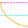
Shown in Figure 1 are results from an experimental setup where STD achieves superior accuracy as compared to STA in two distinct experiments (before and after distortion). The input signal to this virtual neuron was uniform white noise sampled at 1kHz distorted by a second order kernel. The stimulus drove a neuron which had a first order kernel and spiked when the convolved signal crossed a fixed threshold where each spike had an impact according to an exponential decay function describing an AHP. The STA kernel yields an error of 50%percent5050\% (cyan) as defined by |kdesklrn||kdes|subscript𝑘𝑑𝑒𝑠subscript𝑘𝑙𝑟𝑛subscript𝑘𝑑𝑒𝑠\frac{|k_{des}-k_{lrn}|}{|k_{des}|} where |||\cdot| is the L2subscript𝐿2L_{2} norm.

Adding signal distortion via a second order kernel creates a signal (1(a)) that results in STA having high frequency oscillation about the origin with an error of 119%percent119119\% (red) which when smoothed had an error of 98%percent9898\% (magenta). For comparison purposes, instead of randomly initializing, STD is using the scaled and smoothed STA result (magenta) as a starting place for gradient updates until convergence. This proceeds by randomly selecting one of the 100100100 input slices (1(a)) 10,0001000010,000 times and eventually yields an 8%percent88\% error (orange). To reiterate, STD achieved superior results while retraining on the same data and not over fitting! When trying to obtain a close approximation, to avoid compounding errors in complex analyses, it would be favorable to use STD.

Refer to caption
(a)
Refer to caption
(b)
Refer to caption
(c)
Figure 1: a, The input is distorted by passing it through a second order kernel modeled by a grid made of 20×20202020\times 20 third order cardinal B-splines. This produces a new signal that is used instead as input s=Kx(tτ1)x(tτ2)𝑑τ1𝑑τ2𝑠𝐾𝑥𝑡subscript𝜏1𝑥𝑡subscript𝜏2differential-dsubscript𝜏1differential-dsubscript𝜏2s=\int\int Kx(t-\tau_{1})x(t-\tau_{2})d\tau_{1}d\tau_{2}. The first and last 555 of 100100100 input slices of 200ms200𝑚𝑠200ms are shown sequentially. b, The distorted input leads to a high frequency STA kernel (red) which is then smoothed (magenta). STD proceeds from here by iterating through a chain of intermediary learning kernels (black) to approximate (orange) the desired (green). The undistorted input’s result before (blue) and after (cyan) smoothing show the effect the distortion has on STA. c, The error, as measured by |kdesklrn||kdes|subscript𝑘𝑑𝑒𝑠subscript𝑘𝑙𝑟𝑛subscript𝑘𝑑𝑒𝑠\frac{|k_{des}-k_{lrn}|}{|k_{des}|}, decreases to 8%percent88\% (orange) as the STD kernel approaches the desired. Smoothing and scaling the undistorted and distorted STA results improves them from 58%percent5858\% (blue) to 50%percent5050\% (cyan) and from 119%percent119119\% (red) to 98%percent9898\% (magenta).

Why STA requires Gaussian input

A graphical summary of how the LNP model operates is shown in Figure 2. The linear component is the first order Volterra kernel k𝑘k, the nonlinear component (N) is a function v𝑣v that maps the kernel response y=kxw𝑦𝑘subscript𝑥𝑤y=k*x_{w} to a firing rate z𝑧z, and an inhomogeneous Poisson (P) process generates spikes. At any point in time, the probability of firing is z=v(kxw)𝑧𝑣𝑘subscript𝑥𝑤z=v(k*x_{w}). The solution to the STA kernel can be expressed as k=ϕxx1ϕxy𝑘superscriptsubscriptitalic-ϕ𝑥𝑥1subscriptitalic-ϕ𝑥𝑦k=\phi_{xx}^{-1}\phi_{xy} where ϕxxsubscriptitalic-ϕ𝑥𝑥\phi_{xx} is the signal’s autocorrelation and ϕxysubscriptitalic-ϕ𝑥𝑦\phi_{xy} is the correlation of the signal with the potential. Instead of ϕxysubscriptitalic-ϕ𝑥𝑦\phi_{xy}, we can instead only observe a correlation with the spike rate ϕxzsubscriptitalic-ϕ𝑥𝑧\phi_{xz}. Bussgang[11] showed ϕxy=Cϕxzsubscriptitalic-ϕ𝑥𝑦𝐶subscriptitalic-ϕ𝑥𝑧\phi_{xy}=C\phi_{xz} the resulting kernel differs only by a scaling factor after the nonlinearity is applied, when the input is a Gaussian process.

Refer to caption
Figure 2: A signal is convolved with a linear kernel (L), passed through a nonlinearity (N) to achieve a spike rate, and then Poisson sampled (P) to produce spikes.

Generalized cumulative spike response model

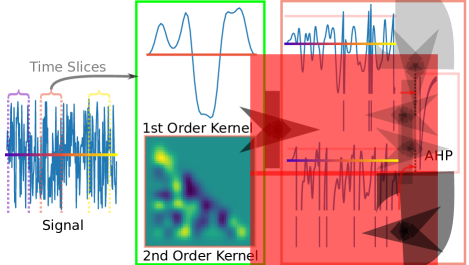
The cumulative spike response model (CSRM) [12] illustrated in Figure 3 can be generalized to include the full Volterra series of kernels (1). These kernels, approximated here by splines, represent the impact on the membrane potential by the stimuli’s higher order auto-correlates. Increasing n𝑛n allows for increased pattern detection capabilities. The AHP function η=Ae(tltk)/μ𝜂𝐴superscript𝑒subscript𝑡𝑙subscript𝑡𝑘𝜇\eta=-Ae^{(t_{l}-t_{k})/\mu} models the refractory period which is a region where spikes are highly unlikely to occur right after firing. In contrast to Poisson sampling, the AHP approach is deterministic and imposes a prior state dependency. A spike is generated when a threshold (Θ~~Θ\tilde{\Theta}) is exceeded by the signal convolved with kernel(s) minus past spikes’ AHPs. The n-order kernel Knsubscript𝐾𝑛K_{n} is a spline function composed of the n-ary Cartesian product of third order cardinal B-splines Bnsubscript𝐵𝑛B_{n}. The kernel is incrementally updated by the optimization process. At time t=tlO𝑡subscriptsuperscript𝑡𝑂𝑙t=t^{O}_{l} the kernel is Kl,n=iBi,l,nβi,l,nsubscript𝐾𝑙𝑛subscript𝑖subscript𝐵𝑖𝑙𝑛subscript𝛽𝑖𝑙𝑛K_{l,n}=\sum_{i}B_{i,l,n}\beta_{i,l,n}. The current and prior spike times are tlOsubscriptsuperscript𝑡𝑂𝑙t^{O}_{l} and tkOsubscriptsuperscript𝑡𝑂𝑘t^{O}_{k}. The AHP parameter μ𝜇\mu modifies the refractory time.

Θ~=n=1Kl,n(τ1τn;βi,l,n)inx(tlOτi)dτi+kη(tlOtkO;μ)~Θsuperscriptsubscript𝑛1subscript𝐾𝑙𝑛subscript𝜏1subscript𝜏𝑛subscript𝛽𝑖𝑙𝑛superscriptsubscriptproduct𝑖𝑛𝑥superscriptsubscript𝑡𝑙𝑂subscript𝜏𝑖𝑑subscript𝜏𝑖subscript𝑘𝜂superscriptsubscript𝑡𝑙𝑂superscriptsubscript𝑡𝑘𝑂𝜇\begin{split}\tilde{\Theta}=&\sum_{n=1}^{\infty}\int\ldots\int K_{l,n}(\tau_{1}\ldots\tau_{n};\beta_{i,l,n})\prod_{i}^{n}x(t_{l}^{O}-\tau_{i})d\tau_{i}+\sum_{k}\eta(t_{l}^{O}-t_{k}^{O};\mu)\end{split} (1)
Refer to caption
Figure 3: Slices of the uniformly random generated signal are serially passed through a kernel to produce a simulated electrical potential. When above threshold (pink) an AHP, with time constant μ𝜇\mu generally set to 1.2ms1.2𝑚𝑠1.2ms, is applied and a spike is produced which collectively (red box) inhibit future firing.

Theoretical overview of STD

Spike-triggered descent updates parameters based off of the distance between simulated and desired spike trains. To support using the distance (4) from [14] on the GCSRM, it is important to also generalize spike trains and show that they’re a subset of a vector space with an inner product ,\langle\cdot,\cdot\rangle. Considering augmented spike trains with countably infinite (={1,2,}12\mathbb{N}=\{1,2,...\}) spikes gives the framework the versatility to compare spike trains of any length. The augmentation turns spike trains into tuples of times and coefficients 𝒕={(ti,αi)}𝒕subscript𝑡𝑖subscript𝛼𝑖\bm{t}=\{(t_{i},\alpha_{i})\}. This forms a vector space and provides the foundation for creating an inner product (2) that induces a metric (Methods). Setting the αssuperscript𝛼𝑠\alpha^{\prime}s to 111 for finitely many spikes reduces to the usual space of spike trains within a bounded past. This is a subset of the generalization with the same metric and is squared to simplify the algebra (3).

𝒕𝑨,𝒕𝑩=i,j=1(αiA×αjB)tiA×tjB(tiA+tjB)2etiA+tjBτsuperscript𝒕𝑨superscript𝒕𝑩superscriptsubscript𝑖𝑗1superscriptsubscript𝛼𝑖𝐴superscriptsubscript𝛼𝑗𝐵superscriptsubscript𝑡𝑖𝐴superscriptsubscript𝑡𝑗𝐵superscriptsuperscriptsubscript𝑡𝑖𝐴superscriptsubscript𝑡𝑗𝐵2superscript𝑒superscriptsubscript𝑡𝑖𝐴superscriptsubscript𝑡𝑗𝐵𝜏\langle\bm{t^{A}},\bm{t^{B}}\rangle=\sum_{i,j=1}^{\infty}(\alpha_{i}^{A}\times\alpha_{j}^{B})\frac{t_{i}^{A}\times t_{j}^{B}}{(t_{i}^{A}+t_{j}^{B})^{2}}e^{-\frac{t_{i}^{A}+t_{j}^{B}}{\tau}} (2)
E=d2=𝒕𝑫𝒕𝑶,𝒕𝑫𝒕𝑶𝐸superscript𝑑2superscript𝒕𝑫superscript𝒕𝑶superscript𝒕𝑫superscript𝒕𝑶E=d^{2}=\langle\bm{t^{D}}-\bm{t^{O}},\bm{t^{D}}-\bm{t^{O}}\rangle (3)

Setting α𝛼\alpha values to 1 for N,M𝑁𝑀N,M spikes, and 0 otherwise, we get:

E(𝒕𝑫,𝒕𝑶)=i,j=1M,MtiD×tjD(tiD+tjD)2etiD+tjDτ+i,j=1N,NtiO×tjO(tiO+tjO)2etiO+tjOτ2i,j=1M,NtiD×tjO(tiD+tjO)2etiD+tjOτ𝐸superscript𝒕𝑫superscript𝒕𝑶superscriptsubscript𝑖𝑗1𝑀𝑀superscriptsubscript𝑡𝑖𝐷superscriptsubscript𝑡𝑗𝐷superscriptsuperscriptsubscript𝑡𝑖𝐷superscriptsubscript𝑡𝑗𝐷2superscript𝑒superscriptsubscript𝑡𝑖𝐷superscriptsubscript𝑡𝑗𝐷𝜏superscriptsubscript𝑖𝑗1𝑁𝑁superscriptsubscript𝑡𝑖𝑂superscriptsubscript𝑡𝑗𝑂superscriptsuperscriptsubscript𝑡𝑖𝑂superscriptsubscript𝑡𝑗𝑂2superscript𝑒superscriptsubscript𝑡𝑖𝑂superscriptsubscript𝑡𝑗𝑂𝜏2superscriptsubscript𝑖𝑗1𝑀𝑁superscriptsubscript𝑡𝑖𝐷superscriptsubscript𝑡𝑗𝑂superscriptsuperscriptsubscript𝑡𝑖𝐷superscriptsubscript𝑡𝑗𝑂2superscript𝑒superscriptsubscript𝑡𝑖𝐷superscriptsubscript𝑡𝑗𝑂𝜏\begin{split}E(\bm{t^{D}},\bm{t^{O}})=&\sum_{i,j=1}^{M,M}\frac{t_{i}^{D}\times t_{j}^{D}}{(t_{i}^{D}+t_{j}^{D})^{2}}e^{-\frac{t_{i}^{D}+t_{j}^{D}}{\tau}}\\ &+\sum_{i,j=1}^{N,N}\frac{t_{i}^{O}\times t_{j}^{O}}{(t_{i}^{O}+t_{j}^{O})^{2}}e^{-\frac{t_{i}^{O}+t_{j}^{O}}{\tau}}\\ &-2\sum_{i,j=1}^{M,N}\frac{t_{i}^{D}\times t_{j}^{O}}{(t_{i}^{D}+t_{j}^{O})^{2}}e^{-\frac{t_{i}^{D}+t_{j}^{O}}{\tau}}\end{split} (4)

A diagram of the generalized version of spikes is shown in Figure 4(a). It illustrates scalar multiplication (cyan) and vector addition (red). The vectors point positively into the past from the current time at zero. Multiplying the vector 𝒕𝑨superscript𝒕𝑨\bm{t^{A}} by 222 has the effect of doubling the coefficient for each time (cyan). When vectors 𝒕𝑨superscript𝒕𝑨\bm{t^{A}} and 𝒕𝑩superscript𝒕𝑩\bm{t^{B}} are added, equal times cause their coefficients to be added, else concatenated. Coefficients which sum to zero cause the spike to be deleted.

𝒕𝑨+𝒕𝑩superscript𝒕𝑨superscript𝒕𝑩\bm{t^{A}}+\bm{t^{B}}
2𝒕𝑨2superscript𝒕𝑨2\bm{t^{A}}
𝒕𝑨superscript𝒕𝑨\bm{t^{A}}
𝒕𝑩superscript𝒕𝑩\bm{t^{B}}
Refer to caption
Past
(a)
(Dt1βi,1Dt2βi,2Dt3βi,3Dt4βi,4=t4βi,40Dt2βi,1Dt3βi,2Dt4βi,3=Dt3βi,3t4t300Dt3βi,1Dt4βi,2=Dt3βi,2t4t3+Dt2βi,2t4t2000Dt4βi,1=Dt3βi,1t4t3+Dt2βi,1t4t2+Dt1βi,1t4t1)matrix𝐷subscript𝑡1subscript𝛽𝑖1𝐷subscript𝑡2subscript𝛽𝑖2𝐷subscript𝑡3subscript𝛽𝑖3𝐷subscript𝑡4subscript𝛽𝑖4subscript𝑡4subscript𝛽𝑖40𝐷subscript𝑡2subscript𝛽𝑖1𝐷subscript𝑡3subscript𝛽𝑖2𝐷subscript𝑡4subscript𝛽𝑖3𝐷subscript𝑡3subscript𝛽𝑖3subscript𝑡4subscript𝑡300𝐷subscript𝑡3subscript𝛽𝑖1𝐷subscript𝑡4subscript𝛽𝑖2𝐷subscript𝑡3subscript𝛽𝑖2subscript𝑡4subscript𝑡3𝐷subscript𝑡2subscript𝛽𝑖2subscript𝑡4subscript𝑡2000𝐷subscript𝑡4subscript𝛽𝑖1𝐷subscript𝑡3subscript𝛽𝑖1subscript𝑡4subscript𝑡3𝐷subscript𝑡2subscript𝛽𝑖1subscript𝑡4subscript𝑡2𝐷subscript𝑡1subscript𝛽𝑖1subscript𝑡4subscript𝑡1\displaystyle\begin{pmatrix}\begin{array}[]{cccl}{\color[rgb]{0,0,1}\definecolor[named]{pgfstrokecolor}{rgb}{0,0,1}\frac{Dt_{1}}{\partial\beta_{i,1}}}&{\color[rgb]{0,1,0}\definecolor[named]{pgfstrokecolor}{rgb}{0,1,0}\frac{Dt_{2}}{\partial\beta_{i,2}}}&{\color[rgb]{1,0,0}\definecolor[named]{pgfstrokecolor}{rgb}{1,0,0}\frac{Dt_{3}}{\partial\beta_{i,3}}}&{\color[rgb]{0,1,1}\definecolor[named]{pgfstrokecolor}{rgb}{0,1,1}\pgfsys@color@cmyk@stroke{1}{0}{0}{0}\pgfsys@color@cmyk@fill{1}{0}{0}{0}\frac{Dt_{4}}{\partial\beta_{i,4}}=\frac{\partial t_{4}}{\partial\beta_{i,4}}}\\ 0&{\color[rgb]{0,0,1}\definecolor[named]{pgfstrokecolor}{rgb}{0,0,1}\frac{Dt_{2}}{\partial\beta_{i,1}}}&{\color[rgb]{0,1,0}\definecolor[named]{pgfstrokecolor}{rgb}{0,1,0}\frac{Dt_{3}}{\partial\beta_{i,2}}}&{\color[rgb]{1,0,0}\definecolor[named]{pgfstrokecolor}{rgb}{1,0,0}\frac{Dt_{4}}{\partial\beta_{i,3}}=\frac{Dt_{3}}{\partial\beta_{i,3}}\frac{\partial t_{4}}{\partial t_{3}}}\\ 0&0&{\color[rgb]{0,0,1}\definecolor[named]{pgfstrokecolor}{rgb}{0,0,1}\frac{Dt_{3}}{\partial\beta_{i,1}}}&{\color[rgb]{0,1,0}\definecolor[named]{pgfstrokecolor}{rgb}{0,1,0}\frac{Dt_{4}}{\partial\beta_{i,2}}=\frac{Dt_{3}}{\partial\beta_{i,2}}\frac{\partial t_{4}}{\partial t_{3}}+\frac{Dt_{2}}{\partial\beta_{i,2}}\frac{\partial t_{4}}{\partial t_{2}}}\\ 0&0&0&{\color[rgb]{0,0,1}\definecolor[named]{pgfstrokecolor}{rgb}{0,0,1}\frac{Dt_{4}}{\partial\beta_{i,1}}=\frac{Dt_{3}}{\partial\beta_{i,1}}\frac{\partial t_{4}}{\partial t_{3}}+\frac{Dt_{2}}{\partial\beta_{i,1}}\frac{\partial t_{4}}{\partial t_{2}}+\frac{Dt_{1}}{\partial\beta_{i,1}}\frac{\partial t_{4}}{\partial t_{1}}}\end{array}\end{pmatrix}
(b)
Figure 4: a, Two example spike trains 𝒕𝑨superscript𝒕𝑨\bm{t^{A}} (blue) and 𝒕𝑩superscript𝒕𝑩\bm{t^{B}} (green) under scalar multiplication 2𝒕𝑨2superscript𝒕𝑨2\bm{t^{A}} (cyan) and vector addition 𝒕𝑨+𝒕𝑩superscript𝒕𝑨superscript𝒕𝑩\bm{t^{A}}+\bm{t^{B}} (red). b, Example vectorization/memoization [15] for calculating the total derivatives of time changes with respect to changes in β𝛽\beta (8) for spline i𝑖i at each prior spike.

The GCSRM (1) describes when the threshold is equal to the sum of the convolution(s) minus past AHP effects. Perturbing its parameters, performing a first order Taylor approximation, and setting the perturbed and unperturbed expressions equal allows for the creation of partial derivatives with respect to the parameters β𝛽\beta (5), μ𝜇\mu (6), and tksubscript𝑡𝑘t_{k} (7) (Methods). These express how spike times change with respect to a change in spline coefficient, time constant, and prior spike time. These partial derivatives are used to calculate the total derivatives (8), an example for 444 spikes is shown in 4(b). The matrix for μ𝜇\mu is similar except that μ𝜇\mu only effects future spikes meaning tlμl=0subscript𝑡𝑙subscript𝜇𝑙0\frac{\partial t_{l}}{\partial\mu_{l}}=0. The total derivative for a spike time with respect to a parameter at a prior time is the sum of that parameter’s total effect on each of the more recent prior spikes each multiplied by the relevant time partial to tie it to the current time.

tlOβi,l=Bi(τ)x(tlOτ)𝑑τ0|K|K(τ;βi,l)xt|tlOτdτ+ηt|tlOtkOsuperscriptsubscript𝑡𝑙𝑂subscript𝛽𝑖𝑙subscript𝐵𝑖𝜏𝑥superscriptsubscript𝑡𝑙𝑂𝜏differential-d𝜏evaluated-atsuperscriptsubscript0𝐾𝐾𝜏subscript𝛽𝑖𝑙𝑥𝑡superscriptsubscript𝑡𝑙𝑂𝜏𝑑𝜏evaluated-at𝜂𝑡superscriptsubscript𝑡𝑙𝑂superscriptsubscript𝑡𝑘𝑂\frac{\partial t_{l}^{O}}{\partial\beta_{i,l}}=\frac{-\int B_{i}(\tau)x(t_{l}^{O}-\tau)d\tau}{\int_{0}^{|K|}K(\tau;\beta_{i,l})\frac{\partial x}{\partial t}\Big{|}_{t_{l}^{O}-\tau}d\tau+\sum\frac{\partial\eta}{\partial t}\Big{|}_{t_{l}^{O}-t_{k}^{O}}} (5)
tlOμl=ημ|tlOtkO0|K|K(τ;βi,l)xt|tlOτdτ+ηt|tlOtkOsuperscriptsubscript𝑡𝑙𝑂subscript𝜇𝑙evaluated-at𝜂𝜇superscriptsubscript𝑡𝑙𝑂superscriptsubscript𝑡𝑘𝑂evaluated-atsuperscriptsubscript0𝐾𝐾𝜏subscript𝛽𝑖𝑙𝑥𝑡superscriptsubscript𝑡𝑙𝑂𝜏𝑑𝜏evaluated-at𝜂𝑡superscriptsubscript𝑡𝑙𝑂superscriptsubscript𝑡𝑘𝑂\frac{\partial t_{l}^{O}}{\partial\mu_{l}}=\frac{-\frac{\partial\eta}{\partial\mu}\Big{|}_{t_{l}^{O}-t_{k}^{O}}}{\int_{0}^{|K|}K(\tau;\beta_{i,l})\frac{\partial x}{\partial t}\Big{|}_{t_{l}^{O}-\tau}d\tau+\sum\frac{\partial\eta}{\partial t}\Big{|}_{t_{l}^{O}-t_{k}^{O}}} (6)
tlOtkO=ηt|tlOtkO0|K|K(τ;βi,l)xt|tlOτdτ+ηt|tlOtkOsuperscriptsubscript𝑡𝑙𝑂superscriptsubscript𝑡𝑘𝑂evaluated-at𝜂𝑡superscriptsubscript𝑡𝑙𝑂superscriptsubscript𝑡𝑘𝑂evaluated-atsuperscriptsubscript0𝐾𝐾𝜏subscript𝛽𝑖𝑙𝑥𝑡superscriptsubscript𝑡𝑙𝑂𝜏𝑑𝜏evaluated-at𝜂𝑡superscriptsubscript𝑡𝑙𝑂superscriptsubscript𝑡𝑘𝑂\frac{\partial t_{l}^{O}}{\partial t_{k}^{O}}=\frac{\frac{\partial\eta}{\partial t}\Big{|}_{t_{l}^{O}-t_{k}^{O}}}{\int_{0}^{|K|}K(\tau;\beta_{i,l})\frac{\partial x}{\partial t}\Big{|}_{t_{l}^{O}-\tau}d\tau+\sum\frac{\partial\eta}{\partial t}\Big{|}_{t_{l}^{O}-t_{k}^{O}}} (7)
Dtk+1Oβi,l=tj>tlkDtjOβi,ltk+1OtjO𝐷superscriptsubscript𝑡𝑘1𝑂subscript𝛽𝑖𝑙superscriptsubscriptsubscript𝑡𝑗subscript𝑡𝑙𝑘𝐷superscriptsubscript𝑡𝑗𝑂subscript𝛽𝑖𝑙superscriptsubscript𝑡𝑘1𝑂superscriptsubscript𝑡𝑗𝑂\frac{Dt_{k+1}^{O}}{\partial\beta_{i,l}}=\sum_{t_{j}>t_{l}}^{k}\frac{Dt_{j}^{O}}{\partial\beta_{i,l}}\frac{\partial t_{k+1}^{O}}{\partial t_{j}^{O}} (8)

The total derivative expressions for each of the spikes with respect to a parameter are then connected via another chain rule to the squared distance E. This is performed by summing over the multiple of EtkO𝐸superscriptsubscript𝑡𝑘𝑂\frac{\partial E}{\partial t_{k}^{O}} along a (colored) diagonal in 4(b). The sum of all of these changes in E with respect to that parameter across all time steps is the gradient. The equations (9) and (10) are the gradient updates used to minimize the spike train distance with respect to the spline parameters β𝛽\beta and AHP time constant μ𝜇\mu. Using these gradients, small steps (with size α𝛼\alpha) are taken in accordance with sgd methods such as momentum [16] and katyusha [17]. The updates are best triggered soon after spikes since E exponentially decays as spikes are pushed further into the past.

βi=βiαβkFlEβi,lsubscript𝛽𝑖subscript𝛽𝑖subscript𝛼𝛽subscript𝑘subscript𝐹𝑙𝐸subscript𝛽𝑖𝑙\beta_{i}=\beta_{i}-\alpha_{\beta}\sum_{k\in F_{l}}\frac{\partial E}{\partial\beta_{i,l}} (9)
μ=μαμkFlEμk𝜇𝜇subscript𝛼𝜇subscript𝑘subscript𝐹𝑙𝐸subscript𝜇𝑘\mu=\mu-\alpha_{\mu}\sum_{k\in F_{l}}\frac{\partial E}{\partial\mu_{k}} (10)

Convergence of β𝛽\beta and μ𝜇\mu

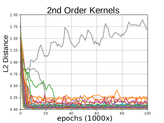
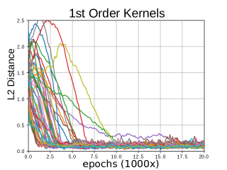
Convergence of first and second order kernels on simulated data are shown in Figure 5. While holding μ𝜇\mu fixed, the convergence for 50 trials of 1st (5(a)) and 2nd (5(b)) order kernels are demonstrated. An error, or L2subscript𝐿2L_{2} distance, of zero means the learning and desired kernels are equal. A variety of SGD methods were used: vanilla was too slow, katyusha was too unstable, and momentum was fast and relatively robust.

One simulation, seen in (5(b)), does not converge. These cases can arise for a variety of reasons and is often the result of hyperparameters: momentum, learning rate, cap, AHP threshold, and number of epochs. Lower learning rates and momentum converge more stably but require more iterations. For 2nd order kernels, a mask is applied to keep it lower triangular. This was used as a means of preventing diagonally symmetric terms from conflicting. The cap, a crucial parameter due to the highly nonlinear nature of the problem, is an upper bound on the L2subscript𝐿2L_{2} norm of the gradient step preventing unnecessarily large updates which lead to divergence.
Refer to caption
(a)
Refer to caption
(b)
Figure 5: a,b, Convergence for 505050 trials of 1st order kernels composed of 101010 splines and 2nd order kernels composed of a grid of 8×8888\times 8 splines. Each epoch represents an update and consists of a signal of 400400400 time units set as 1ms1𝑚𝑠1ms meant to be consistent with a statically set AHP time constant μ=1.2ms𝜇1.2𝑚𝑠\mu=1.2ms.

When the desired kernel is shorter than the learning kernel, the extra values become zero as would be expected. Convergence was best for these third order overlapping cardinal B-splines with 121212 abstract time units of nonzero support. Most tests were performed on 101010 splines. More splines took more training time and this was compounded by increasing the kernel’s order. The computational and space requirements of higher order kernels restrict consideration to fewer parameters.

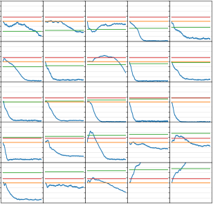
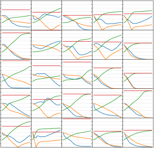
In Figure 6(a), the learning μ𝜇\mu (green) is set incorrectly from the desired μ𝜇\mu (red) and scanned for its effect on the convergence of the β𝛽\beta parameters. There is a larger region of stability below the desired μ𝜇\mu. The μ𝜇\mu (orange) and β𝛽\beta (blue) errors are normalized with respect to their initial distance from the desired. Demonstrated in 6(b), μ𝜇\mu and β𝛽\beta are being learned in tandem. Once the learning μ𝜇\mu grows larger than the desired, the simulations begin to diverge. This is because μ𝜇\mu’s effect is exponential and β𝛽\beta’s splines are linear. They cannot compensate for this error and this causes a feedback loop. Seeing as there was a large range of stability it is something that can easily be scanned. We also tried using a spline representation for the AHP, but getting the parameters to match required spikes to overlap with the spline. Some splines, particularly immediate after a firing, were the least likely to occur but also had the greatest impact. Other basis functions might be an option.
Refer to caption
(a)
Refer to caption
(b)
Figure 6: a, μ𝜇\mu (green) is scanned from 0.500.500.50 (top left) to 1.71.71.7 (bottom right) in steps of 0.050.050.05. For a desired μ=1.2𝜇1.2\mu=1.2 (red) a range for accurate convergence for β𝛽\beta (blue) corresponds to [0.65,1.35]0.651.35[0.65,1.35] or alternatively [54%,113%]percent54percent113[54\%,113\%] of the desired. b, Convergences are shown for μ𝜇\mu (orange) and β𝛽\beta (blue) being simultaneously learned and plotted as ratios from their original L2subscript𝐿2L_{2} distance.

Sensitivity to Noise: shifting addition and deletion of spikes

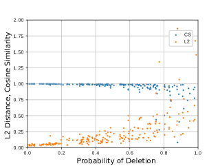
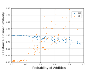
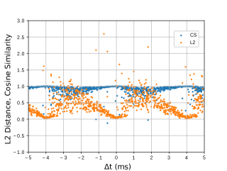
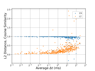
After giving STA difficulty with a complex AHP scenario, it was important to similarly challenge the capability of STD by from learning LNP spikes. This exploration was initiated by analyzing the effect on convergence by the shifting, adding, or deleting of spikes. Upon perturbing the spike times by some fixed amount (dt𝑑𝑡dt) it quickly became apparent that more granularity was needed in the AHP spike generation process itself. This lead to calculating a more precise intersection of the potential with the threshold and was achieved by linear interpolation. Figure 7 demonstrates the effects of adding noise to the CSRM system and the effect it has on convergence and cosine similarity defined by abab𝑎𝑏norm𝑎norm𝑏\frac{a\cdot b}{||a||\;||b||} which is chosen for its invariance to scaling.

Moving far away from dt=0𝑑𝑡0dt=0 resulted in divergence and indicated that the learning kernel needed flexibility. Padding both the learning and desired kernels with splines having β=0𝛽0\beta=0 allowed the learning kernel to appropriately shift (7(a)). Removing spikes (7(c)) randomly with some probability, normalized with respect to the number of spikes, had minimal effect on convergence until the deletion chance was 50%percent50~{}50\%. Real neurons are highly connected and auxiliary processing could cause additional seemingly random spikes. Adding spikes to any location (7(d)) shows that learning is comparatively more sensitive to addition.
Refer to caption
(a)
Refer to caption
(b)
Refer to caption
(c)
Refer to caption
(d)
Figure 7: a, Shifting spikes uniformly by a set amount resulted in a cyclic pattern as the 101010 splines snapped into alignment with adjacent splines. b, Randomly perturbing each desired spike separately about a normal distribution. c, d, Picking a homogeneous Possion rate for deleting (or adding) spikes reveals that as many as half (or a fifth) of the spikes could be deleted (or added) while still extracting a kernel with a low L2subscript𝐿2L_{2} distance.
Refer to caption
(a)
Refer to caption
(b)
Refer to caption
(c)
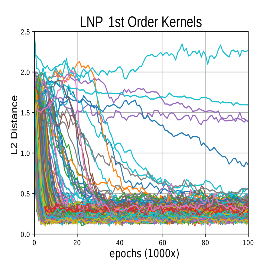
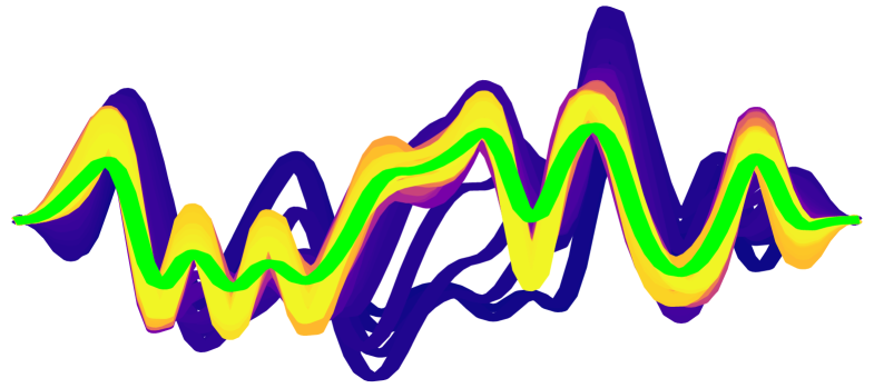
Figure 8: a, Convergence for 500500500 STD trials on a 444-binned LNP process learning 202020 splines of 80ms80𝑚𝑠80ms over 100,000100000100,000 epochs of length 400ms400𝑚𝑠400ms. b, Thirteenth worst convergence peaking at an L2subscript𝐿2L_{2} distance of 178%percent178178\% and ending at 42.3%percent42.342.3\%. c, Intermediary learning kernels vs the desired (lime).

STD’s success on spikes generated via an LNP process is explored in Figure 8. For the LNP model, a high exponential coefficient in the nonlinearity (a sigmoid) resulted in a firing rate which was mostly either 00 or 111. This made it crucial to center it around the threshold value. This resulted in too many spikes above threshold and none below. To obtain a corresponding amount of spikes in both the LNP and AHP models a mixture of modifications can be made: reducing μ𝜇\mu the AHP time constant, reducing the peak probability of spiking, and constraining the LNP time domain. The peak probability was set at 50%percent5050\% and the LNP spike time domain was binned down sampling by a factor of 444. Among the 500500500 cases, the average learning kernel had a 20%percent2020\% lower error.

Kernel for Locusta migratoria tympanal nerve

Sensory neurons which, when given the same stimuli, reliably produce similar spike trains are good candidates to test STD. One such possibility is the tympanal nerve’s auditory receptor axons in the Locusta migratoria grasshopper whose action potentials, recorded intracellularly, can have a 0.15ms0.15𝑚𝑠0.15ms[18] inter trial jitter. This dataset, collected by Ariel Rokem[19] [20] at the lab of Andreas Herz, was graciously shared through the CRCNS program (http://crcns.org) [1]. The stimuli consisted of a carrier wave perturbed by random amplitude modulations and a cutoff frequency of up to 800Hz800𝐻𝑧800Hz. We used a particular subset of this dataset to demonstrate kernel extraction.

Refer to caption   Refer to caption   Refer to caption   Refer to caption   


(a)


(b)
Figure 9: a, The Locusta migratoria spike data (blue and orange dots) collected by A. Rokem in cell “./crcns-ia1/Data1/03-04-23-ad/” corresponding to the “gauss_st6_co200.dat” stimuli with a cutoff frequency of 200Hz200𝐻𝑧200Hz. The recording is sliced up with milliseconds on the y axis and seconds on the x for a total of 101010 seconds. Each spike train consists of approximately 100010001000 spikes. The goal was to train an STD kernel that could reconstruct (green dashes) the desired (blue dashes) spike train. There are 555 other recordings (orange dashes) for this stimuli and cell. The final kernel’s simulated spike train closely approximates the desired. The green line represents error between the learning and desired spike trains from a preceding window of 100ms100𝑚𝑠100ms and is clipped to a range from 00 to 666. Similarly, the blue and red lines represent the minimum and maximum error between any pair of recorded spike trains. b, Zoomed sections of the reconstruction were randomly chosen. Notice that the learning error is often between the minimum and maximum errors between recordings. Additionally, a simulated spike will sometimes align with the other recordings even when the desired does not. These are indications that the kernel accurately represents underlying model.

Repeated updates lead to a kernel which attempts to reconstruct the provided spike train. When running a simulation with a known desired neuron the absolute distance between kernels can be measured. In absence of a known answer, and in lieu of a universally accepted metric, we revert to demonstrating the effectiveness by showcasing the simulated spike train reconstruction for a particular kernel. Figure 9 demonstrates this using a (stimuli, spike train) pair as input. The stimuli we used had a cutoff frequency of 200Hz200𝐻𝑧200Hz. The reconstruction (green dashes) was learned from (blue dashes) one of the 666 recorded spike trains for a particular cell (“./crcns-ia1/Data1/03-04-23-ad/”). The reconstruction occasionally fires where the desired does not but the other (orange dashes) recordings do. This is an indication that the underlying model is being accurately represented.

Refer to caption
Figure 10: The raw STA kernel (blue) spanning 100010001000 time units of 0.05ms0.05𝑚𝑠0.05ms was smoothed (orange) and compared with the STD result (green). The smoothed STA kernel was the result of of convolving 555 times against a box spline spanning 1ms1𝑚𝑠1ms.

Given that the data set was recorded at 0.05ms0.05𝑚𝑠0.05ms and borrowing inspiration from Nemenman’s work[21], showing that a blowfly’s H1 neuron represents information with sub-millisecond precision even for slow stimuli, finer time resolution STD kernels were explored. The best observed reconstruction was for an STD kernel (green) composed of 505050 splines and four 0.25ms0.25𝑚𝑠0.25ms units per knot interval shown in Figure 10 along with raw (blue) and smoothed (orange) STA kernels. The STA results were omitted from Figure 9 due to a large variety of low quality reconstructions. It was trained with all 666 recorded spike trains, different sized kernels, various levels of smoothing, and multiple spike generation methods (LNP, CSRM). STD is a better technique for learning kernels that have the ability to reconstruct spike trains.

Discussion

STD, unlike STA, can learn higher order kernels and generate spike trains to verify the accuracy of its approximation. STA is restricted to linear kernels and doesn’t provide a nonlinearity for reconstruction. STD provides a better kernel approximation than STA in our simulated examples. Robustness to a variety of noise and a cross model comparison indicate its potential to be widely applicable. The simulated reconstructions of the Locusta migratoria spike trains are closely aligned which indicates that STD can extract the kernel from many different neural systems.

The primary concern is that model mismatch might make convergence impossible. Unfortunately, this could be confused with incorrect hyperparameters such as the cap, AHP value, threshold, learning rate, momentum, and epochs. Convergence can be measured in terms of parameter stabilization, the predictive ability of the simulation, and with the spike train distance. Multiple simulations can be run from different initializations, but convergence to the same parameter set does not imply a correct solution. This was first seen when trying to learn LNP spike trains where settings stably converged to an incorrect parameter set. This was due to an incompatible model mismatch and was fixed by down sampling.

Slowly changing kernels could be learned from slices of the signal and interpolating the intermediary results. The implementation of the second order kernel operations are similar enough to first order such that core pieces of code can be left untouched for further generalization. The lowest hanging fruit for this technique would be to apply it to other existing datasets. Expanding the code to work for video inputs is another avenue for future research.

Acknowledgments

Anik Chattopadhyay and Daniel Crews for their assistance with theory and troubleshooting, Kyle Altendorf (@altendky) and Aleksi Torhamo (@Alexer) via #python on IRC in freenode for help with profiling and vectorizing calculations. And thanks to Ariel Rokem for sharing the Locusta migratoria dataset and CRCNS for hosting it. This work was partially funded by AFOSR grant #FA9550-16-1-0135.

Materials and Methods

Spike Triggered Average as an optimization

Ignoring the nonlinearity due to the proportionality via Bussgang’s equation 20 [11] leads to an optimization problem. In the discrete time framework, each successive |k|𝑘|k| sized slice of a signal x𝑥x forms a row of a matrix X𝑋X. The convolution of the kernel with a corresponding section of the signal kxw𝑘subscript𝑥𝑤k*x_{w} becomes Xk𝑋𝑘Xk. The resulting simulated electrical potential from the convolution is labeled y𝑦y. The optimization problem can then be phrased min(Xky2)𝑚𝑖𝑛superscriptnorm𝑋𝑘𝑦2min(||Xk-y||^{2}). To solve for k𝑘k let a partial derivative operator D=kT𝐷superscript𝑘𝑇D=\frac{\partial}{\partial k^{T}} operate on Xky2=(Xky)T(Xky)=kTXTXkkTXTyyTXk+yTysuperscriptnorm𝑋𝑘𝑦2superscript𝑋𝑘𝑦𝑇𝑋𝑘𝑦superscript𝑘𝑇superscript𝑋𝑇𝑋𝑘superscript𝑘𝑇superscript𝑋𝑇𝑦superscript𝑦𝑇𝑋𝑘superscript𝑦𝑇𝑦||Xk-y||^{2}=(Xk-y)^{T}(Xk-y)=k^{T}X^{T}Xk-k^{T}X^{T}y-y^{T}Xk+y^{T}y so that DXky2=2XTXk2XTY=0𝐷superscriptnorm𝑋𝑘𝑦22superscript𝑋𝑇𝑋𝑘2superscript𝑋𝑇𝑌0D||Xk-y||^{2}=2X^{T}Xk-2X^{T}Y=0 and k=(XTX)1XTY𝑘superscriptsuperscript𝑋𝑇𝑋1superscript𝑋𝑇𝑌k=(X^{T}X)^{-1}X^{T}Y. This formulation is termed whitened STA.

Third order cardinal B-Splines

Central to STD is the ability to tune parametrized kernels to decrease the spike distance. These kernels are spline functions composed of third order Cardinal B-splines. This causes them to be everywhere differentiable with respect to time. Starting with the recurrence relation in equation (15) (page 90 [22], page 143 [23]), the B-Spline coefficients from [24] are shown in equation (11). The number of steps within each knot sequence was set to 444 time units. The kernel is constructed by summing the multiple of all splines with their corresponding scaling parameters (12). The n𝑛n order kernels Knsubscript𝐾𝑛K_{n} are formed by B-splines Bi,nsubscript𝐵𝑖𝑛B_{i,n} which are the n-ary Cartesian product of one dimensional splines. This is a deviation from the standard notation where n𝑛n refers instead to the order of the spline which was always 333 in our experiments.

B0,3={x[0,1)12x2x[1,2)x2+3x32x[2,3)12x23x+92x[0,3)0subscript𝐵03cases𝑥0112superscript𝑥2𝑥12superscript𝑥23𝑥32𝑥2312superscript𝑥23𝑥92𝑥030B_{0,3}=\begin{cases}x\in[0,1)&\frac{1}{2}x^{2}\\ x\in[1,2)&-x^{2}+3x-\frac{3}{2}\\ x\in[2,3)&\frac{1}{2}x^{2}-3x+\frac{9}{2}\\ x\notin[0,3)&0\end{cases} (11)
Kn=i=0Bi,nβisubscript𝐾𝑛subscript𝑖0subscript𝐵𝑖𝑛subscript𝛽𝑖K_{n}=\sum_{i=0}B_{i,n}\beta_{i} (12)

Verifying the coefficients from [24] using the recursion formulas (13) and (14) from [22] combine into (15). The final representation, displayed similarly to [25], represents what the value of the spline is for each section of its support. This is also commonly displayed as a matrix where elements represent polynomial coefficients [24]. Setting k=3𝑘3k=3 leads to it being a third order and the knot sequence increasing as counting numbers makes these third order cardinal splines. Successive support regions increment j𝑗j by 111 causing an overlap of the nonzero region with the adjacent splines. Adding additional evaluations within each knot range have the effect of smoothing the spline at the cost of taking up more time units.

Bj,k:=wj,kBj,k1+(1wj+1,k)Bj+1,k1assignsubscript𝐵𝑗𝑘subscript𝑤𝑗𝑘subscript𝐵𝑗𝑘11subscript𝑤𝑗1𝑘subscript𝐵𝑗1𝑘1B_{j,k}:=w_{j,k}B_{j,k-1}+(1-w_{j+1,k})B_{j+1,k-1} (13)
wj,k(x):=xtjtj+k1tjassignsubscript𝑤𝑗𝑘𝑥𝑥subscript𝑡𝑗subscript𝑡𝑗𝑘1subscript𝑡𝑗w_{j,k}(x):=\frac{x-t_{j}}{t_{j+k-1}-t_{j}} (14)
Bj,k:=xtjtj+k1tjBj,k1+tj+kxtj+ktj+1Bj+1,k1assignsubscript𝐵𝑗𝑘𝑥subscript𝑡𝑗subscript𝑡𝑗𝑘1subscript𝑡𝑗subscript𝐵𝑗𝑘1subscript𝑡𝑗𝑘𝑥subscript𝑡𝑗𝑘subscript𝑡𝑗1subscript𝐵𝑗1𝑘1B_{j,k}:=\frac{x-t_{j}}{t_{j+k-1}-t_{j}}B_{j,k-1}+\frac{t_{j+k}-x}{t_{j+k}-t_{j+1}}B_{j+1,k-1} (15)
k=3𝑘3k=3
Bj,3:=xtjtj+2tjBj,2+tj+3xtj+3tj+1Bj+1,2assignsubscript𝐵𝑗3𝑥subscript𝑡𝑗subscript𝑡𝑗2subscript𝑡𝑗subscript𝐵𝑗2subscript𝑡𝑗3𝑥subscript𝑡𝑗3subscript𝑡𝑗1subscript𝐵𝑗12B_{j,3}:=\frac{x-t_{j}}{t_{j+2}-t_{j}}B_{j,2}+\frac{t_{j+3}-x}{t_{j+3}-t_{j+1}}B_{j+1,2} (16)
Bj,2:=xtjtj+1tjBj,1+tj+2xtj+2tj+1Bj+1,1assignsubscript𝐵𝑗2𝑥subscript𝑡𝑗subscript𝑡𝑗1subscript𝑡𝑗subscript𝐵𝑗1subscript𝑡𝑗2𝑥subscript𝑡𝑗2subscript𝑡𝑗1subscript𝐵𝑗11B_{j,2}:=\frac{x-t_{j}}{t_{j+1}-t_{j}}B_{j,1}+\frac{t_{j+2}-x}{t_{j+2}-t_{j+1}}B_{j+1,1} (17)
Bj,1:={x[tj,tj+1)1x[tj,tj+1)0assignsubscript𝐵𝑗1cases𝑥subscript𝑡𝑗subscript𝑡𝑗11𝑥subscript𝑡𝑗subscript𝑡𝑗10B_{j,1}:=\begin{cases}x\in[t_{j},t_{j+1})&1\\ x\notin[t_{j},t_{j+1})&0\end{cases} (18)
j=0t=[0,1,2,3]formulae-sequence𝑗0𝑡0123j=0\hskip 28.45274ptt=[0,1,2,3] (19)
B0,3:=xt0t2t0B0,2+t3xt3t1B1,2=x020B0,2+3x31B1,2=x2B0,2+3x2B1,2assignsubscript𝐵03𝑥subscript𝑡0subscript𝑡2subscript𝑡0subscript𝐵02subscript𝑡3𝑥subscript𝑡3subscript𝑡1subscript𝐵12𝑥020subscript𝐵023𝑥31subscript𝐵12𝑥2subscript𝐵023𝑥2subscript𝐵12\begin{split}B_{0,3}:=\frac{x-t_{0}}{t_{2}-t_{0}}B_{0,2}&+\frac{t_{3}-x}{t_{3}-t_{1}}B_{1,2}\\ =\frac{x-0}{2-0}B_{0,2}&+\frac{3-x}{3-1}B_{1,2}\\ =\frac{x}{2}B_{0,2}&+\frac{3-x}{2}B_{1,2}\end{split} (20)
B0,2:=x010B0,1+2x21B1,1=x1B0,1+2x1B1,1assignsubscript𝐵02𝑥010subscript𝐵012𝑥21subscript𝐵11𝑥1subscript𝐵012𝑥1subscript𝐵11\begin{split}B_{0,2}:=\frac{x-0}{1-0}B_{0,1}+&\frac{2-x}{2-1}B_{1,1}\\ =\frac{x}{1}B_{0,1}+&\frac{2-x}{1}B_{1,1}\end{split} (21)
B0,1:={x[0,1)1x[0,1)0assignsubscript𝐵01cases𝑥011𝑥010B_{0,1}:=\begin{cases}x\in[0,1)&1\\ x\notin[0,1)&0\end{cases} (22)
B1,2:=x121B1,1+3x32B2,1=x11B1,0+3x1B2,0assignsubscript𝐵12𝑥121subscript𝐵113𝑥32subscript𝐵21𝑥11subscript𝐵103𝑥1subscript𝐵20\begin{split}B_{1,2}:=&\frac{x-1}{2-1}B_{1,1}+\frac{3-x}{3-2}B_{2,1}\\ =&\frac{x-1}{1}B_{1,0}+\frac{3-x}{1}B_{2,0}\end{split} (23)
B0,3=x2(x1B0,1+2x1B1,1)+3x2(x11B1,1+3x1B2,1)subscript𝐵03𝑥2𝑥1subscript𝐵012𝑥1subscript𝐵113𝑥2𝑥11subscript𝐵113𝑥1subscript𝐵21\begin{split}B_{0,3}=&\frac{x}{2}(\frac{x}{1}B_{0,1}+\frac{2-x}{1}B_{1,1})\\ &+\frac{3-x}{2}(\frac{x-1}{1}B_{1,1}+\frac{3-x}{1}B_{2,1})\end{split} (24)
B0,3={x[0,1)x2x1x[1,2)x22x1+3x2x11x[2,3)3x23x1x[0,3)0subscript𝐵03cases𝑥01𝑥2𝑥1𝑥12𝑥22𝑥13𝑥2𝑥11𝑥233𝑥23𝑥1𝑥030B_{0,3}=\begin{cases}x\in[0,1)&\frac{x}{2}\frac{x}{1}\\ x\in[1,2)&\frac{x}{2}\frac{2-x}{1}+\frac{3-x}{2}\frac{x-1}{1}\\ x\in[2,3)&\frac{3-x}{2}\frac{3-x}{1}\\ x\notin[0,3)&0\end{cases} (25)
B0,3={x[0,1)12x2x[1,2)x2+3x32x[2,3)12x23x+92x[0,3)0subscript𝐵03cases𝑥0112superscript𝑥2𝑥12superscript𝑥23𝑥32𝑥2312superscript𝑥23𝑥92𝑥030B_{0,3}=\begin{cases}x\in[0,1)&\frac{1}{2}x^{2}\\ x\in[1,2)&-x^{2}+3x-\frac{3}{2}\\ x\in[2,3)&\frac{1}{2}x^{2}-3x+\frac{9}{2}\\ x\notin[0,3)&0\end{cases} (26)

Spike trains as a vector space

Spike trains can be generalized and transformed into a vector space. This is achieved by augmenting them to include coefficients for each spike time along with defining appropriate addition and multiplication operations such that vector space properties are satisfied. Sequence spaces are similar constructions that have a simpler addition operator due to their natural ordering. These augmented spike trains are sequences of 2-tuples which have 5 primary properties: (27), (28), (29), (30), and (31). The times are exclusively in the past (28) and are ordered so that they are strictly increasing (29). The coefficients can be any non zero value in \mathbb{R} (27). These sequences can be finite or countably infinite (30) and are confined to a subspace where the sum of the coefficients converges absolutely (31).

αi{0}subscript𝛼𝑖0\alpha_{i}\in\mathbb{R}-\{0\} (27)
ti>0subscript𝑡𝑖subscriptabsent0t_{i}\in\mathbb{R}_{>0} (28)
ti<tji<jsubscript𝑡𝑖subscript𝑡𝑗for-all𝑖𝑗t_{i}<t_{j}\forall i<j (29)
i,j𝑖𝑗i,j\in\mathbb{N} (30)
i=0|αi|<superscriptsubscript𝑖0subscript𝛼𝑖\sum_{i=0}^{\infty}|\alpha_{i}|<\infty (31)

Definition: Let V𝑉V be the space of finite or countably infinite sequences of time ordered 2-tuples 𝒕={(ti,αi)}V𝒕subscript𝑡𝑖subscript𝛼𝑖𝑉\bm{t}=\{(t_{i},\alpha_{i})\}\in V such that (27), (28), (29), (30), and (31) hold.

Adding these augmented spike trains results in a new sequence that consists of adding temporally corresponding coefficients and otherwise concatenating. Defining two intermediary operators (32) and (33) allows for a simpler addition definition for these sequences (34). The spike train vectors 𝒕𝑨,𝒕𝑩Vsuperscript𝒕𝑨superscript𝒕𝑩𝑉\bm{t^{A}},\bm{t^{B}}\in V with times tiA,tjBsuperscriptsubscript𝑡𝑖𝐴superscriptsubscript𝑡𝑗𝐵t_{i}^{A},t_{j}^{B} and coefficients αiA,αjBsuperscriptsubscript𝛼𝑖𝐴superscriptsubscript𝛼𝑗𝐵\alpha_{i}^{A},\alpha_{j}^{B} correspond to different spike trains A,B𝐴𝐵A,B. Selecting tuples where the time only occurs in the first spike train can be expressed by a modified version (32) of the set difference operator (AB𝐴𝐵A\setminus B). The set theory intersection operator \cap can be redefined (33) to select where the same time exists in both while adding coefficients and deleting tuples with zero coefficients. The unioned sets in (34) are always disjoint so \cup does not need to be modified.

𝒕𝑨𝒕𝑩={(tiA,αiA):(tiA,αiA)𝒕𝑨 and (tjB,)𝒕𝑩 and tiA=tjB}superscript𝒕𝑨superscript𝒕𝑩conditional-setsuperscriptsubscript𝑡𝑖𝐴superscriptsubscript𝛼𝑖𝐴superscriptsubscript𝑡𝑖𝐴superscriptsubscript𝛼𝑖𝐴superscript𝒕𝑨 and superscriptsubscript𝑡𝑗𝐵superscript𝒕𝑩 and superscriptsubscript𝑡𝑖𝐴superscriptsubscript𝑡𝑗𝐵\bm{t^{A}}\setminus\bm{t^{B}}=\{(t_{i}^{A},\alpha_{i}^{A}):(t_{i}^{A},\alpha_{i}^{A})\in\bm{t^{A}}\text{ and }(t_{j}^{B},\cdot)\notin\bm{t^{B}}\text{ and }t_{i}^{A}=t_{j}^{B}\} (32)
𝒕𝑨𝒕𝑩={(tiA,αiA+αjB):(tiA,αiA)𝒕𝑨 and (tjB,αjB)𝒕𝑩,tiA=tjB and αiA+αjB0}superscript𝒕𝑨superscript𝒕𝑩conditional-setsuperscriptsubscript𝑡𝑖𝐴superscriptsubscript𝛼𝑖𝐴superscriptsubscript𝛼𝑗𝐵formulae-sequencesuperscriptsubscript𝑡𝑖𝐴superscriptsubscript𝛼𝑖𝐴superscript𝒕𝑨 and superscriptsubscript𝑡𝑗𝐵superscriptsubscript𝛼𝑗𝐵superscript𝒕𝑩superscriptsubscript𝑡𝑖𝐴superscriptsubscript𝑡𝑗𝐵 and superscriptsubscript𝛼𝑖𝐴superscriptsubscript𝛼𝑗𝐵0\bm{t^{A}}\cap\bm{t^{B}}=\{(t_{i}^{A},\alpha_{i}^{A}+\alpha_{j}^{B}):(t_{i}^{A},\alpha_{i}^{A})\in\bm{t^{A}}\text{ and }(t_{j}^{B},\alpha_{j}^{B})\in\bm{t^{B}},t_{i}^{A}=t_{j}^{B}\text{ and }\alpha_{i}^{A}+\alpha_{j}^{B}\neq 0\} (33)
𝒕𝑨+𝒕𝑩={(ti,αi){𝒕𝑨𝒕𝑩}{𝒕𝑩𝒕𝑨}{𝒕𝑨𝒕𝑩}}superscript𝒕𝑨superscript𝒕𝑩subscript𝑡𝑖subscript𝛼𝑖superscript𝒕𝑨superscript𝒕𝑩superscript𝒕𝑩superscript𝒕𝑨superscript𝒕𝑨superscript𝒕𝑩\bm{t^{A}}+\bm{t^{B}}=\{(t_{i},\alpha_{i})\in\{\bm{t^{A}}\setminus\bm{t^{B}}\}\cup\{\bm{t^{B}}\setminus\bm{t^{A}}\}\cup\{\bm{t^{A}}\cap\bm{t^{B}}\}\} (34)
a𝒕𝑨={(tiA,aαiA):(tiA,αiA)𝒕𝑨,aαiA0}𝑎superscript𝒕𝑨conditional-setsuperscriptsubscript𝑡𝑖𝐴𝑎superscriptsubscript𝛼𝑖𝐴formulae-sequencesuperscriptsubscript𝑡𝑖𝐴superscriptsubscript𝛼𝑖𝐴superscript𝒕𝑨𝑎superscriptsubscript𝛼𝑖𝐴0a\bm{t^{A}}=\{(t_{i}^{A},a\alpha_{i}^{A}):(t_{i}^{A},\alpha_{i}^{A})\in\bm{t^{A}},a\alpha_{i}^{A}\neq 0\} (35)

Scalar multiplication with a vector (35), is only applied to the spike’s coefficient and not the time. A doubling would then correspond to a sequence of spikes at the same times but with each coefficient being twice as large. Setting a=0𝑎0a=0 removes all elements. We now show that for any 𝒕𝑨,𝒕𝑩Vsuperscript𝒕𝑨superscript𝒕𝑩𝑉\bm{t^{A}},\bm{t^{B}}\in V the operations 𝒕𝑨+𝒕𝑩superscript𝒕𝑨superscript𝒕𝑩\bm{t^{A}}+\bm{t^{B}} and a𝒕𝑨𝑎superscript𝒕𝑨a\bm{t^{A}} satisfy all of the properties (27)…(31) and thus the space is closed under vector addition and scalar multiplication.

Adding spike trains does not alter the set to which the coefficients belong (27) since zeros are deleted by construction. Times are unaffected by (34) except when removed, thus (28) and (29). The indices of spikes can change but are still countable (30). The spike train resulting from addition is just the concatenation of all spike trains 𝒕𝑨𝒕𝑩superscript𝒕𝑨superscript𝒕𝑩\bm{t^{A}}\setminus\bm{t^{B}}, 𝒕𝑩𝒕𝑨superscript𝒕𝑩superscript𝒕𝑨\bm{t^{B}}\setminus\bm{t^{A}}, and 𝒕𝑨𝒕𝑩superscript𝒕𝑨superscript𝒕𝑩\bm{t^{A}}\cap\bm{t^{B}} with non zero coefficients αiA+0superscriptsubscript𝛼𝑖𝐴0\alpha_{i}^{A}+0, 0+αiB0superscriptsubscript𝛼𝑖𝐵0+\alpha_{i}^{B}, and αiA+αiBsuperscriptsubscript𝛼𝑖𝐴superscriptsubscript𝛼𝑖𝐵\alpha_{i}^{A}+\alpha_{i}^{B} respectively. Thus (31) is now a trivial application of Minkowski’s inequality where p=1𝑝1p=1: |αiA+αjB||αiA|+|αjB|<superscriptsubscript𝛼𝑖𝐴superscriptsubscript𝛼𝑗𝐵superscriptsubscript𝛼𝑖𝐴superscriptsubscript𝛼𝑗𝐵\sum|\alpha_{i}^{A}+\alpha_{j}^{B}|\leq\sum|\alpha_{i}^{A}|+\sum|\alpha_{j}^{B}|<\infty (page 103 [26], page 588 [27]).

Scalar multiplication results in a new vector with tuple elements in the same set (27) (28). As before with addition, zero elements are explicitly deleted so that multiplying a vector by zero has the effect of removing all spikes. The scalar has no effect on times, except when it is zero and that effect is to remove spikes so the temporal ordering is maintained (29). The indices are untouched, except when all spikes are removed, in either case (30) holds. In (31), the scalar simply factors out of the summation yielding |a|i=0|αiA|<𝑎superscriptsubscript𝑖0superscriptsubscript𝛼𝑖𝐴|a|\sum_{i=0}^{\infty}|\alpha_{i}^{A}|<\infty which is still clearly a finite sum.

A vector space is made of a field (\mathbb{R}), a set of vector objects (V𝑉V), and the following rules: commutativity, associativity, identities, inverse, compatibility, and distributivity [28]. The operations we describe satisfy all of these properties, therefore V𝑉V is a vector space.

  • Commutativity: 𝒕𝑨+𝒕𝑩=𝒕𝑩+𝒕𝑨superscript𝒕𝑨superscript𝒕𝑩superscript𝒕𝑩superscript𝒕𝑨\bm{t^{A}}+\bm{t^{B}}=\bm{t^{B}}+\bm{t^{A}}. (34) is symmetric by construction and commutes.

  • Associativity: 𝒕𝑨+(𝒕𝑩+𝒕𝑪)=(𝒕𝑨+𝒕𝑩)+𝒕𝑪superscript𝒕𝑨superscript𝒕𝑩superscript𝒕𝑪superscript𝒕𝑨superscript𝒕𝑩superscript𝒕𝑪\bm{t^{A}}+(\bm{t^{B}}+\bm{t^{C}})=(\bm{t^{A}}+\bm{t^{B}})+\bm{t^{C}}. Both of these expressions describe the same sequence due to their set theory expansion.

  • Additive Identity: 𝒕𝑨+𝟎=𝒕𝑨superscript𝒕𝑨0superscript𝒕𝑨\bm{t^{A}}+\bm{0}=\bm{t^{A}}. The zero vector is simply the empty sequence.

  • Additive Inverse: This occurs when a=1𝑎1a=-1 in 𝒕𝑨+a𝒕𝑨=𝟎superscript𝒕𝑨𝑎superscript𝒕𝑨0\bm{t^{A}}+a\bm{t^{A}}=\bm{0} leading to all terms canceling and producing the empty vector {(tiA,αiA+αiA)}={}=𝟎\{(t_{i}^{A},\alpha_{i}^{A}+-\alpha_{i}^{A})\}=\{\}=\bm{0}.

  • Multiplicative Identity: 1𝒕𝑨=𝒕𝑨1superscript𝒕𝑨superscript𝒕𝑨1\bm{t^{A}}=\bm{t^{A}}, where 111 is the multiplicative identity of the field \mathbb{R} and {(tiA,1αiA)}={(tiA,αiA)}superscriptsubscript𝑡𝑖𝐴1superscriptsubscript𝛼𝑖𝐴superscriptsubscript𝑡𝑖𝐴superscriptsubscript𝛼𝑖𝐴\{(t_{i}^{A},1\alpha_{i}^{A})\}=\{(t_{i}^{A},\alpha_{i}^{A})\}.

  • Compatibility: a(b𝒕𝑨)=(ab)𝒕𝑨𝑎𝑏superscript𝒕𝑨𝑎𝑏superscript𝒕𝑨a(b\bm{t^{A}})=(ab)\bm{t^{A}} for a,b𝑎𝑏a,b\in\mathbb{R} and 𝒕𝑨Vsuperscript𝒕𝑨𝑉\bm{t^{A}}\in V yields {(tiA,a(bαiA))}={(tiA,(ab)αiA)}superscriptsubscript𝑡𝑖𝐴𝑎𝑏superscriptsubscript𝛼𝑖𝐴superscriptsubscript𝑡𝑖𝐴𝑎𝑏superscriptsubscript𝛼𝑖𝐴\{(t_{i}^{A},a(b\alpha_{i}^{A}))\}=\{(t_{i}^{A},(ab)\alpha_{i}^{A})\}, which reduces to field scalar compatibility.

  • Distributivity (scalar addition): (a+b)𝒕𝑨=a𝒕𝑨+b𝒕𝑨𝑎𝑏superscript𝒕𝑨𝑎superscript𝒕𝑨𝑏superscript𝒕𝑨(a+b)\bm{t^{A}}=a\bm{t^{A}}+b\bm{t^{A}}. {(tiA,(a+b)αiA}={(tiA,aαiA+bαiA}={(tiA,aαiA)}+{(tiA,bαiA)}\{(t_{i}^{A},(a+b)\alpha_{i}^{A}\}=\{(t_{i}^{A},a\alpha_{i}^{A}+b\alpha_{i}^{A}\}=\{(t_{i}^{A},a\alpha_{i}^{A})\}+\{(t_{i}^{A},b\alpha_{i}^{A})\}

  • Distributivity (vector addition): a(𝒕𝑨+𝒕𝑩)=a𝒕𝑨+a𝒕𝑩𝑎superscript𝒕𝑨superscript𝒕𝑩𝑎superscript𝒕𝑨𝑎superscript𝒕𝑩a(\bm{t^{A}}+\bm{t^{B}})=a\bm{t^{A}}+a\bm{t^{B}}. The left side is a scalar multiple applied to the three separate partitions in (34). The term a𝒕𝑨𝑎superscript𝒕𝑨a\bm{t^{A}} is then the spikes with corresponding αiAsuperscriptsubscript𝛼𝑖𝐴\alpha_{i}^{A} components from both 𝒕𝑨𝒕𝑩superscript𝒕𝑨superscript𝒕𝑩\bm{t^{A}}\setminus\bm{t^{B}} and 𝒕𝑨𝒕𝑩superscript𝒕𝑨superscript𝒕𝑩\bm{t^{A}}\cap\bm{t^{B}} scaled by a𝑎a. Likewise for a𝒕𝑩𝑎superscript𝒕𝑩a\bm{t^{B}}.

Spike trains as an inner product space

The inspiration for this work originates from a similar technique [14] which uses a measure of disparity between spike trains. While other such measures exist, this measure was selected for its ability to model the vanishing and asymmetric aspect of past incoming spikes along with the feasibility of obtaining a closed form gradient. This starts by selecting an appropriately expressive function which can capture enough of the dynamics while also simplifying the analysis. The goal here is to show that an emerging inner product induces a metric in which the subset of finite spike trains is embedded.

This disparity measure leads to a gradient with respect to the parameters which is core to both techniques. The primary difference being that this work learns the parameters of a response function instead of synaptic weights. This results in different applications. A parameterized expression in terms of time models the shape along with the asymmetric and vanishing aspects of post synaptic potentials (36). Integrating over all parameters for two spikes gives an expression in terms of spike times (37).

fβ,τ(t)=1τeβtetτ for β,τ0 and t>ϵ>04.1 from [14]formulae-sequenceformulae-sequencesubscript𝑓𝛽𝜏𝑡1𝜏superscript𝑒𝛽𝑡superscript𝑒𝑡𝜏 for 𝛽formulae-sequence𝜏0 and 𝑡italic-ϵ04.1 from [14]f_{\beta,\tau}(t)=\frac{1}{\tau}e^{\frac{-\beta}{t}}e^{\frac{-t}{\tau}}\hskip 14.22636pt\text{ for }\hskip 14.22636pt\beta,\tau\geq 0\hskip 14.22636pt\text{ and }\hskip 14.22636ptt>\epsilon>0\hskip 28.45274pt\text{4.1 from \cite[cite]{[\@@bibref{}{banerjee2016learning}{}{}]}} (36)
0τ01τeβt1et1τ×1τeβt2et2τ𝑑β𝑑τ=t1×t2(t1+t2)2et1+t2τ4.4 from [14]superscriptsubscript0𝜏superscriptsubscript01𝜏superscript𝑒𝛽subscript𝑡1superscript𝑒subscript𝑡1𝜏1𝜏superscript𝑒𝛽subscript𝑡2superscript𝑒subscript𝑡2𝜏differential-d𝛽differential-d𝜏subscript𝑡1subscript𝑡2superscriptsubscript𝑡1subscript𝑡22superscript𝑒subscript𝑡1subscript𝑡2𝜏4.4 from [14]\int_{0}^{\tau}\int_{0}^{\infty}\frac{1}{\tau}e^{\frac{-\beta}{t_{1}}}e^{\frac{-t_{1}}{\tau}}\times\frac{1}{\tau}e^{\frac{-\beta}{t_{2}}}e^{\frac{-t_{2}}{\tau}}d\beta d\tau=\frac{t_{1}\times t_{2}}{(t_{1}+t_{2})^{2}}e^{-\frac{t_{1}+t_{2}}{\tau}}\hskip 28.45274pt\text{4.4 from \cite[cite]{[\@@bibref{}{banerjee2016learning}{}{}]}} (37)

The following properties needed to make an inner product are symmetry, linearity, and positive definiteness. It will be shown that (38) satisfies these properties and is therefore an inner product. The reordering of the integrals and the summations from (38) to (39) follows from Fubini’s theorem since (2) will be shown to be less than infinity. The alphas are a multiple of two absolutely converging sequences (31) is thus bounded (by Theorem 3.50 [29]). Times are positive so terms tiA×tjB(tiA+tjB)2superscriptsubscript𝑡𝑖𝐴superscriptsubscript𝑡𝑗𝐵superscriptsuperscriptsubscript𝑡𝑖𝐴superscriptsubscript𝑡𝑗𝐵2\frac{t_{i}^{A}\times t_{j}^{B}}{(t_{i}^{A}+t_{j}^{B})^{2}} and etiA+tjBτsuperscript𝑒superscriptsubscript𝑡𝑖𝐴superscriptsubscript𝑡𝑗𝐵𝜏e^{-\frac{t_{i}^{A}+t_{j}^{B}}{\tau}} are bounded below by zero and above by one. The inclusion of each term has the effect of shrinking the sum and so equation (2) converges. This validates the use of Fubini’s theorem and the simplification from (38) to (39).

𝒕𝑨,𝒕𝑩=0τ0(i=1αifβ,τ(tiA))(i=1αifβ,τ(tiB))𝑑β𝑑τsuperscript𝒕𝑨superscript𝒕𝑩superscriptsubscript0𝜏superscriptsubscript0superscriptsubscript𝑖1subscript𝛼𝑖subscript𝑓𝛽𝜏superscriptsubscript𝑡𝑖𝐴superscriptsubscript𝑖1subscript𝛼𝑖subscript𝑓𝛽𝜏superscriptsubscript𝑡𝑖𝐵differential-d𝛽differential-d𝜏\langle\bm{t^{A}},\bm{t^{B}}\rangle=\int_{0}^{\tau}\int_{0}^{\infty}\left(\sum_{i=1}^{\infty}\alpha_{i}f_{\beta,\tau}(t_{i}^{A})\right)\left(\sum_{i=1}^{\infty}\alpha_{i}f_{\beta,\tau}(t_{i}^{B})\right)d\beta d\tau (38)
𝒕𝑨,𝒕𝑩=i,j=1αi×αj0τ0fβ,τ(tiA)×fβ,τ(tjB)𝑑β𝑑τsuperscript𝒕𝑨superscript𝒕𝑩superscriptsubscript𝑖𝑗1subscript𝛼𝑖subscript𝛼𝑗superscriptsubscript0𝜏superscriptsubscript0subscript𝑓𝛽𝜏superscriptsubscript𝑡𝑖𝐴subscript𝑓𝛽𝜏superscriptsubscript𝑡𝑗𝐵differential-d𝛽differential-d𝜏\langle\bm{t^{A}},\bm{t^{B}}\rangle=\sum_{i,j=1}^{\infty}\alpha_{i}\times\alpha_{j}\int_{0}^{\tau}\int_{0}^{\infty}f_{\beta,\tau}(t_{i}^{A})\times f_{\beta,\tau}(t_{j}^{B})d\beta d\tau (39)
𝒕𝑨,𝒕𝑩=i,j=1(αiA×αjB)tiA×tjB(tiA+tjB)2etiA+tjBτsuperscript𝒕𝑨superscript𝒕𝑩superscriptsubscript𝑖𝑗1superscriptsubscript𝛼𝑖𝐴superscriptsubscript𝛼𝑗𝐵superscriptsubscript𝑡𝑖𝐴superscriptsubscript𝑡𝑗𝐵superscriptsuperscriptsubscript𝑡𝑖𝐴superscriptsubscript𝑡𝑗𝐵2superscript𝑒superscriptsubscript𝑡𝑖𝐴superscriptsubscript𝑡𝑗𝐵𝜏\langle\bm{t^{A}},\bm{t^{B}}\rangle=\sum_{i,j=1}^{\infty}(\alpha_{i}^{A}\times\alpha_{j}^{B})\frac{t_{i}^{A}\times t_{j}^{B}}{(t_{i}^{A}+t_{j}^{B})^{2}}e^{-\frac{t_{i}^{A}+t_{j}^{B}}{\tau}} (2)

It is symmetric because switching the parameters yields an equivalent result since the nested operations are all individually symmetric. The scalar multiple factors out of the summation, thus: c𝒕𝑨,𝒕𝑩=c𝒕𝑨,𝒕𝑩𝑐superscript𝒕𝑨superscript𝒕𝑩𝑐superscript𝒕𝑨superscript𝒕𝑩\langle c\bm{t^{A}},\bm{t^{B}}\rangle=c\langle\bm{t^{A}},\bm{t^{B}}\rangle. For additivity, let the vectors be altered to include virtual zeros where there’s a corresponding non zero α𝛼\alpha in the other. These zeros have no effect except to allow for clearer separation. At each point in the summation αiA+αiCsuperscriptsubscript𝛼𝑖𝐴superscriptsubscript𝛼𝑖𝐶\alpha_{i}^{A}+\alpha_{i}^{C} can be split into two separate double summations such that 𝒕𝑨+𝒕𝑪,𝒕𝑩=𝒕𝑨,𝒕𝑩+𝒕𝑪,𝒕𝑩superscript𝒕𝑨superscript𝒕𝑪superscript𝒕𝑩superscript𝒕𝑨superscript𝒕𝑩superscript𝒕𝑪superscript𝒕𝑩\langle\bm{t^{A}}+\bm{t^{C}},\bm{t^{B}}\rangle=\langle\bm{t^{A}},\bm{t^{B}}\rangle+\langle\bm{t^{C}},\bm{t^{B}}\rangle.

If 𝒕𝑨𝟎superscript𝒕𝑨0\bm{t^{A}}\neq\bm{0} and 𝒕𝑨,𝒕𝑨>0superscript𝒕𝑨superscript𝒕𝑨0\langle\bm{t^{A}},\bm{t^{A}}\rangle>0 then it is positive definite. Equation (38) integrates the square of a nonlinear function (Fβ,τ(𝒕))2=(iαifβ,τ(ti))20superscriptsubscript𝐹𝛽𝜏𝒕2superscriptsubscript𝑖subscript𝛼𝑖subscript𝑓𝛽𝜏subscript𝑡𝑖20(F_{\beta,\tau}(\bm{t}))^{2}=(\sum_{i}\alpha_{i}f_{\beta,\tau}(t_{i}))^{2}\geq 0. In order for it to be zero everywhere it would have to be the zero function, but clearly it is not. Therefore, it is greater than zero at least somewhere causing (2) to be an inner product on the vector space of augmented spike trains. The usual spike trains are simply the subset of finite sequences with the coefficients set to 111 and ignored. These need to be finite since the countable sequence is unbounded and not in the vector space. This subset is a metric space with the same metric [29] (3) where E𝐸E an error between spike trains to be minimized.

E=d2=𝒕𝑨𝒕𝑩,𝒕𝑨𝒕𝑩𝐸superscript𝑑2superscript𝒕𝑨superscript𝒕𝑩superscript𝒕𝑨superscript𝒕𝑩E=d^{2}=\langle\bm{t^{A}}-\bm{t^{B}},\bm{t^{A}}-\bm{t^{B}}\rangle (3)

Gradient calculation

Inspired by a similar technique[14], the full Volterra series operator for the GCSRM is perturbed and set equal to the first order Taylor approximation (40). A simplifying step (41) cancels terms. The terms where two perturbation terms appear are additionally removed. Solving for ΔtlOΔsuperscriptsubscript𝑡𝑙𝑂\Delta t_{l}^{O} (42) reveals how the spike time changes with respect to changes in the past system. After detailing this general formulation, to clarify further, the simpler first order kernel derivation is shown. Starting again from the threshold equation, we proceed through the partial derivatives until the gradient update calculations.

Θ~=K0+n=1N∫⋯∫nK(τ1n;βi,l)i=1nx(tlOτi)dτi+η(tlOtkO;μk)=(K0+ΔK0)+n=1N∫⋯∫n[K(τ1n;βi,l+Δβi,l)]j=1n[x(tlO+ΔtlOτj)]dτj+η(tlO+ΔtlOtkOΔtkO;μk+Δμk)=(K0+ΔK0)+n=1N∫⋯∫n[K(τ1n;βi,l)+Bi(τ1n)Δβi,l]j=1n[x(tlOτj)+xt|tlOτjΔtlO]dτj+[η(tlOtkO;μk)+ηt|tlOtkO(ΔtlOΔtkO)+ημ|tlOtkO(Δμk)]~Θsubscript𝐾0superscriptsubscript𝑛1𝑁subscriptmultiple-integral𝑛𝐾subscript𝜏1𝑛subscript𝛽𝑖𝑙superscriptsubscriptproduct𝑖1𝑛𝑥superscriptsubscript𝑡𝑙𝑂subscript𝜏𝑖𝑑subscript𝜏𝑖𝜂superscriptsubscript𝑡𝑙𝑂superscriptsubscript𝑡𝑘𝑂subscript𝜇𝑘subscript𝐾0Δsubscript𝐾0superscriptsubscript𝑛1𝑁subscriptmultiple-integral𝑛delimited-[]𝐾subscript𝜏1𝑛subscript𝛽𝑖𝑙Δsubscript𝛽𝑖𝑙superscriptsubscriptproduct𝑗1𝑛delimited-[]𝑥superscriptsubscript𝑡𝑙𝑂Δsuperscriptsubscript𝑡𝑙𝑂subscript𝜏𝑗𝑑subscript𝜏𝑗𝜂superscriptsubscript𝑡𝑙𝑂Δsuperscriptsubscript𝑡𝑙𝑂superscriptsubscript𝑡𝑘𝑂Δsuperscriptsubscript𝑡𝑘𝑂subscript𝜇𝑘Δsubscript𝜇𝑘subscript𝐾0Δsubscript𝐾0superscriptsubscript𝑛1𝑁subscriptmultiple-integral𝑛delimited-[]𝐾subscript𝜏1𝑛subscript𝛽𝑖𝑙subscript𝐵𝑖subscript𝜏1𝑛Δsubscript𝛽𝑖𝑙superscriptsubscriptproduct𝑗1𝑛delimited-[]𝑥superscriptsubscript𝑡𝑙𝑂subscript𝜏𝑗evaluated-at𝑥𝑡superscriptsubscript𝑡𝑙𝑂subscript𝜏𝑗Δsuperscriptsubscript𝑡𝑙𝑂𝑑subscript𝜏𝑗delimited-[]𝜂superscriptsubscript𝑡𝑙𝑂superscriptsubscript𝑡𝑘𝑂subscript𝜇𝑘evaluated-at𝜂𝑡superscriptsubscript𝑡𝑙𝑂superscriptsubscript𝑡𝑘𝑂Δsuperscriptsubscript𝑡𝑙𝑂Δsuperscriptsubscript𝑡𝑘𝑂evaluated-at𝜂𝜇superscriptsubscript𝑡𝑙𝑂superscriptsubscript𝑡𝑘𝑂Δsubscript𝜇𝑘\begin{split}\tilde{\Theta}=&K_{0}+\sum_{n=1}^{N}\idotsint_{n}K(\tau_{1\rightarrow n};\beta_{i,l})\prod_{i=1}^{n}x(t_{l}^{O}-\tau_{i})d\tau_{i}+\sum\eta(t_{l}^{O}-t_{k}^{O};\mu_{k})\\ \\ =&(K_{0}+\Delta K_{0})+\sum_{n=1}^{N}\idotsint_{n}\Big{[}K(\tau_{1\rightarrow n};\beta_{i,l}+\Delta\beta_{i,l})\Big{]}\prod_{j=1}^{n}\Big{[}x(t_{l}^{O}+\Delta t_{l}^{O}-\tau_{j})\Big{]}d\tau_{j}\\ &+\sum\eta(t_{l}^{O}+\Delta t_{l}^{O}-t_{k}^{O}-\Delta t_{k}^{O};\mu_{k}+\Delta\mu_{k})\\ \\ =&(K_{0}+\Delta K_{0})\\ &+\sum_{n=1}^{N}\idotsint_{n}\Big{[}K(\tau_{1\rightarrow n};\beta_{i,l})+\sum B_{i}(\tau_{1\rightarrow n})\Delta\beta_{i,l}\Big{]}\prod_{j=1}^{n}\Big{[}x(t_{l}^{O}-\tau_{j})+\frac{\partial x}{\partial t}\Big{|}_{t_{l}^{O}-\tau_{j}}\Delta t_{l}^{O}\Big{]}d\tau_{j}\\ &+\sum\Big{[}\eta(t_{l}^{O}-t_{k}^{O};\mu_{k})+\frac{\partial\eta}{\partial t}\Big{|}_{t_{l}^{O}-t_{k}^{O}}(\Delta t_{l}^{O}-\Delta t_{k}^{O})+\frac{\partial\eta}{\partial\mu}\Big{|}_{t_{l}^{O}-t_{k}^{O}}(\Delta\mu_{k})\Big{]}\end{split} (40)
0=ΔK0+n=1N∫⋯∫n[Bi(τ1n)Δβi,l][j=1nx(tlOτj)dτj]+n=1N∫⋯∫nK(τ1n;βi,l)[m=1n[jmnx(tlOτj)]xt|tlOτmΔtlO]j=1ndτj+[ηt|tlOtkO(ΔtlOΔtkO)+ημ|tlOtkO(Δμk)]0Δsubscript𝐾0superscriptsubscript𝑛1𝑁subscriptmultiple-integral𝑛delimited-[]subscript𝐵𝑖subscript𝜏1𝑛Δsubscript𝛽𝑖𝑙delimited-[]superscriptsubscriptproduct𝑗1𝑛𝑥superscriptsubscript𝑡𝑙𝑂subscript𝜏𝑗𝑑subscript𝜏𝑗superscriptsubscript𝑛1𝑁subscriptmultiple-integral𝑛𝐾subscript𝜏1𝑛subscript𝛽𝑖𝑙delimited-[]evaluated-atsuperscriptsubscript𝑚1𝑛delimited-[]superscriptsubscriptproduct𝑗𝑚𝑛𝑥superscriptsubscript𝑡𝑙𝑂subscript𝜏𝑗𝑥𝑡superscriptsubscript𝑡𝑙𝑂subscript𝜏𝑚Δsuperscriptsubscript𝑡𝑙𝑂superscriptsubscriptproduct𝑗1𝑛𝑑subscript𝜏𝑗delimited-[]evaluated-at𝜂𝑡superscriptsubscript𝑡𝑙𝑂superscriptsubscript𝑡𝑘𝑂Δsuperscriptsubscript𝑡𝑙𝑂Δsuperscriptsubscript𝑡𝑘𝑂evaluated-at𝜂𝜇superscriptsubscript𝑡𝑙𝑂superscriptsubscript𝑡𝑘𝑂Δsubscript𝜇𝑘\begin{split}0=\Delta K_{0}&+\sum_{n=1}^{N}\idotsint_{n}\Big{[}\sum B_{i}(\tau_{1\rightarrow n})\Delta\beta_{i,l}\Big{]}\Big{[}\prod_{j=1}^{n}x(t_{l}^{O}-\tau_{j})d\tau_{j}\Big{]}\\ &+\sum_{n=1}^{N}\idotsint_{n}K(\tau_{1\rightarrow n};\beta_{i,l})\Big{[}\sum_{m=1}^{n}\Big{[}\prod_{j\neq m}^{n}x(t_{l}^{O}-\tau_{j})\Big{]}\frac{\partial x}{\partial t}\Big{|}_{t_{l}^{O}-\tau_{m}}\Delta t_{l}^{O}\Big{]}\prod_{j=1}^{n}d\tau_{j}\\ &+\sum\Big{[}\frac{\partial\eta}{\partial t}\Big{|}_{t_{l}^{O}-t_{k}^{O}}(\Delta t_{l}^{O}-\Delta t_{k}^{O})+\frac{\partial\eta}{\partial\mu}\Big{|}_{t_{l}^{O}-t_{k}^{O}}(\Delta\mu_{k})\Big{]}\end{split} (41)

ΔtlO=ηt|tlOtkOΔtkOημ|tlOtkOΔμkΔK0n=1N∫⋯∫n(Bi(τ1n)Δβi,l)j=1nx(tlOτj)dτjn=1N∫⋯∫nK(τ1n;βi,l)[m=1n[jmnx(tlOτj)]xt|tlOτm]j=1ndτj+ηt|tlOtkOΔsuperscriptsubscript𝑡𝑙𝑂evaluated-at𝜂𝑡superscriptsubscript𝑡𝑙𝑂superscriptsubscript𝑡𝑘𝑂Δsuperscriptsubscript𝑡𝑘𝑂evaluated-at𝜂𝜇superscriptsubscript𝑡𝑙𝑂superscriptsubscript𝑡𝑘𝑂Δsubscript𝜇𝑘Δsubscript𝐾0superscriptsubscript𝑛1𝑁subscriptmultiple-integral𝑛subscript𝐵𝑖subscript𝜏1𝑛Δsubscript𝛽𝑖𝑙superscriptsubscriptproduct𝑗1𝑛𝑥superscriptsubscript𝑡𝑙𝑂subscript𝜏𝑗𝑑subscript𝜏𝑗superscriptsubscript𝑛1𝑁subscriptmultiple-integral𝑛𝐾subscript𝜏1𝑛subscript𝛽𝑖𝑙delimited-[]evaluated-atsuperscriptsubscript𝑚1𝑛delimited-[]superscriptsubscriptproduct𝑗𝑚𝑛𝑥superscriptsubscript𝑡𝑙𝑂subscript𝜏𝑗𝑥𝑡superscriptsubscript𝑡𝑙𝑂subscript𝜏𝑚superscriptsubscriptproduct𝑗1𝑛𝑑subscript𝜏𝑗evaluated-at𝜂𝑡superscriptsubscript𝑡𝑙𝑂superscriptsubscript𝑡𝑘𝑂\Delta t_{l}^{O}=\frac{\sum\frac{\partial\eta}{\partial t}\big{|}_{t_{l}^{O}-t_{k}^{O}}\Delta t_{k}^{O}-\sum\frac{\partial\eta}{\partial\mu}\big{|}_{t_{l}^{O}-t_{k}^{O}}\Delta\mu_{k}-\Delta K_{0}-\sum_{n=1}^{N}\idotsint_{n}(\sum B_{i}(\tau_{1\rightarrow n})\Delta\beta_{i,l})\prod_{j=1}^{n}x(t_{l}^{O}-\tau_{j})d\tau_{j}}{\sum_{n=1}^{N}\idotsint_{n}K(\tau_{1\rightarrow n};\beta_{i,l})\Big{[}\sum_{m=1}^{n}\Big{[}\prod_{j\neq m}^{n}x(t_{l}^{O}-\tau_{j})\Big{]}\frac{\partial x}{\partial t}\big{|}_{t_{l}^{O}-\tau_{m}}\Big{]}\prod_{j=1}^{n}d\tau_{j}+\sum\frac{\partial\eta}{\partial t}\big{|}_{t_{l}^{O}-t_{k}^{O}}}

(42)

Selecting only the first order kernel (N=1𝑁1N=1) and starting back at the beginning (43) we show the core derivation used in these experiments. As before, the parameters are perturbed.

Θ~=K(τ;βi,l)x(tlOτ)𝑑τ+η(tlOtkO;μk)~Θ𝐾𝜏subscript𝛽𝑖𝑙𝑥superscriptsubscript𝑡𝑙𝑂𝜏differential-d𝜏𝜂superscriptsubscript𝑡𝑙𝑂superscriptsubscript𝑡𝑘𝑂subscript𝜇𝑘\tilde{\Theta}=\int K(\tau;\beta_{i,l})x(t_{l}^{O}-\tau)d\tau+\sum\eta(t_{l}^{O}-t_{k}^{O};\mu_{k}) (43)
=K(τ;βi,l+Δβi,l)x(tlO+ΔtlOτ)𝑑τ+η(tlO+ΔtlOtkOΔtkO;μk+Δμk)absent𝐾𝜏subscript𝛽𝑖𝑙Δsubscript𝛽𝑖𝑙𝑥superscriptsubscript𝑡𝑙𝑂Δsuperscriptsubscript𝑡𝑙𝑂𝜏differential-d𝜏𝜂superscriptsubscript𝑡𝑙𝑂Δsuperscriptsubscript𝑡𝑙𝑂superscriptsubscript𝑡𝑘𝑂Δsuperscriptsubscript𝑡𝑘𝑂subscript𝜇𝑘Δsubscript𝜇𝑘\begin{split}=&\int K(\tau;\beta_{i,l}+\Delta\beta_{i,l})x(t_{l}^{O}+\Delta t_{l}^{O}-\tau)d\tau\\ &+\sum\eta(t_{l}^{O}+\Delta t_{l}^{O}-t_{k}^{O}-\Delta t_{k}^{O};\mu_{k}+\Delta\mu_{k})\end{split} (44)

A first order taylor approximation is performed for each of the perturbed variables which emerges from the definition of a derivative:

f(x)=limΔx0f(x+Δx)f(x)Δxsuperscript𝑓𝑥𝑙𝑖subscript𝑚Δ𝑥0𝑓𝑥Δ𝑥𝑓𝑥Δ𝑥f^{\prime}(x)=lim_{\Delta x\rightarrow 0}\frac{f(x+\Delta x)-f(x)}{\Delta x} (45)

At the limit this resolves to f(x+Δx)=f(x)+Δxf(x)𝑓𝑥Δ𝑥𝑓𝑥Δ𝑥superscript𝑓𝑥f(x+\Delta x)=f(x)+\Delta xf^{\prime}(x). Substituting this for our variables yields equation (46) where the notation |t\Big{|}_{t} represents the location where the function is evaluated.

=(K(τ;βi,l)+Bi(τ)Δβi,l)(x(tlOτ)+xt|tlOτΔtlO)𝑑τ+(η(tlOtkO;μk)+ηt|tlOtkO(ΔtlOΔtkO)+ημ|tlOtkO(Δμk))absent𝐾𝜏subscript𝛽𝑖𝑙subscript𝐵𝑖𝜏Δsubscript𝛽𝑖𝑙𝑥superscriptsubscript𝑡𝑙𝑂𝜏evaluated-at𝑥𝑡superscriptsubscript𝑡𝑙𝑂𝜏Δsuperscriptsubscript𝑡𝑙𝑂differential-d𝜏𝜂superscriptsubscript𝑡𝑙𝑂superscriptsubscript𝑡𝑘𝑂subscript𝜇𝑘evaluated-at𝜂𝑡superscriptsubscript𝑡𝑙𝑂superscriptsubscript𝑡𝑘𝑂Δsuperscriptsubscript𝑡𝑙𝑂Δsuperscriptsubscript𝑡𝑘𝑂evaluated-at𝜂𝜇superscriptsubscript𝑡𝑙𝑂superscriptsubscript𝑡𝑘𝑂Δsubscript𝜇𝑘\begin{split}=&\int(K(\tau;\beta_{i,l})+\sum B_{i}(\tau)\Delta\beta_{i,l})(x(t_{l}^{O}-\tau)+\frac{\partial x}{\partial t}\Big{|}_{t_{l}^{O}-\tau}\Delta t_{l}^{O})d\tau\\ &+\sum(\eta(t_{l}^{O}-t_{k}^{O};\mu_{k})+\frac{\partial\eta}{\partial t}\Big{|}_{t_{l}^{O}-t_{k}^{O}}(\Delta t_{l}^{O}-\Delta t_{k}^{O})+\frac{\partial\eta}{\partial\mu}\Big{|}_{t_{l}^{O}-t_{k}^{O}}(\Delta\mu_{k}))\end{split} (46)

Setting (43) equal to (46) and canceling out terms yields (47).

0=(Bi(τ)Δβi,l)x(tlOτ)𝑑τ+K(τ;βi,l)xt|tlOτΔtlOdτ+ηt|tlOtkO(ΔtlOΔtkO)+ημ|tlOtkOΔμk0subscript𝐵𝑖𝜏Δsubscript𝛽𝑖𝑙𝑥superscriptsubscript𝑡𝑙𝑂𝜏differential-d𝜏evaluated-at𝐾𝜏subscript𝛽𝑖𝑙𝑥𝑡superscriptsubscript𝑡𝑙𝑂𝜏Δsuperscriptsubscript𝑡𝑙𝑂𝑑𝜏evaluated-at𝜂𝑡superscriptsubscript𝑡𝑙𝑂superscriptsubscript𝑡𝑘𝑂Δsuperscriptsubscript𝑡𝑙𝑂Δsuperscriptsubscript𝑡𝑘𝑂evaluated-at𝜂𝜇superscriptsubscript𝑡𝑙𝑂superscriptsubscript𝑡𝑘𝑂Δsubscript𝜇𝑘\begin{split}0=&\int\Big{(}\sum B_{i}(\tau)\Delta\beta_{i,l}\Big{)}x(t_{l}^{O}-\tau)d\tau\\ &+\int K(\tau;\beta_{i,l})\frac{\partial x}{\partial t}\Big{|}_{t_{l}^{O}-\tau}\Delta t_{l}^{O}d\tau\\ &+\sum\frac{\partial\eta}{\partial t}\Big{|}_{t_{l}^{O}-t_{k}^{O}}(\Delta t_{l}^{O}-\Delta t_{k}^{O})+\sum\frac{\partial\eta}{\partial\mu}\Big{|}_{t_{l}^{O}-t_{k}^{O}}\Delta\mu_{k}\end{split} (47)

An intermediary step of isolating ΔtlOΔsuperscriptsubscript𝑡𝑙𝑂\Delta t_{l}^{O} is shown in (48). This can be factored out and becomes the denominator in (49).

K(τ;βi,l)xt|tlOτΔtlOdτ+ηt|tlOtkOΔtlO=ηt|tlOtkOΔtkOημ|tlOtkOΔμk(Bi(τ)Δβi,l)x(tlOτ)𝑑τevaluated-at𝐾𝜏subscript𝛽𝑖𝑙𝑥𝑡superscriptsubscript𝑡𝑙𝑂𝜏Δsuperscriptsubscript𝑡𝑙𝑂𝑑𝜏evaluated-at𝜂𝑡superscriptsubscript𝑡𝑙𝑂superscriptsubscript𝑡𝑘𝑂Δsuperscriptsubscript𝑡𝑙𝑂evaluated-at𝜂𝑡superscriptsubscript𝑡𝑙𝑂superscriptsubscript𝑡𝑘𝑂Δsuperscriptsubscript𝑡𝑘𝑂evaluated-at𝜂𝜇superscriptsubscript𝑡𝑙𝑂superscriptsubscript𝑡𝑘𝑂Δsubscript𝜇𝑘subscript𝐵𝑖𝜏Δsubscript𝛽𝑖𝑙𝑥superscriptsubscript𝑡𝑙𝑂𝜏differential-d𝜏\begin{split}\int K(\tau;\beta_{i,l})\frac{\partial x}{\partial t}\Big{|}_{t_{l}^{O}-\tau}&\Delta t_{l}^{O}d\tau\\ +\sum\frac{\partial\eta}{\partial t}\Big{|}_{t_{l}^{O}-t_{k}^{O}}&\Delta t_{l}^{O}\end{split}\hskip 14.22636pt=\hskip 14.22636pt\begin{split}&\sum\frac{\partial\eta}{\partial t}\Big{|}_{t_{l}^{O}-t_{k}^{O}}\Delta t_{k}^{O}\\ &-\sum\frac{\partial\eta}{\partial\mu}\Big{|}_{t_{l}^{O}-t_{k}^{O}}\Delta\mu_{k}\\ &-\int\Big{(}\sum B_{i}(\tau)\Delta\beta_{i,l}\Big{)}x(t_{l}^{O}-\tau)d\tau\end{split} (48)

Now that an expression for ΔtlOΔsuperscriptsubscript𝑡𝑙𝑂\Delta t_{l}^{O} has been obtained, partial derivatives with respect to the parameters can be taken. The partial derivatives in (5), (6), and (7) represent how the timing of spike tlOsuperscriptsubscript𝑡𝑙𝑂t_{l}^{O} changes with respect to β𝛽\beta, μ𝜇\mu, and previous spikes tkOsuperscriptsubscript𝑡𝑘𝑂t_{k}^{O} respectively. The limits of integration are from the current moment to the end of the kernel.

ΔtlO=ηt|tlOtkOΔtkOημ|tlOtkOΔμk(Bi(τ)Δβi,l)x(tlOτ)𝑑τK(τ;βi,l)xt|tlOτdτ+ηt|tlOtkOΔsuperscriptsubscript𝑡𝑙𝑂evaluated-at𝜂𝑡superscriptsubscript𝑡𝑙𝑂superscriptsubscript𝑡𝑘𝑂Δsuperscriptsubscript𝑡𝑘𝑂evaluated-at𝜂𝜇superscriptsubscript𝑡𝑙𝑂superscriptsubscript𝑡𝑘𝑂Δsubscript𝜇𝑘subscript𝐵𝑖𝜏Δsubscript𝛽𝑖𝑙𝑥superscriptsubscript𝑡𝑙𝑂𝜏differential-d𝜏evaluated-at𝐾𝜏subscript𝛽𝑖𝑙𝑥𝑡superscriptsubscript𝑡𝑙𝑂𝜏𝑑𝜏evaluated-at𝜂𝑡superscriptsubscript𝑡𝑙𝑂superscriptsubscript𝑡𝑘𝑂\Delta t_{l}^{O}=\frac{\sum\frac{\partial\eta}{\partial t}\Big{|}_{t_{l}^{O}-t_{k}^{O}}\Delta t_{k}^{O}-\sum\frac{\partial\eta}{\partial\mu}\Big{|}_{t_{l}^{O}-t_{k}^{O}}\Delta\mu_{k}-\int\Big{(}\sum B_{i}(\tau)\Delta\beta_{i,l}\Big{)}x(t_{l}^{O}-\tau)d\tau}{\int K(\tau;\beta_{i,l})\frac{\partial x}{\partial t}\Big{|}_{t_{l}^{O}-\tau}d\tau+\sum\frac{\partial\eta}{\partial t}\Big{|}_{t_{l}^{O}-t_{k}^{O}}} (49)
tlOβi,l=Bi(τ)x(tlOτ)𝑑τ0|K|K(τ;βi,l)xt|tlOτdτ+ηt|tlOtkOsuperscriptsubscript𝑡𝑙𝑂subscript𝛽𝑖𝑙subscript𝐵𝑖𝜏𝑥superscriptsubscript𝑡𝑙𝑂𝜏differential-d𝜏evaluated-atsuperscriptsubscript0𝐾𝐾𝜏subscript𝛽𝑖𝑙𝑥𝑡superscriptsubscript𝑡𝑙𝑂𝜏𝑑𝜏evaluated-at𝜂𝑡superscriptsubscript𝑡𝑙𝑂superscriptsubscript𝑡𝑘𝑂\frac{\partial t_{l}^{O}}{\partial\beta_{i,l}}=\frac{-\int B_{i}(\tau)x(t_{l}^{O}-\tau)d\tau}{\int_{0}^{|K|}K(\tau;\beta_{i,l})\frac{\partial x}{\partial t}\Big{|}_{t_{l}^{O}-\tau}d\tau+\sum\frac{\partial\eta}{\partial t}\Big{|}_{t_{l}^{O}-t_{k}^{O}}} (5)
tlOμl=ημ|tlOtkO0|K|K(τ;βi,l)xt|tlOτdτ+ηt|tlOtkOsuperscriptsubscript𝑡𝑙𝑂subscript𝜇𝑙evaluated-at𝜂𝜇superscriptsubscript𝑡𝑙𝑂superscriptsubscript𝑡𝑘𝑂evaluated-atsuperscriptsubscript0𝐾𝐾𝜏subscript𝛽𝑖𝑙𝑥𝑡superscriptsubscript𝑡𝑙𝑂𝜏𝑑𝜏evaluated-at𝜂𝑡superscriptsubscript𝑡𝑙𝑂superscriptsubscript𝑡𝑘𝑂\frac{\partial t_{l}^{O}}{\partial\mu_{l}}=\frac{-\frac{\partial\eta}{\partial\mu}\Big{|}_{t_{l}^{O}-t_{k}^{O}}}{\int_{0}^{|K|}K(\tau;\beta_{i,l})\frac{\partial x}{\partial t}\Big{|}_{t_{l}^{O}-\tau}d\tau+\sum\frac{\partial\eta}{\partial t}\Big{|}_{t_{l}^{O}-t_{k}^{O}}} (6)
tlOtkO=ηt|tlOtkO0|K|K(τ;βi,l)xt|tlOτdτ+ηt|tlOtkOsuperscriptsubscript𝑡𝑙𝑂superscriptsubscript𝑡𝑘𝑂evaluated-at𝜂𝑡superscriptsubscript𝑡𝑙𝑂superscriptsubscript𝑡𝑘𝑂evaluated-atsuperscriptsubscript0𝐾𝐾𝜏subscript𝛽𝑖𝑙𝑥𝑡superscriptsubscript𝑡𝑙𝑂𝜏𝑑𝜏evaluated-at𝜂𝑡superscriptsubscript𝑡𝑙𝑂superscriptsubscript𝑡𝑘𝑂\frac{\partial t_{l}^{O}}{\partial t_{k}^{O}}=\frac{\frac{\partial\eta}{\partial t}\Big{|}_{t_{l}^{O}-t_{k}^{O}}}{\int_{0}^{|K|}K(\tau;\beta_{i,l})\frac{\partial x}{\partial t}\Big{|}_{t_{l}^{O}-\tau}d\tau+\sum\frac{\partial\eta}{\partial t}\Big{|}_{t_{l}^{O}-t_{k}^{O}}} (7)

The following equations (8), (50), (52), and (53) connect the partial derivatives through the chain rule to the error via (51) [14]. The definitions are self referencing and recursive for (8) and (50) where the first instance is just the corresponding partial from before. The expressions (52) and (53) represent how the spike train distance changes with respect to the β𝛽\beta and μ𝜇\mu parameters respectively.

Dtk+1Oβi,l=tj>tlkDtjOβi,ltk+1OtjO𝐷superscriptsubscript𝑡𝑘1𝑂subscript𝛽𝑖𝑙superscriptsubscriptsubscript𝑡𝑗subscript𝑡𝑙𝑘𝐷superscriptsubscript𝑡𝑗𝑂subscript𝛽𝑖𝑙superscriptsubscript𝑡𝑘1𝑂superscriptsubscript𝑡𝑗𝑂\frac{Dt_{k+1}^{O}}{\partial\beta_{i,l}}=\sum_{t_{j}>t_{l}}^{k}\frac{Dt_{j}^{O}}{\partial\beta_{i,l}}\frac{\partial t_{k+1}^{O}}{\partial t_{j}^{O}} (8)
Dtp+1Oμk=tj>tppDtjOμktp+1OtjO𝐷superscriptsubscript𝑡𝑝1𝑂subscript𝜇𝑘superscriptsubscriptsubscript𝑡𝑗subscript𝑡𝑝𝑝𝐷superscriptsubscript𝑡𝑗𝑂subscript𝜇𝑘superscriptsubscript𝑡𝑝1𝑂superscriptsubscript𝑡𝑗𝑂\frac{Dt_{p+1}^{O}}{\partial\mu_{k}}=\sum_{t_{j}>t_{p}}^{p}\frac{Dt_{j}^{O}}{\partial\mu_{k}}\frac{\partial t_{p+1}^{O}}{\partial t_{j}^{O}} (50)
EtiO=2(j=1NtjO((tjOtiO)tiOτ(tjO+tiO)(tjO+tiO)3etjO+tiOτj=1NtjD((tjDtiO)tiOτ(tjD+tiO)(tjD+tiO)3etjD+tiOτ)\begin{split}\frac{\partial E}{\partial t_{i}^{O}}=2&\Bigg{(}\sum_{j=1}^{N}\frac{t_{j}^{O}((t_{j}^{O}-t_{i}^{O})-\frac{t_{i}^{O}}{\tau}(t_{j}^{O}+t_{i}^{O})}{(t_{j}^{O}+t_{i}^{O})^{3}}e^{-\frac{t_{j}^{O}+t_{i}^{O}}{\tau}}\\ &-\sum_{j=1}^{N}\frac{t_{j}^{D}((t_{j}^{D}-t_{i}^{O})-\frac{t_{i}^{O}}{\tau}(t_{j}^{D}+t_{i}^{O})}{(t_{j}^{D}+t_{i}^{O})^{3}}e^{-\frac{t_{j}^{D}+t_{i}^{O}}{\tau}}\Bigg{)}\end{split} (51)
Eβi,l=kFEtkODtkOβi,l𝐸subscript𝛽𝑖𝑙subscript𝑘𝐹𝐸superscriptsubscript𝑡𝑘𝑂𝐷superscriptsubscript𝑡𝑘𝑂subscript𝛽𝑖𝑙\frac{\partial E}{\partial\beta_{i,l}}=\sum_{k\in F}\frac{\partial E}{\partial t_{k}^{O}}\frac{Dt_{k}^{O}}{\partial\beta_{i,l}} (52)
Eμk=kFEtkODtkOμk𝐸subscript𝜇𝑘subscript𝑘𝐹𝐸superscriptsubscript𝑡𝑘𝑂𝐷superscriptsubscript𝑡𝑘𝑂subscript𝜇𝑘\frac{\partial E}{\partial\mu_{k}}=\sum_{k\in F}\frac{\partial E}{\partial t_{k}^{O}}\frac{Dt_{k}^{O}}{\partial\mu_{k}} (53)

The equations (9) and (10) are the vanilla gradient descent update rules. The terms αβsubscript𝛼𝛽\alpha_{\beta} and αμsubscript𝛼𝜇\alpha_{\mu} are the respective learning rates while the summation represents the gradient.

βi=βiαβkFlEβi,lsubscript𝛽𝑖subscript𝛽𝑖subscript𝛼𝛽subscript𝑘subscript𝐹𝑙𝐸subscript𝛽𝑖𝑙\beta_{i}=\beta_{i}-\alpha_{\beta}\sum_{k\in F_{l}}\frac{\partial E}{\partial\beta_{i,l}} (9)
μ=μαμkFlEμk𝜇𝜇subscript𝛼𝜇subscript𝑘subscript𝐹𝑙𝐸subscript𝜇𝑘\mu=\mu-\alpha_{\mu}\sum_{k\in F_{l}}\frac{\partial E}{\partial\mu_{k}} (10)

In practice, vanilla gradient descent can be too slow. One way to speed this up is by first updating a momentum term p𝑝p with respect to the variable E𝐸E (54). The momentum then replaces the gradient in equations (9) and (10). When αp=0subscript𝛼𝑝0\alpha_{p}=0 this reduces to vanilla gradient descent.

pi+1=αppi+Esubscript𝑝𝑖1subscript𝛼𝑝subscript𝑝𝑖𝐸p_{i+1}=\alpha_{p}p_{i}+\nabla E (54)

Second order gradient calculation

The analysis for 2ndsuperscript2𝑛𝑑2^{nd} order kernels is essentially identical, excluding simple differences in algebra. The core changes are in the setup (55) and in denominator of (56) which matches the partial derivatives. The numerator for the partials are the same except for β𝛽\beta. The chain rule and update equations are the same. Further generalizations continue to follow this pattern.

Θ~=K(τ;βi,l)x(tlOτ1)x(tlOτ2)𝑑τ1𝑑τ2+η(tlOtkO;μk)~Θ𝐾𝜏subscript𝛽𝑖𝑙𝑥superscriptsubscript𝑡𝑙𝑂subscript𝜏1𝑥superscriptsubscript𝑡𝑙𝑂subscript𝜏2differential-dsubscript𝜏1differential-dsubscript𝜏2𝜂superscriptsubscript𝑡𝑙𝑂superscriptsubscript𝑡𝑘𝑂subscript𝜇𝑘\tilde{\Theta}=\int\int K(\tau;\beta_{i,l})x(t_{l}^{O}-\tau_{1})x(t_{l}^{O}-\tau_{2})d\tau_{1}d\tau_{2}+\sum\eta(t_{l}^{O}-t_{k}^{O};\mu_{k}) (55)

ΔtlO=ηt|tlOtkOΔtkOημ|tlOtkOΔμk(Bi(τ1,τ2)Δβi,l)x(tlOτ1)x(tlOτ2)𝑑τ1𝑑τ2K(τ1,τ2;βi,l)x(tlOτ1)xt|tlOτ2dτ1dτ2+K(τ1,τ2;βi,l)xt|tlOτ1x(tlOτ2)dτ1dτ2+ηt|tlOtkOΔsuperscriptsubscript𝑡𝑙𝑂evaluated-at𝜂𝑡superscriptsubscript𝑡𝑙𝑂superscriptsubscript𝑡𝑘𝑂Δsuperscriptsubscript𝑡𝑘𝑂evaluated-at𝜂𝜇superscriptsubscript𝑡𝑙𝑂superscriptsubscript𝑡𝑘𝑂Δsubscript𝜇𝑘subscript𝐵𝑖subscript𝜏1subscript𝜏2Δsubscript𝛽𝑖𝑙𝑥superscriptsubscript𝑡𝑙𝑂subscript𝜏1𝑥superscriptsubscript𝑡𝑙𝑂subscript𝜏2differential-dsubscript𝜏1differential-dsubscript𝜏2evaluated-at𝐾subscript𝜏1subscript𝜏2subscript𝛽𝑖𝑙𝑥superscriptsubscript𝑡𝑙𝑂subscript𝜏1𝑥𝑡superscriptsubscript𝑡𝑙𝑂subscript𝜏2𝑑subscript𝜏1𝑑subscript𝜏2evaluated-at𝐾subscript𝜏1subscript𝜏2subscript𝛽𝑖𝑙𝑥𝑡superscriptsubscript𝑡𝑙𝑂subscript𝜏1𝑥superscriptsubscript𝑡𝑙𝑂subscript𝜏2𝑑subscript𝜏1𝑑subscript𝜏2evaluated-at𝜂𝑡superscriptsubscript𝑡𝑙𝑂superscriptsubscript𝑡𝑘𝑂\Delta t_{l}^{O}=\frac{\sum\frac{\partial\eta}{\partial t}\big{|}_{t_{l}^{O}-t_{k}^{O}}\Delta t_{k}^{O}-\sum\frac{\partial\eta}{\partial\mu}\big{|}_{t_{l}^{O}-t_{k}^{O}}\Delta\mu_{k}-\int\int(\sum B_{i}(\tau_{1},\tau_{2})\Delta\beta_{i,l})x(t_{l}^{O}-\tau_{1})x(t_{l}^{O}-\tau_{2})d\tau_{1}d\tau_{2}}{\int\int K(\tau_{1},\tau_{2};\beta_{i,l})x(t_{l}^{O}-\tau_{1})\frac{\partial x}{\partial t}\big{|}_{t_{l}^{O}-\tau_{2}}d\tau_{1}d\tau_{2}+\int\int K(\tau_{1},\tau_{2};\beta_{i,l})\frac{\partial x}{\partial t}\big{|}_{t_{l}^{O}-\tau_{1}}x(t_{l}^{O}-\tau_{2})d\tau_{1}d\tau_{2}+\sum\frac{\partial\eta}{\partial t}\big{|}_{t_{l}^{O}-t_{k}^{O}}}

(56)

References

  • [1] Rokem, A. et al. Recordings from grasshopper (locusta migratoria) auditory receptor cells. (2009). URL http://crcns.org/data-sets/ia/ia-1.
  • [2] Hodgkin, A. L. & Huxley, A. F. A quantitative description of membrane current and its application to conduction and excitation in nerve. The Journal of physiology 117, 500–544 (1952).
  • [3] Boyd, S. & Chua, L. Fading memory and the problem of approximating nonlinear operators with volterra series. IEEE Transactions on circuits and systems 32, 1150–1161 (1985).
  • [4] Wiener, N. Nonlinear problems in random theory. Nonlinear Problems in Random Theory, by Norbert Wiener, pp. 142. ISBN 0-262-73012-X. Cambridge, Massachusetts, USA: The MIT Press, August 1966.(Paper) 142 (1966).
  • [5] Bialek, W., Rieke, F., Van Steveninck, R. D. R. & Warland, D. Reading a neural code. Science 252, 1854–1857 (1991).
  • [6] Rieke, F., Warland, D., de Ruyter van Steveninck, R. & Bialek, W. Spikes: Exploring the neural code mit press. Cambridge MA (1997).
  • [7] De Boer, E. & Kuyper, P. Triggered correlation. IEEE Transactions on Biomedical Engineering 169–179 (1968).
  • [8] Marmarelis, P. Z. & Naka, K.-I. White-noise analysis of a neuron chain: an application of the wiener theory. Science 175, 1276–1278 (1972).
  • [9] Chichilnisky, E. A simple white noise analysis of neuronal light responses. Network: Computation in Neural Systems 12, 199–213 (2001).
  • [10] Schwartz, O., Pillow, J. W., Rust, N. C. & Simoncelli, E. P. Spike-triggered neural characterization. Journal of vision 6, 13–13 (2006).
  • [11] Bussgang, J. J. Crosscorrelation functions of amplitude-distorted gaussian signals (1952).
  • [12] Gerstner, W., Van Hemmen, J. L. & Cowan, J. D. What matters in neuronal locking? Neural computation 8, 1653–1676 (1996).
  • [13] Rathbun, D., Ghorbani, N., Shabani, H., Zrenner, E. & Hosseinzadeh, Z. Spike-triggered average electrical stimuli as input filters for bionic vision—a perspective. Journal of neural engineering 15, 063002 (2018).
  • [14] Banerjee, A. Learning precise spike train–to–spike train transformations in multilayer feedforward neuronal networks. Neural computation 28, 826–848 (2016).
  • [15] Michie, D. “memo” functions and machine learning. Nature 218, 19–22 (1968).
  • [16] Qian, N. On the momentum term in gradient descent learning algorithms. Neural networks 12, 145–151 (1999).
  • [17] Allen-Zhu, Z. Katyusha: The first direct acceleration of stochastic gradient methods. The Journal of Machine Learning Research 18, 8194–8244 (2017).
  • [18] Rokem, A. et al. Spike-timing precision underlies the coding efficiency of auditory receptor neurons. Journal of Neurophysiology 95, 2541–2552 (2006).
  • [19] Eyherabide, H. G., Rokem, A., Herz, A. V. & Samengo, I. Bursts generate a non-reducible spike-pattern code. Frontiers in Neuroscience 3, 2 (2009).
  • [20] Eyherabide, H. G., Rokem, A., Herz, A. V. & Samengo, I. Burst firing is a neural code in an insect auditory system. Frontiers in Computational Neuroscience 2, 3 (2008).
  • [21] Nemenman, I., Lewen, G. D., Bialek, W. & Van Steveninck, R. R. D. R. Neural coding of natural stimuli: information at sub-millisecond resolution. PLoS computational biology 4 (2008).
  • [22] d. Boor, C. A Practical Guide to Splines (Springer Verlag, New York, 1978).
  • [23] Farin, G. E. & Farin, G. Curves and surfaces for CAGD: a practical guide (Morgan Kaufmann, 2002).
  • [24] Milovanović, G. V. & Udovičić, Z. Calculation of coefficients of a cardinal b-spline. Applied mathematics letters 23, 1346–1350 (2010).
  • [25] Marschner, S. & Shirley, P. Fundamentals of computer graphics (CRC Press, 2015).
  • [26] Meise, R. & Vogt, D. Introduction to functional analysis (Clarendon press, 1997).
  • [27] Schechter, E. Handbook of Analysis and its Foundations (Academic Press, 1996).
  • [28] Hoffman, K. & Kunze, R. Linear algebra. 1971. Englewood Cliffs, New Jersey .
  • [29] Rudin, W. et al. Principles of mathematical analysis, vol. 3 (McGraw-hill New York, 1964).