Inflationary cosmology- A new approach using Non-linear electrodynamics

Abstract

We explore a new kind of field of nonlinear electrodynamics(NLED) which acts as a source of gravity and can accelerate the universe during the inflationary era. We propose a new type of NLED lagrangian which is charecterized by two paremetrs $\alpha$ and $\beta$. We investigate the classical stability and causality aspects of this model by demanding that the speed ($C_{s}=\frac{dP}{d\rho}$) of the sound wave $C_{s}^{2}>0$ and $C_{s}\leq 1$ and find that $0<C_{s}^{2}<1$ corresponds to $0.25\leq\alpha\leq 0.4$ and $0.6\leq\beta B^{2}\leq 1$. A study of the deceleration parameter($q=\frac{1}{2}(1+3\omega)$, $\omega=P/\rho$ being the equation of state parameter) suggests that the value $q<0$ (i.e. $\omega<-1/3$ and $\ddot{a}(t)>0$ ( the accelerating universe)) requires $\beta B^{2}\geq 0.13$. During inflation, the energy density $\rho_{B}$ is found to be maximum and is given by $\rho_{B}^{max}=0.65/\beta$ corresponding to $\alpha=0.3$. The magnetic field necessary to trigger the inflation, is found to be $B(=B_{max})\simeq\sqrt{\frac{0.4\rho_{B}^{max}}{0.65}}=4\times 10^{51}~{}{\rm Gauss}$, where $\rho_{B}^{max}(=10^{64}~{}{\rm GeV}^{4}$) is the energy density of the universe during inflation. The model also predict the e-fold number $N=71$, which agrees with the experimental result.

Birla Institute of Technology and Science-Pilani, K. K. Birla Goa campus, NH-17B, Zuarinagar, Goa-403726, India

1 Introduction

The discovery of general theory of relativity by Albert Einstein in 1915 enabled us to come up with a compelling and testable theory of the universe. The realization that the universe is expanding with acceleration is confirmed by the observation of Cosmic Microwaves Background(CMB) [1, 2] and redshift of Ia type Supernova [3, 4]. To explain this cosmic acceleration of the universe one introduce a cosmological constant $\Lambda$ in the Einstein-Hilbert action with the equation of state $P=\omega\rho$ (with $\omega=-1$ and $P$ and $\rho$ the pressure and the energy density of the universe, respectively). The fluid with this property is called dark energy(DE)[5, 6]. Although, the idea of cosmological constant($\Lambda$) is rather simpler to take into account the cosmic acceleration, however it faces some problems due to mismatch between theory and observation. A typical dark energy model consists of a scalar field coupled with gravity which can drive the universe to accelerate[7]. Another way to explain the inflation of the universe is to modify general relativity by introducing $f(R)$ type gravity. As the choice of $f(R)$ is not unique, there exists a host of modified gravity models depending on $f(R)$[8, 9]. At the same time, it is widely believed that the universe in early era was dominated by the electromagnetic field which was very strong and highly nonlinear. Such a non-linear electrodynamics(NLED) coupled with gravity can leads to negative pressure, drive acceleration of the universe and can explain Inflation [10, 11, 12, 13].
In this paper, we study a model in which gravity couples with non-linear electrodynamics in which the source of gravity is non-linear electromagnetic field. We investigate the accelerated expansion (i.e. inflation) of the early universe filled up by the magnetic field predominantly.
The paper is organized as follows. In Sec. 2, we describe the model of nonlinear electrodynamics with dimensional parameters $\beta$ and $\alpha$ in magnetic universe. We obtain the pressure($P_{B}$), energy density($\rho_{B}$), equation of state parameter($\omega$) in terms of the magnetic field $B$ and the parameters $\alpha$, $\beta$. In section 3, we investigate the inflationary expansion in a magnetic universe. We first look at the classical stability and causality aspects of the inflationary expansion in the parameter space $\alpha$ and $\beta$ and analyze the behaviour of several variables of inflationary expansion, $B(t)$, Hubble parameter $H(z)$, effective potential $V_{eff}$, $P_{B}$, $\rho_{B}$ and $\omega$. We made an estimate of the magnetic field of the inflationary phase. We predict the e-fold number($N$) produced during this inflation by the nonlinear $B$-field. In Sec. 4. we summarize and then conclude.

In our analysis, we have taken the units $\mu_{0}=\epsilon_{0}=c=8\pi G=1$ and the metric signature $\eta=diag(,-,+,+,+)$.

2 A model of Non-Linear Electrodynamics

In the early days of our universe expansion, it is assumed that our universe was filled up with highly non-linear and strong electromagnetic field. Therefore it is quite natural to expect that the laws of classical electrodynamics[14] gets modified for this non-linear strong electromagnetic field. Born and Infeld first introduced non linear electrodynamics(NLED) into the gravity theory[15]. The NLED theory when coupled with gravity can describe the Inflation of early universe. The action of such NLED theory coupled with gravity is given by,

$$\mathcal{S}=\int d^{4}x\sqrt{-g}~{}\left({\mathcal{L}}_{NED}+\frac{1}{2}R\right)$$ (1)

where $R$ is the Ricci Scalar and we propose a new form of ${\mathcal{L}}_{NED}$ as follows

$${\mathcal{L}}_{NED}=-\frac{\mathcal{F}e^{-\beta\mathcal{F}}}{(\beta\mathcal{F}+\alpha)^{2}}$$ (2)

Here $\beta$ is a constant of dimension $[M]^{-4}$ and $\alpha$ is a dimensionless parameter. In above, $\mathcal{F}=(1/4)F_{\mu\nu}F^{\mu\nu}=(B^{2}-E^{2})/2$ where $F_{\mu\nu}=\partial_{\mu}A_{\nu}-\partial_{\nu}A_{\mu}$is the field strength tensor. Note that in $\beta\rightarrow 0$ and $\alpha\rightarrow 1$ limit, the lagrangian reduces to the usual classical Maxwell’s electrodynamics. On varying the action (Eq. (1)) we derived the Einstein’s equation and NLED field equation as follows,

$$R_{\mu\nu}-\frac{1}{2}g_{\mu\nu}R=-T_{\mu\nu}$$ (3)

$$\partial_{\mu}\left(\sqrt{-g}F^{\mu\nu}\frac{\partial{\mathcal{L}}_{NED}}{\partial\mathcal{F}}\right)=0$$ (4)

The energy-momentum tensor is given by

$$T_{\mu\nu}=\frac{\partial{\mathcal{L}}_{NED}}{{\partial\mathcal{F}}}F_{\mu\alpha}F^{\alpha}_{\nu}-{\mathcal{L}}_{NED}g_{\mu\nu}$$ (5)

The density and the pressure can be derived from Eq. (5) as follows,

$$\rho_{NED}=-{\mathcal{L}}_{NED}-E^{2}\frac{\partial\mathcal{L}}{\partial\mathcal{F}}=\frac{e^{-\beta\mathcal{F}}}{(\beta\mathcal{F}+\alpha)^{2}}\left[\mathcal{F}-\frac{2\beta\mathcal{F}E^{2}}{(\beta\mathcal{F}+\alpha)}+E^{2}-\beta\mathcal{F}E^{2}\right]$$ (6)

and

$$P={\mathcal{L}}_{NED}+\frac{E^{2}-2B^{2}}{3}\frac{\partial\mathcal{L}}{\partial\mathcal{F}}=\frac{e^{-\beta\mathcal{F}}}{(\beta\mathcal{F}+\alpha)^{2}}\left[-\mathcal{F}+\frac{E^{2}-2B^{2}}{3}\left(\frac{2\beta\mathcal{F}}{(\beta\mathcal{F}+\alpha)}-1+\beta\mathcal{F}\right)\right]$$ (7)

According to the standard cosmological models a symmetry in the direction holds (i.e. the universe is isotropic) and the averaged magnetic field $\langle B\rangle=0$. Again for the magnetic universe, we set the electric field ${\bf{E}}=0$, as the average electric field $\bf{E}$ is screened by the charged primordial plasma (the state field ${\bf{E}}$ of our early universe) and find the density $\rho(=\rho_{B})$ and pressure $p(=p_{B})$ of the magnetic fluid as

$$\rho_{B}=\frac{2B^{2}e^{-\beta B^{2}/2}}{(\beta B^{2}+\alpha)^{2}},~{}P_{B}=-\frac{4B^{2}e^{-\beta B^{2}/2}}{3(\beta B^{2}+\alpha)^{3}}\left[\beta^{2}B^{4}+\beta B^{2}\left(\frac{7}{2}+2\alpha\right)-\alpha\right]$$ (8)

This gives

$$\rho_{B}+3P_{B}=-\frac{4B^{2}e^{-\beta B^{2}/2}}{3(\beta B^{2}+\alpha)^{3}}\left[\beta^{2}B^{4}+\beta B^{2}(2\alpha+3)-2\alpha\right]$$ (9)

and

$$\rho_{B}+P_{B}=\frac{2B^{2}e^{-\beta B^{2}/2}}{3(\beta B^{2}+\alpha)^{3}}\left[\alpha(8-4\beta B^{2})-2\beta^{2}B^{4}-4\beta B^{2}\right]$$ (10)

The Raychaudhuri equation is given by

$$3\frac{\ddot{a}}{a}=-\frac{1}{2}\left(\rho_{B}+3P_{B}\right)$$ (11)

Note that we have set $\kappa^{2}(=8\pi G)=1$ in above. The acceleration $\ddot{a}>0$ requires $\rho_{B}+3P_{B}<0$ (violation of energy condition) and this gives,

$$\beta B^{2}>-\frac{1}{2}(2\alpha+3)+\frac{1}{2}\sqrt{(4\alpha^{2}+20\alpha+9)}$$ (12)

From the conservation of energy-momentum tensor($\nabla_{\mu}T^{\mu\nu}=0$), we find the equation of continuity

$$\dot{\rho_{B}}+3\frac{\dot{a}}{a}(\rho_{B}+P_{B})=0$$ (13)

which gives,

$$\frac{2Be^{-\beta B^{2}/2}}{3(\beta B^{2}+\alpha)^{3}}(\dot{B}+2HB)(4\alpha-2\beta B^{2}-\beta^{2}B^{4}-2\alpha\beta\dot{B}^{2})=0$$ (14)

where $H=\frac{\dot{a}(t)}{a(t)}$ is the Hubble cosntant. Integrating this, we find $B(t)$ evolves with $a(t)$ as

$$B(t)=\frac{B_{0}}{a^{2}(t)}$$

where $B_{0}$ ($B(t)$ at $t=t_{0}$) is the present value of magnetic field. Using this, we can rewrite $\rho_{B}$ and $P_{B}$ as

$$\rho_{B}=\frac{2B_{0}^{2}}{a^{4}}e^{-\beta B_{0}^{2}/2a^{4}}\left(\frac{\beta B_{0}^{2}}{a^{4}}+2\alpha\right)^{-2}$$ (15)

$$P_{B}=-\frac{4B_{0}^{2}}{3a^{4}}\frac{e^{-\beta B_{0}^{2}/2a^{4}}}{\left(\frac{\beta B_{0}^{2}}{a^{4}}+2\alpha\right)^{3}}\left[\frac{\beta^{2}B_{0}^{4}}{a^{8}}+\frac{\beta B_{0}^{2}}{a^{4}}\left(\frac{7}{2}+2\alpha\right)-\alpha\right]$$ (16)

From the equation of state(EoS) $P_{B}=\omega{\rho_{B}}$, we find

$$\omega=\frac{P_{B}}{\rho_{B}}=-\frac{2}{3}\left(\frac{\beta B_{0}^{2}}{a^{4}}+2\alpha\right)^{-1}\left[\frac{\beta^{2}B_{0}^{4}}{a^{8}}+\frac{\beta B_{0}^{2}}{a^{4}}\left(\frac{7}{2}+2\alpha\right)-\alpha\right]$$ (17)

Note that $a\rightarrow\infty$, $\omega=\frac{1}{3}$(Radiation dominated universe).

3 Inflationary expansion: causality and classical stability

We first investigate the causality and classical stability of the NLED model of inflationary expansion. The causality occurs if the speed of sound($C_{s}$) is less than the speed of light ($c$) i.e. $C_{s}(=dP_{B}/d\rho_{B})\leq 1$ (here we set the speed of light $c=1$ (natural unit)), while the classical stability requires $C_{s}^{2}>0$. From Eq. (15) and Eq. (16), we find

$$C_{s}^{2}=\frac{dP_{B}}{d\rho_{B}}=\frac{dP_{B}/d\mathcal{F}}{d\rho_{B}/d\mathcal{F}}=-1-\frac{2}{3}\beta B^{2}+\frac{8\alpha}{2\alpha+\beta B^{2}}+\frac{16\alpha-2\beta B^{2}(2\alpha+2)}{6\alpha\left(\frac{\beta B^{2}}{2}-1\right)+3\beta B^{2}\left(\frac{\beta B^{2}}{2}+1\right)}$$ (18)

On the left of Fig. (1), we have plotted $C_{s}^{2}$ against $\beta B^{2}/2$ for different $\alpha$ values, while on the right the contour plots are shown in the plane of $\beta B^{2}/2$ and $2\alpha$ corresponding to $C_{s}^{2}=0,~{}0.25,~{}0.5,~{}0.75$ and $1.0$.

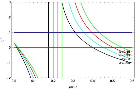
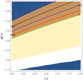
Figure 1: (Color online) On the left panel, the variation of $C_{s}^{2}$ against $\beta B^{2}/2$ is shown, while on the right panel, the contour plots in plane of $\beta B^{2}/2$ and $2\alpha$.

On the left panel, for $0.25<\alpha<0.4$ we see that $0<C_{s}^{2}\leq 1$. While on the right panel, we see that $0<C_{s}^{2}<1$ for $0.25<\alpha<0.4$ and $0.6<\beta B^{2}<1$. This suggests that the model is classically stable and it’s causality is respected in some region of the parameter space. In the remaining part of our analysis, we will confine ourselves in these regions of $\alpha$ and $\beta B^{2}$.
In Fig. (2), we have plotted the equation of state parameter $\omega$ against $\beta B^{2}/2$ for different $\alpha$

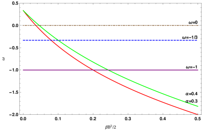
Figure 2: (Color online) Plot showing the variation of $\omega$ against $\beta B^{2}/2$.

From the Fig. (2), we find that Universe has large negative EoS for small a( large $\beta B^{2}$) and it crosses $\omega=-1$ at $\beta B^{2}=0.4(0.5)$ corresponding to $\alpha=0.3(0.4)$, while for $\omega=-1/3$ and $\alpha=0.3(0.4)$, we find $\beta B^{2}=0.15(0.2)$, respectively. Universe changes from acceleration to deceleration phase.In the limit $\beta B^{2}\rightarrow 0$, $\omega$ approaches 1/3( radiation dominated Universe). Next, we define the deceleration parameter($q$) as

$$q=-\frac{a\ddot{a}}{\dot{a}^{2}}=\frac{1}{2}(1+3\omega)=\frac{2\alpha-3\beta B^{2}-2\alpha\beta B^{2}-\beta^{2}B^{4}}{2\alpha+\beta B^{2}}$$ (19)

In Fig. (3), on the left panel, we have shown how the deceleration parameter $q$ varies with $\beta B^{2}$ for $\alpha=0.3$, while on the right panel, we have made a contour plot in the $\beta~{}-~{}B$ plane corresponding to $q=0.5,0$ and $-1$ (which corresponds to $\omega=0,~{}-1/3$ and $-1$), respectively.

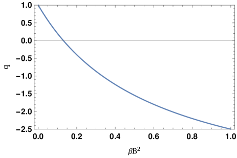
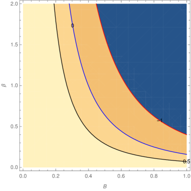
Figure 3: (Color online) Plot showing the variation of $q$ against $\beta B^{2}$ corresponding to $\alpha=0.3$.

From the Fig. (3), we find that the deceleration parameter $q$ remains negative so long $\beta B^{2}\geq 0.28$ (for $\alpha=0.3$) which implies the accelerating phase of the universe expansion.

From the velocity (Friedmann) equation (for $k=0$ case(flat universe)), we find

$$H^{2}=\left(\frac{\dot{a}}{a}\right)^{2}=\frac{\rho_{B}}{3}$$ (20)

we obtain the equation which shows the conservation of energy with effective potential $V_{eff}(a)$,

$$\dot{a^{2}}+V_{eff}(a)=0$$ (21)

In above, $V_{eff}(a)=-\frac{B_{0}^{2}}{6a^{2}}e^{-\beta B_{0}^{2}/2a^{4}}\left(\frac{\beta B_{0}^{2}}{2a^{4}}+\alpha\right)^{-2}$ where we have used $B=B_{0}/a^{2}$. In Fig. (4), on the left panel, we have plotted $V_{eff}(a)$ as a function of $a$ for $\beta=0.4$ and $\alpha=0.3$.

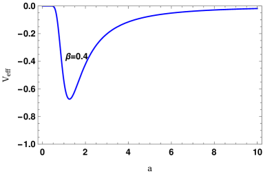
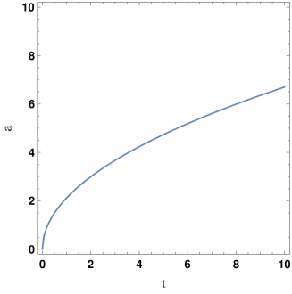
Figure 4: (Color online) On the left panel, plot showing the variation of $V_{eff}$ against $a$ for $\alpha=0.3$ and $\beta=0.4$, while on the right panel, $a(t)$ is plotted against $t$.

We see that for the entire range of values of $a$, $V_{eff}$ always remain negative, which suggests that $\dot{a}^{2}>0$ throughout. For small $B=\frac{B_{0}}{a^{2}}$ due to large $a$, we obtain (from Eq. 21) $\dot{a^{2}}=\frac{B_{0}^{2}}{6\alpha^{2}a^{2}}$. Integrating we get, $t-t_{0}=\sqrt{\frac{3\alpha^{2}}{2B_{0}^{2}}}~{}a^{2}$ where $t_{0}$ is the integration constant. Setting $t_{0}=0$, the present time and $B_{0}=1$ (the present day normalized magnetic field value), we find (with $\alpha=1$)

$$a=\left(\frac{2}{3}\right)^{1/4}\left(\frac{t}{\alpha}\right)^{1/2}$$ (22)

A plot showing the variation of $a(t)$ against $t$ is shown on the right panel of Fig. 4 and the behaviour of $a(t)$ as a function of $t$ is as per the normal electrodynamics, since in the limit $\alpha\to 1$, ${\mathcal{L}}_{NED}\to-{\mathcal{F}}$, the usual QED lagrangian. Note that at $t=0,a_{0}=0$, the function $a_{0}$ is the radius of Universe which shows that Universe begins from the zero point. Similarly, the acceleration (the Raychaudhury) equation gives,

$$\ddot{a}+W_{eff}=0$$ (23)

Where $W_{eff}=-\frac{B_{0}^{2}}{12a^{3}}e^{-\beta B_{)}^{2}/2a^{4}}\left(\alpha+\frac{\beta B_{0}^{2}}{2a^{4}}\right)^{-3}\left[\frac{\beta^{2}B_{)}^{4}}{a^{8}}+\frac{\beta B_{0}^{2}}{a^{4}}\left(2\alpha+3\right)-2\alpha\right]$.

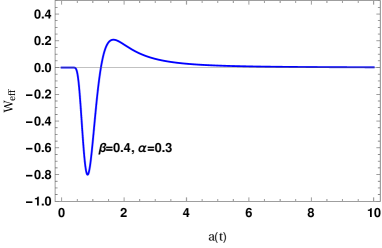
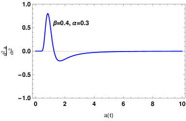
Figure 5: (Color online) Plots showing the variation of $V_{eff}$ against $a$(on the left panel) and $\ddot{a}$ against $a(t)$(on the right panel) corresponding to $\alpha=0.3,\beta=0.4$.

On the left panel of Fig. (5), we have plotted $W_{eff}$ against $a$, while on the right panel $\ddot{a}(t)$ is shown as a function of $a(t)$ corresponding to $\alpha=0.3$ and $\beta=0.4$. We see that as long as $W_{eff}$ remains negative, the universe accelerates i.e. $\ddot{a}(t)>0$. Accordingly, one finds the magnetic field which evolves as

$$B(t)=\frac{B_{0}}{a^{2}}=\frac{\alpha\sqrt{6}}{2}\frac{1}{t}$$ (24)

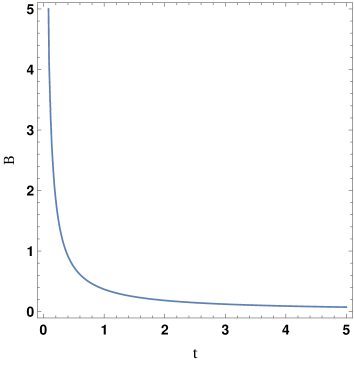
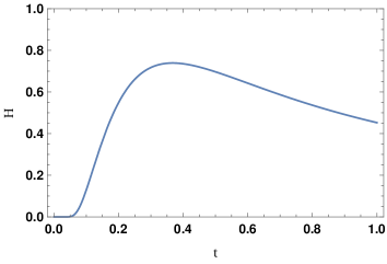
Figure 6: (Color online) On the left, $B(t)$ is plotted against $t$, while on the right the Hubble parameter $H(t)$ is plotted as a function of $t$ with $\alpha=0.3$.

Using Eq. (20), one finds Hubble parameter $H$ varies with $t$ as

$$H=\frac{\alpha e^{-\left(\frac{3\alpha^{2}\beta}{8t^{2}}\right)}}{t\left(2\alpha+\frac{3\alpha^{2}\beta}{2t^{2}}\right)}\to\frac{1}{2t}$$ (25)

in the limit $\alpha\to 1$ and $\beta\to 0$. The plots showing the variation of $B(t)$ against $t$ and $H(t)$ against $t$ are shown in Fig.6.

Also during inflation, one finds $\dot{\rho_{B}}=0$ (from the equation of continuity) i.e. $\rho_{B}$ = constant (as $\rho_{B}+P_{B}=0$) and this gives

$$\beta^{2}B^{4}+\beta B^{2}(2+2\alpha)-4\alpha=0$$ (26)

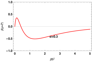
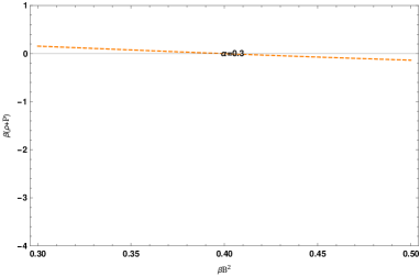
Figure 7: (Color online) Plot showing the variation of $\beta(\rho+3P)$ against $\beta B^{2}$ with $\alpha=0.3$.

From the above equation, we get $\beta B^{2}=0.4$ for $\alpha=0.3$, which is found to be consistent with Fig. (7) where we have plotted $\beta(\rho_{B}+P_{B})$ against $\beta B^{2}$. Using this $\beta B^{2}=0.4$ value in Eq. (26), one finds the maximum energy density $\rho_{B}$ occurs at

$$\rho_{B}=\frac{2\beta B^{2}e^{-\beta B^{2}/2}}{\beta(2\alpha+\beta B^{2})^{2}}=0.65/\beta=\rho^{max}_{B}~{}\to\beta\rho^{max}_{B}=0.65$$

where we have set $\alpha=0.3$. Note that $\rho_{B}(=\rho^{max}_{B})$ remains constant during inflation. This energy density $\rho_{max}$ gives the value of the magnetic field $B\simeq\sqrt{\frac{0.4}{\beta}}=\sqrt{\frac{0.4\rho^{max}_{B}}{0.65}}$ for the inflationary phase. In a typical inflationary model (e.g. chaotic, hybrid, natural) where the reheating temperature is $T_{reh}\sim\rho_{inf}^{1/4}\sim 10^{16}~{}\rm{GeV}$, i.e. at grand unification scale, the energy density during inflation is taken to be $\rho_{inf}(=\rho^{max}_{B})=10^{64}~{}\rm{GeV^{4}}$. Accordingly, we find the magnetic field to be at the beginning,

$$B_{start}=\sqrt{\frac{0.4(=\rho^{max}_{B})}{0.65}}=0.79\times 10^{32}\frac{1}{2\times 10^{-20}}G=0.395\times 10^{52}\sim 4\times 10^{51}G$$ (27)

In Fig. (8), we have plotted the scale factor $a$ (where $a=\frac{1}{1+z}$) as a function of the redshift factor $z$. We see that as $z\rightarrow 0$, the scale factor $a$ increases to a very large value corresponding to the current universe, whereas as $z\to$ large value (corresponding to early day universe), $a\rightarrow 0$.

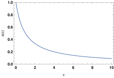
Figure 8: (Color online)Plot showing the variation of $a(z)$ against $z$.

In Fig. (9), we have shown how the magnetic field $B$ evolves with $z$. We see that as $z$ increases from $0$(present day value) to $1089$ (the redshift value corresponding to the event of first CMBR formation) and further to extremely high value $10^{29}$ (the redshift value corresponding to the event inflation), $B$ varies from a very small value $10^{-10}$ G (present day value) to $10^{-4}$ G (the value at the time of CMBR formation) and then to $\sim 10^{51}$ G, the very $B$ value necessary to trigger inflation.

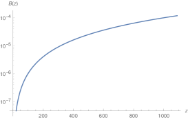
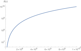
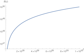
Figure 9: (Color online)Plots showing the variation of $B(z)$ (in Gauss(G)) against $z$. On the extreme left, $z$ varies from $0$ to $1089$, in the case of middle one $z$ varies from $1089$ to $10^{10}$, whereas on the extreme right, $z$ varies from $10^{10}$ to $10^{30}$.

Noting, if inflation scale is determined by the reheating temperature $T=10^{16}~{}\rm{GeV}=5\times 10^{29}\rm{cm^{-1}}\approx 1/a$, one finds $a=0.2\times 10^{-29}\rm{cm}$, and $z=5\times 10^{29}$ which corresponds to $B(t=t_{in}=10^{-36}~{}\rm{sec})=B_{0}(1+z)^{2}\approx 3\times 10^{49}$ G, a value close to our earlier estimate of $B\sim 10^{51}$ G.
e-fold number(N):  The e-fold number($N$) in terms of the magnetic field $B$ is defined by

$$N=\ln\frac{a_{end}}{a_{start}}=\ln{\sqrt{\frac{B_{start}}{{B_{end}}}}}$$ (28)

Considering, $B_{0}\simeq B_{end}=10^{-10}$ G (corresponding to $z=0$) and $B_{start}=4\times 10^{51}$ G, we find $N=\frac{1}{2}\times\ln({4\times 10^{61}})=71$ (whereas for $B_{start}=3\times 10^{49}$ G, we find $N=69$). Also, if we consider $B_{end}=10^{-4}$ G (corresponding to $z=1089$) and $B_{start}=4\times 10^{51}$ G, we find $N=\frac{1}{2}\times\ln({4\times 10^{55}})=64$ (whereas for $B_{start}=3\times 10^{49}$ Gauss, we find $N=62$). This agrees quite well with the experimental result.

4 Conclusion:

In this paper we have considered a new kind of NLED field which acts as a source of gravity and can accelerate the universe to accelerate during the inflationary era. We have studied the isotropic and homogeneous magnetic universe where the newly proposed NLED lagrangian is charecterized by two paremetrs $\alpha$ (dimensionaless parameter) and $\beta$ (dimensionful parameter). We have investigated the classical stability and causality aspects of our model of inflationary expansion by demanding that the speed of the sound wave $C_{s}^{2}>0$ and $C_{s}\leq 1$. We found that $0<C_{s}^{2}<1$ for $0.25\leq\alpha\leq 0.4$ and $0.6\leq\beta B^{2}\leq 1$. A plot of $\omega$(equation of state parameter $=P/\rho$) against $\beta B^{2}/2$ for $\alpha=0.3$ suggests that $0.2\leq\beta B^{2}\leq 0.4$ provided $-1/3\leq\omega\leq-1$. The deceleration parameter($q$) study also suggests that $q<0$ (i.e. $\omega<-1/3$ with $q=\frac{1}{2}(1+3\omega)$) and hence $\ddot{a}>0$ ( the universe is accelerating) provided $\beta B^{2}\geq 0.13$. During inflation, the energy density $\rho_{B}$ is found to be maximum and is given by $\rho_{B}^{max}=0.65/\beta$. The magnetic field necessary to trigger the inflation, is found to be $B\simeq\sqrt{\frac{0.4\rho_{B}^{max}}{0.65}}=4\times 10^{51}~{}{\rm Gauss}$, where $\rho_{B}^{max}(\sim\rho_{inf})=10^{64}~{}{\rm GeV}^{4}$ is the energy density of the universe during inflation and we found that the field $B$ decreases with time $t$. Our model also predicts the e-fold number $N=71(64)$ that the magnetic field at the end of inflation is about $B=10^{-10}~{}(10^{-4})$ Gauss corresponding to $z=0(1000)$ and this agrees quite well with the experimental prediction of the e-fold number. We found that our model describes several aspects of inflationary cosmology and is classically stable in a range of parameters($\alpha,\beta$) space.

5 Acknowledgement

PS thanks to Department of Science and Technology, Government of India for the Inspire fellowship (No. DST/INSPIRE Fellowship/2017/IF170807). The work of PKD and GCS is supported by CSIR Grant No.25(0260)/17/EMR-II

References

- [1] E. Kolb and M. S. Turner, The Early Universe, CNC Press, 1994.
- [2] The Nobel Prize in Physics 2011. NobelPrize.org. Nobel Media AB 2019. Wed. 5 Jun 2019. https://www.nobelprize.org/prizes/physics/2011/summary/.
- [3] Supernova Search Team Collaboration, A. G. Riess et al. Astron. J. 116 (1998) 1009 - 1038.
- [4] Supernova Cosmology Project Collaboration, S. Perlmutter et al.,Astrophys. J. 517 (1999) 565 - 586.
- [5] S. M. Carroll, Living Rev. Rel. 4 (2001) 1, arXiv:astro-ph/0004075 [astro-ph].
- [6] P. Peebles and B. Ratra, Rev. Mod. Phys. 75 (2003) 559 - 606, arXiv:astro-ph/0207347 [astro-ph].
- [7] D. Baumann, TASI Lectures on Inflation, arXiv:0907.5424v2 [hep-th].
- [8] S. Nojiri and S. D. Odintsov, Phys. Rep. 505 (2011) 59 - 144.
- [9] T. Clifton et. al , Phys. Rep. 513 (2012) 1 - 189.
- [10] Övgün, Ali and Leon, Genly and Magaña, Juan and Jusufi, Kimet,The European Physical Journal C 78 (2018), [arXiv:1709.09794]
- [11] S. I. Kruglov, Annals Phys 353 (2014) 299.
- [12] S. I. Kruglov, Phys. Rev. D 92 (2015) 123523.
- [13] S. I. Kruglov, Phys. Rev. D 92 (2015) 123523.
- [14] J. D. Jackson, Classical Electrodynamics, Second Ed. John Wiley and Sons, 1975.
- [15] M. Born and L. Infeld, Proc. Royal Soc. (London) A 144 (1934) 425.