Identifying tracé alternant activity in neonatal EEG using an inter-burst detection approach

Abstract

Electroencephalography (EEG) is an important clinical tool for reviewing sleep–wake cycling in neonates in intensive care. Tracé alternant (TA)—a characteristic pattern of EEG activity during quiet sleep in term neonates—is defined by alternating periods of short-duration, high-voltage activity (bursts) separated by lower-voltage activity (inter-bursts). This study presents a novel approach for detecting TA activity by first detecting the inter-bursts and then processing the temporal map of the bursts and inter-bursts. EEG recordings from 72 healthy term neonates were used to develop and evaluate performance of 1) an inter-burst detection method which is then used for 2) detection of TA activity. First, multiple amplitude and spectral features were combined using a support vector machine (SVM) to classify bursts from inter-bursts within TA activity, resulting in a median area under the operating characteristic curve (AUC) of 0.95 (95% confidence interval, CI: 0.93 to 0.98). Second, post-processing of the continuous SVM output, the confidence score, was used to produce a TA envelope. This envelope was used to detect TA activity within the continuous EEG with a median AUC of 0.84 (95% CI: 0.80 to 0.88). These results validate how an inter-burst detection approach combined with post processing can be used to classify TA activity. Detecting the presence or absence of TA will help quantify disruption of the clinically important sleep–wake cycle.

I Introduction

Sleeping is the primary activity of newborns. Disturbances to the sleep–wake cycle can provide valuable insights into neurological development and maturation [1]. Electroencephalography (EEG) provides a continuous measurement of electrical brain activity that is well suited to analysing sleep–wake cycling in the neonate [1]. But around-the-clock EEG monitoring and review in most neonatal intensive care units (NICU) is not practical. Automated EEG analysis could help by presenting the physician with useful and timely clinical information about brain function.

Sleep–wake cycling is evident in healthy term neonates within hours of birth [1]. This cycle can be classified into 4 behavioural states: active sleep, quiet sleep, indeterminate sleep, and wakefulness. Quiet sleep itself consists of 2 different EEG patterns, high-voltage slow wave ($<$4 Hz) activity and tracé alternant (TA) activity. TA activity is characterised by high voltage waveforms, typically 50 to 150 $\mu$V peak-to-peak, separated by lower-voltage waveforms, typically between 25 to 50 $\mu$V peak-to-peak [2]. We refer to the higher voltage activity as bursts and the lower voltage activity as inter-bursts. Each waveform lasts from a few seconds up to approximately 10 seconds [2].

There has been a limited amount of work on automating the detection of different sleep states in neonatal EEG. Dereymaeker et al. [3] presented a method to detect quiet sleep and active sleep for preterm infants. Both Pillay et al. [4] and Ansari et al. [5] developed different methods to detect components of quiet and active sleep states, including TA activity, using a combined cohort of preterm and term infants with EEG recorded at term-equivalent age. Turnbull et al. [6] focused solely on detecting TA activity in term EEG. This study explored the potential for using the discrete wavelet transform, using a small dataset of 20 EEG segments from 6 neonates.

As TA activity is an essential component of quiet sleep, it is therefore an important neurophysiological marker of normal function and maturation [7, 1]. We aim to develop a method that detects the presence or absence of TA activity within an EEG recording. TA activity, with its quasi-periodic sequence of bursts and inter-bursts, contrasts sharply with other EEG activity. To develop the TA detector, we first construct a detector to differentiate between bursts and inter-bursts. Next, we process the output of the burst–inter-burst detector and use this processed envelope to distinguish between TA activity and non-TA activity in the continuous EEG. We intend to use this TA module as part of an algorithm that grades neonatal EEG for hypoxic ischemic encephalopathy described in [8]. A TA activity detector, combined with a grading algorithm [8], could help distinguish normal from abnormal EEG.

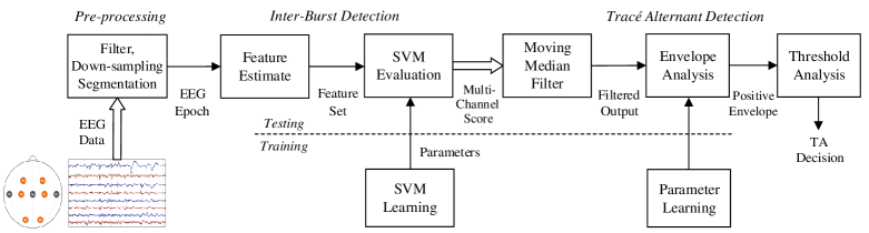
Figure 1: Overview of proposed system for detecting tracé alternant activity. SVM: support vector machine; TA: tracé alternant.

II Methods

We first develop an automated method to segment TA activity into bursts and inter-bursts. We do this by extracting multiple features and combine using a machine learning method. Second, we process the classifier’s decision function when applied to the whole EEG, which includes both TA and non-TA activity, to generate a score to detect TA. The overall structure of the proposed system is shown in Fig. 1.

II-A EEG Data and Pre-processing

EEG was recorded from term infants using a NicoletOne EEG system in Cork University Maternity Hospital, Cork, Ireland. Informed and written parental consent was obtained before EEG recording. The study was approved by the Clinical Ethics Committee of the Cork Teaching Hospitals. EEG recordings started as soon as possible after birth and continued for up to 1–2 hours to include different sleep states. Five scalp electrodes were used over the frontal and temporal regions with reference in the midline (Cz). We analysed the EEG using a 4-channel bipolar montage, derived from these electrodes as F3-T3, F4-T4, T4-Cz and Cz-T3.

A subset of 72 EEGs, from a total of 91 EEGs, were selected for this study based on presence of $>$2 min of continuous TA activity. This dataset is detailed in Korotchikova et al. [1]. An EEG expert reviewed and annotated instances of TA activity [1]. Within the TA activity all bursts and inter-bursts were also annotated. Fig. 2 shows an example of annotated bursts and inter-bursts for 1 channel.

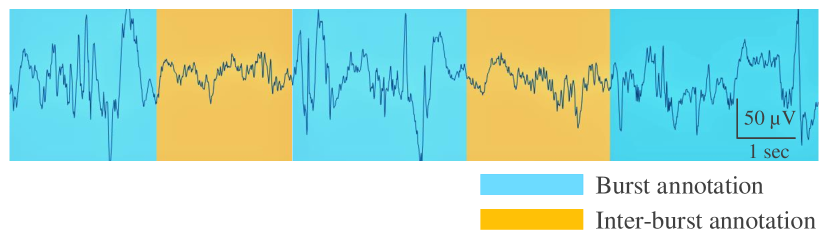
Figure 2: Annotations of bursts and inter-bursts within tracé alternant activity for 1 channel of EEG.

EEG data were sampled at 256 Hz during recording and electrode impedance was maintained below 5 k$\Omega$. Movement artefacts, defined as the absolute value of EEG $>$1,500 $\mu$V, were removed. EEG was low-pass filtered to 30 Hz using an finite-impulse response (FIR) filter of length 4,001 samples and then down-sampled to 64 Hz.

II-B Burst and Inter-burst Detection

As part of the proposed system, we first developed a method to classify bursts and inter-bursts present within TA activity. Because TA activity is a maturation of the tracé discontinue activity present in preterm EEG, we started by modifying a feature set developed to detect bursts and inter-bursts in preterm EEG [9]. These features capture differences in amplitude and spectral shape across four modified frequency bands 0.5–4 Hz, 4–7 Hz, 7–13 Hz, and 13–30 Hz, and one frequency-weighted energy measure called the envelope–derivative operator within the 0.5–10 Hz band [10]. EEG signals $x(n)$ are bandpass filtered into the $i$-th frequency band using a 5th-order Butterworth filter, resulting in $x_{i}(n)$. The filters are implemented using a forward–backwards procedure to obtain a zero-phase response [9]. The features are defined, for finite signal $x_{i}(n)$ of length $N$, as follows.

1. Envelope: quantifies power in the signal by computing the median of the signal envelope $e_{i}(n)$. The envelope is defined as

$$e_{i}(n)=|z_{i}(n)|^{2}=|x_{i}(n)+jH[x_{i}(n)]|^{2}$$ (1)

where $z_{i}(n)$ is the analytic associate of $x_{i}(n)$, $H[\cdot]$ represents the Hilbert transform, and $j$ represents the imaginary unit.

2. Fractal dimension: time-domain approach to quantify the complexity of the signal. Here we use the Higuchi method, which first estimates curve length at the $k$th-scale as,

$$L_{m}(k)={} \dfrac{(N-1)}{\lfloor(N-m)/k\rfloor k^{2}}\;\;\times$$ (2)

$$\sum_{i=1}^{\lfloor(N-m)/k\rfloor}|x[m+ik]-x[m+(i-1)k]|$$

over $m=1,2,...,k$ using the entire frequency range 0.5–30 Hz. Curve length $L(k)$, at scale $k$, is then computed as the mean value of $L_{m}(k)$ over all $m$ values. This process is iterated for different scale values $k$. The slope of a line fit to the points (log $k$, log $L(k)$) provides an estimate of fractal dimension.

3. Relative spectral power: quantifies spectral shape by assessing the relative power of the $i$-th frequency band,

$$P_{i}=\dfrac{\sum_{k\in i}|X(k)|^{2}}{P_{\text{total}}}$$ (3)

where $X(k)$ is the discrete Fourier transform (DFT) of $x(n)$, $P_{\text{total}}$ is the total spectral power over the 0.5–30 Hz range, and notation $\sum_{k\in i}$ represents summation over the $i$-th frequency band.

4. Measure of spectral fit: also quantifies spectral shape. The line $\widehat{Y}(l)=c_{1}+c_{2}l$ approximates the log–log spectrum $Y(l)$ and measure of fit $r^{2}$, defined as

$$r_{i}^{2}=1-\dfrac{\sum_{l\in i}\left[Y(l)-\widehat{Y}(l)\right]^{2}}{\sum_{l\in i}\left[Y(l)-\dfrac{1}{N_{i}}\sum_{l\in i}Y(l)\right]^{2}}$$ (4)

is used as the feature. $Y(l)$ is the log of $|X(k)|^{2}$ at log frequency $l$. Each $i$-th frequency band is fitted separately.

5. Instantaneous frequency: yet another feature that quantifies spectral shape. The feature is computed as the median of the instantaneous frequency $f_{i}(n)$, where $f_{i}(n)$ is estimated using the central-finite difference as,

$$f_{i}(n)=\dfrac{f_{s}}{4\pi}\left\{\left[\phi_{i}(n+1)-\phi_{i}(n-1)\right]~{}\text{mod}~{}2\pi\right\}$$ (5)

with phase function $\phi_{i}(n)=\text{arg}[z_{i}(n)]$, where $z_{i}(n)$ is the analytic signal from (1) for the $i$-th frequency band.

6. Envelope–derivative operator: quantifies the frequency-weighted energy of the signal. This non-negative measure combines both amplitude and frequency as [10],

$$\Gamma(n)=\dfrac{1}{4}[x^{2}(n+1)+x^{2}(n-1)+h^{2}(n+1)+h^{2}(n-1)]+\\ [x(n+1)x(n-1)+h(n+1)h(n-1)]$$ (6)

where $h(n)=H[x(n)]$ is the Hilbert transform of $x(n)$.

Features 1 to 5 are generated on short-duration epochs with 75% overlap. Time-domain features (1 and 2) use 1-second epochs; spectral features (3, 4, and 5) use 2-second epochs. The envelope–derivative operator (feature 6) is computed on the whole signal. Features 1, 3, 4, and 5 are computed for the 4 different bands, resulting in a total of 18 features. Feature selection criteria of an area-under the operating characteristic curve (AUC) $>$0.6 was implemented for each feature individually within a leave-one-subject-out (LOSO) cross-validation.

This feature set was combined using a linear support vector machine (SVM), in keeping with the preterm burst-detection method on which this feature set is based [9]. In addition, 2 other models were tested: a Fisher discriminate analysis model and a random forest model. The random forest hyper-parameters—number of trees and maximum number of levels in each decision tree—were selected within a nested cross-validation scheme. We also implemented a radial basis function SVM but found little difference in performance during initial testing compared to the linear SVM and therefore we only consider the linear SVM here.

Computer code (Matlab) for the inter-burst detector trained on all EEG records is available at https://github.com/sumitraurale/interburst_detector.

II-C TA Detection

We use the continuous-valued output of the burst detector, the confidence score, to differentiate TA activity from other EEG activity. The process is as follows. First, we apply a low-pass smoothing process to the score to suppress the higher-frequency noise and outliers. For this we use a 3-second moving-median filter. We produce a summarised filtered score by averaging across channels. Second, we then apply an envelope estimation method to the filtered confidence score. Local maxima are computed on the score with a parameter that specifies the minimum separation between consecutive peaks. These peaks are then joined using spline interpolation to create a smooth envelope function. This envelope is in turn a confidence score of the presence or absence of TA activity. The minimum separation parameter for the local maxima is optimised during training over the range (2.5, 50) seconds with step size of 2.5-seconds. Each EEG is segmented into 20 minute epochs and only those epochs with either full TA activity or full non-TA activity are considered. Fig. 3 shows an example of the filtered confidence score from the burst detector and the envelope, highlighting the smoothing effect of the envelope estimation process.

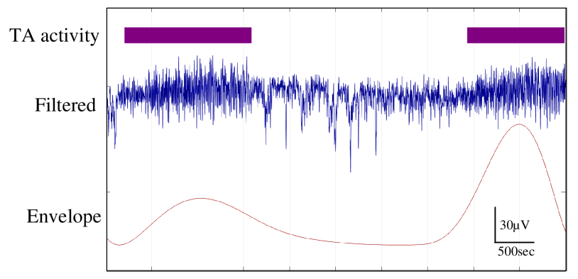
Figure 3: TA envelope for 1.3 hours of EEG. Filtered confidence score from the inter-burst detector and smoothed envelope function depicted in relation to TA activity.

For training and testing the inter-burst and TA detector, we use LOSO cross-validation. Feature selection for the inter-burst detector and parameter optimisation for the TA envelope method is generated within the LOSO cross-validation.

III Results

The same feature set of 9 features were selected at each of 72 LOSO iterations. Individual feature performance for these features are illustrated in Fig. 4 based on an AUC for each EEG record.

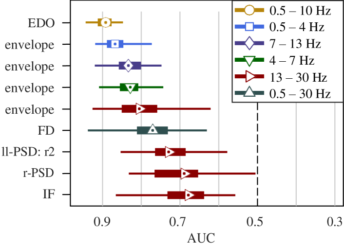
Figure 4: Detection performance for individual features of the inter-burst detector, calculated in different frequency bands. Dots represent median values, thick lines inter-quartile range, and thin lines 95th percentile range of AUC values for the 72 infants. EDO: envelope–derivative operator; r-PSD: relative power spectral density (PSD); ll-PSD: r2: linear fit ($r^{2}$) to log–log PSD; IF: instantaneous frequency; FD: fractal dimension.

AUC values, comparing classifiers, for the inter-burst detection component of the proposed system are illustrated in Table I. Although there is little difference in performance the linear SVM outperforms both the FDA and random forest classifiers. Thus we proceeded with this SVM to generate the TA envelope and detector.

TABLE I: Performance for detecting bursts and inter-bursts with tracé alternant activity using 3 different classifiers.

	FDA	Random Forest	Linear-SVM
Median AUC	0.91	0.91	0.92

FDA: Fisher discriminant analysis; SVM: support vector machine

Testing performance of the inter-burst detector improves when a decision is made over the 4 channels. For a single channel, median AUC is 0.92 (95% confidence intervals, CI: 0.90 to 0.97) compared to a median AUC of 0.95 (95% CI: 0.93 to 0.98) from averaging the confidence score over all channels.

The post-processed envelope function is then tested to detect the presence of TA activity. Table II presents the performance metrics for testing the TA detector using the held-out testing inter-burst detector model from the LOSO cross-validation. A threshold value of 2.06 on the envelope function gives approximately equal sensitivity and specificity (76.2% and 76.3%).

TABLE II: Classification performance for the proposed TA detector.

Cohen’s	AUC	F1-score	Accuracy
kappa	(95% CI)	(%)	(%)
0.57	0.84	79.7	81.9
	(0.80, 0.88)

Key, AUC: Area-under receiver operating characteristic; CI: confidence interval.

IV Discussion and Conclusions

We present a novel approach for detecting tracé alternant in the EEG of term neonates by first developing a burst–interburst detector and then post-processing this detector’s confidence score. The method is trained and tested on a large EEG database from 72 term infants EEG, recorded within days of birth. The inter-burst detector, which combines amplitude and spectral characteristics using a machine learning approach, results in an AUC of 0.95 (95% CI: 0.93 to 0.98). This detector is used to evaluate the presence of inter-burst intervals by generating an envelope which detects TA activity with reasonable performance ($\kappa=0.57$, F1 = 79.7%, accuracy = 81.9%, and AUC = 0.84).

It is difficult to directly compare our results to other studies. Most use EEG from both preterm and term infants [3, 5], with some of the term EEG from infants born preterm [4, 11]. The distinction in our work is that we developed our methods on EEG recorded within days of birth from a healthy cohort of term infants. Also, most methods focus on classifying different sleep states, such as active sleep and quiet sleep. Here we focus solely on TA activity, a subset of quiet sleep. Probably the most similar study to ours was presented by Turnbull et al. [6], but the lack of detection results prevents direct comparison.

In conclusion, we have developed a method to detect TA activity in the EEG of term neonates. By enabling simple spatio-temporal post-processing analysis on the burst–interburst sequence we generate promising system performance. Future work will investigate developing statistical features, in conjunction with machine learning methods, of the temporal organisation of the burst–interburst sequence to further improve classification performance. The proposed method could help highlight disturbances to the sleep–wake cycle by noting the presence or absence of TA activity and therefore help identify neurologically compromised infants, such as those with hypoxic-ischemic encephalopathies.

References

- [1] I. Korotchikova, N. J. Stevenson, V. Livingstone, C. A. Ryan, and G. B. Boylan. “Sleep–wake cycle of the healthy term newborn infant in the immediate postnatal period” Clinical Neurophysiology, vol. 127. no. 4, pp. 2095–2101, 2016.
- [2] T. N. Tsuchida, et al. “American clinical neurophysiology society standardized EEG terminology and categorization for the description of continuous EEG monitoring in neonates: report of the American Clinical Neurophysiology Society critical care monitoring committee.” Journal of Clinical Neurophysiology, vol. 30, no. 2, pp. 161-173, 2013.
- [3] A. Dereymaeker, K. Pillay, J. Vervisch, S. Van Huffel, G. Naulaers, K. Jansen, and M. De Vos, “An automated quiet sleep detection approach in preterm infants as a gateway to assess brain maturation” Journal of Neural Systems, vol. 27, no. 06, 2017.
- [4] K. Pillay, A. Dereymaeker, K. Jansen, G. Naulaers, S. Van Huffel, and M. De Vos, “Automated EEG sleep staging in the term-age baby using a generative modelling approach” Journal of Neural Engineering, vol. 15, no. 03, 2018.
- [5] A. H. Ansari, O. De Wel, K. Pillay, A. Dereymaeker, K. Jansen, S. Van Huffel, G. Naulaers, and M. De Vos, “A convolutional neural network outperforming state-of-the-art sleep staging algorithms for both preterm and term infants” Journal of Neural Engineering, vol. 17, no. 03, 2020.
- [6] J. P. Turnbull, K. A. Loparo, M. W. Johnson, and M. S. Scher, “Automated detection of tracé alternant during sleep in healthy full-term neonates using discrete wavelet transform” Clinical Neurophysiology, vol. 112, no. 10, pp. 1893–1900, 2001.
- [7] A. Dereymaeker, K. Pillay, J. Vervisch, M. De Vos, S. Van Huffel, K. Jansen, and G. Naulaers, “Review of sleep-EEG in preterm and term neonates” Early Human Development, vol. 113, pp. 87–103, 2017.
- [8] S. A. Raurale, S. Nalband, G. B. Boylan, G. Lightbody, and J. M. O’Toole, “Suitability of an inter-burst detection method for grading hypoxic-ischemic encephalopathy in newborn EEG” in 41st International Conference on IEEE Engineering in Medicine and Biology Society (EMBC), Germany: IEEE, July 2019, pp. 4125–4128.
- [9] J. M. O’Toole, G. B. Boylan, R. O. Lloyd, R. M. Goulding, “Detecting bursts in the EEG of very and extremely premature infants using a multi-feature approach” Medical Engineering and Physics, vol. 45, pp. 42–50, 2017.
- [10] J. M. O’Toole, A. Temko, N. J. Stevenson, “Assessing instantaneous energy in the EEG: a non-negative, frequency-weighted energy operator” in 36th International Conference on IEEE Engineering in Medicine and Biology Society (EMBC), Illinois: IEEE, 2014, pp. 3288–3291.
- [11] N. Koolen, L. Oberdorfer, Z. Rona, V. Giordano, T. Werther, K. Klebermass-Schrehof, N. Stevenson, and S. Vanhatalo, “Automated classification of neonatal sleep states using EEG”, Clinical Neurophysiology, vol. 128, no. 6, pp. 1100–1108, 2017.