Agglomerative Neural Networks for Multi-view Clustering

Abstract

Conventional multi-view clustering methods seek for a view consensus through minimizing the pairwise discrepancy between the consensus and subviews. However, the pairwise comparison cannot portray the inter-view relationship precisely if some of the subviews can be further agglomerated. To address the above challenge, we propose the agglomerative analysis to approximate the optimal consensus view, thereby describing the subview relationship within a view structure. We present Agglomerative Neural Network (ANN) based on Constrained Laplacian Rank to cluster multi-view data directly while avoiding a dedicated postprocessing step (e.g., using $K$-means). We further extend ANN with learnable data space to handle data of complex scenarios. Our evaluations against several state-of-the-art multi-view clustering approaches on four popular datasets show the promising view-consensus analysis ability of ANN. We further demonstrate ANN’s capability in analyzing complex view structures and extensibility in our case study and explain its robustness and effectiveness of data-driven modifications.

I Introduction

Clustering is a type of unsupervised machine learning techniques that partition data points into groups based on feature similarity. Conventional clustering algorithms [1, 2, 3, 4, 5, 6, 7] are mostly single-view algorithms, which only consider single-source datasets. Therefore, they cannot leverage complex view structures and cannot competently handle complex scenarios. However, many real-world objects contain complex view structures, where each subview carries some unique information and the relationships existing between views may provide complementary information. For instance, when analysing a speech, the fusion of text data, voice data, and the relationships between them is more informative than a single view. Thus, it calls for a multi-view clustering method that can leverage view structures effectively.

Currently, multi-view clustering [8, 9, 10, 11] usually comprises two steps to utilize and fuse view information: geometric consistency (GC) learning and cluster assignment consensus (CAC) learning. GC aims to capture the intrinsic similarity information within a single view; CAC aims to approximate the consensus view, which can combine the diverse similarity information from the subviews in a unified view. Although the existing research has achieved remarkable progress in computer vision, neural language processing and many other fields, there still exist challenges in GC learning and CAC learning.

The first challenge is that most current research fails to combine the advantages of two main kinds of GC learning: compactness-based methods and connectivity-based methods. Compactness-based methods look for distinct representations based on the similarity information (e.g., the eigenvectors of affinity matrix) to embed points [12, 13, 14, 15]. Although they are good at extracting informative embeddings, they need postprocessing (e.g., $K$-means) to obtain the clustering results, which may impair the consistency between the learned representations and the final clustering results. In comparison, connectivity-based GC methods project data and encode the similarity information in connection graphs directly. The connection graphs can assign cluster labels according to the connected components to ensure the consistency between latent representations and the clustering [8, 10, 16, 11]. However, such methods may lose information while embedding raw data to connection graphs directly. It is necessary to propose an extensible data-specific framework that embraces the latent representation learning and clustering consistency simultaneously.

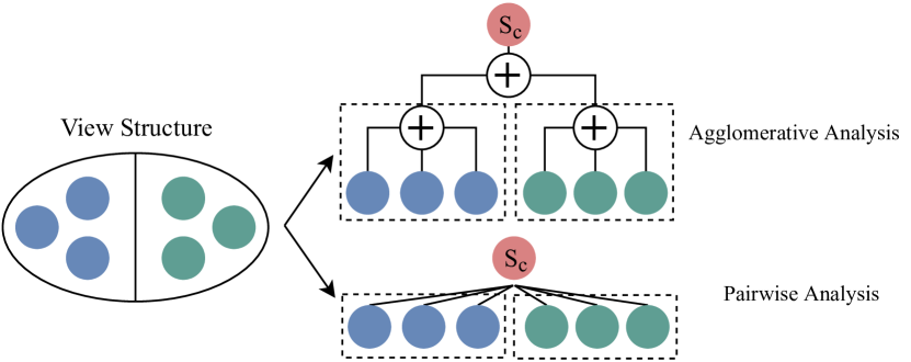
Figure 1: Comparison of pairwise analysis and agglomerative analysis. Given a view structure that contains six independent subviews from two domains (in green and blue, respectively), where each circle represents the information of a subview, pairwise analysis approximates a consensus view $S^{(c)}$ through comparing $S^{(c)}$ with each subview without leveraging the structural information, while agglomerative analysis obtains $S^{(c)}$ by agglomerating subviews following the view structure.

The second challenge is that current CAC research fails to explore view relationships. Most CAC analysis research is inspired by Kumar et al. [12, 13]. The corresponding algorithms rely on pairwise subview comparison [11, 8, 10, 17, 18, 19] to minimize the discrepancy between the consensus view and each subview. Since the pairwise subview comparison methods only analyze the subview independently, they cannot utilize the structural relationship when handling complex hierarchical view structures.

To address the challenges above, we propose agglomerative consensus analysis to portray complex view structures and utilize view relationships. Its difference from the pairwise analysis is illustrated in Fig. 1. Based on the agglomerative consensus analysis, we further propose Agglomerative Neural Network (ANN) to embrace latent representation learning and connectivity-based analysis in a multi-view format. Considering the extensibility of neural networks, we further implement agglomerative consensus analysis through an Agglomerative Neural Network with Learnable Data space (ANNLD). ANNLD introduces data-specific learnable projection to improve the data distribution in ANN.

In summary, we make the following contributions:

• We first propose an agglomerative consensus analysis as a unified framework of latent representation learning and Laplacian rank constrained multi-view clustering, which takes advantages of both compactness-based and connectivity-based GC analysis.

• We present an Agglomerative Neural Network (ANN) to implement agglomerative consensus analysis and adopt its data-specific extension, Agglomerative Neural Network with Learnable Data space (ANNLD), to learn more discriminative projection from entangled data across different views and subviews.

• Our experiments on four commonly used multi-view datasets show ANN’s superiority and robustness in analyzing different multi-view datasets. Our experimental results on Survey dataset demonstrate the excellent performance of ANNLD and extensibility of agglomerative consensus analysis.

II Related Work

The connectivity-based clustering algorithms focus on finding a connection graph to represent raw information and thus directly obtain the clustering results. Therefore, connectivity-based methods may better preserve clustering consistency. Nie et al. [20, 8] proposed to learn the consensus connection graph by comparing it with each subview’s affinity matrix or distance matrix, which used self-weighted subviews to reduce the process of optimization. Since Nie researched on fixed affinity matrices or distance matrices of subviews, Zhan et al. [16] further proposed learnable subview connection graphs and then fused the subviews to obtain the consensus view. Wang et al. [21] proposed to find a fusion view to represent the multi-view information; they further approximate the fusion view by combining weighted subviews under constrained Laplacian rank. Huang et al. [11] learned connection graphs from fixed projected data space and aimed to eliminate the mismatching problem across different views.

The compactness-based methods encoded the clustering information in the eigenvector matrix (or latent representations) and used the postprocessing methods (e.g., $K$-means) to cluster the learned representations. Kumar et al. [12, 13] optimized the eigenvector matrix to contain the clustering indicators and searched for the consensus subview or cross-view by pairwise comparison. Zhang et al. [19] applied matrix factorization and constrained the latent codes to learn the consensus representations in a binary structure. Zhang et al. [22] proposed to learn complementary information from multiple views via constrained tensors. The tensors captured the high order correlation underlying views to reduce cross-view redundancy of the learned subspace representations. Zhou et al. [23] introduced neighbor-kernel-based algorithm that utilized the intrinsic neighborhood structure to preserve the block diagonal structure and to strengthen the robustness against noise and outliers. The algorithm fused these base neighbor kernels to extract a consensus representation through subspace learning.

Moreover, some deep-learning-based algorithms [24, 25, 26] extended the previous work with a non-linear relationship and learned the canonical correlation between views. Wu et al. [27] introduced Markov-chain-based spectral clustering method to find the essential tensor of high order correlation representation. Zhang et al. [28] proposed general relationship learning based on neural networks to learn the pairwise relationship between views and thus obtain the fused view. Huang et al. [29] utilized Siamese network and applied orthogonal constraint to enable network performing local invariance learning and matrix decomposition, which further enhance the pairwise comparison based subspace learning. However, the above algorithms mainly relied on the pairwise comparison between subview and consensus view, so they failed to utilize the view structure information which may provide complementary cross-view information. Besides, few of the mentioned work combined connectivity-based learning and compactness-based in a unified neural network.

Compared to the approaches above, our contributions in this work are two-fold. First, most of the existing approaches only utilize the simple view structure without subdivisions. In contrast, our method specifies more details in the view structure and is capable of dealing with complex hierarchical view structures with subdivisions of subviews. The proposed agglomerative consensus analysis can capture and portray the subdivision relationship when agglomerating subviews. Such agglomerative analysis is more theoretical and effective than conventional consensus analysis in utilizing view information. Second, most current research exclusively studies latent representation for view information, constrained Laplacian matrix, and cross/pairwise consensus view analysis. Little work has been done to incorporate them in a unified framework, and the limited existing studies fail to make a data-specific extension. In comparison, we propose a unified and extensible deep learning-based algorithm that can overcome the above deficiencies.

III Agglomerative Consensus Analysis

Figure 2: An illustration of the proposed ANN. We take an object to show a two-layer view structure consisting of four subviews from two domains. ANN learns the subview information $z^{(v)}$ from $D^{(v)}$ via geometric consistency, converts it into a connection graph $S^{(v)}$, and finally, agglomerates subviews by layers and minimizes the discrepancy in the consensus layer to obtain the clustering result $S^{(c)}$.

This section introduces the methodology and theory to carry out the agglomerative consensus analysis framework for multi-view datasets. The full details of component realization in the neural network will be discussed in Section IV.

The proposed agglomerative loss function comprises three terms:

$$\mathcal{L}=\lambda\mathcal{L}_{sc}+\mathcal{L}_{gc}+\mathcal{L}_{cac}$$ (1)

where $\mathcal{L}_{sc}$ constrains Laplacian matrix rank and controls the clustering convergence; $\lambda$ denotes a weighted parameter; $\mathcal{L}_{gc}$ and $\mathcal{L}_{cac}$ enable the model to learn the multi-view information. To be specific, $\mathcal{L}_{gc}$ encodes the subview information in latent representations by learning geometric consistency; $\mathcal{L}_{cac}$ keeps cluster assignment consistent across views.

III-A Constrained Laplacian Rank for Spectral Clustering

Constrained Laplacian Rank (CLR) loss $\lambda\mathcal{L}_{sc}$, which derives from the spectral clustering, has been a widely used tool to carry out clustering on datasets without any postprocessing. Let $G=(X,S)$ be an undirected graph on $X=[n]$ and the connection graph $S$ be the corresponding edge set. We assume: for any two arbitrary sample point $X_{i}$ and $X_{j}$, $S_{ij}$ carries a non-negative weighted edge to encode the similarity intensity between the points. If there exists a edge between $X_{i}$ and $X_{j}$, $S_{ij}>0$; otherwise, $S_{ij}=0$. Specially, $\forall i\in[n],S_{ii}=0$. We keep the main diagonal element of connection graph equals 0 to ensure the graph is undirected. Further, let $Dg$ be the degree matrix, which is a diagonal matrix $Dg_{ii}=\sum_{j\in[n]}S_{ij},i\in[n]$.

Given $k\in\mathbb{N}$, spectral clustering aims to cut edges with minimum weights and partition $X$ into k clusters. Let $L_{S}=Dg-(S^{T}+S)/2$ denote the unnormalized Laplacian matrix, and spectral clustering solves the cutting problem by minimizing following loss function [30]:

$$\begin{gathered}\min_{H\in\mathbb{R}^{n\times k}}Tr(H^{T}L_{S}H)\\ s.t.\quad H^{T}H=I_{k}.\end{gathered}$$ (2)

where $I$ is the identity matrix and $Tr$ is the trace of matrix. A common solution to $H$ is the eigenvector matrix $F$, which consists of the orthonormal eigenvectors corresponding to the $k$ smallest eigenvalues of $L_{S}$ [31].

Further, we utilize the relationship between eigenvalues and the graph connected components, which can constrain the Laplacian matrix, to directly get clustering results.

Theorem 1.

The multiplicity of the eigenvalue 0 of the Laplacian matrix $L_{S}$ (non-negative) equals the number of the connected components in the connection graph $S$.

Theorem 1 indicates that 0 eigenvalues’ multiplicity equals the cluster number. If there exist $k$ clusters on $X=[n]$, the rank of corresponding Laplacian matrix $L_{S}$ should be $n-k$. Let $\sigma_{i}(L_{S})$ be the $i$th smallest eigenvalues of $L$. According to Ky Fan’s Theorem (Fan 1949), we can relate $F$ to the Laplacian matrix rank

$$\begin{gathered}\mathcal{L}_{sc}=\sum_{i=1}^{k}\sigma_{i}(L_{S})=\min_{F,S}Tr(F^{T}L_{S}F)\\ s.t.\quad F^{T}F=I,rank(L_{S})=n-k\end{gathered}$$ (3)

where $L_{S}$ denotes the corresponding Laplacian matrix of connection graph $S$. The loss function aims to regularize the Laplacian matrix rank to be exactly $n-k$ by minimizing the sum of smallest $k$ eigenvalues to 0. Then, the connection graph will establish $k$ clusters and thus the clustering labels can be directly obtained from $S$.

III-B Agglomerative Multi-view Analysis

This section first clarifies the view structure of the multi-view dataset and then introduces the proposed agglomerative multi-view analysis. The multi-view analysis comprises two parts: $\mathcal{L}_{gc}$ encodes distance information in latent representations by learning GC; $\mathcal{L}_{cac}$ minimizes the discrepancy between the projected connection graph and agglomerated raw information to achieve CAC.

We define $\sim$ as the subview relationship and $\in$ as the belonging relationship. Let $V=\{V^{(0)},V^{(1)},...,V^{(m)}\}$ be a m-layer view structure and $V^{(i)}_{j}$ be the $j$th view in $i$th layer, where $V^{(i)}$ represents the $i$th layer view set. Specially, $V^{(0)}$ consists of the smallest independent subviews and $V^{(m)}$ should only have one member $V^{(m)}_{1}$ to represent the consensus view i.e. the final combined view for the multi-view dataset. Let $v$ be an arbitrary view, say $V^{(i)}_{j}$. For the $0$th layer, we let $\forall v\in V^{(0)}$ be an independent subview belonging to the 0th layer; for any subsequent layer $\forall v\in V^{(i)}$ ($i\geq 1$), we denote the agglomerated view by its corresponding subviews, i.e., $v=\{V^{(i-1)}_{j}:V^{(i-1)}_{j}\sim v\}$, where $\sim$ denotes that $V^{(i-1)}_{j}$ is one of the related subview of $v$ and the relationship is predefined in the dataset. For the ease of illustration, we signify $v^{{}^{\prime}}_{j}$ as the $j$th subview of $v$ and $v=\{v^{{}^{\prime}}_{j}:v^{{}^{\prime}}_{j}\sim v\}$.

Given a m-layer view structure $V$ as above, we assume latent representation $z^{(v)}$ encodes the distance information for each subview $v\in V^{(0)}$. Suppose the corresponding raw information of view $v$ is $D^{(v)}$ (i.e., distance matrix), latent representations $z^{(v)}\in\mathbb{R}^{n\times n}$ minimizes the below loss function to learn GC:

$$\begin{gathered}\mathcal{L}_{gc}=\min_{Z}\sum_{v\in V^{(0)}}\left(\sum D^{(v)}\circ z^{(v)}+\left\|z^{(v)}\right\|_{F}^{2}\right)\\ s.t.\quad Z:=\{z^{(v)}:v\in V^{(0)}\}\end{gathered}$$ (4)

where $\circ$ means Hadamard product. $Z$ denotes the target distance representation set and $z^{(v)}=((z^{(v)})^{T}+z^{(v)})/2$ ensures the distance representations being symmetric.

The first term enables latent representations to encode the raw distance information. The second term is a penalty term to prevent $z_{ij}\rightarrow-\infty$.

We further explain the agglomerative consensus analysis theory. Our goal is to acquire a consensus view $S^{(c)}$ concatenating the multiple view information. It is intuitive to utilize the hierarchical view structure to approximate the fused view layer by layer. Since the fused view information should be related to all the corresponding subviews, we propose our agglomerative analysis by assuming there exists a function $\gamma^{(v)}$ which projects the corresponding subviews to the fused views $v\in V^{(i)}(i\geq 1)$. Given the learned latent representation set $Z:=\{z^{(v)}:v\in V^{(0)}\}$, we assume an activation function $\mathcal{C}(z)\rightarrow S$ can convert representation to an normalized connection graph. Then, we define:

$$S_{v}=\begin{cases}\mathcal{C}(z^{(v)})&\text{ if }v\in V^{(0)}\\ \gamma^{(v)}(\{S^{(v^{{}^{\prime}}_{j})}:v^{{}^{\prime}}_{j}\sim v\})&\text{ if }v\in V^{(i)},i\geq 1\end{cases}$$ (5)

where $v^{{}^{\prime}}_{j}$ is the $j$th corresponding subview $V^{i-1}_{j}$ to compose $v$; $\gamma$ denotes the agglomeration operation. The connection graphs in $V^{(0)}$ are calculated from latent representations and the other graphs are achieved by agglomeration.

We propose an activation function $\mathcal{C}$ to convert latent representations and regularize agglomerated graphs. The activation function ensures that $S$ is a normalized connection graph. Section IV-A elaborates on the activation function and the agglomeration.

Given the consensus connection graph $S^{(c)}$ for a m-layer view structure $V$, we sort the general agglomerated form based on Eq. (5):

$$\begin{gathered}\{S^{(v)}:v\sim V^{(i)}\}=\{\gamma^{(v)}(\{S^{(v^{{}^{\prime}}_{j})}:v^{{}^{\prime}}_{j}\sim v\}):v\sim V^{(i)}\}\\ S^{(c)}=\gamma^{V^{(m)}_{1}}(\{S^{(V^{(m-1)}_{j})}:V^{(m-1)}_{j}\sim V^{(m)}_{1}\})\end{gathered}$$ (6)

Since the last layer will combine all the views of the former layer as a unified view, we let $V^{(m-1)}_{j}$ denote the $j$th subview of the consensus view; $1\leq i<m$.

We hope the consensus connection graph $S^{(c)}$ can learn subview information evenly. Therefore, we also agglomerate distance matrix to achieve the agglomerated consensus raw information $D^{(c)}$:

$$\begin{gathered}\{D^{(v)}:v\sim V^{(i)}\}=\{\sum_{v^{{}^{\prime}}_{j}\sim v}w_{d}^{(v^{{}^{\prime}}_{j})}D^{(v^{{}^{\prime}}_{j})}:v\sim V^{(i)}\}\\ D^{(c)}=\sum_{V^{(m-1)}_{j}\sim V^{(m)}_{1}}w_{d}^{(V^{(m-1)}_{j})}D^{(V^{(m-1)}_{j})}\end{gathered}$$ (7)

where $w_{d}^{(v^{{}^{\prime}}_{j})}=1/|v|,w_{d}^{(V^{(m-1)}_{j})}=1/|V^{(m)}_{1}|$, i.e., the corresponding subview quantity of an agglomerated view.

The consensus raw information $D^{(c)}$ evenly fuses the subview information based on the view structure, and the clustering assignment consensus problem will be converted to minimize the discrepancy between $S^{(c)}$ and $D^{(c)}$. Similarly, we can figure out the loss function for CAC:

$$\begin{gathered}\mathcal{L}_{cac}=\min_{Z,\tau}\sum D^{(c)}\circ S^{(c)}+\left\|S^{(c)}\right\|_{F}^{2}\\ s.t.\quad Z:=\{z^{(v)}:v\in V^{(0)}\},\tau:=\{\gamma^{(v)}:i\geq 1,v\in V^{(i)}\}\\ S^{(c)}=\underbrace{\{{\gamma^{v\in V^{(m)}}(\cdots\{\gamma^{v\in V^{(1)}}(}}_{m\ layers}\{\mathcal{C}(z^{v^{{}^{\prime}}_{j}}):v^{{}^{\prime}}_{j}\sim v\})\})\}\end{gathered}$$ (8)

where $S^{(c)}$ is agglomerated from the converted latent representations layer by layer.

Since $S^{(c)}$ is driven by the agglomerative operation and latent representations, the loss function optimizes $Z,\tau$ to achieve an optimal $S^{(c)}$. Specifically, $\mathcal{L}_{cac}$ approximates such a projection to agglomerate the subviews that can balance making the cross-view solution distribute evenly and optimizing the solution for each subview.

III-C Convergence Analysis

To cluster raw data into $k\in\mathbb{N}$ clusters, $\mathcal{L}$ converges when $rank(L_{S^{(c)}})=n-k$. Consider that $\lambda$ is large enough, $\mathcal{L}\approx\lambda Tr(F^{T}L_{S^{(c)}}F)$. Note that $\forall i,\sigma_{i}(L_{S^{(c)}})\geq 0$, the optimal solution $S^{(c)}$ will let the smallest $k$ eigenvalues be zero.

Lemma 1.

For every vector $f\in\mathbb{R}^{n}$, $f^{T}Lf=\frac{1}{2}\sum_{i,j=1}^{n}S_{ij}(f_{i}-f_{j})^{2}$.

Proof.

The Laplacian matrix definition ensures

$$\begin{split}f^{T}Lf&=f^{T}Dgf-f^{T}Sf=\sum_{1}^{n}Dg_{i}f_{i}^{2}-\sum_{i,j=1}^{n}f_{i}f_{j}S_{ij}\\ &=\frac{1}{2}(\sum_{i=1}^{n}Dg_{i}f_{i}^{2}-s\sum_{i,j=1}^{n}f_{i}f_{j}S_{ij}+\sum_{j=1}^{n}Dg_{j}f_{j}^{2})\\ &=\frac{1}{2}\sum_{i,j=1}^{n}S_{ij}(f_{i}-f_{j})^{2}\end{split}$$

∎

According to Lemma 1, we can directly figure out

$$Tr(F^{T}L_{S^{(c)}}F)=\sum_{1}^{k}\sigma(L_{S^{(c)}})=\frac{1}{2}\sum_{i,j=1}^{n}(F_{ij}-F_{ji})^{2}S^{(c)}_{ij}$$ (9)

Therefore, $\mathcal{L}\approx\frac{\lambda}{2}\sum_{i,j=1}^{n}(F_{ij}-F_{ji})^{2}S^{(c)}_{ij}$. According to the chain rule in neural network, $\mathcal{L}$ keeps monotonically decreasing $S_{ij}$ unless $F_{ij}=F_{ji}$. Since only the 0 eigenvalue’s corresponding eigenvector meets that $\forall i,j,f_{i}=f_{j}$, $\mathcal{L}$ optimizes $Z$ and $\tau$, which drive the optimization of $S^{(c)}$, and keeps cutting the edges to reduce the corresponding eigenvalues until the constrained Laplacian rank $rank(L_{S^{(c)}})=n-k$ can be established. Thus, $\mathcal{L}$ tends to converge.

IV Agglomerative Neural Network

This section introduces Agglomerative Neural Network (ANN) and its extended version, Agglomerative Neural Network with Learnable Data space (ANNLD), as well as their optimization methods.

IV-A Agglomerative Neural Network

The agglomerative consensus analysis relies on the agglomeration operation and constructs the consensus view layer by layer. Since neural networks have a chain structure, we only need to declare the deep learning agglomeration operation as layers in the network. Since conventional neural network only optimizes latent representations according to loss gradient, it may not keep the learned connection graph as normalized. In this regard, we design an activation function $\mathcal{C}$ that regularizes input data to be a normalized connection graph:

$$\mathcal{C}(x_{i})=\begin{cases}\frac{\mathcal{P}\cdot x_{i}-x_{min}}{\mathcal{P}(\sum_{j\in x^{+}}x_{j}-x_{min})}&\text{ if }x_{i}\geq 0\\ \quad\quad\quad 0&\text{ if }x_{i}<0\end{cases}$$ (10)

where $x_{i}$ denotes $i$th element of a row vector $x$. $x_{min},x^{+}$ are the minimum and positive element of vector $x$. $\mathcal{P}$ is a hyper-parameter that prevents the edge from vanishing after rescaling data. The activation function $\mathcal{C}$ plays three roles in the network. First, it regularizes the input vector into a standard affinity vector in the connection graph. It rescales the input vector to $[0,1]$ and lets the sum of elements equal 1. Second, $\mathcal{C}$ also holds inequality relationships between non-negative elements and keeps non-positive edges inactivated to accelerate the optimization. Last, $\mathcal{C}$ can prevent some trivial solutions from cutting one point as a cluster. $\mathcal{C}$ tends to keep the last positive edge of points during agglomeration, which assigns the last edge weight as 1.

Based on the activation function in Eq. (10), ANN can make sure that the learned connection graphs are normalized after converting distance representation and agglomerating subview matrices in Eq. (5). Then, we discuss the agglomeration operation. Following that each subview contributes varying importance to the consensus view [8], the agglomerated representation, which encodes connection information, is achieved by weighted linear transformation. Given an arbitrary view $v\in V^{(i)}(i\geq 1)$ and the corresponding subview $\{S^{(v_{1})},S^{(v_{2})},...,S^{(v_{i})}\}$, the connection graph $S^{(v)}$ can be agglomerated by

$$S^{(v)}=\gamma^{(v)}(\{S^{(v_{1})},S^{(v_{2})},...,S^{(v_{i})}\})=\mathcal{C}(\sum_{i}w^{(i)}S^{(v_{i})})$$ (11)

where $w^{(i)}$ denotes a learnable parameter to represent $v_{i}$’s weight in the agglomeration.

According to Eq. (10) and Eq. (11), we can realize ANN based on agglomerative consensus analysis. Denote $W$ as the set of $w^{(i)}$ in agglomeration operation, and we can sort the loss function for ANN:

$$\min_{Z}[\lambda\mathcal{L}_{sc}+\mathcal{L}_{gc}+\mathcal{L}_{cac}];\min_{W}[\lambda\mathcal{L}_{sc}+\mathcal{L}_{cac}];\min_{F}[\lambda\mathcal{L}_{sc}]$$ (12)

IV-B ANN with Learnable Data Space

We extend ANN with Learnable Data space (i.e., ANNLD) to address the challenges posed by data with complex view structures. Fig. 5 shows an example of such data (i.e., Survey data in Section V), where the raw data are overlapped and belong to different views or subviews. Such data confuse the distance matrix and further prevent the algorithm from clustering data correctly; also, the minor discrepancy between data slows down the convergence of neural networks’ gradient descending.

Let $X$ be the data with complex view structures and $X_{ij}$ be the $j$th criterion score of the $i$th interviewee. For each criterion $j$, ANNLD applies $tanh$, a commonly used activation function, to obtain a better dimension distribution. ANNLD learns an extra parameter $h_{j}$ to modify the $j$th criterion distribution:

$$X^{{}^{\prime}}_{j}=\{tanh(h_{j}\cdot(X_{ij}-\overline{X_{j}})):X_{ij}\in X_{j}\}$$ (13)

where $\overline{X_{j}}$ is the mean score of dimension $j$ to ensure projected data ranging from -1 to 1; $h_{j}$ denotes a learnable parameter which controls the distribution shape of projected data space; $X^{{}^{\prime}}_{j}$ denotes the projected feature dimension.

Then, ANNLD will take the projected $X^{{}^{\prime}}$ to replace the ordinary $X$ for further multi-view analysis. Due to the chain rule in the neural network, ANNLD will optimize $h$ to make the projected data space $X^{{}^{\prime}}$ easier to be clustered. The optimized data space $X^{{}^{\prime}}$ will be further discussed in Section V-D.

Though we have used a projection to ease the overlapping problem, the small initial discrepancy may still make the optimization of projection and consensus analysis slow at the beginning. Thus, we add a bias parameter $b^{(v)}\in\mathbb{R}^{n\times n}$ in each view to assist dropping edges and to accelerate the optimization.

Given an arbitrary view $v\in V^{(i)}(i\geq 1)$ and the corresponding subview $\{S^{(v_{1})},S^{(v_{2})},...,S^{(v_{i})}\}$, we could agglomerate the new connection graph $S^{(v)}$ by

$$S^{(v)}=ReLU(\mathcal{C}(\sum_{i}w^{(i)}S^{(v_{i})}+b^{(v)})$$ (14)

where $ReLU$ denotes a Rectified Linear Unit that drops negative edges.

Then, we apply a penalty term of $b^{v}$ and obtain $\mathcal{L}_{cac}$ by

$$\mathcal{L}_{cac}=\sum D^{(c)}\circ S^{(c)}+\left\|S^{(c)}\right\|_{F}^{2}+\sum_{b^{(v)}\in B}\left\|b^{(v)}\right\|_{F}^{2}$$ (15)

Since $\mathcal{L}$ will monotonically decrease $S^{(v)}$, the network will optimize $b^{(v)}$ to be negative, and ReLU will drop the edges and thus will accelerate the convergence of Laplacian matrix rank.

Let $H$ and $B$ be the set of all learnable $h_{j}$ and $b^{(v)}$, we define the loss function for ANNLD based on Eq. (13), Eq. (14) and Eq. (15):

$$\min_{Z,H}[\lambda\mathcal{L}_{sc}+\mathcal{L}_{gc}+\mathcal{L}_{cac}];\min_{W,B}[\lambda\mathcal{L}_{sc}+\mathcal{L}_{cac}];\min_{F}[\lambda\mathcal{L}_{sc}]$$ (16)

IV-C Optimization

$Z,H,W,B$ can be optimized by backpropagation of the gradient descent automatically, given the chain rule and good extensibility of neural networks. We update $F$ after each round of gradient optimization of the other variables. The optimal solution to $\min Tr(F^{T}L_{S}F)$ is a matrix composed of the $k$-smallest eigenvalues’ corresponding eigenvectors, where $k$ denotes the target cluster number. Therefore, we update $F$ by the new eigenvectors of the smallest $k$ eigenvalues.

With the learnable parameters in the pruning edges, we also consider three different conditions to update $\lambda$: 1) when the current cluster number is smaller than the target number of $k$, we set $\lambda=min(\lambda_{max},2\cdot\lambda)$ to accelerate the cutting of edges; 2) when the current cluster number is greater than $k$, we set $\lambda=\lambda/2$ and restore the other parameters of the last turn to slow down edge-cutting speed; 3) when the current cluster number equals $k$, we terminate the clustering and obtain the final connected components of $S_{c}$ as clustering results. $\lambda_{max}$ is an empirical parameter that controls the dropping rate of edges and prevents data overflow. Besides, we simplify the distance matrix to accelerate optimization via keeping $r$ nearest neighbors and setting other edges as 0 to reduce the variable scale of each view from $n^{2}$ to $n*r$ ($r<<n$). By focusing on only the most important edges, optimization is accelerated without sacrificing accuracy. The ablation study on the hyper-parameter $r$ and $\lambda_{max}$ are shown in Section V-C.

The training procedures of ANN and ANNLD are exhibited in Algorithm 1 and Algorithm 2, respectively.

Algorithm 1 Training procedure of ANN

1:Target class number $k$, View Structure $V$, Multi-view data $X$

2:Initialize latent representation $z_{v}$ for each subview

3:Initialize each subview connection graph $S_{v}$ and consensus connection graph $S_{c}$ by Eq. (5) and Eq. (11)

4:Initialize each subview raw information $D_{v}$ and initialize agglomerated raw information $D_{c}$ by Eq. (7)

5:Initialize the eigenvalue matrix $F$ of $S_{c}$

6:while cluster number$<k$ do

7:     Fix $F$

8:     Update $\mathcal{L}_{sc},\mathcal{L}_{gc},\mathcal{L}_{cac}$ by Eq. (3), Eq. (4), and Eq. (8)

9:     Update $Z^{{}^{\prime}},W^{{}^{\prime}}\leftarrow$ Adam($\mathcal{L}_{sc},\mathcal{L}_{gc},\mathcal{L}_{cac}$)

10:     Fix $Z^{{}^{\prime}},W^{{}^{\prime}}$

11:     Update $S_{c}^{{}^{\prime}}$ by $Z^{{}^{\prime}},W^{{}^{\prime}}$ by Eq. (6)

12:     Update $F^{{}^{\prime}}$ by $S_{c}^{{}^{\prime}}$

13:     if cluster number$>k$ then

14:         Resume network parameters

15:         $\lambda=\lambda/2$

16:     elsecluster number$<k$

17:         $S_{c},Z,W,F\leftarrow S_{c}^{{}^{\prime}},Z^{{}^{\prime}},W^{{}^{\prime}},F^{{}^{\prime}}$

18:         $\lambda=\min(\lambda_{max},2*\lambda)$

19:     end if

20:end while

21:Obtain results by connected components of $S_{c}$

Algorithm 2 Training procedure of ANNLD

1:Target class number $k$, View Structure $V$, Multi-view data $X$

2:Initialize $z_{v},S_{v}$ for each subview and $S_{c}$ for consensus view by Eq. (5) and Eq. (14)

3:Initialize the eigenvalue matrix $F$ of $S_{c}$

4:while cluster number$<k$ do

5:     Update $X^{{}^{\prime}}$ by Eq. (13)

6:     Use $X^{{}^{\prime}}$ to update $D_{v}$ for each subview and initialize agglomerated raw information $D_{c}$ by Eq. (7)

7:     Fix $F$

8:     Update $\mathcal{L}_{sc},\mathcal{L}_{gc},\mathcal{L}_{cac}$ by Eq. (3), Eq. (4), and Eq. (15)

9:     Update $Z^{{}^{\prime}},W^{{}^{\prime}},H^{{}^{\prime}},B^{{}^{\prime}}\leftarrow$ Adam($\mathcal{L}_{sc},\mathcal{L}_{gc},\mathcal{L}_{cac}$)

10:     Fix $Z^{{}^{\prime}},W^{{}^{\prime}},H^{{}^{\prime}},B^{{}^{\prime}}$

11:     Update $S_{c}^{{}^{\prime}}$ by $Z^{{}^{\prime}},W^{{}^{\prime}},H^{{}^{\prime}},B^{{}^{\prime}}$ by Eq. (14)

12:     Update $F^{{}^{\prime}}$ by $S_{c}^{{}^{\prime}}$

13:     if cluster number$>k$ then

14:         Resume network parameters

15:         $\lambda=\lambda/2$

16:     else

17:         $S_{c},Z,W,H,B,F\leftarrow S_{c}^{{}^{\prime}},Z^{{}^{\prime}},W^{{}^{\prime}},H^{{}^{\prime}},B^{{}^{\prime}},F^{{}^{\prime}}$

18:         $\lambda=\min(\lambda_{max},2*\lambda)$

19:     end if

20:end while

21:Obtain results by connected components of $S_{c}$

V Experiments

V-A Experimental Setup

TABLE I: Best Clustering Performance over Four Public Datasets

	HW						MNIST-USP
Method	NMI	RI	Purity	Precision	Recall	F-Score	NMI	RI	Purity	Precision	Recall	F-Score
SC	0.591	0.886	0.687	0.443	0.568	0.497	0.653	0.922	0.733	0.604	0.620	0.612
Co-reg	0.761	0.943	0.835	0.703	0.741	0.721	0.755	0.738	0.826	0.715	0.738	0.726
Co-training	0.775	0.946	0.841	0.723	0.751	0.736	0.829	0.964	0.903	0.811	0.835	0.823
SWMC	0.946	0.990	0.975	0.950	0.951	0.951	0.860	0.941	0.897	0.655	0.864	0.745
MVGL	0.885	0.974	0.936	0.860	0.881	0.870	0.690	0.892	0.752	0.470	0.673	0.553
BMVC	0.715	0.903	0.805	0.508	0.720	0.596	0.481	0.866	0.598	0.367	0.476	0.414
MLAN	0.938	0.989	0.973	0.945	0.946	0.946	0.871	0.952	0.901	0.713	0.869	0.784
GMC	0.904	0.972	0.949	0.826	0.908	0.865	0.994	0.999	0.998	0.996	0.996	0.996
LT-MSC	0.855	0.970	0.920	0.850	0.853	0.851	0.719	0.928	0.790	0.624	0.696	0.658
COMIC	0.886	0.976	0.936	0.877	0.883	0.880	0.757	0.870	0.933	0.427	0.906	0.581
ANN	0.951	0.992	0.979	0.958	0.959	0.958	0.866	0.954	0.906	0.732	0.857	0.790
	ALOI						Caltech
Method	NMI	RI	Purity	Precision	Recall	F-Score	NMI	RI	Purity	Precision	Recall	F-Score
SC	0.776	0.928	0.827	0.698	0.744	0.720	0.423	0.771	0.335	0.671	0.193	0.300
Co-reg	0.669	0.890	0.772	0.551	0.670	0.603	0.611	0.799	0.442	0.872	0.246	0.384
Co-training	0.722	0.913	0.821	0.633	0.719	0.673	0.654	0.806	0.437	0.921	0.258	0.402
SWMC	0.880	0.903	0.989	0.563	0.979	0.715	0.654	0.762	0.716	0.531	0.540	0.536
MVGL	0.844	0.942	0.883	0.735	0.828	0.779	0.637	0.787	0.585	0.622	0.412	0.495
BMVC	0.637	0.850	0.709	0.429	0.634	0.512	0.595	0.800	0.427	0.860	0.255	0.393
MLAN	0.860	0.943	0.835	0.737	0.737	0.783	0.787	0.884	0.778	0.896	0.613	0.728
GMC	0.794	0.883	0.827	0.518	0.790	0.626	0.764	0.878	0.777	0.866	0.612	0.717
LT-MSC	0.846	0.953	0.900	0.792	0.843	0.817	0.664	0.816	0.523	0.928	0.298	0.451
COMIC	0.599	0.865	0.761	0.466	0.631	0.536	0.670	0.815	0.498	0.911	0.302	0.454
ANN	0.980	0.996	0.991	0.982	0.982	0.982	0.829	0.927	0.896	0.898	0.636	0.745

We compare our models with a number of state-of-the-art algorithms: Spectral Clustering (SC) [18], Co-trained Spectral Clustering (Co-training) [13], Co-regularized Spectral Clustering (Co-reg) [12], Binary Multi-view clustering (BMVC) [19], Graph Learning for Multi-view Clustering (MVGL) [16], Self-weighted Multi-view Clustering (SWMC) [20], Multi-view Learning with Adaptive neighbors (MLAN) [8], Low-rank Tensor constrained Multi-view Subspace Clustering (LT-MSC) [22], Graph-based Multi-view Clustering (GMC) [21], and Cross-view Matching Clustering (COMIC) [11]. We apply $K$-means to help COMIC get exact clusters. We evaluate them on four widely-used multi-view datasets and one dataset prepared by ourselves:

UCI Handwritten numerals (HW) [32] consists of 2,000 sample, 200 records of digit 0 to 9 respectively. We use the six public descriptor features provided by the data for training: 76-dimension Fourier coefficients of the character shape features, 216-dimension profile correlation features, 64-dimension Karhunen-love coefficient features, 240-dimension pixel average features in 2 $\times$ 3 windows, 47-dimension Zernike moment features, and 6-dimension morphological features.

MNIST-USPS dataset comprises two commonly used handing written digit datasets: MNIST [33] and USPS [34]. We randomly pick 400 samples from 10 digits and consider two datasets as two independent views. The constructed dataset is composed of 4000 samples with 784 dimensions for MNIST and 256 dimensions for USPS.

Amsterdam Library of Object Images (ALOI) [35] picks all 879 images of 8 objects (Object Number: 65, 121, 138, 262, 583, 783, 822, and 868). Four public descriptor features are used: first 13-dimension Haralick features (radius 1 pixel), 216-dimension RGB color histogram features, 27-dimension Hue-Saturation-Brightness color histogram features, and 77-dimension color similarity features.

Caltech101 [36] contains 2,386 images from 16 classes. Following the setting in previous work[37], we keep the samples that share the same class with 5 of 10 most similar neighbors. The dataset embraces six diverse views: 48-dim Gabor feature, 40-dim wavelet moments (WM), 254-dim CENTRIST feature, 1,984-dim HOG feature, 512-dim GIST feature, and 928-dim LBP feature.

Survey is provided by a local financial company. It exhibits a complex data structure and contains consumers’ investment risk preferences assessed at six levels based on 71 reliable consumers’ investigation feedback. It has a two-layer view structure with 75 dimensions. These dimensions can be divided into 11 independent views consisting various questions, e.g., concerns to environment and advance spirit in life in $V^{(0)}$; the aspects can be further sorted into two general attitudes based on domain knowledge [38, 39], i.e., the domain views in the first layer $V^{(1)}$: Company Social Responsibility (CSR) and Emotion and Advance Rating (EAR). The consensus view $S^{(c)}$ in the second layer $V^{(2)}$ will be the fusion of CSR and EAR.

We initialize $\lambda=15$, $D$ by the L2 norm matrix of raw data and select the nearest 10 and 9 neighbors of distance matrices to execute the clustering for ANN and ANNLD, respectively. $\forall h_{j}\in H,\forall b^{(v)}\in B,\forall w^{(v)}\in W$, we set $h_{j}=1,b^{(v)}=0,w^{(i)}=1/|v|$. The same setting is used for ANN over four datasets: $\lambda_{max}=10^{5},\mathcal{P}=1.13,lr=0.05$, where $\lambda_{max}$ is the maximum of $\lambda$ to prevent data overflow during optimization. Similarly, we set ANNLD: $\lambda_{max}=10^{7},\mathcal{P}=1.05,lr=0.1$. We evaluate the algorithms using six criteria: Normalized Mutual Information (NMI), Rand Index (RI), Purity, Precision, Recall, and F-Score. We do not use Purity to evaluate Survey, because Purity may be invalid if the dataset is imbalanced distributed.

V-B Experiment Performance

TABLE II: Best Clustering Performance on Survey Dataset

Method	NMI	RI	Precision	Recall	F-score
SC	0.126	0.326	0.253	0.813	0.386
Co-reg	0.171	0.665	0.286	0.190	0.228
Co-training	0.185	0.678	0.315	0.202	0.246
SWMC	0.146	0.443	0.229	0.481	0.310
MVGL	0.145	0.457	0.284	0.714	0.407
BMVC	0.124	0.632	0.283	0.269	0.276
MLAN	0.158	0.567	0.256	0.348	0.295
GMC	0.101	0.491	0.251	0.479	0.329
LT-MSC	0.150	0.671	0.293	0.185	0.227
COMIC	0.142	0.659	0.296	0.224	0.255
ANN	0.178	0.580	0.256	0.321	0.285
ANNLD	0.262	0.686	0.351	0.759	0.480

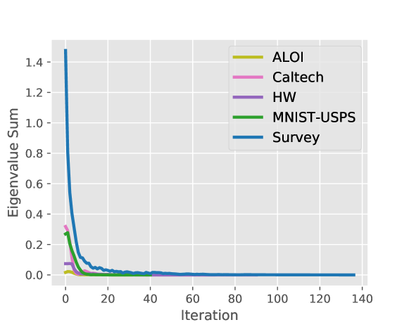
Figure 3: The sum of $k$ smallest eigenvalues on $k$-partition clustering over five datasets.

Table I reveals the promising ability of ANN in analyzing multi-view data. We can observe that ANN outperforms all state-of-the-art on ALOI and Caltech. In particular, ANN improves in NMI, Purity, and F-Score by 0.063, 0.115, 0.115 on ALOI and 0.042, 0.118, 0.017 on Caltech. ANN also achieves the state-of-the-art performance on HW and MNIST-USP. Although GMC achieves the best performance on MNIST-USP, it shows bad robustness on other datasets, e.g., from the aspect of NMI on ALOI and Caltech, GMC only obtains 0.794 and 0.764 on ALOI while ANN achieves 0.980 and 0.829, respectively. Table II shows the methods’ performance on the multi-layer Survey dataset. Most of the multi-view algorithms, e.g., GMC and BMVC, cannot work well with the two-layer view structure of Survey that their NMI scores are lower than SC’s. Both ANN and ANNLD achieve excellent performance on Survey. We can observe that ANN without learnable data space can still achieve the state-of-the-art performance and ANNLD improves NMI and F-Score by 0.077 and 0.073 than Co-training, demonstrating the effectiveness of proposed agglomerative analysis in utilizing complex view structure. ANNLD obtains better performance on all the matrices than ANN, which shows the effectiveness of learnable data space. Note that although SC achieves better Recall performance than ANN and ANNLD, it does not mean that SC is superior to the proposed methods, because SC’s best performance is achieved by partitioning almost all samples to a single cluster.

In all, our proposed ANN and ANNLD consistently show the best robustness and performance over five diverse datasets. The agglomerative consensus analysis and learnable data space can enhance the methods’ ability to analyze standard multi-view datasets, as well as handling the multi-layer structured dataset effectively.

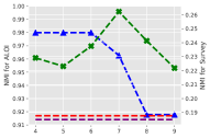
(a) Exponent of $\lambda_{max}$

(b) Parameter-$lr$

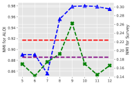
(c) neighbor Number

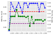
(d) Parameter-$\mathcal{P}$

Figure 4: Our model’s NMI under varying hyper-parameters on ALOI and Survey.

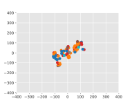
(a) $t=0$ (Raw Data)

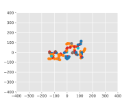
(b) $t=10$

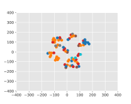
(c) $t=30$

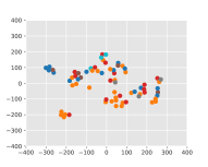
(d) $t=84$ (Converged)

Figure 5: Visualization of Two-layered Survey data embedding space.

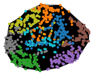
(a) $t=0$ (Raw Graph)

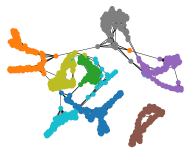
(b) $t=10$

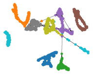
(c) $t=25$

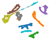
(d) $t=36$ (Converged)

Figure 6: Visualization of ALOI connection graphs.

V-C Hyper-parameter and Convergence Analysis

We take ALOI and Survey to study the influence of hyper-parameters on ANN and ANNLD, respectively. We set the learning rate, $lr$, around its optimal values: 0.05 and 0.1, separately; the results (Fig. 4) show our model is robust in terms of achieving the best performance under most hyper-parameter configurations when compared with the best performance of state-of-the-art (denoted by the red and purple horizontal lines). Our networks are predominantly influenced by the number of neighbors, especially on Survey data. In particular, ANNLD may perform poorly if the neighbor number is excessively small or large.

Our convergence analysis of the Constrained Laplacian rank of ANN (Fig. 3) shows that ANN can converge quickly by decreasing the eigenvalue sum to around zero within 20 iterations on all the five datasets, which contain varying quantities from 71 to 4,000.

V-D Embedding Visualization of Hidden Data Space

The embedding graphs indicate the effectiveness of data space projection of ANNLD in Fig. 5. We apply $K$-Means to transform input data into a 6-dimension distance vector and exhibit the T-distributed Stochastic Neighbor Embedding (t-SNE) with 2-component and 8-perplexity. We can observe that the raw data space has limited capability of distinguishing data that contain overlapping points. After iterations, the embedding points turns to be better distributed and distinct. It is easy to distinguish the purple and green points from other points when the algorithm converges.

V-E Visualization of Connection Graphs

We take ALOI as an example to illustrate how the optimization changes connection graphs in Fig. 6. We can observe that the raw graph only contains one cluster, and many connections exist between different classes. After iterations, ANN could effectively delete most redundant edges within several iterations. When the optimization converges, ANN can obtain a connection graph with exactly eight connected components. Each component could represent one cluster so that the connected component results could be directly used as the clustering results. Only a few points are clustered into the wrong connected components.

VI Conclusion

We propose agglomerative consensus analysis for multi-view clustering. To this end, we present an extensible Agglomerative Neural Network (ANN) and conduct comprehensive experiments over four public datasets. We further propose ANN with Learnable Data space (ANNLD) via an extra data projection to improve the raw data distribution under complex view structures with more than two layers. We have agglomerated converted subviews using only the weighted relationship, which has proven to achieve excellent performance. In light of the flexibility of ANN, we plan to extend ANN with more agglomerative relationships, e.g., convolutional networks, to solve general multi-view problems in more scenarios in the future. Besides, we will extend the proposed methods with matrix factorization to accelerate multi-view clustering.

References

- [1] F. Nie, X. Wang, M. I. Jordan, and H. Huang, “The constrained laplacian rank algorithm for graph-based clustering,” in Thirtieth AAAI Conference on Artificial Intelligence, 2016.
- [2] R. Vidal, “Subspace clustering,” IEEE Signal Processing Magazine, vol. 28, no. 2, pp. 52–68, 2011.
- [3] H.-P. Kriegel, P. Kröger, J. Sander, and A. Zimek, “Density-based clustering,” Wiley Interdisciplinary Reviews: Data Mining and Knowledge Discovery, vol. 1, no. 3, pp. 231–240, 2011.
- [4] M. Kleindessner, S. Samadi, P. Awasthi, and J. Morgenstern, “Guarantees for spectral clustering with fairness constraints,” arXiv preprint arXiv:1901.08668, 2019.
- [5] O. Oyelade, O. Oladipupo, and I. Obagbuwa, “Application of k means clustering algorithm for prediction of students academic performance,” arXiv preprint arXiv:1002.2425, 2010.
- [6] X. Peng, J. Feng, J. T. Zhou, Y. Lei, and S. Yan, “Deep subspace clustering,” IEEE Transactions on Neural Networks and Learning Systems, 2020.
- [7] E. Ergul, N. Arica, N. Ahuja, and S. Erturk, “Clustering through hybrid network architecture with support vectors,” IEEE transactions on neural networks and learning systems, vol. 28, no. 6, pp. 1373–1385, 2016.
- [8] F. Nie, G. Cai, and X. Li, “Multi-view clustering and semi-supervised classification with adaptive neighbours,” in Thirty-First AAAI Conference on Artificial Intelligence, 2017.
- [9] Z. Fu, W. Hu, and T. Tan, “Similarity based vehicle trajectory clustering and anomaly detection,” in IEEE International Conference on Image Processing 2005, vol. 2. IEEE, 2005, pp. II–602.
- [10] Y. Li, F. Nie, H. Huang, and J. Huang, “Large-scale multi-view spectral clustering via bipartite graph,” in Twenty-Ninth AAAI Conference on Artificial Intelligence, 2015.
- [11] X. Peng, Z. Huang, J. Lv, H. Zhu, and J. T. Zhou, “Comic: Multi-view clustering without parameter selection,” in International Conference on Machine Learning, 2019, pp. 5092–5101.
- [12] A. Kumar, P. Rai, and H. Daume, “Co-regularized multi-view spectral clustering,” in Advances in neural information processing systems, 2011, pp. 1413–1421.
- [13] A. Kumar and H. Daumé, “A co-training approach for multi-view spectral clustering,” in Proceedings of the 28th International Conference on Machine Learning (ICML-11), 2011, pp. 393–400.
- [14] G. Ma, L. He, C.-T. Lu, W. Shao, P. S. Yu, A. D. Leow, and A. B. Ragin, “Multi-view clustering with graph embedding for connectome analysis,” in Proceedings of the 2017 ACM on Conference on Information and Knowledge Management. ACM, 2017, pp. 127–136.
- [15] L. Zhao, Z. Chen, Y. Yang, Z. J. Wang, and V. C. Leung, “Incomplete multi-view clustering via deep semantic mapping,” Neurocomputing, vol. 275, pp. 1053–1062, 2018.
- [16] Z. Kun, Z. Changqing, G. Junpeng, and W. Junsheng, “Graph learning for multiview clustering.” IEEE transactions on cybernetics, vol. 48, no. 10, p. 2887, 2018.
- [17] X. He, L. Li, D. Roqueiro, and K. Borgwardt, “Multi-view spectral clustering on conflicting views,” in Joint European Conference on Machine Learning and Knowledge Discovery in Databases. Springer, 2017, pp. 826–842.
- [18] F. Pedregosa, G. Varoquaux, A. Gramfort, V. Michel, B. Thirion, O. Grisel, M. Blondel, P. Prettenhofer, R. Weiss, V. Dubourg, J. Vanderplas, A. Passos, D. Cournapeau, M. Brucher, M. Perrot, and E. Duchesnay, “Scikit-learn: Machine learning in Python,” Journal of Machine Learning Research, vol. 12, pp. 2825–2830, 2011.
- [19] Z. Zhang, L. Liu, F. Shen, H. T. Shen, and L. Shao, “Binary multi-view clustering,” IEEE transactions on pattern analysis and machine intelligence, vol. 41, no. 7, pp. 1774–1782, 2018.
- [20] F. Nie, J. Li, X. Li et al., “Self-weighted multiview clustering with multiple graphs.” in IJCAI, 2017, pp. 2564–2570.
- [21] H. Wang, Y. Yang, and B. Liu, “Gmc: Graph-based multi-view clustering,” IEEE Transactions on Knowledge and Data Engineering, 2019.
- [22] C. Zhang, H. Fu, S. Liu, G. Liu, and X. Cao, “Low-rank tensor constrained multiview subspace clustering,” in Proceedings of the IEEE international conference on computer vision, 2015, pp. 1582–1590.
- [23] S. Zhou, X. Liu, M. Li, E. Zhu, L. Liu, C. Zhang, and J. Yin, “Multiple kernel clustering with neighbor-kernel subspace segmentation,” IEEE transactions on neural networks and learning systems, 2019.
- [24] G. Andrew, R. Arora, J. Bilmes, and K. Livescu, “Deep canonical correlation analysis,” in International conference on machine learning, 2013, pp. 1247–1255.
- [25] W. Wang, R. Arora, K. Livescu, and J. Bilmes, “On deep multi-view representation learning,” in International Conference on Machine Learning, 2015, pp. 1083–1092.
- [26] S. Wei, J. Wang, G. Yu, X. Zhang et al., “Multi-view multiple clusterings using deep matrix factorization,” arXiv preprint arXiv:1911.11396, 2019.
- [27] J. Wu, Z. Lin, and H. Zha, “Essential tensor learning for multi-view spectral clustering,” IEEE Transactions on Image Processing, vol. 28, no. 12, pp. 5910–5922, 2019.
- [28] C. Zhang, H. Fu, Q. Hu, X. Cao, Y. Xie, D. Tao, and D. Xu, “Generalized latent multi-view subspace clustering,” IEEE transactions on pattern analysis and machine intelligence, vol. 42, no. 1, pp. 86–99, 2018.
- [29] Z. Huang, J. T. Zhou, X. Peng, C. Zhang, H. Zhu, and J. Lv, “Multi-view spectral clustering network,” in Proceedings of the Twenty-Eighth International Joint Conference on Artificial Intelligence. International Joint Conferences on Artificial Intelligence Organization, 2019, pp. 2563–2569.
- [30] U. Von Luxburg, “A tutorial on spectral clustering,” Statistics and computing, vol. 17, no. 4, pp. 395–416, 2007.
- [31] H. Lütkepohl, Handbook of matrices. Wiley Chichester, 1996, vol. 1.
- [32] U. Baruah and S. M. Hazarika, “A dataset of online handwritten assamese characters.” Journal of Information Processing Systems, vol. 11, no. 3, 2015.
- [33] Y. LeCun, L. Bottou, Y. Bengio, and P. Haffner, “Gradient-based learning applied to document recognition,” Proceedings of the IEEE, vol. 86, no. 11, pp. 2278–2324, 1998.
- [34] A. Demiriz, K. P. Bennett, and J. Shawe-Taylor, “Linear programming boosting via column generation,” Machine Learning, vol. 46, no. 1-3, pp. 225–254, 2002.
- [35] J.-M. Geusebroek, G. J. Burghouts, and A. W. Smeulders, “The amsterdam library of object images,” International Journal of Computer Vision, vol. 61, no. 1, pp. 103–112, 2005.
- [36] L. Fei-Fei, R. Fergus, and P. Perona, “Learning generative visual models from few training examples: An incremental bayesian approach tested on 101 object categories,” in 2004 conference on computer vision and pattern recognition workshop. IEEE, 2004, pp. 178–178.
- [37] S. R. Fanello, N. Noceti, G. Metta, and F. Odone, “Dictionary based pooling for object categorization,” in 2014 International Conference on Computer Vision Theory and Applications (VISAPP), vol. 2. IEEE, 2014, pp. 269–274.
- [38] P. Hartmann and V. Apaolaza-Ibáñez, “Consumer attitude and purchase intention toward green energy brands: The roles of psychological benefits and environmental concern,” Journal of business Research, vol. 65, no. 9, pp. 1254–1263, 2012.
- [39] C. A. Mandrik and Y. Bao, “Exploring the concept and measurement of general risk aversion,” ACR North American Advances, 2005.