Observational Learning with Fake Agents

Abstract

It is common in online markets for agents to learn from other’s actions. Such observational learning can lead to herding or information cascades in which agents eventually “follow the crowd”. Models for such cascades have been well studied for Bayes-rational agents that choose pay-off optimal actions. In this paper, we additionally consider the presence of fake agents that seek to influence other agents into taking one particular action. To that end, these agents take a fixed action in order to influence the subsequent agents towards their preferred action. We characterize how the fraction of such fake agents impacts behavior of the remaining agents and show that in certain scenarios, an increase in the fraction of fake agents in fact reduces the chances of their preferred outcome.

I Introduction

Consider a new item that is up for sale in a recommendation-based market where agents arrive sequentially and decide whether to buy the item, with their choice serving as a recommendation for later agents. Every agent makes a pay-off optimal decision based on his own prior knowledge of the item’s quality/utility and by observing the choices of his predecessors. An informational cascade or herding occurs when it is optimal for an agent to ignore his own private signal and follow the actions of the past agents. Subsequent agents follow suit and from the onset of a cascade, the agents’ actions do not reveal any information conveyed to them by their private signals. Thus the phenomenon of cascading could prevent the agents from learning the socially optimal (right) choice, i.e. the agents could herd to a wrong cascade.

Cascades were first studied in [1, 2, 3] as a Bayesian learning model in which a homogeneous sequence of rational agents take pay-off optimal actions. In this paper, in addition to rational agents, we introduce randomly arriving fake agents that always take (or fake) a fixed action, regardless of their pay-off, in order to influence the outcome of a cascade. For example, this could model a setting where a poor quality item is posted for sale on a website that records buyers’ decisions, and fake agents intentionally buy (or appear to buy) this item to make it seem worth buying to future buyers. The model could also represent a setting where rational actions are manipulated or where fake actions are inserted into a recommendation system. The objective is to study the impact of varying the amount of these fake agents on the probability of their preferred cascade. Our main result shows a counter-intuitive phenomenon: the probability with which this preferred cascade occurs is not monotonically increasing in the fraction of fake agents, $\epsilon$. In fact, in some cases the presence of fake agents can reduce the chance of their preferred cascade.

As in [1, 2, 3], we consider a setting in which all agents can observe all prior actions (although in our case, each action could be either rational or fake). Many other variations of this basic model have been studied such as [4], where observations depend on an underlying network structure and [5], where agents are allowed to select their observations at a cost.

Closer to our work is the model in [6], which assumes that the recording of actions for subsequent agents is subject to an error that is unbiased towards each of the possible actions. In our setting, an action being either fake or rational depending on the agent-type could equivalently be perceived as an error while recording a rational action (as in [6]); except that in our case, the error is biased only towards a preferred action.

There is also a body of work that considers agents similar to our fake agents, who only take a single action regardless of the true state. This includes the crazy agents considered in [7], stubborn agents in [8] and zealots in [9]. While [7] relaxes the assumption of binary signals, it does not consider how changing the fraction of crazy agents affects the cascade probability, which is the main focus of our work. In [8] a non-Bayesian model for learning was considered instead of the Bayesian model considered here. Other related cascade models are investigated in [10, 11, 12, 13, 14, 15, 16, 17].

The paper is organized as follows. We describe our model in Section II. We analyze this model and identify the resulting cascade properties in Section III. In Section IV, we present our Markov process formulation and in Section V, we consider the limiting scenario where the proportion of fake agents approaches unity. Section VI characterizes the asymptotic welfare of rational agents. We conclude in Section VII.

II Model

We consider a model similar to [1] in which there is a countable sequence of agents, indexed $i=1,2,\ldots$ where the index represents both the time and the order of actions. Each agent $i$ takes an action $A_{i}$ of either buying $(Y)$ or not buying $(N)$ a new item that has a true value $(V)$ which could either be good $(G)$ or bad $(B)$. For simplicity, both possibilities of $V$ are assumed to be equally likely. The agents are Bayes-rational utility maximizers where the pay-off received by each agent $i$, denoted by $\pi_{i}$, depends on its action $A_{i}$ and the true value $V$ as follows. If the agent chooses $N$, his payoff is $0$. Whereas, if the agent chooses $Y$, he incurs a cost of $C=1/2$ for buying the item, and gains the amount $0$ if $V=B$ and $1$ if $V=G$. The buyer’s net pay-off is then the gain minus the cost of buying the item. Observe that when $V$ is equiprobable, the ex ante expected pay-off is $0$ for either of the actions. Thus, at the start, an agent is indifferent to the two actions.

To incorporate agents’ private beliefs about the new item, every agent $i$ receives a private signal $S_{i}\in\{H\,\text{(high)},L\,\text{(low)}\}$. This signal, as shown in Figure 1$(a)$, partially reveals the information about the true value of the item through a binary symmetric channel (BSC) with crossover probability $1-p$, where $\nicefrac{{1}}{{2}}<p<1$. Each agent $i$ takes a rational action $A_{i}$ that depends on his private signal $S_{i}$ and the past observations $\{O_{1},O_{2},\ldots,O_{i-1}\}$ of actions $\{A_{1},A_{2},\ldots,A_{i-1}\}$. Next, we modify the information structure in [1] by assuming that at each time instant, an agent could either be fake with probability (w.p.) $\epsilon\in[0,1)$ or ordinary w.p. $1-\epsilon$. An ordinary agent $i$ honestly reports his action, i.e. $O_{i}=A_{i}$. On the contrary, a fake agent always reports a $Y$, reflecting his intention of influencing the successors into buying the new item, regardless of its true value. This implies that at any time $i$, with probability $1-\epsilon$, the reported action $O_{i}$ satisfies $O_{i}=A_{i}$ and with probability $\epsilon$, $O_{i}=Y$. Refer to Figure 1$(b)$.

An equivalent model is where a fake agent always takes an action $Y$, while $O_{i}=A_{i}$ for all agents. This yields the same information structure as the model above. However we chose the former model mainly to simplify our notation.

(a)

(b)

Figure 1: $(a)$ The BSC through which agents receive private signals. $(b)$ The channel through which agents’ actions are corrupted.

III Optimal decision and cascades

For the $n^{\text{th}}$ agent, let the history of past observations be denoted by $\mathcal{H}_{n-1}=\{O_{1},O_{2},\ldots,O_{n-1}\}$. As the first agent does not have any observation history, he always follows his private signal i.e., he buys if and only if the signal is $H$. For the second agent onwards, the Bayes’ optimal action for every agent $n$, $A_{n}$ is chosen according to the hypothesis ($V=G$ or $B$) that has the higher posterior probability given the information set $\mathbb{I}_{n}=\{S_{n},\mathcal{H}_{n-1}\}$. Let $\gamma_{n}(S_{n},\mathcal{H}_{n-1})\triangleq\mathbb{P}(G|S_{n},\mathcal{H}_{n-1})$ denote the posterior probability for the item being good, $V=G$ . Then the Bayes’ optimal decision rule is:

$$A_{n}=\begin{cases}Y,\quad&\text{if}\;\;\gamma_{n}>1/2,\\ N,\quad&\text{if}\;\;\gamma_{n}<1/2,\\ \text{follows}\;\;S_{n},\quad&\text{if}\;\;\gamma_{n}=1/2.\end{cases}$$ (1)

Note that when $\gamma_{n}=1/2$, an agent is indifferent between the actions. Similar to [6], our decision rule in this case follows the private signal $S_{n}$, unlike [1] where they employ random tie-breaking.

Definition 1

An information cascade is said to occur when an agent’s decision becomes independent of his private signal

It follows from (1) that, agent $n$ cascades to a $Y$ $(N)$ if and only if $\gamma_{n}>1/2$ $(<1/2)$ for all $S_{n}\in\{H,L\}$. The other case being $\gamma_{n}>1/2$ for $S_{n}=H$ and less than $1/2$ for $S_{n}=L$; in which case, agent $n$ follows $S_{n}$. A more intuitive way to express this condition is by using the information contained in the history $\mathcal{H}_{n-1}$ observed by agent $n$ in the form of the likelihood ratio $l_{n-1}(\mathcal{H}_{n-1})\triangleq\mathbb{P}(\mathcal{H}_{n-1}|B)/\mathbb{P}(\mathcal{H}_{n-1}|G)$ as follows [7].

Lemma 1

Agent $n$ cascades to a $Y\,(N)$ if and only if $l_{n-1}<\frac{1-p}{p}$ $\big{(}l_{n-1}>\frac{p}{1-p}\big{)}$ and otherwise follows its private signal $S_{n}$.

This lemma follows by expressing $\gamma_{n}$ in terms of $l_{n-1}$ using Bayes’ law, and then using the condition on $\gamma_{n}$ for a $Y\,(N)$ cascade. If agent $n$ cascades, then the observation $O_{n}$ does not provide any additional information about the true value $V$ to the successors than what is contained in $\mathcal{H}_{n-1}$. As a result, $l_{n+i}=l_{n-1}$ for all $i=0,1,2,\ldots$ and hence they remain in the cascade, which leads us to the following property, also exhibited by prior models [1, 2, 3, 6].

Property 1

Once a cascade occurs, it lasts forever.

On the other hand, if agent $n$ does not cascade, then Property 1 and Lemma 1 imply that all the agents until and including $n$ follow their own private signals ignoring the observations of their predecessors. Mutual independence between the private signals results in the likelihood ratio $l_{n}$ depending only on the number of $Y$’s (denoted by $n_{Y}$) and $N$’s (denoted by $n_{N}$) in the observation history $\mathcal{H}_{n}$. Specifically, $l_{n}=\left(\frac{1-p}{p}\right)^{h_{n}}$ where $h_{n}=\eta n_{Y}-n_{N}$ is the difference between the number of $Y$’s weighted by $\eta$ and the number of $N$’s. Here, the weight $\eta\triangleq\log(\frac{a}{1-b})/\log(\frac{p}{1-p})$, where for all $i=1,2,\ldots,n-1$,

$$a=\mathbb{P}(O_{i}=Y|V=G)\quad\text{and}\quad b=\mathbb{P}(O_{i}=N|V=B)$$

give the probabilities that the observations follow the true value $V$, given that these agents follow their own private signals. It can be shown from Figures 1$(a)$ and 1$(b)$ that in the above case, i.e., when $A_{i}$ follows $S_{i}$,

$$a=p+(1-p)\epsilon\;\;\text{and}\;\;b=p(1-\epsilon).$$

Thus, agents that have not yet entered a cascade satisfy the following property.

Property 2

Until a cascade occurs, each agent follows its private signal. Moreover, $h_{n}$ is a sufficient statistic of the information contained in the past observations.

Note that if $\epsilon=0$ (no fake agents) then $a=b=p$ and $\eta=1$, in which case $h_{n}$ is the same as in [6]. The expression for $h_{n}$ shows that, due to the presence of fake agents, the dependence of an agent’s decision on a $Y$ in his observation history reduces by a factor of $\eta$, whereas the dependence on a $N$ remains unaffected. This is to be expected because, unlike a $N$ which surely comes from an honest agent, a $Y$ incurs the possibility that the agent could be fake. Further, this reduced dependence on $Y$ is exacerbated with an increase in the possibility of fake agents, as $\eta$ reduces with an increase in $\epsilon$.

Using the expression for $l_{n}$ in Lemma 1, it follows that until a cascade occurs, $-1\leq h_{n}\leq 1$ for all such times $n$, and the update rule for $h_{n}$ is given by

$$h_{n}=\begin{cases}h_{n-1}+\eta\quad&\text{if}\;\;O_{n}=Y,\\ h_{n-1}-1\quad&\text{if}\;\;O_{n}=N.\end{cases}$$ (2)

Whereas, once $h_{n}>1$ ($<-1$), a $Y\,(N)$ cascade begins and $h_{n}$ stops updating (Property 1).

IV Markovian Analysis of Cascades

Let us, for the sake of discussion, consider the realization $V=B$ . Similar arguments hold when $V=G$ . It follows from the previous section that the process $\{h_{n}\}$ is a discrete-time Markov process taking values in $[-1,1]$ before getting absorbed into the left wall $(<-1)$ causing a $N$ cascade or the right wall $(>1)$ causing a $Y$ cascade. More specifically, equation (2) shows that, until a cascade occurs, $\{h_{n}\}$ is a random walk that shifts to the right by $\eta$ w.p. $\mathbb{P}(O_{n}=Y|B)=1-b$ or to the left by $1$ w.p. $\mathbb{P}(O_{n}=N|B)=b$. Note that the walk starts at state $0$ since the first agent has no observation history.

The random walk is depicted in Figure 2 where $p_{f}\triangleq\mathbb{P}(O_{n}=Y|V)$ denotes the probability of a $Y$ being observed. Depending on the item’s true value, $p_{f}=a$ for $V=G$ whereas $p_{f}=1-b$ for $V=B$. Note that in the special case where $\eta$ satisfies $1/\eta=r$ for some $r=1,2,\ldots$, the process $\{h_{n}\}$ is equivalent to a Markov Chain with finite state-space $\mathcal{A}=\{-r-1,-r,\ldots,-1,0,1,\ldots,r,r+1\}$ , and with $-r-1$ and $r+1$ being absorption states corresponding to $N$ and $Y$ cascades respectively. In this case, absorption probabilities can be obtained by solving a system of linear equations. In this paper, our main focus is on the more common case of non-integer values of $1/\eta$ resulting in $\{h_{n}\}$ taking possibly uncountable values in $[-1,1]$.

Figure 2: Transition diagram of the random walk.

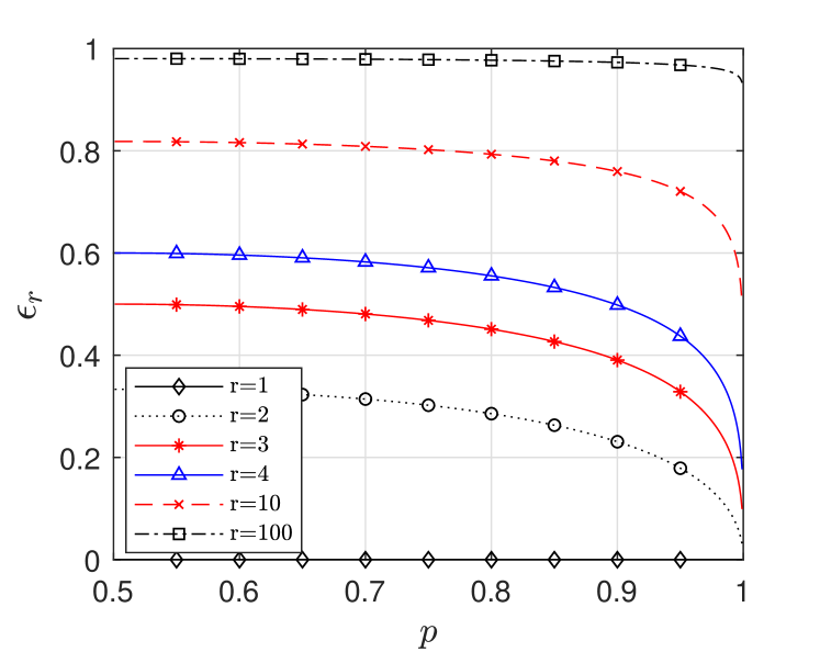
Figure 3: Thresholds $\epsilon_{r}$ for the indicated values of $r$ versus $p$.

IV-A Error thresholds

In the absence of fake agents $(\epsilon=0)$ as in [1], $\eta=1$ and so cascading to a $Y(N)$ cascade requires at least two consecutive $Y$’s ($N$’s). However, in the presence of fake agents, even a single $N$ after a $Y$ could trigger a $N$ cascade. On the other hand, as $\epsilon$ increases, a greater number of consecutive $Y$’s $(\geq 2)$ are required to cause a $Y$ cascade. This is characterized in the following lemma.

Lemma 2

Let $\alpha=p/(1-p)$. For $r=1,2,\ldots$ define the increasing sequence of thresholds $\{\epsilon_{r}\}_{r=1}^{\infty}$, where the $r^{\text{th}}$ threshold $\epsilon_{r}$ is given as:

$$\epsilon_{r}=\frac{\alpha-\alpha^{\frac{1}{r}}}{\alpha^{\frac{1}{r}+1}-1}.$$ (3)

Define $\mathcal{I}_{r}\triangleq[\epsilon_{r},\epsilon_{r+1})$ as the $r^{\text{th}}$ $\epsilon$–interval. Then for $\epsilon\in\mathcal{I}_{r}$, at least $r+1$ consecutive $Y$’s are necessary for a $Y$ cascade to begin.

The proof follows by noting that, given that if a cascade has not begun, when an $N$ is observed, then the rightmost position that the random walk can be in, is in state $0$. From here, at least $r+1$ consecutive $Y$’s would be needed only if $\eta\leq 1/r$, thereby giving the $r^{\text{th}}$ threshold $\epsilon_{r}$. It follows that $\epsilon\in\mathcal{I}_{r}$ implies $\frac{1}{r+1}<\eta\leq\frac{1}{r}$ .

Remark 1

For $\epsilon\in\mathcal{I}_{r}$, staring from state $0$, $r+1$ consecutive $Y$’s start a $Y$ cascade.

Moreover, given $\epsilon$, the integer $r$ such that $\epsilon\in\mathcal{I}_{r}$ can be readily obtained from Lemma 2 as $r=\left\lfloor 1/\eta\right\rfloor$. Here, recall that $\eta$ is a function of $\epsilon$.

Figure 3 shows the thresholds $\epsilon_{r}$ varying with $p$, for different values of $r$. For a fixed $\epsilon$, we see that as the signal quality ($p$) improves, more consecutive $Y$’s are required for a $Y$ cascade to begin. This is because, an increase in $p$ increases the information contained in a $Y$, but not as much as the corresponding increase in the information contained in a $N$. Further, note that as $\epsilon\rightarrow 1$, $r\rightarrow\infty$ which implies that infinitely many consecutive $Y$’s are required for a $Y$ cascade to begin. Equivalently, the information contained in a $Y$ observation becomes negligible. We further investigate learning in this asymptotic scenario in Section V.

IV-B $Y$ cascade probability

In this subsection, we will compute the probability of absorption of $\{h_{n}\}$ to a $Y$ cascade (right wall). The following iterative process depicted in Figure 4 describes all possible sequences that can lead to a $Y$ cascade. For the rest of the paper, we assume $\epsilon\in\mathcal{I}_{r}\smallsetminus\{\epsilon_{r}\}$ for some $r=1,2,\ldots$. We initialize Stage $1$ with $r_{1}=r+1$. Now, starting from state $0$, consider the sequences shown in Stage $1$ in Figure 4. The first sequence of $r_{1}$ consecutive $Y$’s, denoted by $Y^{r_{1}}$, clearly hits the right wall (Remark 1). The rest of the sequences, each of length $r_{1}+1$, are simply permutations of each other that contain only a single $N$. Two $N$’s or more are not possible without hitting the left wall. So each of these $r_{1}$ distinct sequences results in the same net right shift, which ends somewhere in the region $[0,\eta]$. From here, it would take either $r$ or $r+1$ consecutive $Y$’s to hit the right wall. Let this value be denoted by $r_{2}$. The sequences that would then be possible from this point onwards could again be enumerated exactly as in the first stage, except that $r_{2}$ now replaces $r_{1}$. This forms Stage $2$. Now, unless there are $r_{2}$ consecutive $Y$’s, the second stage would again end in the region $[0,\eta]$, and then the process continues to the next stage. Here, $r_{n}$ denotes the number of consecutive $Y$’s required to hit the right wall in the $n^{\text{th}}$ stage. Note that by considering $\epsilon\in\mathcal{I}_{r}\smallsetminus\{\epsilon_{r}\}$, we avoid the case of integer values of $1/\eta$ which could result in certain pathological sequences with non-zero probability, that are not enumerated in Figure 4.

Figure 4: An enumeration of all possible sequences that would lead to a $Y$ cascade.

Let $S_{n}$ denote the probability of hitting the right wall given that the sequence has not terminated before the $n^{\text{th}}$ stage. Thus, the following recursion holds:

$$S_{n}=p_{f}^{r_{n}}\big{[}1+r_{n}(1-p_{f})S_{n+1}\big{]},\;\;\text{for}\;n=1,2,\ldots$$ (4)

and the probability of a $Y$ cascade, denoted by $\mathbb{P}_{Y\text{-cas}}$ is:

$$\mathbb{P}_{Y\text{-cas}}(\epsilon)=S_{1},\quad\text{for}\;\;\epsilon\in\mathcal{I}_{r}\smallsetminus\{\epsilon_{r}\}.$$ (5)

Here, while $r_{1}=r+1$ for $\epsilon\in\mathcal{I}_{r}$, successive values of $r_{i}$ for $i=2,3,\ldots$ can be obtained from $r_{1}$ using the updates:

$$r_{n}=\begin{cases}\text{\scalebox{0.9}{$r$}},\quad&\text{if}\;\;\text{\scalebox{0.9}{$\sum_{i=1}^{n-1}(r_{i}\eta-1)+r\eta>1$}},\\ \text{\scalebox{0.9}{$r+1$}},\quad&\text{o.w.}\end{cases}$$ (6)

Since (4) is an infinite recursion, to compute $\mathbb{P}_{Y\text{-cas}}$ in practice, we truncate the process to a finite number of iterations $M$. To this end, we first assume that $S_{M+1}=1$. Next, we use (4) to successively compute $S_{k}$ while $k$ counts down from $M$ to $1$, performing a total of $M$ iterations. We denote the obtained value as $\mathbb{P}_{Y\text{-cas}}^{M}$ . We now state in the following theorem that $\mathbb{P}_{Y\text{-cas}}^{M}$ is in fact a tight upper bound to $\mathbb{P}_{Y\text{-cas}}$ as $M\rightarrow\infty$. Moreover, the difference $\mathbb{P}_{Y\text{-cas}}^{M}-\mathbb{P}_{Y\text{-cas}}$ decays to zero at least as fast as $\{0.5^{M}\}$, in the number of iterations $M$.

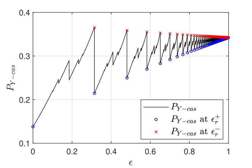
Figure 5: Probability of $Y$ cascade as a function of $\epsilon$ for $V=B$ and $p=0.7$.

Theorem 1

Let $\epsilon\in\mathcal{I}_{r}$ for some $r=1,2,\ldots$, with $p_{f}$ denoting the probability of a $Y$. Then, for any $M=1,2,\ldots$,

$$0\,\leq\;\mathbb{P}_{Y\text{-cas}}^{M}(\epsilon)-\mathbb{P}_{Y\text{-cas}}(\epsilon)\;\leq\,k^{M},$$

where $k\triangleq(r+1)(1-p_{f})p_{f}^{r}$ and for any $p\in(0.5,1)$ and $\epsilon\in[0,1)$, $k$ satisfies $0<k\leq 1/2$.

Proof:

Recall that $S_{M+1}=1$ while computing $\mathbb{P}_{Y\text{-cas}}^{M}$ , which implies that $\mathbb{P}_{Y\text{-cas}}^{M}$ is the net probability of: $(a)$ sequences that terminate in a $Y$ cascade by the $M^{\text{th}}$ stage and $(b)$ sequences that do not terminate by the $M^{\text{th}}$ stage. Thus, the difference: $\mathbb{P}_{Y\text{-cas}}^{M}-\mathbb{P}_{Y\text{-cas}}$ is upper-bounded by the probability of $(b)$. Accounting for all possible sequence combinations that persist through stages $1,2,\ldots,M$ yields the probability $k$. Next, for a fixed $p$ and for $\epsilon\in\mathcal{I}_{r}$, $k$ is maximized only if $\epsilon$ is such that $p_{f}=\frac{r}{1+r}$, which may not be satisfied for any $\epsilon$ in $\mathcal{I}_{r}$. Assuming $k$ is maximized, the maximal value of $k$ would be $\big{(}\frac{r}{1+r}\big{)}^{r}$. As this maximal value decreases in $r$, evaluating it at $r=1$ yields $k\leq 1/2$ for any $r$. ∎

Figure 5 shows a plot of $\mathbb{P}_{Y\text{-cas}}$ with respect to $\epsilon$, for the case $V=B$ with $p=0.7$. The plot uses $M=10$ which gives an error of less than $10^{-3}$. It can be seen that in the $r^{\text{th}}$ $\epsilon$–interval $\mathcal{I}_{r}$, $\mathbb{P}_{Y\text{-cas}}$ increases with $\epsilon$, but with infinitely many discontinuities (where $\mathbb{P}_{Y\text{-cas}}(\epsilon)$ decreases). Despite the discontinuities, $\mathbb{P}_{Y\text{-cas}}$ achieves the minimum and maximum values at the edge points of $\mathcal{I}_{r}$, i.e., $\epsilon_{r}^{+}$ and $\epsilon_{r+1}^{-}$, respectively. Further, note that the relatively larger drops in $\mathbb{P}_{Y\text{-cas}}(\epsilon)$ observed in Figure 5 (marked by $\times$ and $\circ$) occur exactly at the threshold points $\{\epsilon_{r}\}_{r=1}^{\infty}$. Here, counter to expectation, a slight increase in $\epsilon$ beyond $\epsilon_{r}$ causes a significant decrease in the probability of a $Y$ cascade.

We now quantify $\mathbb{P}_{Y\text{-cas}}$ as $\epsilon$ tends to each threshold point $\epsilon_{r}$. For this, we state the following lemma:

Lemma 3

For all $i\geq 2$, $r_{i}\rightarrow r$ as $\epsilon\rightarrow\epsilon_{r}$.

Proof:

We consider two cases: $\epsilon\rightarrow\epsilon_{r}^{+}$ and $\epsilon\rightarrow\epsilon_{r}^{-}$. The proof outline for the first case is as follows: assume $r_{j}=r$ for all $2\leq j\leq i-1$ and note that $r_{1}=r+1$ as $\epsilon_{r}^{+}\in\mathcal{I}_{r}$. Then it follows from (6) that $r_{i}=r$ only if $\eta>\big{(}r+\frac{1}{i}\big{)}^{-1}$. Now as $\epsilon\rightarrow\epsilon_{r}^{+}$, $\eta\rightarrow 1/r$ and hence the condition for $r_{i}=r$ is satisfied. Using this argument inductively shows that $r_{i}=r$ for all $i\geq 2$. The second case is proved similarly. ∎

It follows from Lemma 3 that as $\epsilon\rightarrow\epsilon_{r}$, the recursion in (4) results in the same infinite computation to obtain $S_{i}$ as for $S_{i+1}$, for all $i\geq 2$. Thus, all $S_{i}$ for $i\geq 2$ have the same value which satisfies: $S_{i}=p_{f}^{r}\big{[}1+r(1-p_{f})S_{i}\big{]}$ . Solving this equation for $i=2$ gives the value for $S_{2}$ which when used in equation (4) for $n=1$ yields $S_{1}$, i.e., $\mathbb{P}_{Y\text{-cas}}$. However, note that while solving equation (4), $r_{1}=r+1$ for $\epsilon=\epsilon_{r}^{+}$ whereas $r_{1}=r$ for $\epsilon=\epsilon_{r}^{-}$. This corresponds to the following two different values of $\mathbb{P}_{Y\text{-cas}}$ as $\epsilon\rightarrow\epsilon_{r}$:

$$\mathbb{P}_{Y\text{-cas}}(\epsilon_{r}^{+}) =\text{\scalebox{0.9}{$\displaystyle p_{f}^{r+1}\frac{1+(1-p_{f})p_{f}^{r}}{1-r(1-p_{f})p_{f}^{r}}$}},$$ (7)

$$\mathbb{P}_{Y\text{-cas}}(\epsilon_{r}^{-}) =\text{\scalebox{0.9}{$\displaystyle p_{f}^{r}\frac{1}{1-r(1-p_{f})p_{f}^{r}}$}}.$$ (8)

Hence, the fractional decrease in $\mathbb{P}_{Y\text{-cas}}$ that occurs abruptly at $\epsilon_{r}$, defined as $\delta_{r}=\big{[}\mathbb{P}_{Y\text{-cas}}(\epsilon_{r}^{-})-\mathbb{P}_{Y\text{-cas}}(\epsilon_{r}^{+})\big{]}/\mathbb{P}_{Y\text{-cas}}(\epsilon_{r}^{-})$ is:

$$\delta_{r}=(1-p_{f})\,(1-p_{f}^{r+1}).$$ (9)

It can be verified that as $r\rightarrow\infty$, $\delta_{r}\rightarrow 0$. This is depicted in Figure 5 where the sequences $\{\mathbb{P}_{Y\text{-cas}}(\epsilon_{r}^{-})\}$ and $\{\mathbb{P}_{Y\text{-cas}}(\epsilon_{r}^{+})\}$ , marked by $\times$ and $\circ$ respectively, converge to a limiting value as $r\rightarrow\infty$.

Property 3

If the possibility of fake agents in the history equals the $r^{th}$ $\epsilon$-threshold, $r=2,3,\ldots$, then a further increase in fake agents reduces the chances of a $Y$ cascade by a factor of $\delta_{r}$, rather than increasing it.

Next, we consider the cascade behaviour for low values of $\epsilon$ and state the following theorem.

Theorem 2

Given the private signal quality $p\in(0.5,1)$, and the item’s true value $V\in\{G,B\}$, there exists some $\underline{\epsilon}=f(V,p)>0$ such that

$$\mathbb{P}_{Y\text{-cas}}(\epsilon)<\mathbb{P}_{Y\text{-cas}}(0),\quad\forall\;\;\epsilon\in(0,\underline{\epsilon}).$$ (10)

From the point of view of the fake agents, the above theorem implies that if they occur with a probability of less than $\underline{\epsilon}$, then the effect that their presence has on the honest buyers is opposite to what they had intended. That is, they reduce the chances of a $Y$ cascade instead of increasing it. On the other hand, for honest buyers, if $V=B$, then they benefit from the presence of fake agents. Otherwise if $V=G$, then they are harmed by the presence of fake agents.

The proof for Theorem 2 follows by noting that as $\epsilon\rightarrow 0$, the limiting value of $\mathbb{P}_{Y\text{-cas}}$ can be obtained from (7) with $r=1$ and $p_{f}\rightarrow 1-p$ for $V=B$, whereas $p_{f}\rightarrow p$ for $V=G$, which gives

$$\text{\scalebox{0.95}{$\lim_{\epsilon\rightarrow 0}\mathbb{P}_{Y\text{-cas}}(\epsilon)=$}}\begin{cases}\text{\scalebox{0.9}{$\displaystyle(1-p)^{2}\frac{1+p(1-p)}{1-p(1-p)}$}},\quad&\text{for}\;\;V=B,\vspace{2mm}\\ \text{\scalebox{0.9}{$\displaystyle p^{2}\frac{1+p(1-p)}{1-p(1-p)}$}},\quad&\text{for}\;\;V=G.\end{cases}$$ (11)

However, in the absence of fake agents $(\epsilon=0)$ as in [1], $\eta=1$. It then follows from Figure 2 that $\{h_{n}\}$ has a finite state-space $\{-2,-1,0,1,2\}$, and a $Y$ $(N)$ cascade starts when $h_{n}=2$ $(-2)$. Here, solving for $\mathbb{P}_{Y\text{-cas}}$ gives

$$\mathbb{P}_{Y\text{-cas}}(0)=\begin{cases}p^{2}/\big{[}p^{2}+(1-p)^{2}\big{]},&\text{for}\;V=G,\\ (1-p)^{2}/\big{[}p^{2}+(1-p)^{2}\big{]},\;&\text{for}\;V=B.\end{cases}$$ (12)

By comparing the above expression with the one in (11) for the corresponding values of $V,$ it follows that

$$\lim_{\epsilon\rightarrow 0}\mathbb{P}_{Y\text{-cas}}(\epsilon)<\mathbb{P}_{Y\text{-cas}}(0),\quad\forall\;p\in(0.5,1),V\in\{G,B\}.$$

Thus, there exists some $\underline{\epsilon}>0$ such that (10) holds true.

V Learning in the limit as $\epsilon\rightarrow 1$

As the probability of an agent being fake tends to $1$, the information contained in a $Y$ observation becomes negligible. As a result, an agent would need to observe infinitely many consecutive $Y$’s in his history for him to be convinced of starting a $Y$ cascade. Hence, one would expect that if $V=G$, learning would never occur, whereas if $V=B$, then learning would always occur. However, recall that as $\epsilon\rightarrow 1$, the occurrence of $Y$’s becomes increasingly frequent, i.e. $p_{f}\rightarrow 1$; for both $V=B$ and $G$. This motivates studying $\mathbb{P}_{Y\text{-cas}}$ in this limiting scenario. First, recall that in the process of enumerating all sequences leading to a $Y$ cascade, for $\epsilon\in\mathcal{I}_{r}$, in each stage $i\geq 2$, $r_{i}$ is either $r$ or $r+1$. However, $\epsilon\rightarrow 1$ implies $r\rightarrow\infty$, in which case $r\approx r+1$. As a result, the expressions obtained in (7) and (8) yield the same limiting value for $\mathbb{P}_{Y\text{-cas}}$ as $\epsilon_{r}\rightarrow 1$, i.e., $r\rightarrow\infty$. In particular,

$$\lim_{\epsilon\rightarrow 1}\mathbb{P}_{Y\text{-cas}}(\epsilon)=\lim_{r\rightarrow\infty}\mathbb{P}_{Y\text{-cas}}(\epsilon_{r}^{+})\overset{(a)}{=}\lim_{r\rightarrow\infty}\mathbb{P}_{Y\text{-cas}}(\epsilon_{r}^{-}),$$

where Step $(a)$ can be proved by recalling that $\delta_{r}\rightarrow 0$ as $r\rightarrow\infty$. Further, the limiting probability of a $Y$ cascade, in terms of $\alpha=p/(1-p)$, is given by (refer to References for proof):

$$\lim_{\epsilon\rightarrow 1}\mathbb{P}_{Y\text{-cas}}(\epsilon) =\lim_{r\rightarrow\infty}\text{\scalebox{0.9}{$\displaystyle p_{f}^{r}\frac{1}{1-r(1-p_{f})p_{f}^{r}}=\frac{1}{e^{t}-t}$}};$$ (13)

where $t=\frac{1}{\alpha-1}\log\alpha$ for $V=G$ , and $t=\frac{\alpha}{\alpha-1}\log\alpha$ for $V=B$ .

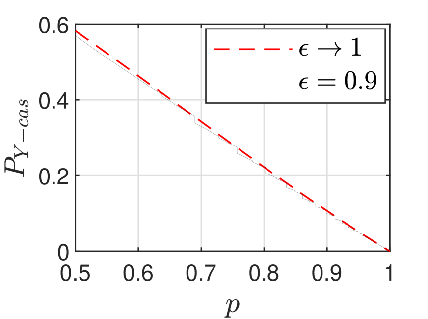
(a) $V=B$

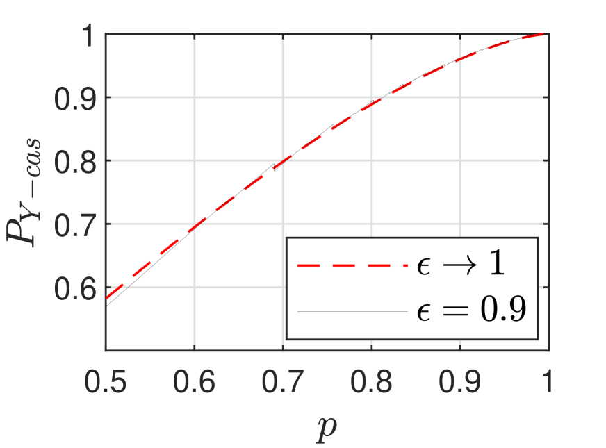
(b) $V=G$

Figure 6: Probability of $Y$ cascade versus private signal quality for the indicated values of $\epsilon$.

Figure 6 illustrates (13) and the corresponding probability when $\epsilon=0.9$ as a function of the signal quality. For both $V=B$ and $V=G$, a better signal quality leads to improved learning even when fake agents have overwhelmed the ordinary agents. Also note that for $V=B$, for a weak signal quality, the incorrect cascade is more likely than the correct one (while for $V=G$ this is never true).

VI Asymptotic welfare for ordinary agents

In this section, we analyze the expected pay-off or welfare of an ordinary (rational) agent $n$, $\mathbb{E}[\pi_{n}]$ as $n\rightarrow\infty$. Recall from Section II that $\pi_{n}=0$ if $A_{n}=N$ whereas $\pi_{n}=1/2$ or $-1/2$ if $A_{n}=Y$ depending on whether $V=G$ or $B$, respectively. Thus, agent $n$’s welfare is given by:

$$\mathbb{E}[\pi_{n}] =\mathbb{P}(A_{n}=Y|V=G)\frac{1}{4}-\mathbb{P}(A_{n}=Y|V=B)\frac{1}{4}.$$ (14)

Next, by taking the limit as $n\rightarrow\infty$ of (14), the asymptotic welfare $\underset{n\rightarrow\infty}{\lim}E[\pi_{n}(\epsilon)]$ denoted by $\Pi(\epsilon)$ is given by:

$$\Pi(\epsilon) =\frac{1}{4}\left[\mathbb{P}_{Y\text{-cas}}^{G}(\epsilon)-\mathbb{P}_{Y\text{-cas}}^{B}(\epsilon)\right]\overset{(b)}{=}\frac{1}{4}\big{(}1-2\mathbb{P}_{\text{wrong-cas}}(\epsilon)\big{)}.$$ (15)

In Step $(b)$, $\mathbb{P}_{\text{wrong-cas}}:=\left[\mathbb{P}_{N\text{-cas}}^{G}+\mathbb{P}_{Y\text{-cas}}^{B}\right]/2$ refers to the unconditional probability of a wrong cascade, i.e., the probability that a $N$ cascade occurs and $V=G$ or a $Y$ cascade occurs and $V=B$. The relation between $\mathbb{P}_{\text{wrong-cas}}(\epsilon)$ and $\Pi(\epsilon)$ presented by equation (15) substantiates the notion that a lower probability of wrong cascade results in higher asymptotic welfare. The probability $P_{Y\text{-cas}}^{V}(\epsilon)$ for $V\in\{G,B\}$ can be computed using the recursive method described in Section IV-B by equations (4) and (5). Then, substituting these obtained values in equation (15) yields the value for $\Pi(\epsilon)$. Figure 7 shows a plot of $\Pi(\epsilon)$ with respect to $\epsilon\in(0,1)$, for $p=0.7$ and compares it with the constant level of $\Pi(0)$ which refers to the asymptotic welfare in the absence of fake agents. We substitute (12) in (15) to obtain $\Pi(0)$, which gives

$$\Pi(0)=(1/4)(2p-1)/\big{[}\mspace{2.0mu}p^{2}+(1-p)^{2}\mspace{2.0mu}\big{]}.$$ (16)

It can be observed in Figure 7 that for $p=0.7$, $\Pi(\epsilon)<\Pi(0)$ for all $\epsilon\in(0,1)$. We find this ordering to be consistent over all values in the range of $p$.

Remark 2

For any private signal quality $p$, we observe that the presence of fake agents in any amount worsens the asymptotic welfare.

Further, note that the relatively larger jumps in $\Pi(\epsilon)$ observed in Figure 7 (marked by $\times$ and $\circ$) occur exactly at the threshold points $\{\epsilon_{r}\}_{r=2}^{\infty}$. Here, counter to expectation, a slight increase in $\epsilon$ beyond $\epsilon_{r}$ causes an abrupt and significant increase in the asymptotic welfare. Therefore increasing $\epsilon$ over the $r^{th}$ $\epsilon$-threshold is not only counter-productive for the fake agents but it also leads to a higher asymptotic welfare for the ordinary agents.

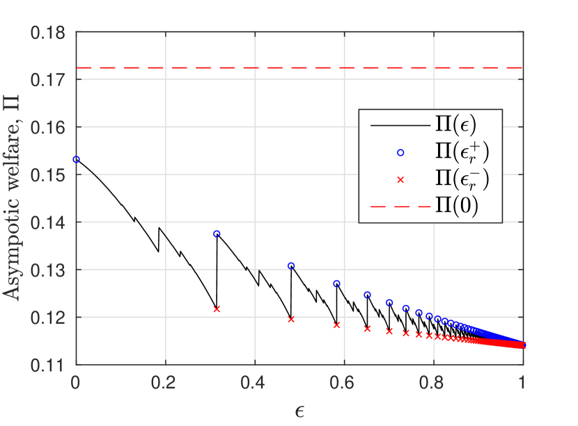
Figure 7: Asymptotic welfare as a function of $\epsilon$ for $p=0.7$.

VII Conclusions and future work

We studied the effect of randomly arriving fake agents that seek to influence the outcome of an information cascade. We focussed on the impact of varying the amount of fake agents on the probability of their preferred cascade and identified scenarios where the presence of fake agents reduces the chances of their preferred cascade. In particular, the chances of the preferred cascade decrease abruptly as the fraction of agents increase beyond specific thresholds. We quantified the correct cascade probability as a function of the private signal quality in the asymptotic regime where the fraction of fake agents approaches unity. We observed that the presence of fake agents in any amount worsens the asymptotic welfare. Studying the effects of multiple types of fake agents and non-Bayesian rationality are possible directions for future work.

Proof for equation (13)

Proof:

First, we first obtain the limitng value for the term $p_{f}^{r}$ as $r\rightarrow\infty$. For this, recall that as $r=\left\lfloor 1/\eta\right\rfloor$, we have $p_{f}^{1/\eta}\leq p_{f}^{r}<p_{f}^{1/\eta-1}$. Since the upper and lower bounds converge to the same limit, it implies that

$$\underset{r\rightarrow\infty}{\lim}p_{f}^{r}=\underset{\epsilon\rightarrow 1}{\lim}p_{f}^{1/\eta}.$$ (17)

Further, given that $\eta\triangleq\log(\frac{a}{1-b})/\log(\frac{p}{1-p})$, the numerator of $\eta$ can be bounded using the inequality: $1-x^{-1}\leq\log(x)\leq x-1$, which holds for all $x>0$. As a result, $\eta$ can be bounded as:

$$\frac{(2p-1)(1-\epsilon)}{\big{(}p+(1-p)\epsilon\big{)}\log\alpha}\leq\eta\leq\frac{(2p-1)(1-\epsilon)}{\big{(}1-p(1-\epsilon)\big{)}\log\alpha}.$$ (18)

This in turn extends to the following bounds on $p_{f}^{1/\eta}$,

$$p_{f}^{\frac{1}{1-p_{f}}at}\leq p_{f}^{1/\eta}\leq p_{f}^{\frac{1}{1-p_{f}}(1-b)t},$$ (19)

where $t=\frac{1}{\alpha-1}\log\alpha$ for $V=G$ , and $t=\frac{\alpha}{\alpha-1}\log\alpha$ for $V=B$ . Now, as both $a$ and $1-b$ tend to $1$ as $\epsilon\rightarrow 1$; both the upper and the lower bounds presented in (19) achieve the same limit. Hence,

$$\underset{r\rightarrow\infty}{\lim}p_{f}^{r}\overset{\eqref{p_f^r_limit}}{=}\underset{\epsilon\rightarrow 1}{\lim}p_{f}^{1/\eta}=\left(\underset{\epsilon\rightarrow 1}{\lim}p_{f}^{\frac{1}{1-p_{f}}}\right)^{t}\overset{(a)}{=}e^{-t},$$ (20)

where Step $(a)$ follows by reducing the limit term such that it maps to the identity: $\underset{x\rightarrow 0^{+}}{\lim}(1-x)^{\frac{1}{x}}=1/e$.

Secondly, we obtain the limitng value for the term $r(1-p_{f})$ which equals the limit for $(1-p_{f})/\eta$ because $r=\left\lfloor 1/\eta\right\rfloor$. Now, inequality (18) leads to the following bounds on $(1-p_{f})/\eta$:

$$\frac{(1-b)(1-p_{f})}{(2p-1)(1-\epsilon)}\log\alpha\leq\frac{1-p_{f}}{\eta}\leq\frac{a(1-p_{f})}{(2p-1)(1-\epsilon)}\log\alpha.$$

But as both $a$ and $1-b$ tend to $1$ as $\epsilon\rightarrow 1$; both the upper and the lower bounds presented above achieve the same limit. Hence,

$$\underset{\epsilon\rightarrow 1}{\lim}\;r(1-p_{f})=\underset{\epsilon\rightarrow 1}{\lim}\frac{1-p_{f}}{\eta}=\underset{\epsilon\rightarrow 1}{\lim}\frac{(1-p_{f})\log\alpha}{(2p-1)(1-\epsilon)}=t,$$ (21)

where $t$ has been defined for $V\in\{G,B\}$ in (19).

Finally, we use the limits obtained in (20) and (21) for evaluating the limit stated in (13), which gives the desired result. ∎

References

- [1] S. Bikhchandani, D. Hirshleifer, and I. Welch, “A theory of fads, fashion, custom, and cultural change as informational cascades,” Journal of political Economy, vol. 100, no. 5, pp. 992–1026, 1992.
- [2] A. V. Banerjee, “A simple model of herd behavior,” The quarterly journal of economics, vol. 107, no. 3, pp. 797–817, 1992.
- [3] I. Welch, “Sequential sales, learning, and cascades,” The Journal of finance, vol. 47, no. 2, pp. 695–732, 1992.
- [4] D. Acemoglu, M. A. Dahleh, I. Lobel, and A. Ozdaglar, “Bayesian learning in social networks,” The Review of Economic Studies, vol. 78, no. 4, pp. 1201–1236, 2011.
- [5] Y. Song, “Social learning with endogenous network formation,” arXiv preprint arXiv:1504.05222, 2015.
- [6] T. N. Le, V. G. Subramanian, and R. A. Berry, “Information cascades with noise,” IEEE Transactions on Signal and Information Processing over Networks, vol. 3, no. 2, pp. 239–251, 2017.
- [7] L. Smith and P. Sørensen, “Pathological outcomes of observational learning,” Econometrica, vol. 68, no. 2, pp. 371–398, 2000.
- [8] D. Acemoğlu, G. Como, F. Fagnani, and A. Ozdaglar, “Opinion fluctuations and disagreement in social networks,” Mathematics of Operations Research, vol. 38, no. 1, pp. 1–27, 2013.
- [9] M. Mobilia, “Does a single zealot affect an infinite group of voters?” Physical review letters, vol. 91, no. 2, p. 028701, 2003.
- [10] I. H. Lee, “On the convergence of informational cascades,” Journal of Economic theory, vol. 61, no. 2, pp. 395–411, 1993.
- [11] Y. Wang and P. M. Djurić, “Social learning with bayesian agents and random decision making,” IEEE Transactions on Signal Processing, vol. 63, no. 12, pp. 3241–3250, 2015.
- [12] T. Le, V. Subramanian, and R. Berry, “Quantifying the utility of noisy reviews in stopping information cascades,” in IEEE CDC Proceeding, 2016.
- [13] Y. Peres, M. Z. Rácz, A. Sly, and I. Stuhl, “How fragile are information cascades?” arXiv preprint arXiv:1711.04024, 2017.
- [14] T. N. Le, V. G. Subramanian, and R. A. Berry, “Bayesian learning with random arrivals,” in 2018 IEEE International Symposium on Information Theory (ISIT). IEEE, 2018, pp. 926–930.
- [15] I. Bistritz and A. Anastasopoulos, “Characterizing non-myopic information cascades in bayesian learning,” in 2018 IEEE Conference on Decision and Control (CDC). IEEE, 2018, pp. 2716–2721.
- [16] Y. Cheng, W. Hann-Caruthers, and O. Tamuz, “A deterministic protocol for sequential asymptotic learning,” in 2018 IEEE International Symposium on Information Theory (ISIT). IEEE, 2018, pp. 1735–1738.
- [17] G. Schoenebeck, S. Su, and V. G. Subramanian, “Social learning with questions,” CoRR, vol. abs/1811.00226, 2018. [Online]. Available: http://arxiv.org/abs/1811.00226