Slack Reactants: A State-Space Truncation Framework to Estimate Quantitative Behavior of the Chemical Master Equation

Abstract

State space truncation methods are widely used to approximate solutions of the chemical master equation. While most methods of this kind focus on truncating the state space directly, in this work we propose modifying the underlying chemical reaction network by introducing slack reactants that indirectly truncate the state space. More specifically, slack reactants introduce an expanded chemical reaction network and impose a truncation scheme based on user defined properties, such as mass-conservation. This network structure allows us to prove inheritance of special properties of the original model, such as irreducibility and complex balancing.

We use the network structure imposed by slack reactants to prove the convergence of the stationary distribution and first arrival times. We then provide examples comparing our method with the stationary finite state projection and finite buffer methods. Our slack reactant system appears to be more robust than some competing methods with respect to calculating first arrival times.

1 Introduction

Chemical reaction networks (CRN) are a fundamental tool in the modeling of biological systems, providing a concise representation of known chemical or biological dynamics. A CRN is defined by a family of chemical reactions of the form

$$\sum_{i=1}^{n}\alpha_{i}X_{i}\rightarrow\sum_{i=1}^{n}\beta_{i}X_{i},$$

where $\alpha_{i}$ and $\beta_{i}$ are the number of species $X_{i}$ consumed and produced in this reaction, respectively. The classical approach to modeling this CRN is to consider the concentrations $c(t)=(c_{1}(t),c_{2}(t),\dotsc,c_{n}(t))^{\mkern-2.0mu\top}$, where $c_{i}(t)$ is the concentration of species $X_{i}$ at time $t$, and to use a system of nonlinear differential equations to describe the evolution of the concentrations.

Suppose we are interested in studying the typical enzyme-substrate system [30], given by the CRN

$$S+E\rightleftharpoons D\rightarrow P+E.$$ (1)

Given an initial condition where the molecular numbers of both $D$ and $P$ are $0$, a natural question to ask is how long the system takes to produce the first copy of $P$. Similarly, there exists a time in the future where $S$ and $D$ are fully depleted, resulting in a chemically-inactive system, and one can ask when this occurs. These are both quantities that the classical deterministic modeling leaves unanswered – by considering only continuous concentrations, there is not a well-defined way to address modeling questions at the level of single molecules as the model assumes that all the reactions simultaneously occur within infinitesimally small time intervals.

Instead, by explicitly considering each individual copy of a molecule, we may formulate a continuous-time Markov chain. This stochastic modeling is especially important when the system consists of low copies of species, in which case the influence of intrinsic noise is magnified [34, 11, 2]. Rather than deterministic concentrations $c(t)$, we consider the continuous-time Markov chain $X(t)=(X_{1}(t),X_{2}(t),\dotsc,X_{n}(t))^{\mkern-2.0mu\top}$ describing the molecular number of each species $X_{i}$ at time $t$.

The questions regarding the enzyme-substrate system (1), such as the time of the first production of $P$, simply correspond to the first passage times of various combinations of states. For a continuous-time Markov process $X$, the first passage time to visit a set $K$ of system states is formally defined as $\tau=\inf\{t\geq 0:X(t)\in K\}$. One can directly compute $E(\tau)$ by using the transition rate matrix $A$. With few exceptions (such as CRNs with only zero- or first-order reactions [28]), most chemical reaction networks of any notable complexity will have an intractably large or infinite state-space, i.e. they exhibit the curse of dimensionality. This direct approach can, therefore, suffer from the high dimensionality of the transition rate matrix.

An alternative approach is to estimate the mean first passage time by generating sample trajectories with stochastic simulation algorithms such as the Gillespie algorithm [15]. This overcomes the curse of dimensionality since a single trajectory needs only to keep track of its current population numbers. Nevertheless, there still remain circumstances under which it is more efficient to numerically evaluate the exact solution of the chemical master equation – in particular, when the Markov process rarely visits $K$ so that significantly long simulations may be required to sample enough trajectories to estimate the mean first passage time [29].

Fortunately, a broad class of state space reduction methods have recently been developed that allow for direct treatment of the transition rate matrix. These methods are based on the truncation-and-augmentation of the state space [35, 36, 32, 16], the finite buffer method [7, 8] and linear programming [25, 26]. A recent review summarizes truncation-based methods [27]. The stationary finite state projection (sFSP)[16], and the finite buffer method [7, 8] are examples of such truncation-based methods, which we will describe in detail below. They all satisfy provable error estimates on the probability distributions when compared with the original distribution. On the other hand, each of these methods has potential limitations for estimating mean first passage times and other quantitative features. For instance, using sFSP depends on the choice of a designated state, which can significantly alter the estimate for first passage times.

In this paper we provide a new algorithm of state space reduction, the slack reactant method, for stochastically modeled CRNs. In this algorithm we generate a new CRN from an existing CRN by adding one or multiple new species, so that the associated stochastic system satisfies mass conservation relations and is confined to finitely many states. In order to ensure equivalent dynamics to the original system, we define a mild form of non-mass action kinetics for the new system. Since the state space reduction is implemented using a fully determined CRN, we can study the CRN using well-known tools of CRN theory such as deficiency zero , Lyapunov functions , etc, as long as they extend to this form of kinetics.

In Section 3.2 we provide an algorithm to produce a slack variable network given a desired set of mass conservation relations. In addition to its theoretical uses, this algorithm allows to implement existing software packages such as CERENA [23], StochDynTools [19] and FEEDME [24] for chemical reaction networks to generate quantities such as the moment dynamics of the associated stochastic processes, using the network structures as inputs.

We employ classical truncation Markov chain approaches to prove convergence theorems for slack networks. For fixed time $t$, if a probability density of each slack system under conservation quantity $N$ converges to its stationary distribution uniformly in $N$, then the stationary distribution of the slack system converges to the original stationary distribution as $N$ tends to infinity. We further prove that under a uniform tail condition of first passage times, the mean first passage time of the original system can be approximated with slack systems confined on a sufficiently large truncated state space. Finally we show that the existence of Lyapunov function for an original system guarantees that all the sufficient conditions for the first passage time convergence are satisfied. We also show that this truncation method is natural in the sense that a slack system admits the same stationary distribution up to a constant multiplication as the stationary distribution of the original system if the original system is complex balanced.

This paper is outlined as follows. In Section 3, we introduce the slack reactant method and include several illustrative examples. In Section 4, we demonstrate that the slack method compares favorably with other state space truncation methods (sFSP, finite buffer method) when calculating mean first passage times. We prove convergence in the mean first passage time, and other properties, in Section 5 In Section 7, we use slack reactants to estimate the mean first passage times for practical CRN models such as a Lotka-Volterra population model and a system of protein synthesis with a slow toggle switch.

2 Stochastic chemical reaction networks

A chemical reaction network (CRN) is a graph that describes the evolution of a biochemical system governed by a number of species $(\mathcal{S})$ and reactions $(\mathcal{R})$. Each node in the graph represents a possible state of the system and nodes are connected by directed edges when a single reaction transforms one state into another. Each reaction consists of complexes and a reaction rate constant. For example, the reaction representing the transformation of complex $\nu$ to complex $\nu^{\prime}$ at rate $\kappa$ is written as follows:

$$\nu\xrightarrow{\kappa}\nu^{\prime}.$$ (2)

A complex, such as $\nu$, is defined as a number of each species $S_{i}\in\mathcal{S}$. That is, $\nu=(\nu_{1},\nu_{2},\dots,\nu_{d})$ representing a complex $\sum_{i=1}^{d}\nu_{i}S_{i}$, where $\nu_{i}\geq 0$ are the stochiometric coefficients indicating how many copies of each species $S_{i}\in\mathcal{S}$ belong in complex $\nu$. The full CRN is thus defined by $(\mathcal{S},\mathcal{C},\mathcal{R},\Lambda)$ where $\mathcal{C}$ and $\Lambda$ represent the set of complexes and reaction propensities respectively.

When intrinsic noise plays a significant role for system dynamics, we use a continuous-time Markov chain $\mathbf{X}(t)=(X_{1}(t),X(2),\dots,X_{d}(t))$ to model the copy numbers of species $S_{i}$ of a reaction network. The stochastic system treats individual reactions as discrete transitions between integer-valued states of the system. The probability density for $X(t)$ is denoted as

$$p_{\mathbf{x}_{0}}(\mathbf{x},t)=P(X(t)=\mathbf{x}\ |\ X(0)=\mathbf{x}_{0}),$$

where $X(0)$ is the initial probability density. We occasionally denote by $p(\mathbf{x})$ the probability omitting the initial state $\mathbf{x}_{0}$ when the contexts allows. For each state $\mathbf{x}$, the probability density $p(\mathbf{x})$ obeys the chemical master equation (CME), which gives the time-evolution of $\mathbf{p}(t)$ with a linear system of ordinary differential equations [14]:

$$\frac{d}{dt}\mathbf{p}^{{\mkern-2.0mu\top}}(t)=\mathbf{p}^{{\mkern-2.0mu\top}}A.$$ (3)

Here, the entry $A_{ij}$ ($i\neq j$) is the transition rate at which the $i$-th state transitions to $j$-th state. Letting $\mathbf{x}$ and $\mathbf{x}^{\prime}$ be the $i$-th and $j$-th states, the transition rate from $\mathbf{x}$ to $\mathbf{x}^{\prime}$ is

$$A_{ij}=\sum_{\begin{subarray}{c}\nu\to\nu^{\prime}\\ \mathbf{x}+\mathbf{\nu}^{\prime}-\mathbf{\nu}=\mathbf{x}^{\prime}\end{subarray}}\lambda_{\nu\to\nu^{\prime}}(\mathbf{x}),$$

where $\lambda_{\nu\to\nu^{\prime}}$ is the reaction intensity for a reaction $\nu\to\nu^{\prime}$. The diagonal elements of $A$ are defined as

$$A_{jj}=-\sum_{i\neq j}A_{ij}.$$

Normally, reaction intensities hold a standard property,

$$\lambda_{\nu\to\nu^{\prime}}(\mathbf{x})>0\quad\text{if and only if}\quad x_{i}\geq\nu_{i}\quad\text{for each $i$}.$$ (4)

A typical choice for $\lambda_{\to^{\prime}}$ is mass-action, which defines for $\mathbf{x}=(x_{1},x_{2},\dots,x_{d})$ and $\mathbf{\nu}=(\alpha_{1},\alpha_{2},\dots,\alpha_{d})$,

$$\lambda_{\nu\to\nu^{\prime}}=\kappa_{\nu\to\nu^{\prime}}\prod_{k=1}^{d}x_{i}^{(\alpha_{i})}$$

where $\kappa_{\nu\to\nu^{\prime}}$ is the rate constant. Here we used the notation $m^{(n)}=m(m-1)(m-2)\cdots(m-n+1)\mathbbm{1}_{\{n\geq m\}},$ for positive integers $m$ and $n$.

3 Construct of Slack Networks

In this Section, we introduce the method of slack reactants, which adds new species to an existing CRN so that the state space of the associated stochastic process is truncated to a finite subset of states. This model reduction accurately approximates the original system as the size of truncation is large. We begin with a simple example to demonstrate the main idea of the method.

3.1 Slack reactants for a simple birth-death model

Consider a mass-action 1-dimensional birth-death model,

$$\emptyset\xrightleftharpoons[\kappa_{2}]{\kappa_{1}}X.$$ (5)

For the associated stochastic process $X$, the mass-action assumption defines reactions intensities as $\lambda_{\emptyset\to X}(x)=\kappa_{1}$ and $\lambda_{X\to\emptyset}(x)=\kappa_{2}x$ for each reaction in (5). Note that the count of species $X$ could be any positive integer value as the birth reaction $\emptyset\to X$ can occur unlimited times. Therefore the state space for this system consists of infinitely many states. Consider instead the CRN

$$Y\xrightleftharpoons[\kappa_{2}]{\kappa_{1}}X$$ (6)

where we have introduced the slack reactant $Y$. This new network admits ${X+Y}$ as a conservative law since for each reaction either one species is degraded by one while the other is produced by one.

Since the purpose of this new network is to approximate the qualitative behavior of the original system (5), we minimize the contribution of the slack reactant $Y$ for modeling the associated stochastic system. Hence, we assign $Y$ a special reaction intensity – instead of $\lambda_{Y\to X}(x,y)=\kappa_{1}y$ using mass-action, we choose

$$\lambda_{Y\to X}(x,y)=\kappa_{1}\mathbbm{1}_{\{y\geq 0\}},$$ (7)

and we use the same intensity $\lambda_{X\to Y}(x,y)=\kappa_{2}x$ for the reaction $X\to Y$. By forcing $Y$ to have “zero-order kinetics,” we ensure that the computed rates remain the same throughout the chemical network except for on the imposed boundary. This choice of reaction intensities not only preserves the conservative law $X(t)+Y(t)=X(0)+Y(0)$ but also prevent the slack reactant $Y$ from having negative counts with the characteristic term $\mathbbm{1}_{\{y\geq 0\}}$.

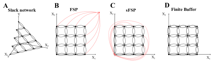
Figure 1: Schematic images of various state-space truncation methods for a CRN with two species: (a) Slack network (this paper), (c) Finite State Projection (FSP) [32], (c) Stationary Finite State Projection (sFSP) [16], (d) Finite Buffer Method [7, 8].

3.2 Algorithm for constructing a network with slack reactants

In general, by using slack reactants, any conservative laws can be deduced in a similar fashion to encode the desired truncation directly in the CRN. We have found this perspective to be advantageous with respect to studying complex CRNs. Rather than thinking about the software implementation of the truncation, it is often easier to design the truncation in terms of slack reactants, then implement the already-truncated system exactly.

We now provide an algorithm to automatically determine the slack reactants required for a specified truncation. It is often the case that a “natural” formulation arises (typically by replacing zero-order complexes with slack reactants) but when that is not the case, one can still find a useful approximation by following our algorithm.

Consider any CRN $(\mathcal{S},\mathcal{C},\mathcal{R},\Lambda)$. Suppose we wish to apply a number of conservation bounds to reduce the state-space of the associated chemical master equation, e.g. many equations of the form

$$w_{i,1}X_{1}+w_{i,2}X_{2}+\dotsc+w_{i,d}X_{d}\leq N_{i},$$ (8)

for $i=1,2,\dots,m$. Collecting the conservation vectors $\{\mathbf{w}_{i}\}_{i=1}^{m}$ into the rows of the $m\times d$ matrix $W$ and each integer $\{N_{i}\}$ into the $m\times 1$ vector $\mathbf{N}$, we may concisely write

$$W\mathbf{X}\preceq\mathbf{N},$$ (9)

where $\preceq$ denotes an element-wise less-than-or-equal operator and $\mathbf{X}$ is the column vector of reactants ${\{X_{i}\}}$.

We augment the $d\times 1$ vector $\mathbf{X}$ with a $m\times 1$ vector $\mathbf{Y}$ of slack reactants to convert the inequality to an equality:

$$\begin{pmatrix}W&I\end{pmatrix}\begin{pmatrix}\mathbf{X}\\ \mathbf{Y}\end{pmatrix}=\mathbf{N},$$ (10)

where $I$ is the $m\times m$ identity matrix. This matrix multiplication implies $m$ conservative laws among $X_{i}$’s and slack reactants $Y_{i}$’s. In other words, we inject the variables $\mathbf{Y}=(Y_{1},Y_{2},\dots,Y_{m})$ into the existing reactions in such a way as to enforce these augmented conservation laws.

To do so, we need to properly define several CRN quantities. Let $S$ be the $|\mathcal{C}|\times|\mathcal{R}|$ connectivity matrix: if the $r$-th reaction establishes an edge from the $i$-th complex to the $j$-th, then $-S_{ir}=S_{jr}=1$ and the other entries in column $r$ are 0. Let $C$ be the $|\mathcal{S}|\times|\mathcal{C}|$ complex matrix $C$. Each column of $C$ corresponds to a unique complex and each row corresponds to a reactant. The entry $C_{ij}$ is the multiplier of $X_{i}$ in complex $j$ (which may be implicitly 0). The stoichiometry matrix is simply ${\Gamma=CS}$, whose $i$-th column indicates the reaction vector of the $i$-th reaction. Note that the CRN admits a conservation law $r_{1}X_{1}(t)+r_{2}X_{2}(t)+\cdots+r_{d}X_{d}(t)=r_{1}X_{1}(0)+r_{2}X_{2}(0)+\cdots+r_{d}X_{d}(0)$ if and only if $\mathbf{r}^{\mkern-2.0mu\top}\Gamma=\mathbf{0}$, where $r=(r_{1},r_{2},\dots,r_{d})^{\mkern-2.0mu\top}$.

Now consider a modified network where we inject $Y_{1},Y_{2},\dots,Y_{K}$ into the complexes. Let $D_{ij}$ denote the (unknown) multiplier of $Y_{i}$ in the $j$-th complex. We require the following to be true:

$$\begin{pmatrix}W&I\end{pmatrix}\begin{pmatrix}C\\ D\end{pmatrix}S=0.$$ (11)

Then by using the same connectivity matrix $S$ and a new complex matrix $\widetilde{C}=\begin{pmatrix}C\\ D\end{pmatrix}$, we obtain a new CRN that enforces the conservative laws (10). To find $D$ satisfying (11), we choose $D$ such that

$$D=U-WC$$ (12)

for an $m\times|\mathcal{C}|$ matrix $U$ with each row of the form $u_{i}\mathbf{1}^{\top}=u_{i}(1,1,\dots,1)^{\mkern-2.0mu\top}$ for some positive integer $u_{i}$. Since $\mathbf{1}^{T}S=\mathbf{0}$, this guarantees (11).

A new network can be generated with the complex matrix $\widetilde{C}$ and the connectivity matrix $S$. We call this network a regular slack network with species $\widetilde{\mathcal{S}}$ and complexes $\widetilde{\mathcal{C}}$. For the $j$-th reaction $\nu_{j}\to\nu^{\prime}_{j}\in\mathcal{R}$ corresponding to the $j$-th column of the matrix $CS$, we denote by $\tilde{\nu}_{j}\to\tilde{\nu}^{\prime}_{j}\in\widetilde{\mathcal{R}}$ the reaction corresponding to the $j$-th column of the matrix $\widetilde{C}S$. That is, $\tilde{\nu}_{j}\to\tilde{\nu}^{\prime}_{j}$ is the reaction obtained from $\nu_{j}\to\nu^{\prime}_{j}$ by adding slack reactants.

We model the slack network by $X^{\mathbf{N}}(t)=(X^{\mathbf{N}}_{1}(t),X^{\mathbf{N}}_{2}(t),\dots,X^{\mathbf{N}}_{d}(t))$ where each of the entries represents the count of species in the new network. Note that the count of each slack reactant $Y_{i}$ is fully determined by species counts $X^{\mathbf{N}}_{i}$’s because of the conservation law(s). As such, we do not explicitly model the $Y_{i}$’s.

The intensity function $\lambda^{\mathbf{N}}_{\tilde{\nu}\to\tilde{\nu}}$ of $X^{\mathbf{N}}$ for a reaction $\tilde{\nu}\to\tilde{\nu}^{\prime}$ is defined as

$$\lambda^{\mathbf{N}}_{\tilde{\nu}\to\tilde{\nu}^{\prime}}(\mathbf{x})=\lambda_{\nu\to\nu^{\prime}}(\mathbf{x})\prod_{i=1}^{m}\mathbbm{1}_{\{y_{i}\geq\tilde{\nu}_{d+1}\}},$$ (13)

where $y_{i}=N_{i}-(w_{i1}x_{1}+w_{i1}x_{1}+\cdots+w_{id}x_{d})$, and $\nu\to\nu^{\prime}$ is the reaction in $\mathcal{R}$. Then we denote by $(\widetilde{\mathcal{S}},\widetilde{\mathcal{C}},\widetilde{\mathcal{R}},\Lambda^{\mathbf{N}})$ a new system with slack reactants obtained from the algorithm, where $\mathcal{K}_{N}$ is the collection of kinetic rates $\{\lambda^{N}_{\tilde{\nu}\to\tilde{\nu}^{\prime}}:\tilde{\nu}\to\tilde{\nu}^{\prime}\in\widetilde{\mathcal{R}}\}$. We refer this system with slack reactants to a slack system.

Here we highlight that the connectivity matrix $S$ and the complex matrix $C$ of the original network are preserved for a new network with slack reactants. Thus the original network and the new network obtained from the algorithm have the same connectivity. This identical connectivity allows the qualitative behavior of the original network, which solely depends on $S$ and $C$, to be inherited to the new network with slack reactants. We particularly exploit the inheritance of accessibility and the inheritance of Poissonian stationary distribution in Section 6.

Remark 3.1.

A single conservation relation, such as $\mathbf{w}\cdot X+y=N$ with a non-negative vector $\mathbf{w}$, is sufficient to truncate the given state space into a finite state space. Hence, in this manuscript, we mainly consider a slack network that is obtained with a single conservation vector $\mathbf{w}$ and a single slack reactant $Y$.

Remark 3.2.

Although we primarily think about bounding our species counts from above, we could also bound species counts from below by choosing negative integers for $w_{i,j}$.

Example 3.1.

We illustrate our slack algorithm with an example CRN consisting of two species and five reactions indicated by edge labels on the following network:

(14)

We enumerate the complexes in the order of $\emptyset,A$ and $B$. We order the reactions according to their labels on the network. Thus the connectivity matrix $S$ and complex matrix $C$ are defined as follows:

$$S=\begin{bmatrix}-1&1&0&0&-1\\ 1&-1&-1&1&0\\ 0&0&1&-1&1\\ \end{bmatrix},$$

$$C=\begin{bmatrix}0&1&0\\ 0&0&1\end{bmatrix}.$$

Suppose we set a conservation bound $A+B\leq N$ for some $N>0$. Then the matrix $A=\begin{bmatrix}1&1\end{bmatrix}$ and by (12), we have $D=\begin{bmatrix}u&u&u\end{bmatrix}-\begin{bmatrix}0&1&1\end{bmatrix}$.

When $u=1$, the network with slack reactant $Y$ is

$$\leavevmode\hbox to61.5pt{\vbox to62.53pt{\text{[drawing]}}}, Y A B Y A B$$ (15)

where we have the conservation relation $A+B+Y=N$, where $N=A(0)+B(0)+Y(0)$.

When $u=2$, the network with slack reactant $Y$ is

$$\leavevmode\hbox to102.32pt{\vbox to79.56pt{\text{[drawing]}}}, 2Y A+Y B+Y 2Y A+Y B+Y$$ (16)

where we have the same conservation relation $A+B+Y=N$.

Here we explain why network (15) is preferred to (16) because it is less intrusive. Let $X=(X_{A},X_{B},X_{Y})$ and $X^{\prime}=(X^{\prime}_{A},X^{\prime}_{B},X^{\prime}_{Y})$ be the stochastic process associated with networks (15) and (16) respectively. Suppose the initial state of both $X$ and $X^{\prime}$ is $(0,0,N)$. $X$ can reach the state $(0,N,0)$ by transitioning $N$ times with the reaction $Y\to B$. This state corresponds to the state $(0,N)$ in the original network (14). On the other hand, $X^{\prime}$ cannot reach the state $(0,N,0)$. This is because the states $(0,0,N)$ and $(0,N-1,1)$ are the only states from which $X^{\prime}$ jumps to $(0,0,N)$. However, no reaction in (16) can be fired at the states since no species $Y$ presents at those states.

Consequently, one state, that is accessible in the original network (14), is lost in the system associated with network (16). However, it can be shown that the stochastic process associated with network (15) preserves all the states of the original network. This occurs mainly because the matrix $D$ for network (15) is sparser than the matrix $D$ for network (16). We discuss how to minimize the effect of slack reactants in Section 3.3.

3.3 Optimal Slack CRNs for effective approximation of the original systems

The algorithm we introduced to construct a network with slack reactants provides is valid and unique up to any user-defined conservation bounds (8), and the outcome is the matrix $D$, shown in (12), that indicates the stoichiometric coefficient of slack reactants at each complex.

As we showed in Example 3.1, to minimize the ‘intrusiveness’ of a slack network, we can simplify a slack network by setting as many ${D_{ij}=0}$ as possible. To do that, we choose the entries of $\mathbf{u}$ such that $u_{i}$ is the maximum entry of the $i$-th row of $AC$. We further optimize the effect of the slack reactants by removing the ‘redundant’ stoichiometric coefficient of slack reactants. For example, for a CRN,

$$\emptyset\rightleftharpoons A\to 2A,$$ (17)

the algorithm generates the following new CRN with a single slack reactant $Y$

$$2Y\rightleftharpoons A+Y\to 2A.$$ (18)

However, by breaking up the connectivity, we can also generate another network

$$Y\rightleftharpoons A,\quad A+Y\to 2A.$$ (19)

The network in (18) is more intrusive than the network in (19) in the sense of accessibility. At any state where $Y=0$, the system associated with (18) will remain unchanged because no reaction can take place. However, the reaction $A\to Y$ in (19) can always occur despite $Y=0$. Hence (19) preserves the accessibility of the original system associated with (17) as any state for $A$ is accessible from any other state in the original reaction system (17). We refer such a system with slack reactants generated by canceling redundant slack reactants to an optimized slack system. In Section 6, we explore the accessibility of an optimized reaction network with slack reactants in a more general setting.

Finally, we can make a network with slack reactants admit a better approximation of a given CRN by choosing an optimized conservation relation in (8). First, we assume that only a single conservation law and a single slack reactant are added to a given CRN. For the purpose of state space truncation onto finitely many states, a single conservation law is enough as all species could be bounded by $N$ as shown in (8). Let this single conservation law be

$$w_{1}X_{1}+w_{2}X_{2}+\cdots w_{d}X_{d}+Y=N.$$

Then the matrix $W$ in (9) is a vector $(w_{1},w_{2},\dots,w_{d})^{\mkern-2.0mu\top}$, and we denote this by $\mathbf{w}$. By the definition of the intensities (13) for a network with slack reactants, some reactions are turned off when $Y=0$, i.e. $w_{1}X_{1}+\dots+w_{d}X_{d}=N$. Geometrically, a reaction outgoing from the hyperplane $w_{1}X_{1}+\dots+w_{d}X_{d}=N$ is turned off (Figure 2).

Hence we optimize the estimation with slack reactants by minimizing such intrusiveness of turned off reactions. To do that, we choose $\mathbf{v}$ which minimizes the number of the reactions in $\{\nu\to\nu^{\prime}\in\mathcal{R}:(\nu^{\prime}-\nu)\cdot\mathbf{w}>0\}$.

Figure 2: The dotted arrows correspond to the reaction vectors that are turned off (i.e. the associated reaction intensity is zero) at the bound of the state space for a slack system as described in Section 3.3.

4 Comparison to Other Truncation-Based Methods

In this Section we demonstrate that our method can potentially resolve limitations in calculating mean first passage times observed in other methods of state space truncation, namely sFSP and the finite-buffer method. Both methods require the user to make decisions about the state-space truncation that may introduce variability in the results. While all methods will converge to the true result as the size of the state space increases, we show our method is less dependent on user defined quantities. This minimizes additional decision-making on the part of the user that can lead to suboptimal results, especially in a context where the solution of the original system is not known.

4.1 Comparison to the sFSP method

A well known state truncation algorithm is known as the Finite State Projection (FSP) method [32]. For a given continuous-time Markov chain, the associated FSP model is restricted to a finite state space. If the process escapes this truncated space, the state is sent to a designated absorbing state (see Figure 1B). For a fixed time $t$, the probability density function of the original system can be approximated by using the associated FSP model with sufficiently many states. The long-term dynamics of the original system, however, is not well approximated because the probability flow of the FSP model leaks to the designated absorbing state in the long run.

To fix this limitation of FSP, Gupta et al. proposed the stationary Finite State Projection method (sFSP)[16]. This method also projects the original state space onto a finite state space as the FSP method intended to. But sFSP does not create a designated absorbing state, as all outgoing transitions from the projected finite state space are merged to a single state $x^{*}$ ‘inside’ the finite state space (Figure 1C). The sFSP has been frequently used to estimate the long-term distribution of discrete stochastic models. However, if the size of the truncated state space is not sufficiently large, this method could fail to provide accurate estimation for the first passage time. To demonstrate this case, we consider the following simple 2-dimensional model. In the network shown in Figure 3A, two $X_{1}$ proteins are dimerized into protein $X_{2}$ while $X_{1}$ is being produced at relatively high rate. The state space of the original model is the full 2-dimensional positive integer grid. We estimate the time until the system reaches one of the two states indicated in red in Figure 3C, and we use alternative methods to do this.

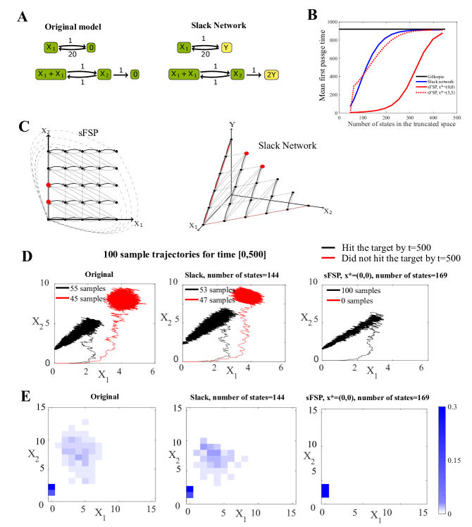
Figure 3: Comparison between an sFSP model and a slack network for the same reaction system. A. Original 2-dimensional system and its slack network. B. Mean first passage time as a function of the truncated state size, comparing sFSP and the slack reactant method. C. The state space truncation corresponding to the sFSP method and the slack method for this model. Target states for the first passage time are indicated in red. D. Mean of 100 sample trajectories obtained by Gillespie simulations for the original, the slack system and the sFSP system. The red lines indicate the mean of the trajectories that have touched the target states within [0,500], while the black lines are the mean of the trajectories that did not touch the target space during this time. E. Probability denstiy heat maps of the stochastic processes modeled under the original, the slack system and the sFSP model, respectively, at $t=500$.

For the sFSP, we project the original state space onto the rectangle by restricting $X_{1}\leq N$ and $X_{2}\leq N$ for some $N>0$, and we fix the origin $(0,0)$ as the designated state $x^{*}$ (Figure 3C). If the process associated with the sFSP model escapes the rectangle, it transports to the designated state immediately. On the other hand, we also consider a slack network shown in Figure 3B, where we introduce the conservation law $X_{1}+2X_{2}+Y=N$ for some $N>0$. Let $\tau=\inf\{t\geq 0:X_{1}=1\text{ and }X_{2}\in\{1,2\}\}$ be the first passage time we want to estimate.

By using the inverse matrix of the truncated transition matrix for each method, as detailed in [9], we obtain the mean of $\tau$ by using different values of $N$. We also obtain an ‘almost’ true mean of $\tau$ by using $10^{5}$ Gillespie simulations of the original process. As shown in Figure 3B, the slack network model provides a more accurate mean first passage time estimation for the size of truncation in between 100 and 400 if the designated return state of sFSP is $(0,0)$.

The inaccurate estimate from the sFSP is due to the choice of a return state. The sFSP model escapes the confined space often because the production rate of $X_{1}$ is relatively high. When it returns back to the origin, it is more likely to visit the target states $\{X_{1}=1\text{ and }X_{2}\in\{1,2\}\}$ than the original process.

Figure 3 shows that the mean first passage time of this system using sFSP depends significantly on the location of the chosen designated state. One of the two states is a particularly poor choice for sFSP, but it illustrates the idea that without previous knowledge of the system it can be difficult to know which states will perform well.

We display the behavior of individual solutions of the original model, the slack network, and the sFSP model in Figure 3D. The trajectory plots show that within the time interval $[0,500]$, almost half of the 100 samples from both the original model and the slack network model stay far away from the target states, while all the 100 sample trajectories from the sFSP model stay close to the target states. We also illustrate this point in Figure 3E with heat maps of the three models at $t=500$. Note that only in the case of the sFSP, the probability densities are concentrated at the target states.

4.2 Comparison to the finite buffer method

The finite buffer method was proposed to estimate the stationary probability landscape with state space truncation and a novel state space enumeration algorithm [7, 8]. For a given stochastic model associated with a CRN, the finite buffer method sets inequalities among species such as (8), so-called buffer capacities. Then at each state $\mathbf{x}$, the transition rate of a reaction $\nu\to\nu^{\prime}$ is set to be zero if at least one of the inequality does not hold at $\mathbf{x}+\nu^{\prime}-\nu$. We note the algorithm, described in Section 3.2, for generating a slack network uses the same inequalities. Thus, the finite buffer method and the slack reactant method truncate the state space in the same way. We have shown, in Section 3.3 this type of truncation can create ‘additional’ absorbing states. These additional absorbing states change the accessibility between the states which means the mean first passage times cannot be accurately estimated. However, the regular slack systems preserve the network structure of the original network. Hence we are able to prove, as we already noted, that regular slack networks inherit the accessibility of the original network as long as the original network is ‘weakly reversible’ as we will define below.

We demonstrate this disparity between the the finite buffer and slack methods with the following network. Consider the mass-action system (14) with a fixed initial state $\mathbf{x}_{0}=(a_{0},b_{0})$. We are interested in estimating the mean first passage time to a target state $\mathbf{x}_{T}=(10,10)$. Note that the state space is irreducible (i.e., every state is accessible from any other state) as the network consists of unions of cycles. This condition, the union of cycles, is precisely what is meant by weakly reversible.[13, 5] Thus, the original stochastic system has no absorbing state and is accessible to the target state $\mathbf{x}_{T}$.

To use the finite buffer method on this network, we set $2X_{A}+X_{B}\leq N$ as the buffer capacity, where $X=(X_{A},X_{B})$ is the associated stochastic process. (Here we choose $N>30$ so the state space contains the target state $\mathbf{x}_{T}$.) Hence when $X$ satisfies $2X_{A}+X_{B}=N$, the reactions $\emptyset\to A$, $B\to A$ and $\emptyset\to B$ cannot be fired as $2X_{A}+X_{B}$ exceeds the buffer capacity. We now demonstrate the system has a new absorbing state. By first using reaction $A\to B$, to deplete all $A$, and then $\emptyset\to B$, every state can reach the state $(0,N)$ in finite time with positive probability. The state $(0,N)$ is absorbing state because no other reactions can occur. Reactions $A\to\emptyset$ and $A\to B$ require at least one $A$ species, and any other reactions lead to states exceeding the buffer capacity. Therefore, the finite buffer method has introduced a new absorbing state not present in the original model so that it is not accessible to $\mathbf{x}_{T}$ with positive probability.

Now, we show the explicit network structure of our slack network formulation will preserve the accessibility of the original system. We consider the same inequality $2X_{A}+X_{B}\leq N$ as above with $N>30$. We generate the slack network by using the algorithm shown in Section 3.2,

(20)

Note that the associated stochastic process $X=(X_{A},X_{B},Y)$ admits the conservation relation $2X_{A}+X_{B}+Y=N$ implying that $2X_{A}+X_{B}\leq N$. The state $(0,N,0)$ can not be reached as the only state that is accessible to $(0,N,0)$ is $(0,N-1,2)$, but it violates the conservation law.

As we highlighted in Section 3.3, slack networks preserve the connectivity of the original network (14), hence the network (20) is also weakly reversible. Thus the state space of the stochastic process associated with the slack network is irreducible by Corollary 6.1. This implies that there is no absorbing state and the system is accessible to $\mathbf{x}_{T}$, unlike the stochastic process associated with the finite buffer relation.

5 Convergence Theorems for slack networks

In this section we establish theoretical results on the convergence of properties of a slack network to the original network. (Proofs of the theorems below are provided in Appendix B.) Many of these results rely on theorems from Hart and Tweedie[18] who studied when the probability density function of a truncated Markov process converges to that of the original Markov process. We employ the same idea of their proof to show the convergence of a slack network to the original network.

By assuming “uniforming mixing,” we show the convergence of the stationary distribution of the slack system to the stationary distribution of the original system as the conservation quantity $N$ grows. Furthermore, we show the convergence of mean first passage times for the slack network to the true mean first passage times. In particular, all these conditions hold when there is a Lyapunov function for the original system.

In this Section, assume that a given CRN $(\mathcal{S},\mathcal{C},\mathcal{R},\Lambda)$ is well defined for all time $t$ and let $(\widetilde{\mathcal{S}},\widetilde{\mathcal{C}},\widetilde{\mathcal{R}},\Lambda^{N})$ be an associated slack network obtained with a single conservative quantity $\mathbf{w}\cdot X\leq N$. We denote by $X$ and $X_{N}$ the associated stochastic processes the original CRN and the slack network respectively. We fix the initial state for both systems, i.e., $X(0)=X_{N}(0)=\mathbf{x}_{0}$ for some $\mathbf{x}_{0}$ and for each $N$. (This means we can only consider slack systems where $N$ is large enough so that $\mathbf{w}\cdot\mathbf{x}(0)<N$.) Assume that both the original and slack systems are irreducible, and denote by $\mathbb{S}$ and $\mathbb{S}_{N}$ the state spaces for each respectively. (In Section 6, we prove accessibility properties that the slack system can inherit from the original system.)

Notice that every state in $\mathbb{S}_{N}$ satisfies our conservation inequality. That is, for every $\mathbf{x}\in\mathbb{S}_{N}$ we have $\mathbf{w}\cdot\mathbf{x}\leq N$. It is possible that $\mathbb{S}_{N}=\mathbb{S}_{N+1}$ for some $N$. For simplicity, we assume that the truncated state space is always enlarged with respect to the conservative quantity $N$, that is $\mathbb{S}_{N}\subset\mathbb{S}_{N+1}$ for each $N$. (For the general case, we could simply consider a subsequence $N_{k}$ such that $N_{k}<N_{k+1}$ and $\mathbb{S}_{N_{k}}\subset\mathbb{S}_{N_{k+1}}$ for each $k$.)

As defined in Section 2, $\lambda_{\nu\to\nu^{\prime}}\in\Lambda$ is the intensity of a reaction $\nu\to\nu^{\prime}$ for the associated stochastic system $X$. We also denote by $\lambda^{N}_{\tilde{\nu}\to\tilde{\nu}^{\prime}}\in\Lambda^{N}$ the intensity of a reaction $\tilde{\nu}\to\tilde{\nu}^{\prime}$ for the associated stochastic system $X_{N}$. Finally we let $p(\mathbf{x},t)$ and $p_{N}(\mathbf{x},t)$ be the probability density function of $X$ and $X_{N}$, respectively. We begin with the convergence of the probability density functions of the slack network to the original network with increasing $N$.

Theorem 5.1.

For any $\mathbf{x}\in\mathbb{S}_{N}$ and $t\geq 0$, we have

$$\lim_{N\to\infty}|p(\mathbf{x},t)-p_{N}(\mathbf{x},t)|=0.$$

A Markov process defined on a finite state space admits a stationary distribution. Hence $X_{N}$ admits a stationary distribution $\pi_{N}$. If the slack system satisfies the condition of “uniform mixing”, that is the convergence rate of $\|p_{N}(\mathbf{x},t)-\pi_{N}(\mathbf{x})\|_{1}$ is uniform in $N$, then we have the following result:

Theorem 5.2.

Suppose $X$ admits a stationary distribution $\pi$. Suppose further that there exists a positive function $h(t)$, which is independent of $N$, such that $\|p_{N}(\cdot,t)-\pi_{N}\|_{1}\leq h(t)$ and $\displaystyle\lim\limits_{t\to\infty}h(t)=0$. Then

$$\lim_{N\to\infty}\|\pi-\pi_{N}\|_{1}=0.$$

We now consider convergence of the mean first passage time of $X_{N}$. Recall, we assumed that both stochastic processes have the same initial state $X(0)=X_{N}(0)=\mathbf{x}_{0}$ and both state spaces $\mathbb{S}$ and $\mathbb{S}_{N}$ are irreducible. Hence, for any $K\subseteq\mathbb{S}$, each state in $\mathbb{S}_{N}$ is accessible to $K$ for sufficiently large $N$.

Theorem 5.3.

For a subset $K$ of the state space of $X$, let $\tau$ and $\tau_{N}$ be the first passage times to $K$ for $X$ and to $K\cap\mathbb{S}_{N}$ for $X_{N}$, respectively. Assume the following conditions,

1. $X$ admits a stationary distribution $\pi$, and

2. $\displaystyle\lim\limits_{N\to\infty}\|\pi-\pi_{N}\|_{1}=0$.

Then for any $t\geq 0$,

$$\lim_{N\to\infty}|P(\tau>t)-P(\tau_{N}>t)|=0.$$

If we further assume that

1. $E(\tau)<\infty$, and

2. there exists $g(t)$ such that $P(\tau_{N}>t)\leq g(t)$ for all $N$ and $\int_{0}^{\infty}g(t)dt<\infty$,

then

$$\lim_{N\to\infty}|E(\tau)-E(\tau_{N})|=0.$$

Remark 5.1.

To obtain convergence of higher moments of the first passages time, we need only replace conditions $E(\tau_{K})<\infty$ and $\int_{0}^{\infty}g(t)dt<\infty$ with

$$E(\tau^{n}_{K})<\infty\quad\text{and}\quad\int_{0}^{\infty}g\left(t^{\frac{1}{n}}\right)dt<\infty,$$ (21)

respectively.

We now show that if a Lyapunov function exists for the original system, the conditions in Theorem 5.2 and Theorem 5.3 hold. The Lyapunov function approach has been proposed by Meyn and Tweedie [31] and it has been used to study long-term dynamics of Markov processes [6, 16, 4, 17] especially exponential ergodicity. Gupta et al [16] uses a linear Lyapunov function to show that the stationary distribution of an sFSP model converges to a stationary distribution of the original stochastic model and use the Lyapunov function explicitly compute the convergence rate. In particular, we show Lyapunov functions exist for the examples we consider in Section 7.

Theorem 5.4.

Suppose there exists a function $V$ and positive constants $C$ and $D$ such that for all $\mathbf{x}$,

1. $V(\mathbf{x})\geq 1$ for all $\mathbf{x}\in\mathbb{S}$,

2. $V$ is an increasing function in the sense that

   $$V(\mathbf{x}_{N+1})\geq V(\mathbf{x}_{N})$$

   for each $\mathbf{x}_{N+1}\in\mathbb{S}_{N+1}\setminus\mathbb{S}_{N}$ and $\mathbf{x}_{N}\in\mathbb{S}_{N}$, and

3. $\displaystyle\sum\limits_{\nu\to\nu^{\prime}\in\mathcal{R}}\lambda_{\nu\to\nu^{\prime}}(\mathbf{x})(V(\mathbf{x}+\mathbf{\nu}^{\prime}-\mathbf{\nu})-V(\mathbf{x}))$

   $$\leq-CV(\mathbf{x})+D.$$

Then the conditions in Theorem 5.3 hold.

Remark 5.2.

The conditions (21) hold if a Lyapunov function satisfying the conditions in Theorem 5.4 exists. Thus, the convergence of the higher moments of the first passage time also follows.

6 Inheritance of slack networks

As we showed in Section 4.2, not all state space truncations preserve accessibility of states in the original system. (For the example in Section 4.2, the truncation created a new absorbing state.) Thus, it is desirable to obtain reduced models that are guaranteed to maintain the accessibility of the original system to predetermined target states. In this Section, we show that under mild conditions, both a regular slack system and an optimized slack system preserve the original accessibility. The proofs of the theorems introduced in this section are in Appendix C. The key to these results is the condition of weak reversibility.

Definition 6.1.

A reaction network is weakly reversible if each connected component of the network is strongly connected. That is, if there is a path of reactions from a complex $\nu$ to $\nu^{\prime}$, then there is a path of reactions $\nu^{\prime}$ to $\nu$.

We note that the weakly reversible condition applies to the network graph of the CRN. The network graph consists of complexes (nodes) and reactions (edges). It is a sufficient condition for irreducibility of the associated mass-action stochastic process. Indeed, the sufficiency of weak reversibility holds even under general kinetics as long as condition (4) is satisfied.[33] Hence irreducibility of a regular slack network follows since it preserves weak reversibility of the original network and the kinetics modeling the regular slack system satisfies (4).

Corollary 6.1.

Let $(\mathcal{S},\mathcal{C},\mathcal{R},\Lambda)$ be a weakly reversible CRN with intensity functions $\Lambda=\{\lambda_{y\to y^{\prime}}\}$ satisfying (4). Then the state space of the associated stochastic process with a regular slack network $(\widetilde{\mathcal{S}},\widetilde{\mathcal{C}},\widetilde{\mathcal{R}},\Lambda^{N})$ is a union of closed communication classes for any $N$.

In case the original network is not weakly reversible, we can still guarantee that optimized slack systems have the same accessibility as the original system provided all species have a degradation reaction ($S_{i}\to\emptyset$).

Theorem 6.1.

Let $(\mathcal{S},\mathcal{C},\mathcal{R},\Lambda)$ be a reaction network such that $\{S_{i}\to\emptyset:S_{i}\in\mathcal{S}\}\subset\mathcal{R}$. Suppose that the stochastic process $X$ associated with $(\mathcal{S},\mathcal{C},\mathcal{R},\Lambda)$ and beginning at the point $\mathbf{x}_{0}$ is irreducible. Let $X_{N}$ be the stochastic process associated with an optimized slack network $(\widetilde{\mathcal{S}},\widetilde{\mathcal{C}},\widetilde{\mathcal{R}},\Lambda^{N})$ such that $X_{N}(0)=\mathbf{x}_{0}$ for every $N$ large enough. Then, for any subset $K$ of the state space of $X$, there exists $N_{0}$ such that $X_{N}$ reaches $K$ almost surely for $N\geq N_{0}$.

This theorem follows from the fact that a slack system only differs from the original system when its runs out of slack reactants. However, in an optimized slack system, degradation reactions are allowable with no slack reactants. Hence, our proof of Theorem 6.1 relies on the presence of all degradation reactions.

A slack network may also inherit its stationary distribution from the original reaction system. When the original system admits a stationary distribution of a product form of Poissons under the complex balance condition, a slack system inherits the same form of the stationary distribution as well. A reaction system is complex balanced if the associated deterministic mass-action system admits a steady state $c^{*}$, such that

$$\sum_{\begin{subarray}{c}\nu\in\mathcal{C}\\ \nu\to\nu^{\prime}\in\mathcal{R}\end{subarray}}f_{\nu}(\mathbf{c}^{*})=\sum_{\begin{subarray}{c}\nu^{\prime}\in\mathcal{C}\\ \nu\to\nu^{\prime}\in\mathcal{R}\end{subarray}}f_{\nu^{\prime}}(\mathbf{c}^{*}),$$

where $f_{\nu}(x)=x_{1}^{\nu_{1}}\cdots x_{d}^{\nu_{d}}$ is the deterministic mass-action rate [12]. If a reaction system is complex balanced, then its associated stochastic mass-action system admits a stationary distribution corresponding to a product of Poisson distributions centered at the complex balance steady state.[3]. The following lemma show that the complex balancing of the original network is inherited by a regular slack network.

Lemma 6.1.

Suppose that $(\mathcal{S},\mathcal{C},\mathcal{R},\Lambda)$ is a reaction network whose mass-action deterministic model admits a complex balanced steady state $c^{*}$. Then any regular slack network $(\widetilde{\mathcal{S}},\widetilde{\mathcal{C}},\widetilde{\mathcal{R}},\Lambda^{N})$ with slack reactants $Y_{1},\cdots,Y_{m}$ also admits a complex balanced steady state at $\tilde{c}=(c^{*},1,1,\dots,1)^{\top}$.

Remark 6.1.

Note that a regular slack network also preserves the deficiency of the original network. Deficiency $\delta$ of a reaction network is an index such that

$$\delta=n-\ell-s,$$

where $n$ is the number of the complexes, $\ell$ is the number of connected components and $s$ is the rank of the stoichiometry matrix of the reaction network. Deficiency characterizes the connectivity of the network structure, and surprisingly it can also determine the long-term behavior of the system dynamics regardless of the system parameters.[12, 20, 3] A regular slack network and original network have the same number of complexes $n$, and the same connectivity matrix $S$, which implies they have the same number of connected components $\ell$. Furthermore, using the notation from Section 3.2, the stoichiometry matrices are $\Gamma=CS$ for the original network and

$$\widetilde{\Gamma}=\begin{pmatrix}C\\ U-AC\end{pmatrix}S=\begin{pmatrix}CS\\ -WCS\end{pmatrix}$$

for a slack network, which means that they have the same rank $s$. Together, these imply that the original network and its regular slack network have the same deficiency.

Since the complex balancing is inherited with the same steady state values for $X_{i}$, we have the following stochastic analog of inheritance of the Poissonian stationary distribution for regular slack systems.

Theorem 6.2.

Let $X$ be the stochastic mass-action system associated with a complex balanced $(\mathcal{S},\mathcal{C},\mathcal{R},\Lambda)$ with an initial condition $X(0)=\mathbf{x}_{0}$. Let $X_{N}$ be the stochastic system associated with a regular slack system $(\widetilde{\mathcal{S}},\widetilde{\mathcal{C}},\widetilde{\mathcal{R}},\Lambda^{N})$ with $X_{N}(0)=\mathbf{x}_{0}$. Then, for the state space $\mathbb{S}_{N}$ of $X_{N}$, there exists a constant $M_{N}>0$ such that

$$\pi_{N}(\mathbf{x})=M_{N}\pi(\mathbf{x})\quad\text{for $\mathbf{x}\in\mathbb{S}_{N}$,}$$

where $\pi$ and $\pi_{N}$ are the stationary distributions of $X$ and $X_{N}$, respectively.

We demonstrate Lemma 6.1 and Theorem 6.2 with a simple example.

Example 6.1.

Consider two networks,

$$X\xrightleftharpoons[2]{1}0,$$ (22)

$$X\xrightleftharpoons[2]{1}Y.$$ (23)

Let $X$ and $X_{N}$ be systems (22) and (23), respectively, where $N$ is the conservation quantity $X_{N}(t)\leq N$. Under mass-action kinetics, the complex balance steady state of (22) is $c^{*}=2$. Under mass-action kinetics, $\tilde{c}=(2,1)$ is a complex balance steady state of (23).

Now let $\pi$ and $\pi_{N}$ be the stationary distribution of $X$ and $X_{N}$, respectively. By Theorem 6.4, Anderson et al [3], $\pi$ is a product form of Poissons such that

$$\pi(x)=e^{-2}\frac{{c^{*}}^{x}}{x!}\quad\text{for each state $x$}.$$

By plugging $\pi$ into the chemical master equation 3 of $X_{N}$ and showing that for each $\mathbf{x}$

$$\lambda^{N}_{X\to Y}(\mathbf{x}+1)\pi(\mathbf{x}+1)+\lambda^{N}_{Y\to X}(\mathbf{x}-1)\pi(\mathbf{x}-1)$$

$$=(x+1)\mathbbm{1}_{\{N-x-1\geq 0\}}e^{-2}\frac{2^{x+1}}{(x+1)!}+2\mathbbm{1}_{\{N-x+1\geq 1\}}e^{-2}\frac{2^{x-1}}{(x-1)!}$$

$$=x\mathbbm{1}_{\{N-x\geq 0\}}e^{-2}\frac{2^{x}}{x!}+2\mathbbm{1}_{\{N-x\geq 1\}}e^{-2}\frac{2^{x}}{x!}$$

$$=\lambda^{N}_{X\to Y}(\mathbf{x})\pi(\mathbf{x})+\lambda^{N}_{Y\to X}(\mathbf{x})\pi(\mathbf{x})$$

we can verify that $\pi$ is a stationary solution of the chemical master equation 3 of $X_{N}$. Since the state space of $X_{N}$ is $\{x\in\mathbb{Z}_{\geq 0}:x\leq N\}$, we choose a constant $M_{N}$ such that

$$\sum_{0\leq x\leq N}M_{N}\pi(x)=1.$$

Then $\pi_{N}=M_{N}\pi$ is the stationary distribution of $X_{N}$.

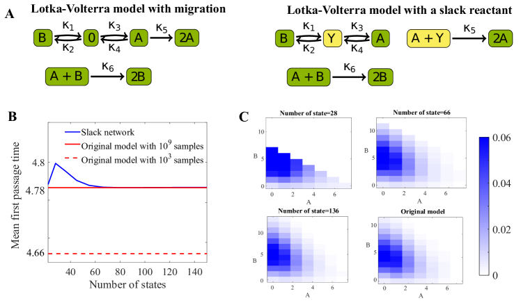
Figure 4: Calculating Mean Time to Extinction of a Lotka-Volterra Model with Migration Using Slack Reactants. A. The reaction network for the Lotka-Volterra model with migration (left). The Lotka-Volterra model with a slack reactant $Y$ (right). The parameters are $\kappa_{1}=0.1,\kappa_{2}=0.1,\kappa_{3}=0.2,\kappa_{4}=0.6,\kappa_{5}=0.2$ and $\kappa_{6}=0.2$. B. Convergence of the mean time to extinction of the slack network (blue) to the true network (solid red). C. Heatmaps of the probability density at time $1000$ of the original model and the slack system with various truncation size.

7 Applications of Slack Networks

In this Section, we demonstrate the utility of slack reactants in computing mean first-passage times for two biological examples. For both examples, we compute the mean first passage time via the matrix inversion approach as shown in Appendix A.

7.1 A Lotka-Volterra model with migration

Consider a Lotka-Volterra model with migration shown in Figure 4A. In this model, species $A$ is the prey, and species $B$ is the predator. Clearly, the state space this model is infinite $(A,B)$ such that $A\geq 0$, $B\geq 0$. We will use slack reactants to determine the expected time to extinction of either species. More specifically, let $K=\{(A,B):A=0\text{ or }B=0\}$. We will calculate the mean first arrival time to $K$ from an initial condition $(A(0),B(0))$. (In our simulations in Figure 4, we chose $(A(0),B(0))=(3,3)$.)

To generate our slack network, we choose a conservative bound $w\cdot(A,B)^{\top}\leq N$ with $w=(1,1)$. As we discussed in Section 3.3, this $w$ minimizes the intrusiveness of slack reactants because the number of reactions $\nu\to\nu^{\prime}$ such that $(\nu^{\prime}-\nu)\cdot w>0$ is minimized. By using the algorithm introduced in Section 3.2, we generate a regular slack network (LABEL:eq:regular_slack) with a slack reactant $Y$,

$$\begin{split}&B+Y\xrightleftharpoons[\kappa_{2}]{\kappa_{1}}2Y\xrightleftharpoons[\kappa_{4}]{\kappa_{3}}A+Y\xrightarrow{\kappa_{5}}2A,\\ &A+B\xrightarrow{\kappa_{6}}2B.\end{split}$$ (24)

As the slack reactant $Y$ in reactions $B+Y\rightleftharpoons 2Y\rightleftharpoons A+Y$ can be canceled, we further generate the optimized slack network shown in Figure 4A. We let $A(0)+B(0)+Y(0)=N$, which is the conservation quantity of the new network.

Let $\tau$ be the first passage time from our initial condition to $K$. First, we examine the accessibility of the set $K$. Because our reaction network contains creation and destruction of all species (i.e., $B\rightleftharpoons\emptyset\rightleftharpoons A$) the original model is irreducible and any state is accessible to $K$. Furthermore, Theorem 6.1 guarantees that the stochastic model associated with the optimized slack network is also accessible to $K$ from any state.

Next, by showing there exists a Lyapunov function satisfying the condition of Theorem 5.4 for the original model, we are guaranteed the first passages times from our slack network will converge to the true first passage times. (See Appendix E.1 for more detail.) Therefore, as the plot shows in Figure 4B, the mean first extinction time of the slack network converges to that of the original model, as $N$ increases. The mean first passage time of the original model was obtained by averaging $10^{9}$ sample trajectories. These trajectories were computed serially on a commodity machine and took $4.6$ hours to run. In contrast, the mean first passage times of the slack systems were computed analytically on the same computer and took at most 13 seconds. Figure 4 also shows that using only $10^{3}$ samples is misleading as the simulation average has not yet converged to the true mean first passage time. Finally, as expected from Theorem 5.1 the probability density of the slack network converges to that of the original network (see Figure 4C).

7.2 Protein synthesis with slow toggle switch

We now consider a protein synthesis model with a toggle switch, see Figure 5A. Protein species $X$ and $Z$ may be created, but only when their respective genes $D^{X}$ or $D^{Z}$ are in the active (unoccupied) state, $D^{X}_{0}$ and $D^{Z}_{0}$. Each protein acts as a repressor for the other by binding at the promoter of the opposite gene and forcing it into the inactive (occupied) state ($D^{X}_{1}$ and $D^{Z}_{1}$). In this system we consider only one copy of each gene, so that, $D^{X}_{0}+D^{X}_{1}=D^{Z}_{0}+D^{Z}_{1}=1$ for all time. Thus, we focus primarily on the state space of protein numbers only $(X,Z)$.

The deterministic form of such systems are often referred to as a “bi-stable switch” as it is characterized by steady states $(X^{*},0)$ and ($X$ “on” and $Z$ “off”) and $(0,Z^{*})$ ($X$ “off” and $Z$ “on”). This stochastic form of toggle switch has been shown to exhibit a multi-modal long-term probability density due to switches between these two deterministic states due to rapid significant changes in the numbers of proteins $X$ and $Z$ by synthesis or degradation (depending on the state of promoters) [1]. Figure 5C shows that the associated stochastic system admits a tri-modal long-term probability density. Thus the system transitions from one mode to other modes and, for the kinetic parameters chosen in Figure 5, rarely leaves the region $R=\{(X,Z)|0\leq X\leq 30\text{ or }0\leq Z\leq 30\}$. Significant departures from a stable region of a genetic switch may be associated with irregular and diseased cell fates. As such, the first passage time of this system outside of $R$ may indicate the appearance of an unexpected phenotype in a population. Because this event is rare, estimating first passage times with direct stochastic simulations, such as with the Gillespie algorithm [15], will be complicated by the long time taken to exit the region.

As in the previous example, slack systems provide a valuable tool for direct calculation of mean first passage times. In this example, we consider the time a trajectory beginning at state $(X,Z,D^{X}_{0},D^{Z}_{0})=(0,0,1,1)$ enters the target set $K=\{(X,Z)|X>30\text{ and }Z>30\}=R^{c}$ and compute $\tau$, the first passage time to $K$.

Since the species corresponding to the status of promoters ($D^{X}_{0},D^{X}_{1},D^{Z}_{0}$ and $D^{Z}_{1}$) are already bounded, we use the conservative bound $X+Z\leq N$ to generate a regular slack network in Figure 5B with the algorithm introduced in Section 3.2. The original toggle switch model is irreducible (because of the degradation $X\to 0$, $Z\to 0$ and protein synthesis $Z+D^{X}_{0}\leftarrow D^{X}_{1}$, $X+D^{Z}_{0}\leftarrow D^{Z}_{1}$ reactions). Moreover by Theorem 6.1, the degradation reactions guarantee that the slack system is also accessible to $K$ from any state.

As shown in Figure 5D, the mean first passage time of the slack system appears to be converting to approximately $3.171\times 10^{9}$. To prove that the limit of the slack system is actually the original mean first passage time, we construct a Lyapunov functions satisfying the conditions of Theorem 5.4. See Appendix E.2 for more details about the construction of the Lyapunov function.

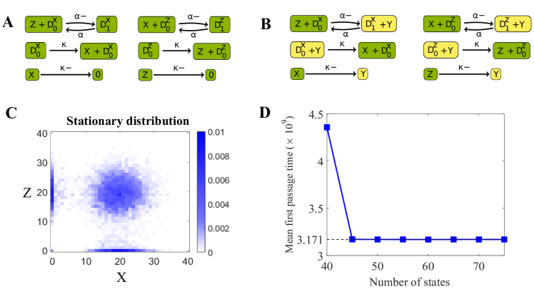
Figure 5: Calculating Mean First Passage Time of a Slow Toggle Switch Using Slack Reactants. A. Protein synthesis with slow toggle switch. B. The toggle switch model with a slack reactant $Y$. Parameters are $\alpha-=0.1,\alpha=10,\kappa=2000$ and $\kappa-=100$. C. Multimodal long-term probability distribution of the original model. D. Convergence of the first passage time of the slack system with various truncation sizes.

8 Discussion & Conclusions

We propose a new state space truncation method for stochastic reaction networks (see Section 3). In contrast to other methods, such as FSP, sFSP and the finite buffer method, we truncate the state space indirectly by expanding the original chemical reaction network to include slack reactants. The truncation is imposed through user defined conservation relations among species. The explicit network structure of slack reactants facilitates proofs of convergence (Section 5) and allows the use of existing software packages to study the slack network itself [23]. Indeed, any user-defined choices for conservation laws, conservation amounts, and stochiometric structure, can be used to construct a slack network with our algorithm. We provide guidelines for optimal user choices that can increase the similarity between the slack system and the original model (see Section 3.3).

Slack systems can be used to estimate the dynamical behavior of the original stochastic model. In Section 4, we used a simple example to show that the slack method can lead to a better approximation for the mean first passage time than the sFSP method and the finite buffer method. In particular, in Section 5 we provide theorems that show the slack system approximates the probability density and the mean first passage time of the original system. Because slack networks preserve network properties, such as weak reversibility, the slack system is also likely to have the same accessibility to a target state as the original model (see Section 6). In particular, we note that weak reversibility guarantees our slack truncation does not introduce absorbing states.

In Section 6, we show that this truncation method is natural in the sense that the stationary distributions of the original and slack system are identical up to multiplication by a constant when the original system is complex balanced. Finally, in Section 7, we use slack networks to calculate first passage times for two biological examples. We expect that this new theoretical framework for state space truncation will be useful in the study of other biologically motivated stochastic chemical reaction systems.

Data Availability

The data that support the findings of this study are available from the corresponding author upon reasonable request.

Appendix A First passage time for Markov processes with finitely many states

The Markov chain associated with a slack network has always a finite state space. There are many different methods to analytically derive the mean first passage time of a Markov chain with a finite state space [22, 21, 37, 9]. In this paper, we use the method of Laplace transform which is also used in [37].

For a continuous time Markov process, let $\mathbb{S}$ be the finite state space and let $Q$ be the transition rate matrix, i.e. $Q_{ij}$ is the transition rate from state $i$ to state $j$ if $i\neq j$ and $Q_{ii}=-\sum_{j\neq i}Q_{ij}$.

For a subset $K=\{i_{1},i_{2},\dots,i_{k}\}\subset\mathbb{S}$, we define a truncated transition matrix $Q_{K}$ that is obtained by removing the $i_{j}$ th row and column from $Q$ for $j=1,2,\dots,k$. Then the mean first passage time to set $K$ starting from the $i$-th state is the $i$-th entry of $-Q_{K}^{-1}\mathbf{1}$, where $\mathbf{1}$ is a column vector with each entry $1$.

Appendix B Proofs of Convergence Theorems

In this section, we provide the proofs of the theorems introduced in Section 5. We use the same notations and the same assumptions as we used in Section 5.

Proof of Theorem 5.1: We employ the main idea shown in the proof of Theorem 2.1 in Hart and Tweedie [18]. Let a state $\mathbf{x}$ and time $t$ be fixed. We consider large enough $N$ so that $\mathbf{x}\in\mathbb{S}_{N-1}$.

We use an FSP model on $\mathbb{S}_{N-1}$ of the original system $X$ with the designated absorbing state $\mathbf{x}^{*}\in\mathbb{S}_{N-1}^{c}$. Let $p^{\text{FSP}}_{N-1}$ be the probability density function of this FSP model.

Let $T_{N}$ be the first time for $X_{N}$ to hit $\mathbb{S}_{N}\setminus\mathbb{S}_{N-1}$. We generate a coupling of $X_{N}$ and the FSP model restricted on $\mathbb{S}_{N-1}$ as they move together by $T_{N}$ and they move independently after $T_{N}$. Then $p^{\text{FSP}}_{N-1}(\mathbf{x},t)=P(X_{N}(t)=\mathbf{x},T_{N}>t)$ for $\mathbf{x}\in\mathbb{S}_{N-1}$ because the FSP model has stayed in $\mathbb{S}_{N-1}$ if and only if $X_{N}$ has never touched $\mathbb{S}_{N}\setminus\mathbb{S}_{N-1}$. Thus

$$p_{N}(\mathbf{x},t) =P(X_{N}(t)=\mathbf{x},t<T_{N})+P(X_{N}(t)=\mathbf{x},t\geq T_{N})$$

$$=p^{\text{FSP}}_{N-1}(\mathbf{x},t)+P(X_{N}(t)=\mathbf{x},T_{N}\leq t)$$ (25)

$$\geq p^{\text{FSP}}_{N-1}(\mathbf{x},t).$$

Furthermore

$$P(X_{N}(t)=\mathbf{x},t\geq T_{N})\leq P(t\geq T_{N})$$

$$=p^{\text{FSP}}_{N-1}(\mathbf{x}^{*},t)=1-p^{\text{FSP}}_{N-1}(\mathbb{S}_{N-1},t),$$

where we used the fact that after $T_{N}$, the FSP process is absorbed at $\mathbf{x}^{*}$. Thus

$$p^{\text{FSP}}_{N-1}(\mathbf{x},t)\leq p_{N}(\mathbf{x},t)\leq p^{\text{FSP}}_{N-1}(\mathbf{x},t)+1-p^{\text{FSP}}_{N-1}(\mathbb{S}_{N-1},t).$$ (26)

Note that

$$p^{\text{FSP}}_{N-1}(\mathbf{x},t)=P(X(t)=\mathbf{x},t<T_{N})\leq p(\mathbf{x},t).$$

Since $T_{N}$ increases to $\infty$ almost surely, as $N$ increases, $p^{\text{FSP}}_{N-1}(\mathbf{x},t)$ monotonically increases in $N$ and converges to $p(\mathbf{x},t)$, as $N\to\infty$ for each $\mathbf{x}\in\mathbb{S}_{N}$. Then by using the monotone convergence theorem, the term

$$p^{\text{FSP}}_{N-1}(\mathbb{S}_{N-1},t)=\sum_{x\in\mathbb{S}}p^{\text{FSP}}_{N-1}(x,t)\mathbbm{1}_{\{x\in\mathbb{S}_{N-1}\}}$$

converges to $p(\mathbb{S},t)=1$. Therefore, by taking $\displaystyle\lim\limits_{N\to\infty}$ in both sides of (26) the result follows. $\square$

Proof of Theorem 5.2: This proof is a slight generalization of the proof of Theorem 3.3 in Hart and Tweedie [18]. Since the convergence of $\|p_{N}(\cdot,t)-\pi_{N}\|_{1}$ is independent of $N$, for any $\epsilon>0$, we choose sufficiently large $t_{0}$ such that

$$\|p(\cdot,t_{0})-\pi(t_{0})\|_{1}\leq\epsilon\quad\text{and}\quad\|p_{N}(\cdot,t_{0})-\pi_{N}(t_{0})\|_{1}\leq\epsilon$$

for all $N$. Then by using the triangle inequalities

$$\|\pi-\pi_{N}\|_{1} \leq\|p(\cdot,t_{0})-\pi\|_{1}+\|p_{N}(\cdot,t_{0})-\pi_{N}\|_{1}$$

$$\ \ +\|p(\cdot,t_{0})-p_{N}(\cdot,t_{0})\|_{1}$$

$$\leq\|p(\cdot,t_{0})-\pi\|_{1}+\|p_{N}(\cdot,t_{0})-\pi_{N}\|_{1}$$

$$\ \ +\|p(\cdot,t_{0})-p^{\text{FSP}}_{N-1}(\cdot,t_{0})\|_{1}$$

$$\ \ +\|p^{\text{FSP}}_{N-1}(\cdot,t_{0})-p_{N}(\cdot,t_{0})\|_{1}$$

$$\begin{split}&\leq 2\epsilon+\sum_{\mathbf{x}\in\mathbb{S}}|p(\mathbf{x},t_{0})-p^{\text{FSP}}_{N-1}(\mathbf{x},t_{0})|\\ &\ \ +\sum_{x\in\mathbb{S}}|p^{\text{FSP}}_{N-1}(\mathbf{x},t_{0})-p_{N}(\mathbf{x},t_{0})|.\end{split}$$ (27)

Note that as we mentioned in the proof of Theorem 5.1, we have monotone convergence of $p^{\text{FSP}}_{N-1}(\mathbf{x},t_{0})$ to $p(\mathbf{x},t_{0})$ for each $\mathbf{x}\in\mathbb{S}_{N-1}$, as $N\to\infty$. Hence by the monotone convergence theorem, the first summation in (LABEL:eq:conv_of_mfpt_final) goes to zero, as $N\to\infty$. Note further that from (25) we have

$$|p^{\text{FSP}}_{N-1}(\mathbf{x},t_{0})-p_{N}(\mathbf{x},t_{0})|=P(X_{N}(t)=\mathbf{x},T_{N}\leq t_{0}).$$

Hence the second summation in (LABEL:eq:conv_of_mfpt_final) satisfies

$$\sum_{x\in\mathbb{S}}|p^{\text{FSP}}_{N-1}(\mathbf{x},t_{0})-p_{N}(\mathbf{x},t_{0})| \leq\sum_{x\in\mathbb{S}_{N-1}}|p^{\text{FSP}}_{N-1}(\mathbf{x},t_{0})-p_{N}(\mathbf{x},t_{0})|$$

$$\ \ +p^{\text{FSP}}_{N-1}(x^{*},t_{0})$$

$$\ \ +P(X_{N}(t)\in\mathbb{S}_{N}\setminus\mathbb{S}_{N-1}).$$

Note that by (25)

$$\sum_{x\in\mathbb{S}_{N-1}}|p^{\text{FSP}}_{N-1}(\mathbf{x},t_{0})-p_{N}(\mathbf{x},t_{0})|$$

$$=\sum_{x\in\mathbb{S}_{N-1}}P(X_{N}(t_{0})=\mathbf{x},t_{0}\geq T_{N})=P(t_{0}\geq T_{N})$$

Furthermore $p^{\text{FSP}}_{N-1}(x^{*},t_{0})=P(t_{0}\geq T_{N})$ and $P(X_{N}(t)\in\mathbb{S}_{N}\setminus\mathbb{S}_{N-1})=P(T_{N}<t_{0})$. Hence $\sum_{x\in\mathbb{S}}|p^{\text{FSP}}_{N-1}(\mathbf{x},t_{0})-p_{N}(\mathbf{x},t_{0})|\to 0$, as $N\to\infty$ because $T_{N}\to\infty$ almost surely, as $N\to\infty$.

Consequently, we have

$$\lim_{N\to\infty}\|\pi-\pi_{N}\|_{1}\leq 2\epsilon.$$

Since we choose an arbitrary $\epsilon$, the completes the proof. $\square$

In order to prove Theorem 5.3, we consider an ‘absorbing’ Markov process associated with $X$ and $X_{N}$. Let $\bar{X}$ and $\bar{X}_{N}$ be Markov processes such that

$$\bar{X}(t)=\begin{cases}X(t)&\text{ if $t<\tau$,}\\ X(\tau)&\text{ if $t\geq\tau$}.\end{cases}$$

$$\bar{X}_{N}(t)=\begin{cases}X_{N}(t)&\text{ if $t<\tau_{N}$,}\\ X_{N}(\tau_{N})&\text{ if $t\geq\tau_{N}$}.\end{cases}$$

That is, $\bar{X}$ and $\bar{X}_{N}$ are coupled process to $X$ and $X_{N}$, respectively. Furthermore they are absorbed to $K$ once the coupled process ($X$ for $\bar{X}$ and $X_{N}$ for $\bar{X}_{N}$) visits the set $K$. These coupled process have the following relation.

Lemma B.1.

Let $t\geq 0$ be fixed and $\epsilon>0$ be arbitrary. Suppose $X$ admits a stationary distribution $\pi$. Suppose further that $\displaystyle\lim\limits_{N\to\infty}\|\pi-\pi_{N}\|_{1}=0$. Then there exists a finite subset $\bar{K}$ such that $P(\bar{X}(t)\in\bar{K}^{c})<\epsilon$ and $P(\bar{X}_{N}(t)\in\bar{K}^{c})<\epsilon$ for sufficiently large $N$.

Proof.

Since the probabilities of $\bar{X}$ and $\bar{X}_{N}$ are leaking to $K$, we have for each $t$ and for each $\mathbf{x}\in K^{c}$

$$\begin{split}&P(\bar{X}(t)=\mathbf{x})\leq P(X(t)=\mathbf{x}),\quad\text{and}\\ &P(\bar{X}_{N}(t)=\mathbf{x})<P(X_{N}(t)=\mathbf{x}).\end{split}$$ (28)

This can be formally proved as for each $x\in K^{c}$

$$P(X(t)=\mathbf{x}) =P(X(t)=\mathbf{x},\tau>t)+P(X(t)=\mathbf{x},\tau\leq t)$$

$$=P(\bar{X}(t)=\mathbf{x})+P(X(t)=\mathbf{x},\tau^{K}\leq t)$$

$$\geq P(\bar{X}(t)=\mathbf{x}).$$

In the same way, we can prove that $P(\bar{X}_{N}(t)=\mathbf{x})<P(X_{N}(t)=\mathbf{x})$ for each $\mathbf{x}\in K^{c}$.

Let $\epsilon^{\prime}>0$ be arbitrary. Then $\displaystyle\lim\limits_{N\to\infty}\|\pi-\pi_{N}\|_{1}=0$ implies that for any subset $U$, we have

$$\pi_{N}(U)\leq\pi(U)+\epsilon^{\prime}\quad\text{and}\quad\pi(U)\leq\pi_{N}(U)+\epsilon^{\prime},$$ (29)

for sufficiently large $N$. We use this property and (LABEL:eq:two_probs_bounded) combined with the ‘monotonicity’ of the chemical master equation to show the result.

First of all, note that we are assuming $X(0)=X_{N}(0)=\mathbf{x}_{0}$. Hence there is a constant $\gamma_{1}>0$ such that

$$P(X(0)=\mathbf{x})=\mathbbm{1}_{\{\mathbf{x}=\mathbf{x}_{0}\}}\leq\gamma\pi(\mathbf{x})$$

for all $\mathbf{x}$. Moreover by choosing sufficiently small $\epsilon^{\prime}$ in (29), we have the minimum $\min_{N}\pi_{N}(\mathbf{x}_{0})\geq\pi(\mathbf{x}_{0})-\epsilon^{\prime}>0$. Thus there exists $\gamma_{2}$ such that

$$P(X_{N}(0)=\mathbf{x})=\mathbbm{1}_{\{\mathbf{x}=\mathbf{x}_{0}\}}\leq\gamma_{2}\pi_{N}(\mathbf{x}),$$

for all sufficiently large $N$ and for each $\mathbf{x}$. Note that the chemical master equation is a system of ordinary differential equations, and $P(X(t)=\cdot)$ and $\pi$ are the solution to the system with the initial conditions $P(X(0)=\cdot)$ and $\pi$. Hence the monotonicity of a system of ordinary differential equations, it follows that

$$P(X(t)=x)\leq\gamma_{1}\pi(x)\quad\text{for any $x$ and $t$}.$$ (30)

In the same way, for any $N$ it follows that

$$P(X_{N}(t)=x)\leq\gamma_{2}\pi_{N}(x)\quad\text{for any $x$ and $t$}.$$ (31)

The detailed proof about the monotonicity of the chemical master equation is shown in Lemma 3.2 of Enciso and Kim. [10]

Secondly, there exists a finite set $\bar{K}$ such that $\pi(\bar{K}^{c})<\epsilon^{\prime}$ because $\pi$ is a probability distribution, Furthermore by (29), $\pi_{N}(\bar{K}^{c})\leq\pi(\bar{K}^{c})+\epsilon^{\prime}<2\epsilon^{\prime}$ for any sufficiently large $N$.

Finally we choose $\epsilon^{\prime}=\frac{\epsilon}{2\gamma}$, where $\gamma=\max\{\gamma_{1},\gamma_{2}\}$. Then by summing up (LABEL:eq:two_probs_bounded), (30) and (31) over $x\in\bar{K}^{c}$, the result follows. ∎

We prove Theorem 5.3 by using the ‘absorbing‘ Markov processes $\bar{X}$ and $\bar{X}_{N}$ coupled to $X$ and $X_{N}$, respectively.

Proof of Theorem 5.3: We first break the term $P(\tau>t)-P(\tau_{N}>t)$ to show that

$$\lim_{N\to\infty}|P(\tau>t)-P(\tau_{N}>t)|=0.$$

Let $\epsilon>0$ be an arbitrarily small number. Let $\bar{K}$ be a finite set we found in Lemma B.1. Then by using triangular inequalities,

$$\begin{split}&|P(\tau>t)-P(\tau_{N}>t)|\\ &=|P(\overline{X}(t)\in K^{c})-P(\overline{X}_{N}(t)\in K^{c})|\\ &\leq\sum_{\mathbf{x}\in K^{c}\cap\bar{K}}|P(\overline{X}(t)=\mathbf{x})-P(\overline{X}_{N}(t)=\mathbf{x})|\\ &+\sum_{\mathbf{x}\in K^{c}\cap\bar{K}^{c}}|P(\overline{X}(t)=\mathbf{x})-P(\overline{X}_{N}(t)=\mathbf{x})|\\ &\leq\sum_{\mathbf{x}\in K^{c}\cap\bar{K}}|P(\overline{X}(t)=\mathbf{x})-P(\overline{X}_{N}(t)=\mathbf{x})|\\ &\ \ +P(\overline{X}(t)\in\bar{K}^{c})+P(\overline{X}_{N}(t)\in\bar{K}^{c})\\ &\leq\sum_{\mathbf{x}\in K^{c}\cap\bar{K}}|P(\overline{X}(t)=\mathbf{x})-P(\overline{X}_{N}(t)=\mathbf{x})|+2\epsilon.\end{split}$$ (32)

Note that by the same proof of Theorem 5.1, we have the convergence

$$\lim_{N\to\infty}|P(\overline{X}(t)=\mathbf{x})-P(\overline{X}_{N}(t)=\mathbf{x})|=0\quad\text{for each $\mathbf{x}\in\mathbb{S}$}.$$

Since the summation $\sum_{\mathbf{x}\in K^{c}\cap\bar{K}}$ is finite, we have that by taking $N\to\infty$ in (32)

$$\lim_{N\to\infty}|P(\tau^{K}>t)-P(\tau^{K}_{N}>t)|=0+2\epsilon.$$ (33)

Now, to show the convergence of the mean first passage times, note that

$$|E(\tau)-E(\tau_{N})|\leq\int_{0}^{\infty}|P(\tau>t)-P(\tau_{N}>t)|dt,$$

where the integrand is bounded by $P(\tau_{K}>t)+g(t)$.

Condition (iii) in Theorem 5.3 implies that $E(\tau_{k})<\infty$ and $\int_{0}^{\infty}g(t)dt<\infty$. Hence the dominant convergence theorem and (33) imply that

$$\lim_{N\to\infty}|E(\tau)-E(\tau_{N})|=0.$$

$\square$

The existence of a special Lyapunov function ensures that the conditions in Theorem 5.3 hold. In order to use the absorbing Markov processes, as we did in the previous proof, we define a Lyapunov function for $\overline{X}$ based on a given Lyapunov function $V$. Let $\bar{\lambda}_{\nu\to\nu^{\prime}}$ and $\bar{\lambda}^{N}_{\nu\to\nu^{\prime}}$ denote the intensity of a reaction $\nu\to\nu^{\prime}$ for $\overline{X}$ and $\overline{X}_{N}$, respectively. For a given function $V$ such that $V(\mathbf{x})\geq 1$ for any $\mathbf{x}\in\mathbb{S}$, we define $\overline{V}$ such that

$$\overline{V}(\mathbf{x})=\begin{cases}V(\mathbf{x})\quad&\text{if $\mathbf{x}\in K^{c}$}\\ 1\quad&\text{if $\mathbf{x}\in K$},\\ \end{cases}$$

so that $V(\mathbf{x})\geq V(\mathbf{x})$ for any $\mathbf{x}$.

Note that $\bar{\lambda}_{\nu\to\nu^{\prime}}(x)=\lambda_{\nu\to\nu^{\prime}}(x)$ if $x\in K^{c}$. Hence for each $\mathbf{x}\in K^{c}$,

$$\begin{split}&\sum_{\nu\to\nu^{\prime}\in\mathcal{R}}\bar{\lambda}_{\nu\to\nu^{\prime}}(\mathbf{x})(\overline{V}(\mathbf{x}+\mathbf{\nu}^{\prime}-\mathbf{\nu})-\overline{V}(\mathbf{x}))\\ &\leq\sum_{\nu\to\nu^{\prime}\in\mathcal{R}}\lambda_{\nu\to\nu^{\prime}}(\mathbf{x})(V(\mathbf{x}+\mathbf{\nu}^{\prime}-\mathbf{\nu})-V(\mathbf{x}))\end{split}$$ (34)

because $V(\mathbf{x})=\overline{V}(\mathbf{x})$ and $V(x+\nu^{\prime}-\nu)\geq\overline{V}(x+\nu^{\prime}-\nu)$ for every reaction $x+\nu^{\prime}-\nu$. Moreover, Since $\bar{\lambda}_{\nu\to\nu^{\prime}}(x)=0\leq\lambda_{\nu\to\nu^{\prime}}(x)$ if $x\in K$ by the definition of $\overline{X}$ for each reaction $\nu\to\nu^{\prime}$. Hence, for each $x\in K$

$$\sum_{\nu\to\nu^{\prime}\in\mathcal{R}}\bar{\lambda}_{\nu\to\nu^{\prime}}(\mathbf{x})(\overline{V}(\mathbf{x}+\mathbf{\nu}^{\prime}-\mathbf{\nu})-\overline{V}(\mathbf{x}))=0.$$ (35)

From (LABEL:eq:_relation_between_v_and_v_bar) and (35), therefore, we conclude that for any $x$

$$\begin{split}&\sum_{\nu\to\nu^{\prime}\in\mathcal{R}}\bar{\lambda}_{\nu\to\nu^{\prime}}(\mathbf{x})(\overline{V}(\mathbf{x}+\mathbf{\nu}^{\prime}-\mathbf{\nu})-\overline{V}(\mathbf{x}))\\ &\leq\begin{cases}-CV(\mathbf{x})+D\quad&\text{if $\mathbf{x}\in K^{c}$},\\ 0&\text{if $\mathbf{x}\in K$}\end{cases}\\ &\leq-C^{\prime}\bar{V}(x)+D^{\prime},\end{split}$$ (36)

where $C^{\prime}=C$ and $D^{\prime}=\max\{C+1,D\}$.

Proof of Theorem 5.4: In this proof, we show that all the conditions in Theorem 5.3 are met by using the given function $V$. First, we show that $X$ admits a stationary distribution. This follows straightforwardly by Theorem 3.2 in Hard and Tweedie [18] because condition 3 in Theorem 5.4 means that $V$ is a Lyapunov function for $X$.

The condition basically means that every outward reaction $\nu\to\nu^{\prime}$ (i.e. $\mathbf{x}+\nu^{\prime}-\nu\in\mathbb{S}^{c}_{N}$ and $\mathbf{x}\in\mathbb{S}_{N}$) in $\mathcal{R}$ gives a non-negative drift as $V(x+\nu^{\prime}-\nu)-V(x)\geq 0$. We use condition 2 in Theorem 5.4 to show that $V$ is also a Lyapunov function for $X_{N}$ for any N.

We denote by $\lambda^{N}_{\tilde{\nu}\to\tilde{\nu}^{\prime}}$ the intensity of a reaction $\tilde{\nu}\to\tilde{\nu}^{\prime}$ in $(\widetilde{\mathcal{S}},\widetilde{\mathcal{C}},\widetilde{\mathcal{R}},\Lambda^{N})$. Suppose that a reaction $\tilde{\nu}\to\tilde{\nu}^{\prime}\in\widetilde{\mathcal{R}}$ is obtained from $\nu\to\nu^{\prime}\in\mathcal{R}$ by adding a slack reactant. That is, $q(\tilde{\nu}^{\prime}-\tilde{\nu})=\nu^{\prime}-\nu$, where $q$ is a projection function such that $q(x_{1},\dots,x_{d},x_{d}+1,\dots,x_{d+r})=(x_{1},\dots,x_{d})$. Then, by the definition (13) of the intensity in a slack network, we have $\lambda^{N}_{\tilde{\nu}\to\tilde{\nu}^{\prime}}(\mathbf{x})=0$ when $\mathbf{x}+q(\tilde{\nu}^{\prime}-\tilde{\nu})\not\in\mathbb{S}_{N}$, because the $X_{N}$ is confined in $\mathbb{S}_{N}$. Furthermore, by condition 2 in Theorem 5.4, $V(x+\mathbf{\nu}^{\prime}-\mathbf{\nu})\geq V(x)$ when $\mathbf{x}+q(\tilde{\nu}^{\prime}-\tilde{\nu})\not\in\mathbb{S}_{N}$ because this means that $x+\mathbf{\nu}^{\prime}-\mathbf{\nu}\in\mathbb{S}_{M}$ for some $M>N$. This implies if $x+\mathbf{\nu}^{\prime}-\mathbf{\nu}\not\in\mathbb{S}_{N}$

$$\begin{split}0&=\lambda^{N}_{\tilde{\nu}\to\tilde{\nu}^{\prime}}(\mathbf{x})(V(x+\mathbf{\nu}^{\prime}-\mathbf{\nu})-V(x))\\ &\leq\lambda_{\nu\to\nu^{\prime}}(\mathbf{x})(V(x+\mathbf{\nu}^{\prime}-\mathbf{\nu})-V(x)).\end{split}$$ (37)

In case $\mathbf{x}+q(\tilde{\nu}^{\prime}-\tilde{\nu})\in\mathbb{S}_{N}\subseteq\mathbb{S}$, we have that $\lambda^{N}_{\tilde{\nu}\to\tilde{\nu}^{\prime}}(\mathbf{x})=\lambda_{\nu\to\nu^{\prime}}(\mathbf{x})$ by the definition (13). Hence by condition 3 and (37) we have for any $\mathbf{x}$

$$\begin{split}&\sum_{\tilde{\nu}\to\tilde{\nu}^{\prime}\in\mathcal{R}}\lambda^{N}_{\tilde{\nu}\to\tilde{\nu}^{\prime}}(\mathbf{x})(V(\mathbf{x}+\mathbf{\nu}^{\prime}-\mathbf{\nu})-V(\mathbf{x}))\\ &\leq\sum_{\nu\to\nu^{\prime}\in\mathcal{R}}\lambda_{\nu\to\nu^{\prime}}(\mathbf{x})(V(\mathbf{x}+\mathbf{\nu}^{\prime}-\mathbf{\nu})-V(\mathbf{x}))\\ &\leq-CV(x)+D.\end{split}$$ (38)

Thus $V$ is also a Lyapunov function for $X_{N}$. Hence Theorem 6.1 (the Foster-Lyapunov criterion for exponential ergodicity) in Meyn and Tweedie [31] implies that for each $N$ there exist $\beta>0$ and $\eta>0$, which are only dependent of $C$ and $D$, such that

$$\|p_{N}(\cdot,t)-\pi_{N}\|_{1}\leq\beta V(\mathbf{x}_{0})e^{-\eta t}.$$

This guarantees that the condition in Theorem 5.2 holds with $h(t)=\beta V(\mathbf{x}_{0})e^{-\eta t}$. Hence we have $\displaystyle\lim\limits_{N\to\infty}\|\pi-\pi_{N}\|_{1}=0$ by Theorem 5.2.

Now to show that the first passage time $\tau$ has the finite mean, we apply the Foster-Lyapunov criterion to $\bar{X}$. Since (LABEL:eq:Lyapunov_condition_of_bar_x) meets the conditions of Theorem 6.1 in Meyn and Tweedie [31], the probability of $\bar{X}$ converges in time to its stationary distribution exponentially fast. That is, for any subset $U$, there exist $\bar{\beta}>0$ and $\bar{\eta}>0$ such that

$$\|P(\bar{X}(t)\in U)-\bar{\pi}(U)\|\leq\beta V(\mathbf{x}_{0})e^{-\eta t},$$

where $\bar{\pi}$ is the stationary distribution of $\overline{X}$. This, in turn, implies that

$$\begin{split}E(\tau_{K})&=\int_{0}^{\infty}P(\tau>t)dt\\ &=\int_{0}^{\infty}P(\bar{X}(t)\in K^{c})dt\\ &\leq\int_{0}^{\infty}|P(\bar{X}(t)\in K^{c})-\bar{\pi}(K^{c})|+\bar{\pi}(K^{c})dt\\ &\leq\int_{0}^{\infty}\beta V(\mathbf{x}_{0})e^{-\eta t}dt<\infty,\end{split}$$ (39)

where the second inequality follows as $\bar{\pi}(K^{C})=0$, which is because $\bar{X}$ is eventually absorbed in $K$ as the original process $X$ is irreducible and closed.

Finally we show that for any $N$, there exists $g(t)$ such that $P(\tau_{N}<t)<g(t)$ and $\int_{0}^{\infty}g(t)dt<\infty$ for the first passage time $\tau_{K,N}$. By the same reasoning we used to derive (LABEL:eq:Lyapunov_condition_of_bar_x), we also derive by using (LABEL:eq:relation2_V_and_VN) that

$$\begin{split}&\sum_{\tilde{\nu}\to\tilde{\nu}^{\prime}\in\mathcal{R}}\bar{\lambda}^{N}_{\tilde{\nu}\to\tilde{\nu}^{\prime}}(\mathbf{x},y)(\overline{V}(\mathbf{x}+\nu^{\prime}-\nu)-\overline{V}(\mathbf{x}))\\ &\leq-C^{\prime}\overline{V}(\mathbf{x})+D^{\prime}.\end{split}$$ (40)

Hence in the same way as used for (39), we have the exponential ergodicty of $\overline{X}_{N}$ by Theorem 6.1 in Meyn and Tweedie [31], and then we derive that

$$P(\tau_{N}>t) =P(\overline{X}_{N}(t)\in K^{c})$$

$$\leq|P(\overline{X}(t)\in K^{c})-\bar{\pi}_{N}(K^{c})|+\bar{\pi}_{N}(K^{c})$$

$$\leq\beta V(\mathbf{x}_{0})e^{-\eta t},$$

where $\bar{\pi}_{N}$ is the stationary distribution of $\overline{X}_{N}$ which also has zero probability in $K^{C}$ as $\overline{X}_{N}$ is eventually absorbed in $K$. Since $\beta$ and $\eta$ only depend on $C^{\prime}$ and $D^{\prime}$, we let $g(t)=\beta V(\mathbf{x}_{0})e^{-\eta t}$ that satisfies that $P(\tau_{K,N}>t)\leq g(t)$ for any $N$ and $\int_{0}^{\infty}g(t)dt<\infty$. $\square$

Appendix C Proofs of Accessibility Theorems

In this section, we prove Theorem 6.1. We begin with a necessary lemma. In the following lemma, for a given reaction system $(\mathcal{S},\mathcal{C},\mathcal{R},\Lambda)$, we generate a slack system $(\widetilde{S},\widetilde{\mathcal{C}},\widetilde{\mathcal{R}},\Lambda^{N})$ admitting a single slack reactant $Y$. We denote by $\mathbf{w}$ the vector for which the slack system admits a the conservation bound $\mathbf{w}\cdot x\leq N$ for each state $x$ of the slack system. We also let $c$ be the maximum stochiometry coefficient of the slack reactant $Y$ in the slack network. Finally note that $\widetilde{\mathcal{C}}$ and $\mathcal{C}$ has the one-to-one correspondence as every complex $\tilde{\nu}\in\widetilde{\mathcal{C}}$ is obtained by adding the slack reactant $Y$ to a complex $\nu\in\mathcal{C}$ with the stochiometric coefficient $u_{\nu}$. That is, $\tilde{\nu}=(\nu,u)$ for some $\nu\in\mathcal{C}$ and $u_{\nu}$. Hence as the proof of Theorem 5.4, we let $q$ be a one-to-one projection function such that $q(\tilde{\nu})=\nu$ where $\tilde{\nu}=(\nu,u)$ for some $\nu\in\mathcal{C}$ and $u_{\nu}$.

Lemma C.1.

For a reaction system $(\mathcal{S},\mathcal{C},\mathcal{R},\Lambda)$, let $(\widetilde{S},\widetilde{\mathcal{C}},\widetilde{\mathcal{R}},\Lambda^{N})$ be a slack system with a single slack reactant $Y$ and a conservation vector $\mathbf{w}$. Let $c$ be the maximum stochiometric coefficient of the slack reactant $Y$ in $(\widetilde{S},\widetilde{\mathcal{C}},\widetilde{\mathcal{R}},\Lambda^{N})$. Then if $c\leq N-(\mathbf{w}\cdot\mathbf{x})$ for a state $\mathbf{x}$, then

$$\lambda^{N}_{\tilde{\nu}\to\tilde{\nu}^{\prime}}(x)>0\quad\text{if only if}\quad\lambda_{\nu\to\nu^{\prime}}(x)>0,$$

where $\tilde{\nu}\to\tilde{\nu}^{\prime}\in\widetilde{\mathcal{R}}$ and $\nu\to\nu^{\prime}\in\mathcal{R}$ are reactions such that $q(\tilde{\nu})=\nu$ and $q(\tilde{\nu})=\nu^{\prime}$.

Proof.

Let $\tilde{\nu}\in\widetilde{\mathcal{C}}$ such that $\tilde{\nu}=(\nu,u_{\nu})$ with the stoichiometric coefficient $u_{\nu}$ of $Y$. By the definition of $\lambda^{N}_{\tilde{\nu}\to\tilde{\nu}^{\prime}}$ shown in (13),

$$\lambda^{N}_{\tilde{\nu}\to\tilde{\nu}^{\prime}}(x)>0\quad\text{if only if}\quad\lambda_{\nu\to\nu^{\prime}}(x)>0,$$

so long as $y=N-\mathbf{w}\cdot\mathbf{x}\geq u_{\nu}$. Since $c=\max_{\nu\in\mathcal{C}}\{u_{\nu}\}$, the result follows. ∎

Proof of Theorem 6.1: We denote by $\mathbb{S}$ the irreducible and closed state space of $X$ such that $X(0)=\mathbf{x}_{0}$. We also denote by $\mathbb{S}_{N}$ the communication class of $X_{N}$ such that $x_{0}\in\mathbb{S}_{N}$ for each $N$. Then $\mathbb{S}_{N}\subseteq\mathbb{S}$, and the irreducibility of $\mathbb{S}$ guarantees that $\cup_{i=1}^{\infty}\mathbb{S}_{i}=\mathbb{S}$. Therefore there exists $N_{1}$ such that $\mathbb{S}_{N,\mathbf{x}_{0}}\cap K\neq\emptyset$ if $N\geq N_{1}$. This implies that it is enough to show that $\mathbb{S}_{N,\mathbf{x}_{0}}$ is closed for $N$ large enough because $\mathbb{S}_{N,\mathbf{x}_{0}}$ is a finite subset. To prove this, we claim that there exists $N_{0}$ such that if $N\geq N_{0}$, then $\mathbb{S}_{N}$ admits no out-going flow.

To prove the claim by contradiction, we assume that for a sequence $N_{k}$ such that $\lim_{k\to\infty}N_{k}=\infty$, there is an out-going flow from $\mathbb{S}_{N_{k}}$ to a state $\mathbf{x}_{k}\in\mathbb{S}_{N_{k}}^{c}$. We find a sequence of reactions with which $X_{N_{k}}$ returns to $\mathbb{S}_{N_{k}}$ from $\mathbf{x}_{k}$ for all large enough $k$.

First of all, note $\{X_{i}\to Y\}\subset\widetilde{\mathcal{R}}$ because each reaction $X_{i}\to\emptyset\in\mathcal{R}$ is converted to $X_{i}\to Y$ in any optimized slack network by its definition of an optimized slack network (See Section 3.3). Hence for each $k$, by firing the reactions $\{X_{i}\to Y\}$, $X_{N_{k}}$ can reach to $\mathbf{0}=(0,0,\dots,0)$ from $\mathbf{x}_{k}$.

The next aim is to show that for any fixed $k$ large enough, there exist a sequence of reactions $\{\tilde{\nu}_{1}\to\tilde{\nu}^{\prime}_{1},\dots\tilde{\nu}_{n}\to\tilde{\nu}^{\prime}_{n}\}\subset\widetilde{\mathcal{R}}$ such that we have i) $\lambda^{N_{k}}_{\tilde{\nu}_{i}\to\tilde{\nu}^{\prime}_{i}}(\mathbf{x}_{k}+\sum_{j=1}^{i-1}(\tilde{\nu}^{\prime}_{j}-\tilde{\nu}_{j}))>0$ for each $i$, and ii) $\mathbf{x}_{k}+\sum_{j=1}^{n}(q(\tilde{\nu}^{\prime}_{j})-q(\tilde{\nu}_{j}))\in\mathbb{S}_{N_{k}}$. This means that $X_{N_{k}}$ can reach to $\mathbb{S}_{N_{k}}$ from $\mathbf{x}_{k}$ along the reactions $\tilde{\nu}_{i}\to\tilde{\nu}_{i}$ in that order. For this aim, we make a use of the irreducibility of $\mathbb{S}$ since $\mathbb{S}$ so that there exists a sequence of reactions $\{\nu_{1}\to\nu^{\prime}_{1},\cdots,\nu_{n}\to\nu^{\prime}_{n}\}\subset\mathcal{R}$ such that i) $\lambda_{\nu_{i}\to\nu^{\prime}_{i}}(\mathbf{0}+\sum_{j=1}^{i-1}(\nu^{\prime}_{j}-\nu_{j}))>0$ for each $i$ and ii) $\mathbf{0}+\sum_{j=1}^{n}(\nu^{\prime}_{j}-\nu_{j})\in\mathbb{S}_{N_{1}}$. By making $N_{0}\geq N_{1}$ large enough, we have if $N_{k}\geq N_{0}$, then

$$\mathbf{w}\cdot\left(\mathbf{0}+\sum_{j=1}^{i}(\nu^{\prime}_{j}-\nu_{j})\right)<N-c\quad\text{for each $i$.}$$

Hence by Lemma C.1, for each reaction $\tilde{\nu}_{i}\to\tilde{\nu}^{\prime}_{i}$ such that $q(\tilde{\nu}_{i})=\nu_{i}$ and $q(\tilde{\nu}^{\prime}_{i})=\nu^{\prime}_{i}$ we have

$$\lambda^{N}_{\tilde{\nu}_{i}\to\tilde{\nu}^{\prime}_{i}}\left(\mathbf{0}+\sum_{j=1}^{i-1}(q(\tilde{\nu}^{\prime}_{j})-q(\tilde{\nu}_{j}))\right)>0\quad\text{for each $i$}.$$ (41)

Finally since $q(\tilde{\nu}_{i})=\nu_{i}$ and $q(\tilde{\nu}^{\prime}_{i})=\nu^{\prime}_{i}$ for each $i$, we have

$$\mathbf{0}+\sum_{j=1}^{i-1}(q(\tilde{\nu}^{\prime}_{j})-q(\tilde{\nu}_{j}))\in\mathbb{S}_{N_{0}}\subseteq\mathbb{S}_{N}.$$ (42)

Hence (41) and (42) imply that if $N_{k}\geq N_{0}$, then $X_{N_{k}}$ can re-enter to $\mathbb{S}_{N_{k}}$ from $\mathbf{0}$ with positive probability.

Consequently, we constructed a sequence of reactions along which $X_{N_{k}}$ can re-enter $\mathbb{S}_{N_{k}}$ from $\mathbf{x}_{k}$ for any $k$ such that $N_{k}\geq N_{0}$. Since each $\mathbb{S}_{N_{k}}$ is a communication class, $\mathbf{x}_{k}\in\mathbb{S}_{N_{k}}$ and ,in turn, this contradictions to the assumption that $\mathbf{x}_{k}\in\mathbb{S}_{N_{k}}$. Hence the claim holds so that $\mathbb{S}_{N}$ is closed for any $N$ large enough. $\square$

Appendix D Proofs for Lemma 6.1 and Theorem 6.2

Proof of Lemma 6.1: In the deterministic model $\tilde{\mathbf{x}}(t)=(\tilde{x}_{1}(t),\dots,\tilde{x}_{d}(t),y_{1}(t),\dots,y_{m}(t))^{\top}$ associated with $(\widetilde{\mathcal{S}},\widetilde{\mathcal{C}},\widetilde{\mathcal{R}},\Lambda^{N})$, if we fix $y_{i}(t)\equiv 1$ for all $i=1,2,\dots,m$, then $\tilde{x}(t)$ follows the same ODE system as the deterministic model $x(t)$ associated with the original network $(\mathcal{S},\mathcal{C},\mathcal{R},\Lambda)$ does. Therefore $\tilde{c}=(c^{*},1,1,\dots,1)^{\top}$ is a complex balanced steady state for $\tilde{x}(t)$. It has been shown that the existence of a single positive complex balanced steady state implies that all other positive steady states are complex balanced [12], therefore completing the proof.

$\square$

Proof of Theorem 6.2: Let $\mathbf{w}_{i}$ and $N_{i}$ be the conservative vector and the conservative quantity of the slack network $(\widetilde{\mathcal{S}},\widetilde{\mathcal{C}},\widetilde{\mathcal{R}},\Lambda^{N})$, respectively. Then $\pi$ is a stationary solution of the chemical master equation (3) of $X$,

$$\sum_{\nu\to\nu^{\prime}\in\mathcal{R}}\lambda_{\nu\to\nu^{\prime}}(\mathbf{x}-\nu^{\prime}+\nu)\pi(\mathbf{x}-\nu^{\prime}+\nu)$$

$$=\sum_{\nu\to\nu^{\prime}\in\mathcal{R}}\lambda_{\nu\to\nu^{\prime}}(\mathbf{x})\pi(\mathbf{x}).$$

Especially, as shown in Theorem 6.4, Anderson et al[3], $\pi$ satisfies the stochastic complex balance for $X$: for each complex $\nu^{*}\in\mathcal{R}$ and a state $\mathbf{x}$,

$$\begin{split}&\sum_{\begin{subarray}{c}\nu\to\nu^{\prime}\in\mathcal{R}\\ \nu^{\prime}=\nu^{*}\end{subarray}}\lambda_{\nu\to\nu^{\prime}}(\mathbf{x}-\nu^{\prime}+\nu)\pi(\mathbf{x}-\nu^{\prime}+\nu)\\ &=\sum_{\begin{subarray}{c}\nu\to\nu^{\prime}\in\mathcal{R}\\ \nu=\nu^{*}\end{subarray}}\lambda_{\nu\to\nu^{\prime}}(\mathbf{x})\pi(\mathbf{x}).\end{split}$$ (43)

Let $q$ be the one-to-one projection function $q$ that we defined for the proof of Theorem 6.1. Note that each reaction $\tilde{\nu}\to\tilde{\nu}^{\prime}\in\widetilde{\mathcal{R}}$ is defined as it satisfies the conservative law

$$\mathbf{w}_{i}\cdot(\nu^{\prime}-\nu)+\tilde{\nu}^{\prime}_{d+i}-\nu_{d+i}=0,$$ (44)

where $q(\tilde{\nu})=\nu$ and $q(\tilde{\nu}^{\prime})=\nu^{\prime}$. Then $\pi$ also satisfies the stochastic complex balance for $X_{N}$ because (LABEL:eq:sto_cx_bal) and (44) imply that for each complex $\tilde{\nu}^{*}\in\widetilde{\mathcal{R}}$ and a state $\mathbf{x}$,

$$\sum_{\begin{subarray}{c}\tilde{\nu}\to\tilde{\nu}^{\prime};\in\widetilde{\mathcal{R}}\\ \tilde{\nu}^{\prime}=\tilde{\nu}^{*}\end{subarray}}\lambda^{N}_{\tilde{\nu}\to\tilde{\nu}^{\prime}}(\mathbf{x}-q(\nu^{\prime})+q(\nu))\pi(\mathbf{x}-q(\nu^{\prime})+q(\nu))$$

$$=\sum_{\begin{subarray}{c}\nu\to\nu^{\prime}\in\mathcal{R}\\ \tilde{\nu}^{\prime}=\tilde{\nu}^{*}\end{subarray}}\lambda_{\tilde{\nu}\to\tilde{\nu}^{\prime}}(\mathbf{x}-\nu^{\prime}+\nu)\pi(\mathbf{x}-\nu^{\prime}+\nu)\prod_{i=1}^{r}\mathbbm{1}_{\{N_{i}-\mathbf{w}_{i}\cdot(\mathbf{x}-\nu^{\prime}+\nu)\geq\tilde{\nu}_{d+i}\}}$$

$$=\sum_{\begin{subarray}{c}\nu\to\nu^{\prime}\in\mathcal{R}\\ \tilde{\nu}^{\prime}=\tilde{\nu}^{*}\end{subarray}}\lambda_{\tilde{\nu}\to\tilde{\nu}^{\prime}}(\mathbf{x}-\nu^{\prime}+\nu)\pi(\mathbf{x}-\nu^{\prime}+\nu)\prod_{i=1}^{r}\mathbbm{1}_{\{N_{i}-\mathbf{w}_{i}\cdot\mathbf{x}\geq\tilde{\nu}^{*}_{d+i}\}}$$

$$=\sum_{\begin{subarray}{c}\nu\to\nu^{\prime}\in\mathcal{R}\\ \nu=\nu^{*}\end{subarray}}\lambda_{\nu\to\nu^{\prime}}(\mathbf{x})\pi(\mathbf{x})\mathbbm{1}_{\{N_{i}-\mathbf{w}_{i}\cdot\mathbf{x}\geq\tilde{\nu}^{*}_{d+i}\}}$$

$$=\sum_{\begin{subarray}{c}\tilde{\nu}\to\tilde{\nu}^{\prime}\in\widetilde{\mathcal{R}}\\ \tilde{\nu}=\tilde{\nu}^{*}\end{subarray}}\lambda^{N}_{\tilde{\nu}\to\tilde{\nu}^{\prime}}(\mathbf{x})\pi(\mathbf{x}).$$

Then by summing up for each $\tilde{\nu}^{*}\in\widetilde{\mathcal{R}}$,

$$\sum_{\tilde{\nu}\to\tilde{\nu}^{\prime};\in\widetilde{\mathcal{R}}}\lambda^{N}_{\tilde{\nu}\to\tilde{\nu}^{\prime}}(\mathbf{x}-q(\nu^{\prime})+q(\nu))\pi(\mathbf{x}-q(\nu^{\prime})+q(\nu))$$

$$=\sum_{\tilde{\nu}\to\tilde{\nu}^{\prime}\in\widetilde{\mathcal{R}}}\lambda^{N}_{\tilde{\nu}\to\tilde{\nu}^{\prime}}(\mathbf{x})\pi(\mathbf{x}),$$

and, in turn, $\pi_{N}$ is a stationary solution of the chemical master equation of $X_{N}$. Since the state space of $X$ and $X_{N}$ differ, $M_{N}$ is a constant such that the sum of $M_{N}\pi(\mathbf{x})$ over the state space of $X_{N}$ is one. Then $\pi_{N}=M_{N}\pi$. $\hfill\square$

Appendix E Lypunov Functions for Example Systems

E.1 Lotka-Volterra with Migration

We construct a Lyapunov function satisfying the conditions of Theorem 5.4 for the Lotka-Volterra model with migration (Figure 4A). First, for both the original model and the slack network, we assume $A(0)=a_{0}$, $B(0)=b_{0}$ that are not depend on $N$.

Let $V(\mathbf{x})=e^{w\cdot\mathbf{x}}$ with $w=(1,1)^{\top}$. The condition in Theorem 5.4 obviously holds. Note that the slack network of Figure 4A admits a conservation law $A+B+Y=N$ and the state space of the system $\mathbb{S}_{N}$ is $\{(a,b)\ |\ a+b\leq N\}$. Then condition 2 in Theorem 5.4 also follows by the definition of $V$.

Now, to show condition 3 in Theorem 5.4, we first note that for $\mathbf{x}=(a,b)$,

$$\begin{split}&\sum_{\nu\to\nu^{\prime}\in\mathcal{R}}\lambda_{\nu\to\nu^{\prime}}(\mathbf{x})(V(\mathbf{x}+\nu^{\prime}-\nu)-V(\mathbf{x}))\\ &=e^{w\cdot\mathbf{x}}\sum_{\nu\to\nu^{\prime}\in\mathcal{R}}\lambda_{\nu\to\nu^{\prime}}(\mathbf{x})(e^{w\cdot(\nu^{\prime}-\nu)}-1)\\ &=V(\mathbf{x})\Big{(}\kappa_{1}b(e^{-1}-1)+\kappa_{2}(e-1)+\kappa_{3}(e^{-1}-1)\\ &\ \ +\kappa_{4}a(e^{-1}-1)+\kappa_{5}a(e-1)\Big{)}.\end{split}$$ (45)

Since we assumed $\frac{\kappa_{4}}{\kappa_{5}}=3$ (see caption of Figure 4), each coefficient of $a$ and $b$ is negative. Thus, there exists $M>0$ such that for each $\mathbf{x}\in\{(a,b)\ |\ a>M\text{ or }b\geq M\}$, the left-hand side in (LABEL:eq:LV_detail1) satisfies

$$\sum_{\nu\to\nu^{\prime}\in\mathcal{R}}\lambda_{\nu\to\nu^{\prime}}(\mathbf{x})(V(\mathbf{x}+\nu^{\prime}-\nu)-V(\mathbf{x}))$$

$$\leq-CV(\mathbf{x})$$

for some $C>0$. Letting

$$D=(C+1)\displaystyle\max_{a\leq M\text{ and }b\leq M}\sum_{\nu\to\nu^{\prime}\in\mathcal{R}}\lambda_{\nu\to\nu^{\prime}}(\mathbf{x})(V(\mathbf{x}+\nu^{\prime}-\nu)-V(\mathbf{x})),$$

condition 3 in Theorem 5.4 holds with $C$ and $D$.

E.2 Protein Synthesis with Slow Toggle Switch

We also make a use of the Lyapunov approach shown in Theorem 5.4 to prove that the first passage time of the slack system in Figure 5B converges to the original first passage time, as the truncation size $N$ goes infinity. Let $X_{N}=(X,Z,D^{X}_{0},D^{X}_{1},D^{Z}_{0},D^{Z}_{1})$ be the stochastic system associated with the slack system. Recall that the slack network admits a conservation relation $w\cdot X\leq N$ with $w=(1,1,0,0,0,0)$. Hence we define a Lyapunov function $V(\mathbf{x})=e^{x+y}$ where $\mathbf{x}=(x,z,dx_{0},dx_{1},dz_{0},dz_{1})$. By the definition of $V$, it is obvious that conditions 1 and 2 in Theorem 5.4 hold. So we show that condition 3 in Theorem holds.

For a reaction $\nu\to\nu^{\prime}\in\mathcal{R}_{I}:=\{Z+D^{X}_{0}\to D^{X}_{1},X\to 0,X+D^{Z}_{0}\to D^{Z}_{1},Z\to 0\}$, it is clear that the term $V(\mathbf{x}+\nu^{\prime}-\nu)-V(\mathbf{x})$ is negative. For each reaction $\nu\to\nu^{\prime}$ in $\mathcal{R}^{c}_{I}$, it is also clear that the term $V(\mathbf{x}+\nu^{\prime}-\nu)-V(\mathbf{x})$ is positive. However, the reaction intensity for a reaction in $\mathcal{R}_{I}$ is linear in either $x$ and $z$, while the reaction intensity for a reaction in $\mathcal{R}^{c}_{I}$ is constant. Therefore there exists a constant $M>0$ such that if $x>M$ or $z>M$, then

$$\sum_{\nu\to\nu^{\prime}\in\mathcal{R}}\lambda_{\nu\to\nu^{\prime}}(\mathbf{x})(V(\mathbf{x}+\nu^{\prime}-\nu)-V(\mathbf{x}))$$

$$\leq-CV(\mathbf{x})$$

for some $C>0$. Hence, letting

$$D=(C+1)\displaystyle\max_{x\leq M\text{ and }z\leq M}\sum_{\nu\to\nu^{\prime}\in\mathcal{R}}\lambda_{\nu\to\nu^{\prime}}(\mathbf{x})(V(\mathbf{x}+\nu^{\prime}-\nu)-V(\mathbf{x})),$$

condition 3 in Theorem 5.4 holds with $C$ and $D$.

References

• [1] M Ali Al-Radhawi, Domitilla Del Vecchio, and Eduardo D Sontag. Multi-modality in gene regulatory networks with slow promoter kinetics. PLoS computational biology, 15(2):e1006784, 2019.
• [2] David F Anderson and Daniele Cappelletti. Discrepancies between extinction events and boundary equilibria in reaction networks. Journal of mathematical biology, 79(4):1253–1277, 2019.
• [3] David F. Anderson, Gheorghe Craciun, and Thomas G. Kurtz. Product-form stationary distributions for deficiency zero chemical reaction networks. Bulletin of Mathematical Biology, 72(8):1947–1970, Nov 2010.
• [4] David F Anderson and Jinsu Kim. Some network conditions for positive recurrence of stochastically modeled reaction networks. SIAM Journal on Applied Mathematics, 78(5):2692–2713, 2018.
• [5] Elias August and Mauricio Barahona. Solutions of weakly reversible chemical reaction networks are bounded and persistent. IFAC Proceedings Volumes, 43(6):42–47, 2010.
• [6] Corentin Briat, Ankit Gupta, and Mustafa Khammash. Antithetic integral feedback ensures robust perfect adaptation in noisy biomolecular networks. Cell systems, 2(1):15–26, 2016.
• [7] Youfang Cao and Jie Liang. Optimal enumeration of state space of finitely buffered stochastic molecular networks and exact computation of steady state landscape probability. BMC Systems Biology, 2(1):30, 2008.
• [8] Youfang Cao, Anna Terebus, and Jie Liang. Accurate chemical master equation solution using multi-finite buffers. Multiscale Modeling & Simulation, 14(2):923–963, 2016.
• [9] Tom Chou and Maria R D’Orsogna. First passage problems in biology. In First-passage phenomena and their applications, pages 306–345. World Scientific, 2014.
• [10] German Enciso and Jinsu Kim. Constant order multiscale reduction for stochastic reaction networks. arXiv preprint arXiv:1909.11916, 2019.
• [11] German Enciso and Jinsu Kim. Embracing noise in chemical reaction networks. Bulletin of mathematical biology, 81(5):1261–1267, 2019.
• [12] Martin Feinberg. Complex balancing in general kinetic systems. Archive for rational mechanics and analysis, 49(3):187–194, 1972.
• [13] Martin Feinberg. Chemical reaction network structure and the stability of complex isothermal reactors—i. the deficiency zero and deficiency one theorems. Chemical engineering science, 42(10):2229–2268, 1987.
• [14] Daniel T Gillespie. A rigorous derivation of the chemical master equation. Physica A: Statistical Mechanics and its Applications, 188(1-3):404–425, 1992.
• [15] Daniel T Gillespie. Stochastic simulation of chemical kinetics. Annu. Rev. Phys. Chem., 58:35–55, 2007.
• [16] Ankit Gupta, Jan Mikelson, and Mustafa Khammash. A finite state projection algorithm for the stationary solution of the chemical master equation. The Journal of chemical physics, 147(15):154101, 2017.
• [17] Mads Christian Hansen, Wiuf Carsten, et al. Existence of a unique quasi-stationary distribution in stochastic reaction networks. Electronic Journal of Probability, 25, 2020.
• [18] Andrew G Hart and Richard L Tweedie. Convergence of invariant measures of truncation approximations to markov processes. 2012.
• [19] João Pedro Hespanha. StochDynTools — a MATLAB toolbox to compute moment dynamics for stochastic networks of bio-chemical reactions. Available at http://www.ece.ucsb.edu/~hespanha, May 2007.
• [20] Fritz Horn. Necessary and sufficient conditions for complex balancing in chemical kinetics. Archive for Rational Mechanics and Analysis, 49(3):172–186, 1972.
• [21] Jeffrey J Hunter. Generalized inverses and their application to applied probability problems. Technical report, VIRGINIA POLYTECHNIC INST AND STATE UNIV BLACKSBURG DEPT OF INDUSTRIAL …, 1980.
• [22] Jeffrey J Hunter. The computation of the mean first passage times for markov chains. Linear Algebra and its Applications, 549:100–122, 2018.
• [23] Atefeh Kazeroonian, Fabian Fröhlich, Andreas Raue, Fabian J Theis, and Jan Hasenauer. Cerena: Chemical reaction network analyzer—a toolbox for the simulation and analysis of stochastic chemical kinetics. PloS one, 11(1), 2016.
• [24] Jae Kyoung Kim and Eduardo Sontag. FEEDME — a MATLAB codes to calculate stationary moments of feed forward network and complex balanced network. Available at http://www.ece.ucsb.edu/~hespanha, May 2007.
• [25] Juan Kuntz, Philipp Thomas, Guy-Bart Stan, and Mauricio Barahona. Approximations of countably-infinite linear programs over bounded measure spaces. arXiv preprint arXiv:1810.03658, 2018.
• [26] Juan Kuntz, Philipp Thomas, Guy-Bart Stan, and Mauricio Barahona. Bounding the stationary distributions of the chemical master equation via mathematical programming. The Journal of chemical physics, 151(3):034109, 2019.
• [27] Juan Kuntz, Philipp Thomas, Guy-Bart Stan, and Mauricio Barahona. Stationary distributions of continuous-time markov chains: a review of theory and truncation-based approximations. arXiv preprint arXiv:1909.05794, 2019.
• [28] Fernando López-Caamal and Tatiana T Marquez-Lago. Exact probability distributions of selected species in stochastic chemical reaction networks. Bulletin of mathematical biology, 76(9):2334–2361, 2014.
• [29] Shev MacNamara, Kevin Burrage, and Roger B Sidje. Multiscale modeling of chemical kinetics via the master equation. Multiscale Modeling & Simulation, 6(4):1146–1168, 2008.
• [30] Leonor Menten and MI Michaelis. Die kinetik der invertinwirkung. Biochem Z, 49:333–369, 1913.
• [31] Sean P Meyn and Richard L Tweedie. Stability of markovian processes iii: Foster–lyapunov criteria for continuous-time processes. Advances in Applied Probability, 25(3):518–548, 1993.
• [32] Brian Munsky and Mustafa Khammash. The finite state projection algorithm for the solution of the chemical master equation. The Journal of chemical physics, 124(4):044104, 2006.
• [33] Loïc Paulevé, Gheorghe Craciun, and Heinz Koeppl. Dynamical properties of discrete reaction networks. Journal of mathematical biology, 69(1):55–72, 2014.
• [34] Johan Paulsson. Summing up the noise in gene networks. Nature, 427(6973):415–418, 2004.
• [35] E Seneta. Finite approximations to infinite non-negative matrices. In Mathematical Proceedings of the Cambridge Philosophical Society, volume 63, pages 983–992. Cambridge University Press, 1967.
• [36] Richard L Tweedie. Truncation procedures for non-negative matrices. Journal of Applied Probability, 8(2):311–320, 1971.
• [37] Romain Yvinec, Maria R d’Orsogna, and Tom Chou. First passage times in homogeneous nucleation and self-assembly. The Journal of chemical physics, 137(24):244107, 2012.