Solving high-dimensional Hamilton-Jacobi-Bellman PDEs using
neural networks: perspectives from the theory of controlled diffusions and measures on path space

Abstract

Optimal control of diffusion processes is intimately connected to the problem of solving certain Hamilton-Jacobi-Bellman equations. Building on recent machine learning inspired approaches towards high-dimensional PDEs, we investigate the potential of iterative diffusion optimisation techniques, in particular considering applications in importance sampling and rare event simulation, and focusing on problems without diffusion control, with linearly controlled drift and running costs that depend quadratically on the control. More generally, our methods apply to nonlinear parabolic PDEs with a certain shift invariance. The choice of an appropriate loss function being a central element in the algorithmic design, we develop a principled framework based on divergences between path measures, encompassing various existing methods. Motivated by connections to forward-backward SDEs, we propose and study the novel log-variance divergence, showing favourable properties of corresponding Monte Carlo estimators. The promise of the developed approach is exemplified by a range of high-dimensional and metastable numerical examples.

Keywords: Hamilton-Jacobi-Bellman PDEs, forward-backward SDEs, optimal control of diffusions, divergences between probability measures, rare event simulation, deep learning

1 Introduction

Hamilton-Jacobi-Bellman partial differential equations (HJB-PDEs) are of central importance in applied mathematics. Rooted in reformulations of classical mechanics [49] in the nineteenth century, they nowadays form the backbone of (stochastic) optimal control theory [89, 123], having a profound impact on neighbouring fields such as optimal transportation [120, 121], mean field games [20], backward stochastic differential equations (BSDEs) [19] and large deviations [42]. Applications in science and engineering abound; examples include stochastic filtering and data assimilation [87, 104], the simulation of rare events in molecular dynamics [55, 59, 128], and nonconvex optimisation [24]. Many of these applications involve HJB-PDEs in high-dimensional or even infinite-dimensional state spaces, posing a formidable challenge for their numerical treatment and in particular rendering grid-based schemes infeasible.

In recent years, approaches to approximating the solutions of high-dimensional elliptic and parabolic PDEs have been developed combining well-known Feynman-Kac formulae with machine learning methodologies, seeking scalability and robustness in high-dimensional and complex scenarios [36, 54]. Crucially, the use of artificial neural networks offers the promise of accurate and efficient function approximation which in conjunction with Monte Carlo methods might beat the curse of dimensionality, as investigated in [6, 25, 53, 67].

In this paper, we focus on HJB-PDEs that can be linked to controlled diffusions (see Section 2),

$$\mathrm{d}X_{s}^{u}=\left(b(X_{s}^{u},s)+\sigma(X_{s}^{u},s)u(X_{s}^{u},s)\right)\mathrm{d}s+\sigma(X^{u}_{s},s)\,\mathrm{d}W_{s},\qquad X_{0}^{u}=x_{\mathrm{init}},$$ (1)

where $b$ and $\sigma$ are coefficients derived from the model at hand, and $u$ is to be thought of as an adaptable steering force to be chosen so as to minimise a given objective functional. In terms of the problems and applications alluded to in the first paragraph, we are particularly interested in situations where applying a suitable control $u$ improves certain properties of (1); often these are related to sampling efficiency, exploration of state space, or fit to empirical data. We have been particularly motivated by the prospect of directing recent advances in the methodology for solving high-dimensional HJB-PDEs towards the challenges of rare event simulation [17].

Our attention in this paper is constrained to a class of algorithms that may be termed iterative diffusion optimisation (IDO) techniques, related in spirit to reinforcement learning [100]. Speaking in broad terms, those are characterised by the following outline of steps meant to be executed iteratively until convergence or until a satisfactory control $u$ is found:

1. Simulate $N$ realisations $\{(X_{s}^{u,(i)})_{0\leq s\leq T},\,\,i=1,\ldots,N\}$ of the solution to (1).

2. Compute a performance measure and a corresponding gradient associated to the control $u$, based on
   ${\{(X_{s}^{u,(i)})_{0\leq s\leq T},\,\,i=1,\ldots,N\}}$.

3. Modify $u$ according to the gradient obtained in the previous step. Repeat starting from 1.

Many algorithmic approaches from the literature can be placed in the IDO framework, in particular some that connect forward-backward SDEs and machine learning [36, 54] as well as some that are rooted in molecular dynamics and optimal control [59, 73, 128]. Those instances of IDO mainly differ in terms of the performance measure employed in step 2, or, in other words, in terms of an underlying loss function $\mathcal{L}(u)$ constructed on the set of control vector fields. Typically, $\mathcal{L}(u)$ is given in terms of expectations involving the solution to (1). Consequently, step 1 can be thought of as providing an empirical estimate of this quantity (and its gradient) based on a sample of size $N$.

For a principled design and understanding of IDO-like algorithms, it is central to analyse the properties of loss functions and corresponding Monte Carlo estimators, and identify guidelines that promise good performance. Permissible loss functions include those that admit a global minimum representing the solution to the problem at hand. Moreover, suitable loss functions yield themselves to efficient optimisation procedures (step 3) such as stochastic gradient descent. In this respect, important desiderata are the absence of local minima as well as the availability of low-variance gradient estimators.

In this article, we show that a variety of loss functions can be constructed and analysed in terms of divergences between probability measures on the path space associated to solutions of (1), providing a unifying framework for IDO and extending on previous works in that direction [59, 73, 128]. As this perspective entails the approximation of a target probability measure as a core element, our approach exposes connections to the theory of variational inference [15, 124]. Classical divergences include the relative entropy (or $\mathrm{KL}$-divergence) and its counterpart, the cross-entropy. Motivated by connections to forward-backward SDEs and importance sampling, we propose the novel family of log-variance divergences,

$$D^{\mathrm{Var(log)}}_{\widetilde{\mathbb{P}}}(\mathbb{P}_{1}|\mathbb{P}_{2})={\operatorname*{\operatorname{Var}}}_{\widetilde{\mathbb{P}}}\left(\log\frac{\mathrm{d}\mathbb{P}_{2}}{\mathrm{d}\mathbb{P}_{1}}\right),$$ (2)

parametrised by a probability measure $\widetilde{\mathbb{P}}$. Loss functions based on these divergences can be viewed as modifications of those proposed in [36, 54] for solving forward-backward SDEs, essentially replacing second moments by variances, see Section 3.2. Moreover, it turns out that the log-variance divergences are closely related to the $\operatorname*{\operatorname{KL}}$-divergence (see Proposition 4.6), allowing us to draw (perhaps surprising) connections to methods that directly attempt to optimise the dynamics with respect to a control objective.

As the loss functions considered in this article are defined in terms of expected values, practical implementations require appropriate Monte Carlo estimators whose variance directly impacts algorithmic performance. We study the associated relative errors, in particular in high-dimensional settings and for $\mathbb{P}_{1}\approx\mathbb{P}_{2}$, i.e. close to the optimal control. The proposed log-variance divergence and its corresponding standard Monte Carlo estimator turn out to be robust in both settings, in a precise sense that will be developed in later sections. After the completion of this manuscript, the potential of the log-variance divergences for inferences in computational Bayesian statistics has been explored in [105], along with a more careful analysis of their relations to control variates (see also Remark 4.7 below).

1.1 Our contributions and overview

The primary contributions of this article can be summarised as follows:

1. Building on earlier work connecting optimal control functionals and the $\mathrm{KL}$-divergence [59, 73, 128], we develop the perspective of constructing loss functions via divergences on path space, offering a systematic approach to algorithmic design and analysis.

2. We show that modifications of recently proposed approaches based on forward-backward SDEs [36, 54] can be placed within this framework. Indeed, the log-variance divergences (2) encapsulate a family of forward-backward SDE systems (see Section 3.2). The aforementioned adjustments needed to establish the path space perspective often lead to faster convergence and more accurate approximation of the optimal control, as we show by means of numerical experiments.

3. We show that certain instances of algorithms based on the control objective (or $\mathrm{KL}$-divergence) and forward-backward SDEs (or the log-variance divergences) are equivalent when the sample size $N$ in step 1 is large.

4. We investigate the properties of sample based gradient estimators associated to the losses and divergences under consideration. In particular, we define two notions of stability: robustness of a divergence under tensorisation (related to stability in high-dimensional settings) and robustness at the optimal control solution (related to stability of the final approximation). From the losses and divergences considered in this article, we show that only the log-variance divergences satisfy both desiderata and illustrate our findings by means of extensive numerical experiments.

The paper is structured as follows. In Section 2 we provide a literature overview, stating connections between different perspectives on the control problem under consideration and summarising corresponding numerical treatments. As a unifying viewpoint, in Section 3 we define viable loss functions through divergences on path space and discuss their connections to the algorithmic approaches encountered in Section 2. In particular, we elucidate the relationships of the log-variance divergences with forward-backward SDEs. In the two upcoming sections we analyse properties of the suggested losses, where in Section 4 we obtain equivalence relations that hold in an infinite batch size limit and in Section 5 we investigate the variances associated to the losses’ estimator versions. In the latter case, we consider stability close to the optimal control solution as well as in high dimensional settings. In Section 6 we provide numerical examples that illustrate our findings. Finally, we conclude the paper with Section 7, giving an outlook to future research. Most of the proofs are deferred to the appendix.

2 Optimal control problems, change of path measures and Hamilton-Jacobi-Bellman PDEs: connections and equivalences

In this section we will introduce three different perspectives on essentially the same problem. Throughout, we will assume a fixed filtered probability space $(\Omega,\mathcal{F},(\mathcal{F}_{t})_{t\geq 0},\Theta)$ satisfying the ‘usual conditions’ [77, Section 21.4] and consider stochastic differential equations (SDEs) of the form

$$\mathrm{d}X_{s}=b(X_{s},s)\,\mathrm{d}s+\sigma(X_{s},s)\,\mathrm{d}W_{s},\qquad X_{t}=x_{\mathrm{init}},$$ (3)

on the time interval $s\in[t,T]$, $0\leq t<T<\infty$. Here, $b:\mathbb{R}^{d}\times[t,T]\to\operatorname*{\mathbb{R}}^{d}$ denotes the drift coefficient, $\sigma:\operatorname*{\mathbb{R}}^{d}\times[t,T]\to\operatorname*{\mathbb{R}}^{d\times d}$ denotes the diffusion coefficient, $(W_{s})_{t\leq s\leq T}$ denotes standard $d$-dimensional Brownian motion, and $x_{\mathrm{init}}\in\mathbb{R}^{d}$ is the (deterministic) initial condition. We will work under the following conditions specifying the regularity of $b$ and $\sigma$.

Assumption 1 (Coefficients of the SDE (3)).

The coefficients $b$ and $\sigma$ are continuously differentiable, $\sigma$ has bounded first-order spatial derivatives, and $(\sigma\sigma^{\top})(x,s)$ is positive definite for all $(x,s)\in\mathbb{R}^{d}\times[t,T]$. Furthermore, there exist constants $C,c_{1},c_{2}>0$ such that

$$|b(x,s)|\leq C\left(1+|x|\right),\qquad\qquad\qquad\qquad$$ (linear growth) (4a)

$$c_{1}|\xi|^{2}\leq\xi\cdot(\sigma\sigma^{\top})(x,s)\xi\leq c_{2}|\xi|^{2},\qquad\qquad\qquad\qquad$$ (ellipticity) (4b)

for all $(x,s)\in\mathbb{R}^{d}\times[t,T]$ and $\xi\in\mathbb{R}^{d}$.

Let us furthermore introduce a modified version of (3),

$$\mathrm{d}X_{s}^{u}=\left(b(X_{s}^{u},s)+\sigma(X_{s}^{u},s)u(X_{s}^{u},s)\right)\mathrm{d}s+\sigma(X^{u}_{s},s)\,\mathrm{d}W_{s},\qquad X_{t}^{u}=x_{\mathrm{init}},$$ (5)

where we think of $u:\mathbb{R}^{d}\times[t,T]\to\mathbb{R}^{d}$ as a control term steering the dynamics. We will throughout assume that $u\in\mathcal{U}$, the set of admissible controls. For definiteness, we will set

$$\mathcal{U}=\left\{u\in C^{1}(\mathbb{R}^{d}\times[0,T];\mathbb{R}^{d}):\quad u\,\,\text{grows at most linearly in $x$, in the sense of \eqref{eq:linear growth}}\right\},$$ (6)

but note that the smoothness and boundedness assumptions can be relaxed in various scenarios. Under Assumption 1 and with $\mathcal{U}$ as defined in (6), the SDEs (3) and (5) admit unique strong solutions according to [91, Theorem 5.2.1].

2.1 Optimal control

Consider the cost functional

$$J(u;x_{\mathrm{init}},t)={\operatorname*{\mathbb{E}}}\left[\int_{t}^{T}\left(f(X^{u}_{s},s)+\frac{1}{2}|u(X^{u}_{s},s)|^{2}\right)\mathrm{d}s+g(X^{u}_{T})\Bigg{|}X_{t}^{u}=x_{\mathrm{init}}\right],$$ (7)

where $f\in C^{1}(\mathbb{R}^{d}\times[t,T];[0,\infty))$ specifies a part of the running and $g\in C^{1}(\mathbb{R}^{d};\mathbb{R})$ the terminal costs, and $(X^{u}_{s})_{t\leq s\leq T}$ denotes the unique strong solution to the controlled SDE (5) with initial condition $X_{t}^{u}=x_{\mathrm{init}}$. Throughout we assume that $f$ and $g$ are such that the expectation in (7) is finite, for all $(x_{\mathrm{init}},t)\in\mathbb{R}^{d}\times[0,T]$. Our objective is to find a control $u\in\mathcal{U}$ that minimises (7):

Problem 2.1 (Optimal control).

For $(x_{\mathrm{init}},t)\in\mathbb{R}^{d}\times[0,T]$, find $u^{*}\in\mathcal{U}$ such that

$$J(u^{*};x_{\mathrm{init}},t)=\inf_{u\in\mathcal{U}}J(u;x_{\mathrm{init}},t).$$ (8)

Defining the value function [45, Section I.4], or ‘optimal cost-to-go’,

$$V(x,t)=\inf_{u\in\mathcal{U}}J(u;x,t),$$ (9)

it is well-known that under suitable conditions, $V$ satisfies a Hamilton-Jacobi-Bellman PDE involving the infinitesimal generator [96, Section 2.3] associated to the uncontrolled SDE (3),

$$L=\frac{1}{2}\sum_{i,j=1}^{d}(\sigma\sigma^{\top})_{ij}(x,t)\partial_{x_{i}}\partial_{x_{j}}+\sum_{i=1}^{d}b_{i}(x,t)\partial_{x_{i}}.$$ (10)

The optimal control solving (8) can then be recovered from $u^{*}=-\sigma^{\top}\nabla V$ (see Theorem 2.2 for details). Let us state this reformulation of Problem 2.1 as follows:

Problem 2.2 (Hamilton-Jacobi-Bellman PDE).

Find a solution $V$ to the PDE

$$(L+\partial_{t})V(x,t)-\frac{1}{2}|\sigma^{\top}\nabla V(x,t)|^{2}+f(x,t) =0,\qquad (x,t)\in\mathbb{R}^{d}\times[0,T),$$ (11a)

$$V(x,T) =g(x),\qquad x\in\mathbb{R}^{d},$$ (11b)

where $f$ and $g$ are as in (7).

Throughout, we will focus on solutions to (11) that admit bounded and continuous derivatives of up to first order in time and second order in space (see, however, Remark 2.4). This set will be denoted by $C_{b}^{2,1}(\mathbb{R}^{d}\times[0,T];\mathbb{R})$. Solutions to elliptic and parabolic PDEs admit probabilistic representations by means of the celebrated Feynman-Kac formulae [99, Sections 1.3.3 and 6.3]. To wit, consider the following coupled system of forward-backward SDEs (in the following FBSDEs for short):

Problem 2.3 (Forward-backward SDEs).

For $(x_{\mathrm{init}},t)\in\mathbb{R}^{d}\times[0,T]$, find progressively measurable stochastic processes $Y:\Omega\times[t,T]\to\mathbb{R}$ and $Z:\Omega\times[t,T]\to\mathbb{R}^{d}$ such that

$$\mathrm{d}X_{s} =b(X_{s},s)\,\mathrm{d}s+\sigma(X_{s},s)\,\mathrm{d}W_{s},\quad X_{t}=x_{\mathrm{init}},$$ (12a)

$$\mathrm{d}Y_{s} =-f(X_{s},s)\,\mathrm{d}s+\frac{1}{2}|Z_{s}|^{2}\,\mathrm{d}s+Z_{s}\cdot\mathrm{d}W_{s},\quad Y_{T}=g(X_{T}),$$ (12b)

almost surely.

Under suitable conditions, Itô’s formula implies that $Y$ is connected to the value function $V$ as defined in (9) via $Y_{s}=V(X_{s},s)$. Similarly, $Z$ is connected to the optimal control $u^{*}$ through $Z_{s}=-u^{*}(X_{s},s)=\sigma^{\top}\nabla V(X_{s},s)$. See [94, 95] and Theorem 2.2 for details.

2.2 Conditioning and rare events

One major motivation for our work is the problem of sampling rare transition events in diffusion models. In this section we will explain how this challenge can be formalised in terms of weighted measures on path space, leading to a close connection to the optimal control problems encountered in the previous section.

We will fix the initial time to be $t=0$, i.e. consider the SDEs (3) and (5) on the interval $[0,T]$. For fixed initial condition $x_{\mathrm{init}}\in\mathbb{R}^{d}$, let us introduce the path space

$$\mathcal{C}=C_{x_{\mathrm{init}}}([0,T];\mathbb{R}^{d})=\left\{X:[0,T]\rightarrow\mathbb{R}^{d}\,\,|\,\,X\;\text{continuous},\;X_{0}=x_{\mathrm{init}}\right\},$$ (13)

equipped with the supremum norm and the corresponding Borel-$\sigma$-algebra, and denote the set of probability measures on $\mathcal{C}$ by $\mathcal{P}(\mathcal{C})$. The SDEs (3) and (5) induce probability measures on $\mathcal{C}$ defined to be the laws associated to the corresponding strong solutions; those measures will be denoted by $\mathbb{P}$ and $\mathbb{P}^{u}$, respectively. Furthermore, we define the work functional $\mathcal{W}:\mathcal{C}\to\mathbb{R}$ via

$$\mathcal{W}(X)=\int_{0}^{T}f(X_{s},s)\,\mathrm{d}s+g(X_{T}),$$ (14)

where $f:\mathbb{R}^{d}\times[0,T]\to\mathbb{R}$ and $g:\mathbb{R}^{d}\to\mathbb{R}$ are as in Problem 2.1. Finally, $\mathcal{W}$ induces a reweighted path measure $\mathbb{Q}$ on $\mathcal{C}$ via

$$\frac{\mathrm{d}\mathbb{Q}}{\mathrm{d}\mathbb{P}}=\frac{e^{-\mathcal{W}}}{\mathcal{Z}},\qquad\mathcal{Z}=\mathbb{E}\left[\exp(-\mathcal{W}(X))\right],$$ (15)

assuming $f$ and $g$ are such that $\mathcal{Z}$ is finite (we shall tacitly make this assumption from now on). We may ask whether $\mathbb{Q}$ can be obtained as the path measure related to a controlled SDE of the form (5):

Problem 2.4 (Conditioning).

Find $u^{*}\in\mathcal{U}$ such that the path measure $\mathbb{P}^{u^{*}}$ associated to (5) coincides with $\mathbb{Q}$.

Referring to the above as a conditioning problem is justified by the fact that (15) may be viewed as an instance of Bayes’ formula relating conditional probabilities [104]. This connection can be formalised using Doob’s $h$-transform [33, 34] and applied to diffusion bridges and quasistationary distributions, for instance (see [26] and references therein).

Example 2.1 (Rare event simulation).

Let us consider SDEs of the form (3), where the drift is a gradient, i.e. $b=-\nabla\Psi$, and the potential $\Psi$ is of multimodal type. As an example we shall discuss the one-dimensional case $d=1$ and assume that $\Psi\in C^{\infty}(\mathbb{R})$ is given by

$$\Psi(x)=\kappa(x^{2}-1)^{2},$$ (16)

with $\kappa>0$. Furthermore, let us fix the initial conditions $x_{\mathrm{init}}=-1$ and $t=0$, and assume a constant diffusion coefficient of size unity, $\sigma=1$. Observe that $\Psi$ exhibits two local minima at $x=\pm 1$, separated by a barrier at $x=0$, the height of which is modulated by the parameter $\kappa$ (see Figure 8 in Section 6.4 for an illustration). When $\kappa$ is sufficiently large, the dynamics induced by (3) exhibits metastable behaviour: transitions between the two basins happen very rarely as the transition time depends exponentially on the height of the barrier [11, 80]. Applications such as molecular dynamics are often concerned with statistics and derived quantities from these rare events as those are typically directly linked to biological functioning [37, 109, 110]. At the same time, computational approaches face a difficult sampling problem as transitions are hard to obtain by direct simulation from (3). Choosing $f=0$ and $g$ such that $e^{-g}$ is concentrated around $x=1$ (consider, for instance, $g(x)=\nu(x-1)^{2}$ with $\nu>0$ sufficiently large), we see that $\mathbb{Q}$ as defined in (15) predominantly charges paths initialised in $x=-1$ at $t=0$ and enter a neighbourhood of $x=1$ at final time $T$. Problem 2.4 can then be understood as the task of finding a control $u$ that allows efficient simulation of transition paths. Similar issues arise in the context of stochastic filtering, where the objective is to sample paths that are compatible with available data [104].

2.3 Sampling problems

The free energy [58] associated to the dynamics (3) and the work functional (14) is given by

$$\gamma=-\log\mathbb{E}\left[\exp(-\mathcal{W}(X))\right]=-\log\mathcal{Z},$$ (17)

where the normalising constant $\mathcal{Z}$ has been defined in (15). The problem of computing $\mathcal{Z}$ is ubiquitous in nonequilibrium thermodynamics and statistics [15, 113], and, quite often, the variance associated to the random variable $\exp(-\mathcal{W}(X))$ is so large as to render direct estimation of the expectation $\mathbb{E}\left[\exp(-\mathcal{W}(X))\right]$ computationally infeasible. A natural approach is then to use the identity

$$\mathbb{E}\left[\exp(-\mathcal{W}(X))\right]=\mathbb{E}\left[\exp(-\mathcal{W}(X^{u}))\frac{\mathrm{d}\mathbb{P}}{\mathrm{d}\mathbb{P}^{u}}\right],\qquad u\in\mathcal{U},$$ (18)

where we recall that $X$ and $X^{u}$ refer to the strong solutions to (3) and (5), respectively, and $\frac{\mathrm{d}\mathbb{P}}{\mathrm{d}\mathbb{P}^{u}}$ denotes the Radon-Nikodym derivative, explicitly given by Girsanov’s theorem [118, Theorem 2.1.1],

$$\frac{\mathrm{d}\mathbb{P}}{\mathrm{d}\mathbb{P}^{u}}=\exp\left(-\int_{0}^{T}u(X_{s}^{u},s)\cdot\,\mathrm{d}W_{s}-\frac{1}{2}\int_{0}^{T}|u(X_{s}^{u},s)|^{2}\,\mathrm{d}s\right),$$ (19)

see the proof of Theorem 2.2. As explained in [58], techniques leveraging (18) may be thought of as instances of importance sampling on path space. Given that (18) holds for all $u\in\mathcal{U}$, it is clearly desirable to choose the control such as to guarantee favourable statistical properties:

Problem 2.5 (Variance minimisation).

Find $u^{*}\in\mathcal{U}$ such that

$$\operatorname*{\operatorname{Var}}\left(\exp(-\mathcal{W}(X^{u^{*}}))\frac{\mathrm{d}\mathbb{P}}{\mathrm{d}\mathbb{P}^{u^{*}}}\right)=\inf_{u\in\mathcal{U}}\operatorname*{\operatorname{Var}}\left(\exp(-\mathcal{W}(X^{u}))\frac{\mathrm{d}\mathbb{P}}{\mathrm{d}\mathbb{P}^{u}}\right).$$ (20)

Under suitable conditions, it turns out that there exists $u^{*}\in\mathcal{U}$ such the variance expression (20) is in fact zero (see Theorem 2.2, (1d)), providing a perfect sampling scheme.

The problem formulations detailed so far are intimately connected as summarised by the following theorem:

Theorem 2.2 (Connections and equivalences).

The following holds:

1. Let $V\in C_{b}^{2,1}(\mathbb{R}^{d}\times[0,T];\mathbb{R})$ be a solution to Problem 2.2, i.e. solve the HJB-PDE (11). Set

   $$u^{*}=-\sigma^{\top}\nabla V.$$ (21)

   Then

   1. the control $u^{*}$ provides a solution to Problem 2.1, i.e. $u^{*}$ minimises the objective (7),

   2. the pair

      $$Y_{s}=V(X_{s},s),\qquad Z_{s}=\sigma^{\top}\nabla V(X_{s},s)$$ (22)

      solves the FBSDE (12), i.e. Problem 2.3,

   3. the measure $\mathbb{P}^{u^{*}}$ associated to the controlled SDE (5) coincides with $\mathbb{Q}$, i.e. $u^{*}$ solves Problem 2.4,

   4. the control $u^{*}$ provides the minimum-variance estimator in (20), i.e. $u^{*}$ solves Problem 2.5. Moreover, the variance is in fact zero, i.e. the random variable

      $$\exp(-\mathcal{W}(X^{u^{*}}))\frac{\mathrm{d}\mathbb{P}}{\mathrm{d}\mathbb{P}^{u^{*}}}$$ (23)

      is almost surely constant.

   Furthermore, we have that

   $$J(u^{*};x_{\mathrm{init}},0)=V(x_{\mathrm{init}},0)=Y_{0}=-\log\mathcal{Z}.$$ (24)

2. Conversely, let $u^{*}\in\mathcal{U}$ solve Problem 2.4, i.e. assume that $\mathbb{P}^{u^{*}}$ coincides with $\mathbb{Q}$. Then the statement (1d) holds. Furthermore, setting

   $$Y_{0}=-\log\mathcal{Z},\qquad Z_{s}=-u^{*}(X_{s},s),$$ (25)

   solves the backward SDE (12b) from Problem 2.3, i.e. (25) together with the first equation in (12b) determines a process $(Y_{s})_{0\leq s\leq T}$ that satisfies the final condition $Y_{T}=g(X_{T})$, almost surely.

Remark 2.3.

We extend the connections between the optimal control formulation (Problem 2.1) and FBSDEs (Problem 2.3) in Proposition 4.3, see also Remark 4.4.

Remark 2.4 (Regularity, uniqueness, and further connections).

Going beyond classical solvability of the HJB-PDE (11) and introducing the notion of viscosity solutions [45, 94], the strong regularity and boundedness assumptions on $V$ in the first statement could be much relaxed and the connections exposed in Theorem 2.2 could be extended [99, 123]. As a case in point, we note that in the current setting, neither a solution to Problem 2.1 nor to Problem 2.3 necessarily provides a classical solution to the PDE (11), as optimal controls are known to be non-differentiable, in general.

However, assuming classical well-posedness of the HJB-PDE (11), Theorem 2.2 implies that the solution can be found by addressing one of the Problems 2.1, 2.3, 2.4 or 2.5 and using the formulas (21) and (22), as long as those problems admit unique solutions, in an appropriate sense. For the latter issue, we refer the reader to [79] and [115, Chapter 11] in the context of forward-backward SDEs and to [14] in the context of measures on path space. We note that, in particular, the forward SDE (12a) can be thought of as providing a random grid for the solution of the HJB-PDE (11), obtained through the backward SDE (12b).

Remark 2.5 (Random initial conditions).

The equivalence between Problems 2.2 and 2.3 shows that $u^{*}$ does not depend on $x_{\mathrm{init}}$. Consequently, the initial condition in (12a) can be random rather than deterministic. In Section 6.3 we demonstrate potential benefits of this extension for FBSDE-based algorithms.

Remark 2.6 (Variational formulas and duality).

The identities (24) connect key quantities pertaining to the problem formulations 2.1, 2.2, 2.3 and 2.4. The fact that $J(u^{*};x_{\mathrm{init}},0)=-\log\mathcal{Z}$ can moreover be understood in terms of the Donsker-Varadhan formula [16], furnishing an explicit expression for the value function,

$$V(x,t)=-\log\mathbb{E}\left[\exp\left(-\int_{t}^{T}f(X_{s},s)\,\mathrm{d}s-g(X_{T})\right)\Bigg{|}X_{t}=x\right],$$ (26)

as discussed in [29, 30, 58].

Remark 2.7 (Generalisations).

The problem formulations 2.1, 2.2 and 2.3 admit generalisations that keep parts of the connections expressed in Theorem 2.2 intact. From the PDE-perspective (Problem 2.2), it is possible to consider more general nonlinearities,

$$(L+\partial_{t})V(x,t)+h(x,t,V(x,t),(\sigma^{\top}\nabla V)(x,t)) =0, (x,t)\in\mathbb{R}^{d}\times[0,T),$$ (27a)

$$V(x,T) =g(x), x\in\mathbb{R}^{d},$$ (27b)

with $h$ being a function satisfying appropriate regularity and boundedness assumptions. As in Theorem 2.2 (1b), the nonlinear parabolic PDE (27) is related to a generalisation of the forward-backward system (12),

$$\mathrm{d}X_{s} =b(X_{s},s)\,\mathrm{d}s+\sigma(X_{s},s)\,\mathrm{d}W_{s},\quad X_{t}=x_{\mathrm{init}},$$ (28a)

$$\mathrm{d}Y_{s} =-h(X_{s},s,Y_{s},Z_{s})\,\mathrm{d}s+Z_{s}\cdot\mathrm{d}W_{s},\quad Y_{T}=g(X_{T}),$$ (28b)

where the connection is still given by (22), see [99, Section 6.3]. From the perspective of optimal control (Problem 2.1), it is possible to extend the discussion to SDEs of the form

$$\mathrm{d}X_{s}^{u}=\widetilde{b}(X_{s}^{u},s,u_{s})\,\mathrm{d}s+\widetilde{\sigma}(X_{s}^{u},s,u_{s})\,\mathrm{d}W_{s},$$ (29)

replacing (5), and to running costs $\widetilde{f}(X^{u}_{s},u_{s},s)$ instead of $f(X^{u}_{s},s)+\frac{1}{2}|u(X^{u}_{s},s)|^{2}$ in (7), assuming that $u_{s}\in\widetilde{U}\subset\mathbb{R}^{m}$, for some $m\in\mathbb{N}$. This setting gives rise to more general HJB-PDEs,

$$\partial_{t}V(x,t)+H(x,t,\nabla V(x,t),\nabla^{2}V(x,t))=0,$$ (30)

where $\nabla^{2}V$ denotes the Hessian of $V$, and the Hamiltonian $H$ is given by

$$H(x,t,p,A)=\inf_{u\in\widetilde{U}}\left[\widetilde{b}(x,t,u)\cdot p+\tfrac{1}{2}\operatorname*{\mathrm{Tr}}(\widetilde{\sigma}\widetilde{\sigma}^{\top}A)(x,t,u)+\widetilde{f}(x,t,u)\right],$$ (31)

see [45, 99]. In certain scenarios [125, Section 4.5.2], it is then possible to relate (30) to (28), noting however that typically $h$ will be given in terms of a minimisation problem as in (31). The relationship to Problems 2.4 and 2.5 as well as the identity (21) rest on the particular structure inherent in (5) and (7), enabling the use of Girsanov’s theorem (see the Proof of Theorem 2.2 below). The methods developed in this paper based on the log-variance loss (46) can straightforwardly be extended to equations of the form (27) in the case when $h$ depends on $V$ only through $\nabla V$, owing to the invariance of the PDE under shifts of the form $V\mapsto V+\mathrm{const.}$, see Remark 3.12. In order to address optimal control problems involving additional minimisation tasks posed by Hamiltonians such as (31) it might be feasible to include appropriate penalty terms in the loss functional. We leave this direction for future work.

Proof of Theorem 2.2.

The statement (1a) is a classical result in stochastic optimal control theory, often referred to as a verification theorem, and can for instance be found in [45, Theorem IV.4.4] or [99, Theorem 3.5.2]. The implication (1b) is a direct consequence of Itô’s formula, cf. [99, Proposition 6.3.2] or [19, Proposition 2.14]. Before proceeding to (1c), we note that the first equality in (24) now follows from (9) (for background, see [45, Section IV.2]), while the second equality is a direct consequence of (1b). Using (12) and (1b), the third equality follows from

$$\mathcal{Z}=\mathbb{E}\left[\exp(-\mathcal{W}(X)\right]=\exp(-Y_{0})\cdot\mathbb{E}\left[\exp\left(\int_{0}^{T}u^{*}(X_{s},s)\cdot\mathrm{d}W_{s}-\frac{1}{2}\int_{0}^{T}|u^{*}(X_{s},s)|^{2}\mathrm{d}s\right)\right]=\exp(-Y_{0}),$$ (32)

relying on the facts that $Y_{0}$ is deterministic (again using (1b)), and that the term inside the second expectation is a martingale (as $u^{*}$ is assumed to be bounded). Turning to (1c), let us define an equivalent measure $\widetilde{\Theta}$ on $(\Omega,\mathcal{F})$ via

$$\frac{\mathrm{d}\widetilde{\Theta}}{\mathrm{d}\Theta}=\exp\left(\int_{0}^{T}u^{*}(X_{s},s)\cdot\mathrm{d}W_{s}-\frac{1}{2}\int_{0}^{T}|u^{*}(X_{s},s)|^{2}\,\mathrm{d}s\right).$$ (33)

Since $u^{*}$ is assumed to be bounded, Novikov’s condition is satisfied, and hence Girsanov’s theorem asserts that the process $(\widetilde{W}_{t})_{0\leq t\leq T}$ defined by

$$\widetilde{W}_{t}=W_{t}-\int_{0}^{t}u^{*}(X_{s},s)\,\mathrm{d}s$$ (34)

is a Brownian motion with respect to $\widetilde{\Theta}$. Consequently, we have that

$$\frac{\mathrm{d}\mathbb{P}^{u^{*}}}{\mathrm{d}\mathbb{P}}(X(\omega))=\frac{\mathrm{d}\widetilde{\Theta}}{\mathrm{d}\Theta}(\omega)=\exp\left(Y_{0}-\mathcal{W}(X(\omega))\right)=\frac{\mathrm{d}\mathbb{Q}}{\mathrm{d}\mathbb{P}}(X(\omega)),\qquad\omega\in\Omega,$$ (35)

using (12) and (24) in the last step. We note that similar arguments can be found in [75], [20, Section 3.3.1].

For the proof of (1d) we refer to [58, Theorem 2]. The proof of the second statement is very similar to the argument presented for (1c), resting primarily on (33) and (35), and is therefore omitted. ∎

2.4 Algorithms and previous work

The numerical treatment of optimal control problems has been an active area of research for many decades and multiple perspectives on solving Problem 2.1 have been developed. The monographs [13] and [82] provide good overviews to policy iteration and $Q$-learning, strategies that have been further investigated in the machine learning literature and that are generally subsumed under the term reinforcement learning [100]. We also recommend [72] as an introduction to the specific setting considered in this paper. To cope with the key issue of high dimensionality, the authors of [92] suggest solving a certain type of control problem in the framework of hierarchical tensor products. Another strategy of dealing with the curse of dimensionality is to first apply a model reduction technique and only then solve for the reduced model. Here, recent results on balanced truncation for controlled linear S(P)DEs have for instance been suggested in [10], and approaches for systems with a slow-fast scale separation via the homogenisation method can be found in [127].

Solutions to Problem 2.2, i.e. to HJB-PDEs of the type (11), can be approximated through finite difference or finite volume methods [1, 90, 98]. However, these approaches are usually not applicable in high-dimensional settings. In contrast, the recently introduced Multilevel Picard method [66] based on a combination of the Feynman-Kac and Bismut-Elworthy-Li formulas has been proven to beat the curse of dimensionality in a variety of settings, see [7, 65, 68, 69, 70].

The FBSDE formulation (Problem 2.3) has opened the door for Monte Carlo based methods that have been developed since the early 90s. We mention in particular least-squares Monte Carlo, where $(Z_{s})_{0\leq s\leq T}$ is approximated iteratively backwards in time by solving a regression problem in each time step, along the lines of the dynamic programming principle [99, Chapter 3]. A good introduction can be found in [46]; for extensive analysis on numerical errors we refer the reader to [47, 126]. Recently, this approach has also been connected with deep learning, replacing Galerkin approximations by neural networks [64], as well as with the tensor train format, exploiting inherent low rank structures [106].

Another method leveraging the FBSDE perspective has been put forward in [36, 54] and further developed in [4, 5]. Here, the main idea is to enforce the terminal condition $Y_{T}=g(X_{T})$ in (12b) by iteratively minimising the loss function

$$\mathcal{L}(u,y_{0})=\operatorname*{\mathbb{E}}\left[(Y_{T}(y_{0},u)-g(X_{T}))^{2}\right],$$ (36)

using a stochastic gradient descent IDO scheme. The notation $Y_{T}(y_{0},u)$ indicates that the process in (12b) is to be simulated with given initial condition $y_{0}$ and control $u$ (these representing a priori guesses or current approximations, typically relying on neural networks), hence viewing (12b) as a forward process. Consequently, the approach thus described can be classified as a shooting method for boundary value problems. We note that this idea allows treating rather general parabolic and elliptic PDEs [52, 67], as well as – with some modifications – optimal stopping problems [8, 9], going beyong the setting considered in this paper. Using neural network approximations in conjunction with FBSDE-based Monte-Carlo techniques holds the promise of alleviating the curse of dimensionality; understanding this phenomenon and proving rigorous mathematical statements has been been the focus of intense current research [12, 52, 53, 67, 71]. Let us also mention that similar algorithms have been suggested in [101, 102], in particular proposing to modify the loss function (36) in order to encode the backward dynamics (12b), and extensive investigation of optimal network design and choice of tunable parameters has been carried out [23]. Furthermore, we refer to [21, 22] for convergence results in the broader context of mean field control. In [56, Section III.B] it has been proposed to modify the forward dynamics (12a) (and, to compensate, also the backward dynamics (12b)) by an additional control term. This idea is central for the main results of this paper, see Section 3.2. Similar ideas for other types of PDEs have been proposed as well, see for instance [39, 102].

Conditioned diffusions (Problem 2.4) have been considered in a large deviation context [35] as well as in a variational setting [56, 58] motivated by free energy computations, building on earlier work in [16, 30], see also [3, 26, 29, 43]. The simulation of diffusion bridges has been studied in [86] and conditioning via Doob’s $h$-transform has been employed in a sequential Monte Carlo context [61]. The formulation in Problem 2.4 identifies the target measure $\mathbb{Q}$, motivating approaches that seek to minimise certain divergences on path space. This perspective will be developed in detail in Section 3.1, building bridges to Problems 2.1, 2.2, 2.3 and 2.5. Prior work following this direction includes [14, 50, 59, 73, 103], in particular relying on a connection between the $\operatorname*{\operatorname{KL}}$-divergence (or relative entropy) on path space and the cost functional (7), see also Proposition 3.5. A similar line of reasoning leads to the cross-entropy method [58, 74, 108, 128], see Proposition 3.7 and equation (62) in Section 3.3.

Problem 2.5 motivates minimising the variance of importance sampling estimators. We refer the reader to [88, Section 5.2] for a recent attempt based on neural networks, to [2] for a theoretical analysis of convergence rates, to [57] for potential non-robustness issues, and to [18] for a general overview regarding adaptive importance sampling techniques. The relationship between optimal control and importance sampling (see Theorem 2.2) has been exploited by various authors to construct efficient samplers [74, 114], in particular also with a view towards the sampling based estimation of hitting times, in which case optimal controls are governed by elliptic rather than parabolic PDEs [55, 56, 59, 60]. Similar sampling problems have been addressed in the context of sequential Monte Carlo [31, 61] and generative models [116, 117]. The latter works examine the potential of the controlled SDE (5) as a sampling device targeting a suitable distribution of the final state $X^{u}_{T}$.

3 Approximating probability measures on path space

In this section we demonstrate that many of the algorithmic approaches encountered in the previous section can be recovered as minimisation procedures of certain divergences between probability measures on path space. Similar perspectives (mostly discussing the relative entropy and cross-entropy in Definition 3.1 below) can be found in the literature, see [59, 73, 128]. Recall from Section 2.2 that we denote by $\mathcal{C}$ the space of $\mathbb{R}^{d}$-valued paths on the time interval $[0,T]$ with fixed initial point $x_{\mathrm{init}}\in\mathbb{R}^{d}$. As before, the probability measures on $\mathcal{C}$ induced by (3) and (5) will be denoted by $\mathbb{P}$ and $\mathbb{P}^{u}$, respectively. From now on, let us assume that there exists a unique optimal control with convenient regularity properties:

Assumption 2.

The HJB-PDE (11) admits a unique solution $V\in C_{b}^{2,1}(\mathbb{R}^{d}\times[0,T])$. We set

$$u^{*}=-\sigma^{\top}\nabla V.$$ (37)

For Assumption 2 to be satisfied, it is sufficient to impose the regularity and boundedness conditions $b,\sigma,f\in C_{b}^{2,1}(\mathbb{R}^{d})$ and $g\in C_{b}^{3}(\mathbb{R}^{d})$, see [45, Theorem 4.2]. The strong boundedness assumption on $V$ could be weakened and for instance be replaced by the condition $\sigma^{\top}\nabla V\in\mathcal{U}$. For existence and uniqueness results involving unbounded controls we refer to [44], and for specific examples to Sections 6.2 and 6.3. In the sense made precise in Theorem 2.2, the control $u^{*}$ defined above provides solutions to the Problems 2.1-2.5 considered in Section 2. Moreover, there exists a corresponding optimal path measure $\mathbb{Q}$ (in the following also called the target measure) defined in (15) and satisfying $\mathbb{Q}=\mathbb{P}^{u^{*}}$. We further note that Assumption 2 together with the results from [115, Chapter 11] imply that the solution to the FBSDE (12) is unique.

3.1 Divergences and loss functions

The SDE (5) establishes a measurable map $\mathcal{U}\ni u\mapsto\mathbb{P}^{u}\in\mathcal{P}(\mathcal{C})$ that can be made explicit in terms of Radon-Nikodym derivatives using Girsanov’s theorem (see Lemma A.1 in Appendix A.1). Consequently, we can elevate divergences between path measures to loss functions on vector fields. To wit, let $D:\mathcal{P}(\mathcal{C})\times\mathcal{P}(\mathcal{C})\rightarrow\mathbb{R}_{\geq 0}\ \cup\{+\infty\}$ be a divergence, where, as before, $\mathcal{P}(\mathcal{C})$ denotes the set of probability measures on $\mathcal{C}$. Then, setting

$$\mathcal{L}_{D}(u)=D(\mathbb{P}^{u}|\mathbb{Q}),\qquad u\in\mathcal{U},$$ (38)

we immediately see that $\mathcal{L}_{D}\geq 0$, with Theorem 2.2 implying that $\mathcal{L}_{D}(u)=0$ if and only if $u=u^{*}$. Consequently, an approximation of the optimal control vector field $u^{*}$ can in principle be found by minimising the loss $\mathcal{L}_{D}$. In the remainder of the paper, we will suggest possible losses and study some of their properties.

Starting with the $\operatorname*{\operatorname{KL}}$-divergence, we introduce the relative entropy loss and the cross-entropy loss, corresponding to the divergences

$$D^{\operatorname*{\mathrm{RE}}}(\mathbb{P}_{1}|\mathbb{P}_{2})=\operatorname*{\operatorname{KL}}(\mathbb{P}_{1}|\mathbb{P}_{2})\qquad\text{and}\qquad D^{\operatorname*{\mathrm{CE}}}(\mathbb{P}_{1}|\mathbb{P}_{2})=\operatorname*{\operatorname{KL}}(\mathbb{P}_{2}|\mathbb{P}_{1}).$$ (39)

Definition 3.1 (Relative entropy and cross-entropy losses).

The relative entropy loss is given by

$$\mathcal{L}_{\operatorname*{\mathrm{RE}}}(u)={\operatorname*{\mathbb{E}}}_{\mathbb{P}^{u}}\left[\log\frac{\mathrm{d}\mathbb{P}^{u}}{\mathrm{d}\mathbb{Q}}\right],\qquad u\in\mathcal{U},$$ (40)

and the cross-entropy loss by

$$\mathcal{L}_{\operatorname*{\mathrm{CE}}}(u)={\operatorname*{\mathbb{E}}}_{\mathbb{Q}}\left[\log\frac{\mathrm{d}\mathbb{Q}}{\mathrm{d}\mathbb{P}^{u}}\right],\qquad u\in\mathcal{U},$$ (41)

where the target measure $\mathbb{Q}$ has been defined in (15).

Remark 3.2 (Notation).

Note that, by definition, the expectations in (40) and (41) are understood as integrals on $\mathcal{C}$, i.e.

$$\mathcal{L}_{\operatorname*{\mathrm{RE}}}(u)=\int_{\mathcal{C}}\left(\log\frac{\mathrm{d}\mathbb{P}^{u}}{\mathrm{d}\mathbb{Q}}\right)\mathrm{d}\mathbb{P}^{u},\qquad\mathcal{L}_{\operatorname*{\mathrm{CE}}}(u)=\int_{\mathcal{C}}\left(\log\frac{\mathrm{d}\mathbb{Q}}{\mathrm{d}\mathbb{P}^{u}}\right)\mathrm{d}\mathbb{Q}.$$ (42)

In contrast, the expectation operator $\mathbb{E}$ (without subscript, as used in (7) and (18), for instance) throughout denotes integrals on the underlying abstract probability space $(\Omega,\mathcal{F},(\mathcal{F}_{t})_{t\geq 0},\Theta)$.

For $\widetilde{\mathbb{P}}\in\mathcal{P}(\mathcal{C})$, it is straightforward to verify that

$$D^{\mathrm{Var}}_{\widetilde{\mathbb{P}}}(\mathbb{P}_{1}|\mathbb{P}_{2})=\begin{cases}{\operatorname*{\operatorname{Var}}}_{\widetilde{\mathbb{P}}}\left(\frac{\mathrm{d}\mathbb{P}_{2}}{\mathrm{d}\mathbb{P}_{1}}\right),\quad&\text{if }\mathbb{P}_{1}\sim\mathbb{P}_{2}\quad\text{and}\quad\mathbb{E}_{\widetilde{\mathbb{P}}}\left[\left|\frac{\mathrm{d}\mathbb{P}_{2}}{\mathrm{d}\mathbb{P}_{1}}\right|\right]<\infty,\\ +\infty,\qquad&\text{otherwise,}\end{cases}$$ (43)

and

$$D^{\mathrm{Var(log)}}_{\widetilde{\mathbb{P}}}(\mathbb{P}_{1}|\mathbb{P}_{2})=\begin{cases}{\operatorname*{\operatorname{Var}}}_{\widetilde{\mathbb{P}}}\left(\log\frac{\mathrm{d}\mathbb{P}_{2}}{\mathrm{d}\mathbb{P}_{1}}\right),\quad&\text{if }\mathbb{P}_{1}\sim\mathbb{P}_{2}\quad\text{and}\quad\mathbb{E}_{\widetilde{\mathbb{P}}}\left[\left|\log\frac{\mathrm{d}\mathbb{P}_{2}}{\mathrm{d}\mathbb{P}_{1}}\right|\right]<\infty,\\ +\infty,\qquad&\text{otherwise,}\end{cases}$$ (44)

define divergences on the set of probability measures equivalent to $\widetilde{\mathbb{P}}$. Henceforth, these quantities shall be called variance divergence and log-variance divergence, respectively.

Remark 3.3.

Setting $\widetilde{\mathbb{P}}=\mathbb{P}_{1}$, the quantity $D^{\mathrm{Var}}_{\mathbb{P}_{1}}(\mathbb{P}_{1}|\mathbb{P}_{2})$ coincides with the Pearson $\chi^{2}$-divergence [32, 84] measuring the importance sampling relative error [2, 57], hence relating to Problem 2.5. The divergence $D^{\mathrm{Var(log)}}_{\widetilde{\mathbb{P}}}$ seems to be new; it is motivated by its connections to the forward-backward SDE formulation of optimal control (see Problem 2.3), as will be explained in Section 3.2. Let us already mention that inserting the $\log$ in (43) to obtain (44) has the potential benefit of making sample based estimation more robust in high dimensions (see Section 5.2). Furthermore, we point the reader to Proposition 4.3 revealing close connections between $D^{\mathrm{Var(log)}}_{\widetilde{\mathbb{P}}}$ and the relative entropy.

Using (43) and (44) with $\widetilde{\mathbb{P}}=\mathbb{P}^{v}$, we obtain two additional families of losses, indexed by $v\in\mathcal{U}$:

Definition 3.4 (Variance and log-variance losses).

For $v\in\mathcal{U}$, the variance loss is given by

$$\mathcal{L}_{\text{Var}_{v}}(u)={\operatorname*{\operatorname{Var}}}_{\mathbb{P}^{v}}\left(\frac{\mathrm{d}\mathbb{Q}}{\mathrm{d}\mathbb{P}^{u}}\right),\qquad u\in\mathcal{U},$$ (45)

and the log-variance loss by

$$\mathcal{L}^{\log}_{\text{Var}_{v}}(u)={\operatorname*{\operatorname{Var}}}_{\mathbb{P}^{v}}\left(\log\frac{\mathrm{d}\mathbb{Q}}{\mathrm{d}\mathbb{P}^{u}}\right),\qquad u\in\mathcal{U},$$ (46)

whenever $\mathbb{E}_{{\mathbb{P}^{v}}}\left[\left|\frac{\mathrm{d}\mathbb{Q}}{\mathrm{d}\mathbb{P}^{u}}\right|\right]<\infty$ or $\mathbb{E}_{{\mathbb{P}^{v}}}\left[\left|\log\frac{\mathrm{d}\mathbb{Q}}{\mathrm{d}\mathbb{P}^{u}}\right|\right]<\infty$, respectively. The notation ${\operatorname*{\operatorname{Var}}}_{\mathbb{P}^{v}}$ is to be interpreted in line with Remark 3.2.

By direct computations invoking Girsanov’s theorem, the losses defined above admit explicit representations in terms of solutions to SDEs of the form (3) and (5). Crucially, the propositions that follow replace the expectations on $\mathcal{C}$ used in the definitions (40), (41), (43) and (44) by expectations on $\Omega$ that are more amenable to direct probabilistic interpretation and Monte Carlo simulation (see also Remark 3.2). Recall that the target measure $\mathbb{Q}$ is assumed to be of the type (15), where $\mathcal{W}$ has been defined in (14). We start with the relative entropy loss:

Proposition 3.5 (Relative entropy loss).

For $u\in\mathcal{U}$, let $(X_{s}^{u})_{0\leq s\leq T}$ denote the unique strong solution to (5). Then

$$\mathcal{L}_{\mathrm{RE}}(u)=\mathbb{E}\left[\frac{1}{2}\int_{0}^{T}|u(X_{s}^{u},s)|^{2}\,\mathrm{d}s+\int_{0}^{T}f(X_{s}^{u},s)\,\mathrm{d}s+g(X_{T}^{u})\right]+\log\mathcal{Z}.$$ (47)

Proof.

See [59, 73]. For the reader’s convenience, we provide a self-contained proof in Appendix A.1. ∎

Remark 3.6.

Up to the constant $\log\mathcal{Z}$, the loss $\mathcal{L}_{\operatorname*{\mathrm{RE}}}$ coincides with the cost functional (7) associated to the optimal control formulation in Problem 2.1. The approach of minimising the $\operatorname*{\operatorname{KL}}$-divergence between $\mathbb{P}^{u}$ and $\mathbb{Q}$ as defined in (40) is thus directly linked to the perspective outlined in Section 2.1. We refer to [59, 73] for further details.

The cross-entropy loss admits a family of representations, indexed by $v\in\mathcal{U}$:

Proposition 3.7 (Cross-entropy loss).

For $v\in\mathcal{U}$, let $(X_{s}^{v})_{0\leq s\leq T}$ denote the unique strong solution to (5), with $u$ replaced by $v$. Then there exists a constant $C\in\mathbb{R}$ (not depending on $u$ in the next line) such that

$$\mathcal{L}_{\operatorname*{\mathrm{CE}}}(u)=\frac{1}{\mathcal{Z}}\mathbb{E}\Bigg{[} \left(\frac{1}{2}\int_{0}^{T}|u(X^{v}_{s},s)|^{2}\,\mathrm{d}s-\int_{0}^{T}(u\cdot v)(X_{s}^{v},s)\,\mathrm{d}s-\int_{0}^{T}u(X_{s}^{v},s)\cdot\mathrm{d}W_{s}\right)$$ (48a)

$$\exp\left(-\int_{0}^{T}v(X_{s}^{v},s)\cdot\mathrm{d}W_{s}-\frac{1}{2}\int_{0}^{T}|v(X_{s}^{v},s)|^{2}\,\mathrm{d}s-\mathcal{W}(X^{v})\right)\Bigg{]}+C,$$ (48b)

for all $u\in\mathcal{U}$.

Proof.

See [128] or Appendix A.1 for a self-contained proof. ∎

Remark 3.8.

The appearance of the exponential term in (48b) can be traced back to the reweighting

$$D^{\operatorname*{\mathrm{CE}}}(\mathbb{P}|\mathbb{Q})=\mathbb{E}_{\mathbb{Q}}\left[\log\left(\frac{\mathrm{d}\mathbb{Q}}{\mathrm{d}\mathbb{P}}\right)\right]=\mathbb{E}_{\mathbb{P}^{v}}\left[\log\left(\frac{\mathrm{d}\mathbb{Q}}{\mathrm{d}\mathbb{P}}\right)\frac{\mathrm{d}\mathbb{Q}}{\mathrm{d}\mathbb{P}^{v}}\right],$$ (49)

recalling that $\mathbb{P}^{v}$ denotes the path measure associated to (5) controlled by $v$. While the choice of $v$ evidently does not affect the loss function, judicious tuning may have a significant impact on the numerical performance by means of altering the statistical error for the associated estimators (see Section 3.3). We note that the expression (47) for the relative entropy loss can similarly be augmented by an additional control $v\in\mathcal{U}$. However, Proposition 5.7 in Section 5.2 discourages this approach and our numerical experiments using a reweighting for the relative entropy loss have not been promising. In general, we feel that exponential terms of the form appearing in (48b) often have a detrimental effect on the variance of estimators, which should also be compared to an analysis in [57]. Therefore, an important feature of both the relative entropy loss and the log-variance loss (see Proposition 3.10) seems to be that expectations can be taken with respect to controlled processes $(X_{s}^{v})_{0\leq s\leq T}$ without incurring exponential factors as in (48b).

Remark 3.9.

Setting $v=0$ leads to the simplification

$$\mathcal{L}_{\operatorname*{\mathrm{CE}}}(u)=\frac{1}{\mathcal{Z}}\mathbb{E}\Bigg{[}\left(\frac{1}{2}\int_{0}^{T}|u(X_{s},s)|^{2}\,\mathrm{d}s-\int_{0}^{T}u(X_{s},s)\cdot\mathrm{d}W_{s}\right)\exp(-\mathcal{W}(X))\Bigg{]}+C,$$ (50)

where $(X_{s})_{0\leq s\leq T}$ solves the uncontrolled SDE (3). The quadratic dependence of $\mathcal{L}_{\operatorname*{\mathrm{CE}}}$ on $u$ has been exploited in [128] to construct efficient Galerkin-type approximations of $u^{*}$.

Finally, we derive corresponding representations for the variance and log-variance losses:

Proposition 3.10 (Variance-type losses).

For $v\in\mathcal{U}$, let $(X_{s}^{v})_{0\leq s\leq T}$ denote the unique strong solution to (5), with $u$ replaced by $v$. Furthermore, define

$$\widetilde{Y}_{T}^{u,v}=-\int_{0}^{T}(u\cdot v)(X_{s}^{v},s)\,\mathrm{d}s-\int_{0}^{T}f(X_{s}^{v},s)\,\mathrm{d}s-\int_{0}^{T}u(X_{s}^{v},s)\cdot\mathrm{d}W_{s}+\frac{1}{2}\int_{0}^{T}|u(X_{s}^{v},s)|^{2}\,\mathrm{d}s.$$ (51)

Then

$$\mathcal{L}_{\mathrm{Var}_{v}}(u)=\frac{1}{\mathcal{Z}^{2}}\,{\operatorname*{\operatorname{Var}}}\left(e^{\widetilde{Y}_{T}^{u,v}-g(X_{T}^{v})}\right),$$ (52)

and

$$\mathcal{L}^{\log}_{\operatorname*{\operatorname{Var}}_{v}}(u)={\operatorname*{\operatorname{Var}}}\left(\widetilde{Y}_{T}^{u,v}-g(X_{T}^{v})\right),$$ (53)

for all $u\in\mathcal{U}$.

Proof.

See Appendix A.1. ∎

Setting $v=u$ in (52) recovers the importance sampling objective in (18), i.e. the variance divergence $D^{\operatorname*{\operatorname{Var}}}_{\mathbb{P}^{u}}$ encodes the formulation from Problem 2.5. See also [88, 57].

Remark 3.11.

While different choices of $v$ merely lead to distinct representations for the cross-entropy loss $\mathcal{L}_{\operatorname*{\mathrm{CE}}}$ according to Proposition 3.7 and Remark 3.8, the variance losses $\mathcal{L}_{\mathrm{Var}_{v}}$ and $\mathcal{L}^{\log}_{\operatorname*{\operatorname{Var}}_{v}}$ do indeed depend on $v$. However, the property $\mathcal{L}_{\mathrm{Var}_{v}}(u)=0\iff u=u^{*}$ (and similarly for $\mathcal{L}^{\log}_{\operatorname*{\operatorname{Var}}_{v}}$) holds for all $v\in\mathcal{U}$, by construction.

3.2 FBSDEs and the log-variance loss

As it turns out, the log-variance loss $\mathcal{L}^{\log}_{\operatorname*{\operatorname{Var}}_{v}}$ as computed in (53) is intimately connected to the FBSDE formulation in Problem 2.3 (and we already used the notation $\widetilde{Y}_{T}^{u,v}$ in hindsight). Indeed, setting $v=0$ in Proposition 3.10 and writing

$${\operatorname*{\operatorname{Var}}}\left(\widetilde{Y}_{T}^{u,0}-g(X_{T}^{0})\right)={\operatorname*{\operatorname{Var}}}\Big{(}\underbrace{\widetilde{Y}_{T}^{u,0}+y_{0}}_{=:Y^{u,0}_{T}}-g(X_{T}^{0})\Big{)},$$ (54)

for some (at this point, arbitrary) constant $y_{0}\in\mathbb{R}$, we recover the forward SDE (12a) from (3) and the backward SDE (12b) from (51) in conjunction with the optimality condition $\mathcal{L}^{\log}_{\operatorname*{\operatorname{Var}}_{v}}(u)=0$, using also the identification $u^{*}(X_{s},s)=:-Z_{s}$ suggested by (22). For arbitrary $v\in\mathcal{U}$, we similarly obtain the generalised FBSDE system

$$\mathrm{d}X^{v}_{s} =\left(b(X^{v}_{s},s)+\sigma(X^{v}_{s},s)v(X^{v}_{s},s)\right)\mathrm{d}s+\sigma(X^{v}_{s},s)\,\mathrm{d}W_{s},\qquad\qquad\qquad\qquad X^{v}_{0} =x_{0},$$ (55a)

$$\mathrm{d}Y_{s}^{u^{*},v} =-f(X^{v}_{s},s)\,\mathrm{d}s+v(X^{v}_{s},s)\cdot Z_{s}\,\mathrm{d}s+\frac{1}{2}|Z_{s}|^{2}\,\mathrm{d}s+Z_{s}\cdot\mathrm{d}W_{s},\qquad\qquad\,\,\,\,Y_{T}^{u^{*},v} =g(X^{v}_{T}),$$ (55b)

again setting

$$Y_{T}^{u,v}=\widetilde{Y}_{T}^{u,v}+y_{0}.$$ (56)

In this sense, the divergence $D^{\operatorname*{\operatorname{Var}}(\log)}_{\mathbb{P}^{v}}(\mathbb{P}^{u}|\mathbb{Q})$ encodes the dynamics (55). Let us again insist on the fact that by construction the solution $(Y_{s},Z_{s})_{0\leq s\leq T}$ to (55) does not depend on $v\in\mathcal{U}$ (the contribution $\sigma(X^{v}_{s},s)v(X^{v}_{s},s)\,\mathrm{d}s$ in (55a) being compensated for by the term $v(X^{v}_{s},s)\cdot Z_{s}\,\mathrm{d}s$ in (55b)), whereas clearly $(X_{s}^{v})_{0\leq s\leq T}$ does. When $u^{*}(X_{s},s)=-Z_{s}$ is approximated in an iterative manner (see Section 6.1), the choice $v=u$ is natural as it amounts to applying the currently obtained estimate for the optimal control to the forward process (55a). In this context, the system (55) was put forward in [56, Section III.B]. The bearings of appropriate choices for $v$ will be further discussed in Section 5.

It is instructive to compare the expression (54) for the log-variance loss to the ‘moment loss’

$$\mathcal{L}_{\mathrm{moment}}(u,y_{0})=\mathbb{E}\left[\left(Y_{T}^{u,0}(y_{0})-g(X_{T}^{0})\right)^{2}\right]$$ (57)

suggested in [36, 54] in the context of solving more general nonlinear parabolic PDEs. More generally, we can define

$$\mathcal{L}_{\mathrm{moment}_{v}}(u,y_{0})=\mathbb{E}\left[\Big{(}Y_{T}^{u,v}(y_{0})-g(X_{T}^{v})\Big{)}^{2}\right]$$ (58)

as a counterpart to the expression (53). Note that unlike the losses considered so far, the moment losses depend on the additional parameter $y_{0}\in\mathbb{R}$, which has implications in numerical implementations. Also, these losses do not admit a straightforward interpretation in terms of divergences between path measures. As we show in Proposition 4.6, algorithms based on $\mathcal{L}_{\mathrm{moment}_{v}}$ are in fact equivalent to their counterparts based on $\mathcal{L}^{\log}_{\operatorname*{\operatorname{Var}}_{v}}$ in the limit of infinite batch size when $y_{0}$ is chosen optimally or when the forward process is controlled in a certain way. We already anticipate that optimising an additional parameter $y_{0}$ can slow down convergence towards the solution $u^{*}$ considerably (see Section 6).

Remark 3.12.

Reversing the argument, the log-variance loss can be obtained from (57) by replacing the second moment by the variance and using the translation invariance (54) to remove the dependence on $y_{0}$. The fact that this procedure leads to a viable loss function (i.e. satisfying $\mathcal{L}(u)=0\iff u=u^{*}$) can be traced back to the fact that the Hamilton-Jacobi PDE (11a) is itself translation invariant (i.e. it remains unchanged under the transformation $V\mapsto V+\mathrm{const}$). Following this argument, the log-variance loss can be applied for solving more general PDEs of the form (27) in the case when $h$ depends on $V$ only through $\nabla V$. Furthermore, our interpretation in terms of divergences between probability measures on path space remains valid, at least in the case when $\sigma$ is constant (in the following we let $\sigma=I_{d\times d}$ for simplicity). Indeed, denoting as before the path measure associated to (28a) by $\mathbb{P}$, defining the target $\mathbb{Q}$ via $\tfrac{\mathrm{d}\mathbb{Q}}{\mathrm{d}\mathbb{P}}\propto e^{-g}$, and introducing the neural network approximation $\widetilde{u}\approx-\sigma^{\top}\nabla V$, the backward SDE (28b) induces a $\widetilde{u}$-dependent path measure $\mathbb{P}^{\widetilde{u}}$,

$$\frac{\mathrm{d}\mathbb{P}^{\widetilde{u}}}{\mathrm{d}\mathbb{P}}(X)\propto\exp\left(\int_{0}^{T}h(X_{s},s,-\widetilde{u}(X_{s},s))\,\mathrm{d}s-\int_{0}^{T}\widetilde{u}(X_{s},s)\cdot\left(b(X_{s},s)\,\mathrm{d}s-\mathrm{d}X_{s}\right)\right),$$ (59)

assuming that the right-hand side is $\mathbb{P}$-integrable. Using $Z\approx-\widetilde{u}$ in (28b) and denoting the corresponding process by $Y^{\widetilde{u}}$, we then obtain

$$\mathcal{L}(\widetilde{u})={\operatorname*{\operatorname{Var}}}_{\mathbb{P}}\left(\log\frac{\mathrm{d}\mathbb{Q}}{\mathrm{d}\mathbb{P}^{\widetilde{u}}}\right)=\operatorname*{\operatorname{Var}}\left(Y^{\widetilde{u}}_{T}-g(X_{T})\right)$$ (60)

as an implementable loss function, with straightforward modifications to (28) when $\mathbb{P}$ is replaced by $\mathbb{P}^{v}$, see (55). Note, however, that in general the vector field $\widetilde{u}$ does not lend itself to a straightforward interpretation in terms of a control problem. The PDEs treated in [36, 54] do not possess the shift-invariance property (that is, $h$ depends on $V$), and thus the vanishing of (60) does not characterise the solution to the PDE (27a) uniquely (not even up to additive constants). Uniqueness may be restored by including appropriate terms in (60) enforcing the terminal condition (27b). Theoretical and numerical properties of such extensions may be fruitful directions for future work.

3.3 Algorithmic outline and empirical estimators

In order to motivate the theoretical analysis in the following sections, let us give a brief overview of algorithmic implementations based on the loss functions developed so far. We refer to Section 6.1 for a more detailed account. Recall that by the construction outlined in Section 3.1, the solution $u^{*}$ as defined in (37) is characterised as the global minimum of $\mathcal{L}$, where $\mathcal{L}$ represents a generic loss function. Assuming a parametrisation $\mathbb{R}^{p}\ni\theta\mapsto u_{\theta}$ (derived from, for instance, a Galerkin truncation or a neural network), we apply gradient-descent type methods to the function $\theta\mapsto\mathcal{L}(u_{\theta})$, relying on the explicit expressions obtained in Propositions 3.5, 3.7 and 3.10. It is an important aspect that those expressions involve expectations that need to be estimated on the basis of ensemble averages. To approximate the loss $\mathcal{L}_{\operatorname*{\mathrm{RE}}}$, for instance, we use the estimator

$$\widehat{\mathcal{L}}_{\operatorname*{\mathrm{RE}}}^{(N)}(u)=\frac{1}{N}\sum_{i=1}^{N}\left[\frac{1}{2}\int_{0}^{T}|u(X_{s}^{u,(i)},s)|^{2}\,\mathrm{d}s+\int_{0}^{T}f(X_{s}^{u,(i)},s)\,\mathrm{d}s+g(X_{T}^{u,(i)})\right],$$ (61)

where $(X^{u,(i)}_{s})_{0\leq s\leq T}$, $i=1,\ldots,N$ denote independent realisations of the solution to (5), and $N\in\mathbb{N}$ refers to the batch size. The estimators $\widehat{\mathcal{L}}_{\operatorname*{\mathrm{CE}}}^{(N)}(u)$, $\widehat{\mathcal{L}}_{\operatorname*{\operatorname{Var}}}^{(N)}(u)$, $\widehat{\mathcal{L}}_{\operatorname*{\operatorname{Var}}}^{\log,(N)}(u)$ and $\widehat{\mathcal{L}}^{(N)}_{\mathrm{moment}_{v}}(u,y_{0})$ are constructed analogously, i.e. the estimator for the cross-entropy loss is given by

$$\widehat{\mathcal{L}}^{(N)}_{\operatorname*{\mathrm{CE}},v}(u)=\frac{1}{N}\sum_{i=1}^{N}\Bigg{[} \left(\frac{1}{2}\int_{0}^{T}|u(X^{v,(i)}_{s},s)|^{2}\,\mathrm{d}s-\int_{0}^{T}(u\cdot v)(X_{s}^{v,(i)},s)\,\mathrm{d}s-\int_{0}^{T}u(X^{v,(i)},s)\cdot\mathrm{d}W^{(i)}_{s}\right)$$ (62a)

$$\exp\left(-\int_{0}^{T}v(X_{s}^{v,(i)},s)\cdot\mathrm{d}W^{(i)}_{s}-\frac{1}{2}\int_{0}^{T}|v(X_{s}^{v,(i)},s)|^{2}\,\mathrm{d}s-\mathcal{W}(X^{v,(i)})\right)\Bigg{]},$$ (62b)

the estimator for the variance loss is given by

$$\widehat{\mathcal{L}}^{(N)}_{\mathrm{Var}_{v}}(u)=\frac{1}{N-1}\sum_{i=1}^{N}\left(e^{\widetilde{Y}_{T}^{u,v,(i)}-g(X_{T}^{v,(i)})}-\left(\overline{e^{\widetilde{Y}_{T}^{u,v}-g(X_{T}^{v})}}\right)\right)^{2},$$ (63)

the estimator for the log-variance loss by

$$\widehat{\mathcal{L}}^{\log(N)}_{\operatorname*{\operatorname{Var}}_{v}}(u)=\frac{1}{N-1}\sum_{i=1}^{N}\left(\widetilde{Y}_{T}^{u,v,(i)}-g(X_{T}^{v,(i)})-\left(\overline{\widetilde{Y}_{T}^{u,v}-g(X_{T}^{v})}\right)\right)^{2},$$ (64)

and the estimator for the moment loss by

$$\widehat{\mathcal{L}}^{(N)}_{\mathrm{moment}_{v}}(u,y_{0})=\frac{1}{N}\sum_{i=1}^{N}\left(\widetilde{Y}_{T}^{u,v,(i)}+y_{0}-g(X_{T}^{v,(i)})\right)^{2}.$$ (65)

In the previous displays, the overline denotes an empirical mean, for example

$$\overline{\widetilde{Y}_{T}^{u,v}-g(X_{T}^{v})}=\frac{1}{N}\sum_{i=1}^{N}\left(\widetilde{Y}_{T}^{u,v,(i)}-g(X_{T}^{v,(i)})\right),$$ (66)

and $(W_{t}^{(i)})_{t\geq 0}$, $i=1,\ldots,N$ denote independent Brownian motions associated to $(X_{t}^{u,(i)})_{t\geq 0}$. By the law of large numbers, the convergence $\widehat{\mathcal{L}}^{(N)}(u)\rightarrow\mathcal{L}(u)$ holds almost surely up to additive and multiplicative constants, but as we show in Section 6, the fluctuations for finite $N$ play a crucial role for the overall performance of the method. The variance associated to empirical estimators will hence be analysed in Section 5.

Remark 3.13.

The estimators introduced in this section are standard, and more elaborate constructions, for instance involving control variates [107, Section 4.4.2], can be considered to reduce the variance. We leave this direction for future work. It is noteworthy, however, that the log-variance estimator (64) appears to act as a control variate in natural way, see Propositions 4.3 and 4.6 and Remark 4.7.

Remark 3.14.

Note that the estimator $\widehat{\mathcal{L}}^{(N)}_{\operatorname*{\mathrm{CE}},v}$ depends on $v\in\mathcal{U}$, in contrast to its target $\mathcal{L}_{\operatorname*{\mathrm{CE}}}$; in other words, the limit $\lim_{N\rightarrow\infty}\widehat{\mathcal{L}}^{(N)}_{\operatorname*{\mathrm{CE}},v}(u)$ does not depend on $v$. This contrasts the pairs $(\widehat{\mathcal{L}}^{(N)}_{\mathrm{Var}_{v}},\mathcal{L}_{\mathrm{Var}_{v}})$ and $(\widehat{\mathcal{L}}^{\log,(N)}_{\mathrm{Var}_{v}},\mathcal{L}^{\log}_{\mathrm{Var}_{v}})$, see also Remark 3.8.

We provide a sketch of the algorithmic procedure in Algorithm 1. Clearly, choosing different loss functions (and corresponding estimators) at every gradient step as indicated leads to viable algorithms. In particular, we have in mind the option of adjusting the forward control $v\in\mathcal{U}$ using the current approximation $u_{\theta}$. More precisely, denoting by $u_{\theta}^{(j)}$ the approximation at the $j^{\text{th}}$ step, it is reasonable to set $v=u^{(j)}_{\theta}$ in the iteration yielding $u^{(j+1)}_{\theta}$. In the remainder of this paper, we will focus on this strategy for updating $v$, leaving differing schemes for future work.

Choose a parametrisation $\mathbb{R}^{p}\ni\theta\mapsto u_{\theta}$.

Initialise $u_{\theta}$ (with a parameter vector $\theta\in\operatorname*{\mathbb{R}}^{p}$).

Choose an optimisation method $\mathit{descent}$, a batch size $N\in\mathbb{N}$ and a learning rate $\eta>0$.

repeat

       Choose a loss function $\mathcal{L}$ and a corresponding estimator $\widehat{\mathcal{L}}^{(N)}$.

       Compute $\widehat{\mathcal{L}}^{(N)}(u_{\theta})$ according to either (61), (62), (63), (64) or (65).

       Compute $\nabla_{\theta}\widehat{\mathcal{L}}^{(N)}(u_{\theta})$ using automatic differentiation.

       Update parameters: $\theta\leftarrow\theta-\eta\,\mathit{descent}(\nabla_{\theta}\widehat{\mathcal{L}}^{(N)}(u_{\theta}))$.

until  convergence;

Result: $u_{\theta}\approx u^{*}$.

Algorithm 1 Approximation of $u^{*}$

4 Equivalence properties in the limit of infinite batch size

In this section we will analyse some of the properties of the losses defined in Section 3.1, not taking into account the approximation by ensemble averages described in Section 3.3. In other words, the results in this section are expected to be valid when the batch size $N$ used to compute the estimators $\widehat{\mathcal{L}}^{(N)}$ is sufficiently large. The derivatives relevant for the gradient-descent type methodology described in Section 3.3 can be computed as follows,

$$\frac{\partial}{\partial\theta_{i}}\mathcal{L}(u_{\theta})=\frac{\delta}{\delta u}\mathcal{L}(u;\phi_{i})\Big{|}_{u=u_{\theta}},\qquad\phi_{i}=\frac{\partial u_{\theta}}{\partial\theta_{i}},$$ (67)

where $\frac{\delta}{\delta u}\mathcal{L}(u;\phi)$ denotes the Gâteaux derivative in direction $\phi$. We recall its definition [112, Section 5.2]:

Definition 4.1 (Gâteaux derivative).

Let $u\in\mathcal{U}$ and $\phi\in C_{b}^{1}(\mathbb{R}^{d}\times[0,T];\mathbb{R}^{d})$. A loss function $\mathcal{L}:\mathcal{U}\to\mathbb{R}$ is called Gâteaux-differentiable at $u$, if, for all $\phi\in C_{b}^{1}(\mathbb{R}^{d}\times[0,T];\mathbb{R}^{d})$, the real-valued function $\varepsilon\mapsto\mathcal{L}(u+\varepsilon\phi)$ is differentiable at $\varepsilon=0$. In this case we define the Gâteaux derivative in direction $\phi$ to be

$$\frac{\delta}{\delta u}\mathcal{L}(u;\phi):=\frac{\mathrm{d}}{\mathrm{d}\varepsilon}\Big{|}_{\varepsilon=0}\mathcal{L}(u+\varepsilon\phi).$$ (68)

Remark 4.2.

The functions $\phi_{i}$ defined in (67) depend on the chosen parametrisation for $u$. In the case when a Galerkin truncation is used, $u_{\theta}=\sum_{i}\theta_{i}\alpha_{i},$ these coincide with the chosen ansatz functions (i.e. $\phi_{i}=\alpha_{i}$). Concerning neural networks, the family $(\phi_{i})_{i}$ reflects the choice of the architecture, the function $\phi_{i}$ encoding the response to a a change in the $i^{\text{th}}$ weight. For convenience, we will throughout work under the assumption (implicit in Definition 4.1) that the functions $\phi_{i}$ are bounded, noting however that this could be relaxed with additional technical effort. Furthermore, note that Definition 4.1 extends straightforwardly to the estimator versions $\widehat{\mathcal{L}}^{(N)}$.

The following result shows that algorithms based on $\frac{1}{2}\mathcal{L}_{\operatorname*{\operatorname{Var}}_{v}}^{\log}$ and $\mathcal{L}_{\operatorname*{\mathrm{RE}}}$ behave equivalently in the limit of infinite batch size, provided that the update rule $v=u$ for the log-variance loss is applied (see the discussion towards the end of Section 3.3), and that ‘all other things being equal’, for instance in terms of network architecture and choice of optimiser. Furthermore, we provide an analytical expression for the gradient for future reference.

Proposition 4.3 (Equivalence of log-variance loss and relative entropy loss).

Let $u,v\in\mathcal{U}$ and $\phi\in C_{b}^{1}(\mathbb{R}^{d}\times[0,T];\mathbb{R}^{d})$. Then $\mathcal{L}_{\operatorname*{\operatorname{Var}}_{v}}^{\log}$ and $\mathcal{L}_{\mathrm{RE}}$ are Gâteaux-differentiable at $u$ in direction $\phi$. Furthermore,

$$\frac{1}{2}\left(\frac{\delta}{\delta u}\mathcal{L}_{\operatorname*{\operatorname{Var}}_{v}}^{\log}(u;\phi)\right)\Big{|}_{v=u}=\frac{\delta}{\delta u}\mathcal{L}_{\mathrm{RE}}(u;\phi)={\operatorname*{\mathbb{E}}}\left[\left(g(X_{T}^{u})-\widetilde{Y}_{T}^{u,u}\right)\int_{0}^{T}\phi(X_{s}^{u},s)\cdot\mathrm{d}W_{s}\right].$$ (69)

Remark 4.4.

Proposition 4.3 extends the connection between the cost functional (7) and the FBSDE formulation (12) exposed in Theorem 2.2. Indeed, the Problems 2.1 and 2.3 do not only agree on identifying the solution $u^{*}$; it is also the case that the gradients of the corresponding loss functions agree for $u\neq u^{*}$.

Moreover, it is instructive to compare the expressions (47) and (53) (or their sample based variants (61) and (64)). Namely, computing the derivatives associated to the relative entropy loss entails differentiating both the SDE-solution $X^{u}$ as well as $f$ and $g$, determining the running and terminal costs. Perhaps surprisingly, the latter is not necessary for obtaining the derivatives of the log-variance loss, opening the door for gradient-free implementations.

Proof of Proposition 4.3.

We present a heuristic argument based on the perspective introduced in Section 3.1 and refer to Appendix A.2 for a rigorous proof.

For fixed $\mathbb{P}\in\mathcal{P}(\mathcal{C})$, let us consider perturbations $\mathbb{P}+\varepsilon\mathbb{U}$, where $\mathbb{U}$ is a signed measure with $\mathbb{U}(\mathcal{C})=0$. Assuming sufficient regularity, we then expect

$$\frac{\mathrm{d}}{\mathrm{d}\varepsilon}\Big{|}_{\varepsilon=0}D^{\operatorname*{\mathrm{RE}}}(\mathbb{P}+\varepsilon\mathbb{U}|\mathbb{Q})=\frac{\mathrm{d}}{\mathrm{d}\varepsilon}\Big{|}_{\varepsilon=0}{\operatorname*{\mathbb{E}}}_{\mathbb{P}}\left[\log\left(\frac{\mathrm{d}(\mathbb{P}+\varepsilon\mathbb{U})}{\mathrm{d}\mathbb{Q}}\right)\frac{\mathrm{d}(\mathbb{P}+\varepsilon\mathbb{U})}{\mathrm{d}\mathbb{P}}\right]=\underbrace{{\operatorname*{\mathbb{E}}}_{\mathbb{P}}\left[\frac{\mathrm{d}\mathbb{U}}{\mathrm{d}\mathbb{P}}\right]}_{=0}+{\operatorname*{\mathbb{E}}}_{\mathbb{P}}\left[\log\left(\frac{\mathrm{d}\mathbb{P}}{\mathrm{d}\mathbb{Q}}\right)\frac{\mathrm{d}\mathbb{U}}{\mathrm{d}\mathbb{P}}\right],$$ (70)

where the first term on the right-hand side vanishes because of $\mathbb{U}(\mathcal{C})=0$. Likewise,

$$\frac{\mathrm{d}}{\mathrm{d}\varepsilon}\Big{|}_{\varepsilon=0}D^{\mathrm{Var(log)}}_{\widetilde{\mathbb{P}}}(\mathbb{P}+\varepsilon\mathbb{U}|\mathbb{Q}) =\frac{\mathrm{d}}{\mathrm{d}\varepsilon}\Big{|}_{\varepsilon=0}\left({\operatorname*{\mathbb{E}}}_{\widetilde{\mathbb{P}}}\left[\log^{2}\left(\frac{\mathrm{d}(\mathbb{P}+\varepsilon\mathbb{U})}{\mathrm{d}\mathbb{Q}}\right)\right]-{\operatorname*{\mathbb{E}}}_{\widetilde{\mathbb{P}}}\left[\log\left(\frac{\mathrm{d}(\mathbb{P}+\varepsilon\mathbb{U})}{\mathrm{d}\mathbb{Q}}\right)\right]^{2}\right)$$ (71a)

$$=2\,{\operatorname*{\mathbb{E}}}_{\widetilde{\mathbb{P}}}\left[\log\left(\frac{\mathrm{d}\mathbb{P}}{\mathrm{d}\mathbb{Q}}\right)\frac{\mathrm{d}\mathbb{U}}{\mathrm{d}\mathbb{P}}\right]-2\,{\operatorname*{\mathbb{E}}}_{\widetilde{\mathbb{P}}}\left[\log\left(\frac{\mathrm{d}\mathbb{P}}{\mathrm{d}\mathbb{Q}}\right)\right]{\operatorname*{\mathbb{E}}}_{\widetilde{\mathbb{P}}}\left[\frac{\mathrm{d}\mathbb{U}}{\mathrm{d}\mathbb{P}}\right].$$ (71b)

For $\widetilde{\mathbb{P}}=\mathbb{P}$, the second term in (71b) vanishes (again, because of $\mathbb{U}(\mathcal{C})=0$), and hence (71b) agrees with (70) up to a factor of $2$. ∎

Remark 4.5 (Local minima).

It is interesting to note that (71) can be expressed as

$$\frac{\mathrm{d}}{\mathrm{d}\varepsilon}\Big{|}_{\varepsilon=0}D^{\mathrm{Var(log)}}_{\widetilde{\mathbb{P}}}(\mathbb{P}+\varepsilon\mathbb{U}|\mathbb{Q})=2\,\mathrm{Cov}_{\widetilde{\mathbb{P}}}\left(\log\frac{\mathrm{d}\mathbb{P}}{\mathrm{d}\mathbb{Q}},\frac{\mathrm{d}\mathbb{U}}{\mathrm{d}\mathbb{P}}\right).$$ (72)

In particular, the derivative is zero for all $\mathbb{U}$ with $\mathbb{U}(\mathcal{C})=0$ if and only if $\mathbb{P}=\mathbb{Q}$. In other words, we expect the loss landscape associated to losses based on the log-variance divergence to be free of local minima where the optimisation procedure could get stuck. A more refined analysis concerning the relative entropy loss can be found in [83].

In the following proposition, we gather results concerning the moment loss $\mathcal{L}_{\mathrm{moment}_{v}}$ defined in (57). The first statement is analogous to Proposition 4.3 and shows that $\mathcal{L}_{\mathrm{moment}_{v}}$ and $\mathcal{L}^{\log}_{\operatorname*{\operatorname{Var}}_{v}}$ are equivalent in the infinite batch size limit, provided that the update strategy $v=u$ is employed. The second statement deals with the alternative $v\neq u$. In this case, $y_{0}=-\log\mathcal{Z}$ (i.e. finding the optimal $y_{0}$ according to Theorem 2.2) is necessary for $\mathcal{L}_{\mathrm{moment}_{v}}$ to identify the correct $u^{*}$. Consequently, approximation of the optimal control will be inaccurate unless the parameter $y_{0}$ is determined without error.

Proposition 4.6 (Properties of the moment loss).

Let $u,v\in\mathcal{U}$ and $y_{0}\in\mathbb{R}$. Then the following holds:

1. The losses $\mathcal{L}_{\mathrm{moment},v}(\cdot,y_{0})$ and $\mathcal{L}_{\operatorname*{\operatorname{Var}}_{v}}^{\log}$ are Gâteaux-differentiable at $u$, and

   $$\left(\frac{\delta}{\delta u}\mathcal{L}_{\mathrm{moment}_{v}}(u,y_{0};\phi)\right)\Big{|}_{v=u}=\left(\frac{\delta}{\delta u}\mathcal{L}^{\log}_{\operatorname*{\operatorname{Var}}_{v}}(u;\phi)\right)\Big{|}_{v=u}$$ (73)

   holds for all $\phi\in C_{b}^{1}(\mathbb{R}^{d}\times[0,T];\mathbb{R}^{d})$. In particular, (73) is zero at $u=u^{*}$, independently of $y_{0}$.

2. If $v\neq u$, then

   $$\frac{\delta}{\delta u}\mathcal{L}_{\mathrm{moment}_{v}}(u,y_{0};\phi)=0$$ (74)

   holds for all $\phi\in C_{b}^{1}(\mathbb{R}^{d}\times[0,T];\mathbb{R}^{d})$ if and only if $u=u^{*}$ and $y_{0}=-\log\mathcal{Z}$.

Proof.

The proof can be found in Appendix A.2. ∎

Remark 4.7 (Control variates).

Inspecting the proofs of Propositions 4.3 and 4.6, we see that the identities (69) and (73) rest on the vanishing of terms of the form $\beta\,{\operatorname*{\mathbb{E}}}\left[\int_{0}^{T}\phi(X_{s}^{u},s)\cdot\mathrm{d}W_{s}\right],$ where $\beta=-y_{0}$ for the moment loss and $\beta=-\operatorname*{\mathbb{E}}\left[g(X_{T}^{u})-\widetilde{Y}^{u,u}_{T}\right]$ for the log-variance loss. The corresponding Monte Carlo estimators (see Section 3.3) hence include terms that are zero in expectation and act as control variates [107, Section 4.4.2]. Using the explicit expression for the derivative in (69), the optimal value for $\beta$ in terms of variance reduction is given by

$$\beta^{*} =-\frac{\operatorname{Cov}\left(\left(g(X_{T}^{u})-\widetilde{Y}_{T}^{u,u}\right)\int_{0}^{T}\phi(X_{s}^{u},s)\cdot\mathrm{d}W_{s},\int_{0}^{T}\phi(X_{s}^{u},s)\cdot\mathrm{d}W_{s}\right)}{\operatorname*{\operatorname{Var}}\left(\int_{0}^{T}\phi(X_{s}^{u},s)\cdot\mathrm{d}W_{s}\right)}$$ (75a)

$$=-\operatorname*{\mathbb{E}}\left[g(X_{T}^{u})-\widetilde{Y}_{T}^{u,u}\right]-\frac{\operatorname{Cov}\left(g(X_{T}^{u})-\widetilde{Y}_{T}^{u,u},\left(\int_{0}^{T}\phi(X_{s}^{u},s)\cdot\mathrm{d}W_{s}\right)^{2}\right)}{\operatorname*{\mathbb{E}}\left[\left(\int_{0}^{T}\phi(X^{u}_{s},s)\cdot\mathrm{d}W_{s}\right)^{2}\right]},$$ (75b)

which splits into a $\phi$-independent (i.e. shared across network weights) and a $\phi$-dependent (i.e. weight-specific) term. The $\phi$-independent term is reproduced in expectation by the log-variance estimator. Numerical evidence suggests that the $\phi$-dependent term is often small and fluctuates around zero, but implementations that include this contribution (based on Monte Carlo estimates) hold the promise of further variance reductions. We note however that determining a control variate for every weight carries a significant computational overhead and that Monte Carlo errors need to be taken into account. Finally, if $y_{0}$ in the moment loss differs greatly from $-\operatorname*{\mathbb{E}}\left[g(X_{T}^{u})-\widetilde{Y}_{T}^{u,u}\right]$, we expect the corresponding variance to be large, hindering algorithmic performance. In our follow-up paper [105], we have provided a more detailed analysis of the connections between the log-variance divergences and variance reduction techniques in the context of computational Bayesian inference.

5 Finite sample properties and the variance of estimators

In this section we investigate properties of the sample versions of the losses as outlined in Section 3.3 and, in particular, study their variances and relative errors. We will highlight two different types of robustness, both of which prove significant for convergence speed and stability concerning practical implementations of Algorithm 1, see the numerical experiments in Section 6.

5.1 Robustness at the solution $u^{*}$

By construction, the optimal control solution $u^{*}$ represents the global minimum of all considered losses. Consequently, the associated directional derivatives vanish at $u^{*}$, i.e.

$$\frac{\delta}{\delta u}\Big{|}_{u=u^{*}}\mathcal{L}(u;\phi)=0,$$ (76)

for all $\phi\in C_{b}^{1}(\mathbb{R}^{d}\times[0,T];\mathbb{R}^{d})$. A natural question is whether similar statements can be made with respect to the corresponding Monte Carlo estimators. We make the following definition.

Definition 5.1 (Robustness at the solution $u^{*}$).

We say that an estimator $\widehat{\mathcal{L}}^{(N)}$ is robust at the solution $u^{*}$ if

$$\operatorname*{\operatorname{Var}}\left(\frac{\delta}{\delta u}\Big{|}_{u=u^{*}}\widehat{\mathcal{L}}^{(N)}(u;\phi)\right)=0,$$ (77)

for all $\phi\in C_{b}^{1}(\mathbb{R}^{d}\times[0,T];\mathbb{R}^{d})$ and $N\in\mathbb{N}$.

Remark 5.2.

Robustness at the solution $u^{*}$ implies that fluctuations in the gradient due to Monte Carlo errors are suppressed close to $u^{*}$, facilitating accurate approximation. Conversely, if robustness at $u^{*}$ does not hold, then the relative error (i.e. the Monte Carlo error relative to the size of the gradients (67)) grows without bounds near $u^{*}$, potentially incurring instabilities of the gradient-descent type scheme. We refer to Figure 12 and the corresponding discussion for an illustration of this phenomenon.

Proposition 5.3 (Robustness and non-robustness at $u^{*}$).

The following holds:

1. The variance estimator $\widehat{\mathcal{L}}^{(N)}_{\operatorname*{\operatorname{Var}}_{v}}$ and the log-variance estimator $\widehat{\mathcal{L}}^{\log(N)}_{\operatorname*{\operatorname{Var}}_{v}}$ are robust at $u^{*}$, for all $v\in\mathcal{U}$.

2. For all $v\in\mathcal{U}$, the moment estimator $\widehat{\mathcal{L}}^{(N)}_{\operatorname{moment}_{v}}(\cdot,y_{0})$ is robust at $u^{*}$, i.e.

   $$\operatorname*{\operatorname{Var}}\left(\frac{\delta}{\delta u}\Big{|}_{u=u^{*}}\widehat{\mathcal{L}}_{\mathrm{moment}_{v}}^{(N)}(u,y_{0};\phi)\right)=0,\qquad\text{for all}\,\ \phi\in C_{b}^{1}(\mathbb{R}^{d}\times[0,T];\mathbb{R}^{d}),$$ (78)

   if and only if $y_{0}=-\log\mathcal{Z}$.

3. The relative entropy estimator $\widehat{\mathcal{L}}_{\operatorname*{\mathrm{RE}}}^{(N)}$ is not robust at $u^{*}$. More precisely, for $\phi\in C_{b}^{1}(\mathbb{R}^{d}\times[0,T];\mathbb{R}^{d})$,

   $$\operatorname*{\operatorname{Var}}\left(\frac{\delta}{\delta u}\Big{|}_{u=u^{*}}\widehat{\mathcal{L}}_{\operatorname*{\mathrm{RE}}}^{(N)}(u;\phi)\right)=\frac{1}{N}\mathbb{E}\left[\int_{0}^{T}|(\nabla u^{*})^{\top}(X_{s}^{u^{*}},s)A_{s}|^{2}\,\mathrm{d}s\right],$$ (79)

   where $(A_{s})_{0\leq s\leq T}$ denotes the unique strong solution to the SDE

   $$\mathrm{d}A_{s}=(\sigma\phi)(X_{s}^{u^{*}},s)\,\mathrm{d}s+\left[(\nabla b+\nabla(\sigma u^{*}))(X_{s}^{u^{*}},s)\right]^{\top}A_{s}\,\mathrm{d}s+A_{s}\cdot\nabla\sigma(X_{s}^{u^{*}},s)\,\mathrm{d}W_{s},\qquad A_{0}=0.$$ (80)

4. For all $v\in\mathcal{U}$, the cross-entropy estimator $\widehat{\mathcal{L}}^{(N)}_{\operatorname*{\mathrm{CE}},v}$ is not robust at $u^{*}$.

Remark 5.4.

The fact that robustness of the moment estimator at $u^{*}$ requires $y_{0}=-\log\mathcal{Z}$ might lead to instabilities in practice as this relation is rarely satisfied exactly. Note that the variance of the relative entropy estimator at $u^{*}$ depends on $\nabla u^{*}$. We thus expect instabilities in metastable settings, where often this quantity is fairly large. For numerical confirmation, see Figure 12 and the related discussion.

Proof.

For illustration, we show the robustness of the log-variance estimator $\widehat{\mathcal{L}}^{\log(N)}_{\operatorname*{\operatorname{Var}}_{v}}$. The remaining proofs are deferred to Appendix A.3. By a straightforward calculation (essentially equivalent to (119) in Appendix A.1), we see that

$$\frac{\delta}{\delta u}\widehat{\mathcal{L}}^{\log(N)}_{\operatorname*{\operatorname{Var}}_{v}}(u;\phi) =\frac{2}{N-1}\sum_{i=1}^{N}\left[\left(g\left(X_{T}^{v,(i)}\right)-\widetilde{Y}_{T}^{u,v,(i)}\right)\frac{\delta\widetilde{Y}_{T}^{u,v,(i)}}{\delta u}(u;\phi)\right]$$ (81a)

$$-\frac{2}{N(N-1)}\sum_{i=1}^{N}\left[\left(g\left(X_{T}^{v,(i)}\right)-\widetilde{Y}_{T}^{u,v,(i)}\right)\right]\sum_{i=1}^{N}\left[\frac{\delta\widetilde{Y}_{T}^{u,v,(i)}}{\delta u}(u;\phi)\right],$$ (81b)

where

$$\frac{\delta\widetilde{Y}_{T}^{u,v,(i)}}{\delta u}(u;\phi)=\int_{0}^{T}\phi(X_{s}^{v,(i)},s)\cdot\mathrm{d}W^{(i)}_{s}-\int_{0}^{T}\left(\phi\cdot(u-v)\right)(X_{s}^{v,(i)},s)\,\mathrm{d}s.$$ (82)

The claim now follows from observing that

$$\left(g\left(X_{T}^{v,(i)}\right)-\widetilde{Y}_{T}^{u,v,(i)}\right)\Big{|}_{u=u^{*}}$$ (83)

is almost surely constant (i.e. does not depend on $i$), according to the second equation in (55b). ∎

5.2 Stability in high dimensions – robustness under tensorisation

In this section we study the robustness of the proposed algorithms in high-dimensional settings. As a motivation, consider the case when the drift and diffusion coefficients in the uncontrolled SDE (3) split into separate contributions along different dimensions,

$$b(x,s)=\sum_{i=1}^{d}b_{i}(x_{i},s),\qquad\sigma(x,s)=\sum_{i=1}^{d}\sigma_{i}(x_{i},s),$$ (84)

for $x=(x_{1},\ldots,x_{d})\in\mathbb{R}^{d}$, and analogously for the running and terminal costs $f$ and $g$ as well as for the control vector field $u$. It is then straightforward to show that the path measure $\mathbb{P}^{u}$ associated to the controlled SDE (5) and the target measure $\mathbb{Q}$ defined in (15) factorise,

$$\mathbb{P}^{u}=\bigotimes_{i=1}^{d}\mathbb{P}^{u_{i}},\qquad\mathbb{Q}=\bigotimes_{i=1}^{d}\mathbb{Q}_{i}.$$ (85)

From the perspective of statistical physics, (85) corresponds to the scenario where non-interacting systems are considered simultaneously. To study the case when $d$ grows large, we leverage the perspective put forward in Section 3.1, recalling that $D(\mathbb{P}|\mathbb{Q})$ denotes a generic divergence. In what follows, we will denote corresponding estimators based on a sample of size $N$ by $\widehat{D}^{(N)}(\mathbb{P}|\mathbb{Q})$, and study the quantity

$$r^{(N)}(\mathbb{P}|\mathbb{Q}):=\frac{\sqrt{\operatorname*{\operatorname{Var}}\left(\widehat{D}^{(N)}(\mathbb{P}|\mathbb{Q})\right)}}{D(\mathbb{P}|\mathbb{Q})},$$ (86)

measuring the relative statistical error when estimating $D(\mathbb{P}|\mathbb{Q})$ from samples, noting that $r^{(N)}(\mathbb{P}|\mathbb{Q})=\mathcal{O}(N^{-1/2})$. As $r^{(N)}$ is clearly linked to algorithmic performance and stability, we are interested in divergences, corresponding loss functions and estimators whose relative error remains controlled when the number of independent factors in (85) increases:

Definition 5.5 (Robustness under tensorisation).

We say that a divergence $D:\mathcal{P}(\mathcal{C})\times\mathcal{P}(\mathcal{C})\rightarrow\mathbb{R}\cup\{+\infty\}$ and a corresponding estimator $\widehat{D}^{(N)}$ are robust under tensorisation if, for all $\mathbb{P},\mathbb{Q}\in\mathcal{P}(\mathcal{C})$ such that $D(\mathbb{P}|\mathbb{Q})<\infty$ and $N\in\mathbb{N}$, there exists $C>0$ such that

$$r^{(N)}\left(\bigotimes_{i=1}^{M}\mathbb{P}_{i}\Big{|}\bigotimes_{i=1}^{M}\mathbb{Q}_{i}\right)<C,$$ (87)

for all $M\in\mathbb{N}$. Here, $\mathbb{P}_{i}$ and $\mathbb{Q}_{i}$ represent identical copies of $\mathbb{P}$ and $\mathbb{Q}$, respectively, so that $\bigotimes_{i=1}^{M}\mathbb{P}_{i}$ and $\bigotimes_{i=1}^{M}\mathbb{Q}_{i}$ are measures on the product space $\bigotimes_{i=1}^{M}C([0,T],\mathbb{R}^{d})\simeq C([0,T],\mathbb{R}^{Md})$.

Clearly, if $\mathbb{P}$ and $\mathbb{Q}$ are measures on $C([0,T],\mathbb{R})$, then $M$ coincides with the dimension of the combined problem.

Remark 5.6.

The variance and log-variance divergences defined in (43) and (44) depend on an auxiliary measure $\widetilde{\mathbb{P}}$. Definition 5.5 extends straightforwardly by considering the product measures $\bigotimes_{i=1}^{d}\widetilde{\mathbb{P}}_{i}$. In a similar vein, the relative entropy and cross-entropy divergences admit estimators that depend on a further probability measure $\widetilde{\mathbb{P}}$,

$$\widehat{D}^{\operatorname*{\mathrm{RE}},(N)}_{\widetilde{\mathbb{P}}}(\mathbb{P}|\mathbb{Q})=\frac{1}{N}\sum_{j=1}^{N}\left[\log\left(\frac{\mathrm{d}\mathbb{P}}{\mathrm{d}\mathbb{Q}}\right)\frac{\mathrm{d}\mathbb{P}}{\mathrm{d}\widetilde{\mathbb{P}}}\right](X^{j}),\quad\widehat{D}^{\operatorname*{\mathrm{CE}},(N)}_{\widetilde{\mathbb{P}}}(\mathbb{P}|\mathbb{Q})=\frac{1}{N}\sum_{j=1}^{N}\left[\log\left(\frac{\mathrm{d}\mathbb{Q}}{\mathrm{d}\mathbb{P}}\right)\frac{\mathrm{d}\mathbb{P}}{\mathrm{d}\widetilde{\mathbb{P}}}\right](X^{j}),$$ (88)

where $X^{j}\sim\widetilde{\mathbb{P}}$, motivated by the identities $D^{\operatorname*{\mathrm{RE}}}(\mathbb{P}|\mathbb{Q})=\mathbb{E}_{\widetilde{\mathbb{P}}}\left[\log\left(\frac{\mathrm{d}\mathbb{P}}{\mathrm{d}\mathbb{Q}}\right)\frac{\mathrm{d}\mathbb{P}}{\mathrm{d}\widetilde{\mathbb{P}}}\right]$ and $D^{\operatorname*{\mathrm{CE}}}(\mathbb{P}|\mathbb{Q})=\mathbb{E}_{\widetilde{\mathbb{P}}}\left[\log\left(\frac{\mathrm{d}\mathbb{Q}}{\mathrm{d}\mathbb{P}}\right)\frac{\mathrm{d}\mathbb{Q}}{\mathrm{d}\widetilde{\mathbb{P}}}\right]$. We refer to Remark 3.8 for a similar discussion.

Proposition 5.7.

We have the following robustness and non-robustness properties:

1. The log-variance divergence $D^{\mathrm{Var(log)}}_{\widetilde{\mathbb{P}}}$, approximated using the standard Monte Carlo estimator, is robust under tensorisation, for all $\widetilde{\mathbb{P}}\in\mathcal{P}(\mathcal{C})$.

2. The relative entropy divergence $D^{\operatorname*{\mathrm{RE}}}$, estimated using $\widehat{D}^{\operatorname*{\mathrm{RE}},(N)}_{\widetilde{\mathbb{P}}}$, is robust under tensorisation if and only if $\widetilde{\mathbb{P}}=\mathbb{P}$.

3. The variance divergence $D^{\mathrm{Var}}_{\widetilde{\mathbb{P}}}$ is not robust under tensorisation when approximated using the standard Monte Carlo estimator. More precisely, if $\frac{\mathrm{d}\mathbb{Q}}{\mathrm{d}\mathbb{P}}$ is not $\widetilde{\mathbb{P}}$-almost surely constant, then, for fixed $N\in\mathbb{N}$, there exist constants $a>0$ and $C>1$ such that

   $$r^{(N)}\left(\bigotimes_{i=1}^{M}\mathbb{P}_{i}\Big{|}\bigotimes_{i=1}^{M}\mathbb{Q}_{i}\right)\geq a\,C^{M},$$ (89)

   for all $M\geq 1$.

4. The cross-entropy divergence $D^{\operatorname*{\mathrm{RE}}}$, estimated using $\widehat{D}^{\operatorname*{\mathrm{RE}},(N)}_{\widetilde{\mathbb{P}}}$, is not robust under tensorisation. More precisely, for fixed $N\in\mathbb{N}$ there exists a constant $a>0$ such that

   $$r^{(N)}\left(\bigotimes_{i=1}^{M}\mathbb{P}_{i}\Big{|}\bigotimes_{i=1}^{M}\mathbb{Q}_{i}\right)\geq a\left(\sqrt{\chi^{2}(\mathbb{Q}|\widetilde{\mathbb{P}})+1}\right)^{M},$$ (90)

   for all $M\geq 1$. Here

   $$\chi^{2}(\mathbb{Q}|\widetilde{\mathbb{P}})={\operatorname*{\mathbb{E}}}_{\widetilde{\mathbb{P}}}\left[\left(\frac{\mathrm{d}\mathbb{Q}}{\mathrm{d}\widetilde{\mathbb{P}}}\right)^{2}-1\right]$$ (91)

   denotes the $\chi^{2}$-divergence between $\mathbb{Q}$ and $\widetilde{\mathbb{P}}$.

Proof.

See Appendix A.3. ∎

Remark 5.8.

Proposition 5.7 suggests that the variance and cross-entropy losses perform poorly in high-dimensional settings as the relative errors (89) and (90) scale exponentially in $M$. Numerical support can be found in Section 6. We note that in practical scenarios we have that $\widetilde{\mathbb{P}}\neq\mathbb{Q}$ as it is not feasible to sample from the target, and hence $\sqrt{\chi^{2}(\mathbb{Q}|\widetilde{\mathbb{P}})+1}>1$.

6 Numerical experiments

In this section we illustrate our theoretical results on the basis of numerical experiments. In Subsection 6.1 we discuss computational details of our implementations, complementing the discussion in Section 3.3. The Subsections 6.2 and 6.3 focus on the case when the uncontrolled SDE (3) describes an Ornstein-Uhlenbeck process and the dimension is comparatively large. In Section 6.4 we consider metastable settings (of both low and moderate dimensionality), representative of those typically encountered in rare event simulations (see Example 2.1). We rely on PyTorch as a tool for automatic differentiation and refer to the code at https://github.com/lorenzrichter/path-space-PDE-solver.

6.1 Computational aspects

The numerical treatment of the Problems 2.1-2.5 using the IDO-methodology is based on the explicit loss function representations in Section 3.1, together with a gradient descent scheme relying on automatic differentiation. Following the discussion in Section 3.3, a particular instance of an IDO-algorithm is determined by the choice of a loss function, and, in the case of the cross-entropy, moment and variance-type losses, by a strategy to update the control vector field $v$ in the forward dynamics (see Propositions 3.7 and 3.10). As mentioned towards the end of Section 3.3, we focus on setting $v=u$ at each gradient step, i.e. to use the current approximation as a forward control. Importantly, we do not differentiate the loss with respect to $v$; in practice this can be achieved by removing the corresponding variables from the autodifferentiation computational graph (for instance using the detach command in the PyTorch package). Including differentiation with respect to $v$ as well as more elaborate choices of the forward control might be rewarding directions for future research.

Practical implementations require approximations at three different stages: first, the time discretisation of the SDEs (3) or (5); second, the Monte Carlo approximation of the losses (as outlined in Section 3.3), or, to be precise, the approximation of their respective gradients; and third, the function approximation of either the optimal control vector field $u^{*}$ or the value function $V$. Moreover, implementations vary according to the choice of an appropriate gradient descent method.

Concerning the first point, we discretise the SDE (5) using the Euler-Maruyama scheme [78] along a time grid $0=t_{0}<\dots<t_{K}=T$, namely iterating

$$\widehat{X}^{u}_{n+1}=\widehat{X}^{u}_{n}\,+\,\left(b(\widehat{X}^{u}_{n},t_{n})+\sigma(\widehat{X}^{u}_{n},t_{n})u(\widehat{X}^{u}_{n},t_{n})\right)\Delta t\,+\,\sigma(\widehat{X}^{u}_{n},t_{n})\xi_{n+1}\sqrt{\Delta t},\qquad\widehat{X}_{0}=x_{\text{init}},$$ (92)

where $\Delta t>0$ denotes the step size, and $\xi_{n}\sim\mathcal{N}(0,I_{d\times d})$ are independent standard Gaussian random variables. Recall that the initial value can be random rather than deterministic (see Remark 2.5). We demonstrate the potential benefit of sampling $\widehat{X}_{0}$ from a given density in Section 6.3.

We next discuss the approximation of $u^{*}$. First, note that a viable and straightforward alternative is to instead approximate $V$ and compute $u^{*}=-\sigma^{\top}\nabla V$ whenever needed (for instance by automatic differentiation), see [101]. However, this approach has performed slightly worse in our experiments, and, furthermore, $V$ can be recovered from $u^{*}$ by integration along an appropriately chosen curve. To approximate $u^{*}$, a classic option is a to use a Galerkin truncation, i.e. a linear combination of ansatz functions

$$u(x,t_{n})=\sum_{m=1}^{M}\theta_{m}^{n}\alpha_{m}(x),$$ (93)

for $n\in\{0,\dots,K-1\}$ with parameters $\theta_{m}^{n}\in\operatorname*{\mathbb{R}}$. Choosing an appropriate set $\{\alpha_{m}\}_{m=1}^{M}$ is crucial for algorithmic performance – a task that in high-dimensional settings requires detailed a priori knowledge about the problem at hand. Instead, we focus on approximations of $u^{*}$ realised by neural networks.

Definition 6.1 (Neural networks).

We define a standard feed-forward neural network $\Phi_{\varrho}:\operatorname*{\mathbb{R}}^{k}\to\operatorname*{\mathbb{R}}^{m}$ by

$$\Phi_{\varrho}(x)=A_{L}\varrho(A_{L-1}\varrho(\cdots\varrho(A_{1}x+b_{1})\cdots)+b_{L-1})+b_{L},$$ (94)

with matrices $A_{l}\in\operatorname*{\mathbb{R}}^{n_{l}\times n_{l-1}}$, vectors $b_{l}\in\operatorname*{\mathbb{R}}^{n_{l}},1\leq l\leq L$, and a nonlinear activation function $\varrho:\operatorname*{\mathbb{R}}\to\operatorname*{\mathbb{R}}$ that is to be applied componentwise. We further define the DenseNet [38, 63] containing additional skip connections,

$$\Phi_{\varrho}(x)=A_{L}x_{L}+b_{L},$$ (95)

where $x_{L}$ is defined recursively by

$$y_{l+1}=\varrho(A_{l}x_{l}+b_{l}),\qquad x_{l+1}=(x_{l},y_{l+1})^{\top},$$ (96)

with $A_{l}\in\operatorname*{\mathbb{R}}^{n_{l}\times\sum_{i=0}^{l-1}n_{i}},b_{l}\in\operatorname*{\mathbb{R}}^{l}$ for $1\leq l\leq L-1$ and $x_{1}=x$, $n_{0}=d$. In both cases the collection of matrices $A_{l}$ and vectors $b_{l}$ comprises the learnable parameters $\theta$.

Neural networks are known to be universal function approximators [28, 62], with recent results indicating favourable properties in high-dimensional settings [40, 41, 52, 97, 111]. The control $u$ can be represented by either $u(x,t)=\Phi_{\varrho}(y)$ with $y=(x,t)^{\top}$, i.e. using one neural network for both the space and time dependence, or by $u(x,t_{n})=\Phi^{n}_{\varrho}(x)$, using one neural network per time step. The former alternative led to better performance in our experiments, and the reported results rely on this choice. For the gradient descent step we either choose SGD with constant learning rate [51, Algorithm 8.1] or Adam [51, Algorithm 8.7], [76], a variant that relies on adaptive step sizes and momenta. Further numerical investigations on network architectures and optimisation heuristics can be found in [23].

To evaluate algorithmic choices we monitor the following two performance metrics:

1. The importance sampling relative error, namely

   $$\delta(u):=\frac{\sqrt{\operatorname{Var}\left(e^{-\mathcal{W}(X^{u})}\frac{\mathrm{d}\mathbb{P}}{\mathrm{d}\mathbb{P}^{u}}\right)}}{\operatorname*{\mathbb{E}}[e^{-\mathcal{W}(X)}]},$$ (97)

   where $u$ is the approximated control in the corresponding iteration step. This quantity is zero if and only if $u=u^{*}$ (cf. Theorem 2.2) and measures the quality of the control in terms of the objective introduced in Problem 2.5. Since its Monte Carlo version fluctuates heavily if $u$ is far away from $u^{*}$ we usually estimate this quantity with additional samples not being used in the gradient computation.

2. An $L^{2}$-error,

   $${\operatorname*{\mathbb{E}}}\left[\int_{0}^{T}|u-u^{*}_{\text{ref}}|^{2}(X^{u}_{s},s)\,\mathrm{d}s\right],$$ (98)

   where $u^{*}_{\text{ref}}$ is computed either analytically or using a finite difference scheme for the HJB-PDE (11). This quantity is more robust w.r.t. deviations from $u^{*}$ and therefore we compute the Monte Carlo estimator using just the samples from the training iteration.

6.2 Ornstein-Uhlenbeck dynamics with linear costs

Let us consider the controlled Ornstein-Uhlenbeck process

$$\mathrm{d}X_{s}^{u}=\left(AX_{s}^{u}+Bu(X_{s}^{u},s)\right)\mathrm{d}s+B\,\mathrm{d}W_{s},\quad X_{0}^{u}=0,$$ (99)

where $A,B\in\operatorname*{\mathbb{R}}^{d\times d}$. Furthermore, we assume zero running costs, $f=0$, and linear terminal costs $g(x)=\gamma\cdot x$, for a fixed vector $\gamma\in\operatorname*{\mathbb{R}}^{d}$. As shown in Appendix A.4, the optimal control is given by

$$u^{*}(x,t)=-B^{\top}e^{A^{\top}(T-t)}\gamma,$$ (100)

which remarkably does not depend on $x$. Therefore, not only the variance and log-variance losses are robust at $u^{*}$ in the sense of Definition 5.1, but also the relative entropy loss, according to (79) in Proposition 5.3.

We choose $A=-I_{d\times d}+(\xi_{ij})_{1\leq i,j\leq d}$ and $B=I_{d\times d}+(\xi_{ij})_{1\leq i,j\leq d}$, where $\xi_{ij}\sim\mathcal{N}(0,\nu^{2})$ are sampled i.i.d. once at the beginning of the simulation. Note that this choice corresponds to a small perturbation of the product setting from Section 5.2. We set $T=1,\nu=0.1$, $\gamma=(1,\dots,1)^{\top}$ and as function approximation take the DenseNet from Definition 6.1 using two hidden layers, each with a width of $n_{1}=n_{2}=30$, and $\varrho=\max(0,x)$ as the nonlinearity. Lastly, we choose the Adam optimiser as a gradient descent scheme. Figure 1 shows the algorithm’s performance for $d=1$ with batch size $N=200$, learning rate $\eta=0.01$ and step size $\Delta t=0.01$. We observe that log-variance, relative entropy and moment loss perform similarly and converge well to a suitable approximation. The cross-entropy loss decreases, but at later gradient steps fluctuates more than the other losses (we note that the fluctuations appear to be less pronounced when using SGD, however at the cost of substantially slowing down the overall speed of convergence). The inferior quality of the control obtained using the cross-entropy loss may be explained by its non-robustness at $u^{*}$, see Proposition 5.3.

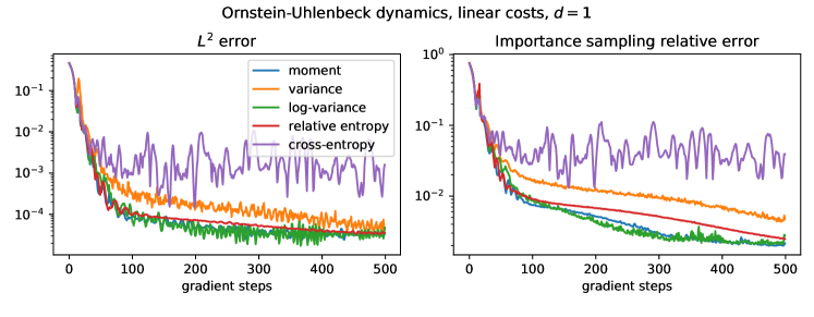
Figure 1: Performance of the algorithm using five different loss functions according to the metrics introduced in Section 6.1 as a function of the iteration step.

Figure 2 shows the algorithm’s performance in a high-dimensional case, $d=40$, where we now choose $N=500$ as the batch size, $\eta=0.001$ as the learning rate, $\Delta t=0.01$ as the time step, and as before rely on a DenseNet with two hidden layers. We observe that relative entropy loss and log-variance loss perform best, and that the moment and cross-entropy losses converge at a significantly slower rate. The variance loss is numerically unstable and hence not represented in Figure 2. We encounter similar problems in the subsequent experiments and thus do not consider the variance loss in what follows. In Figure 3 we plot some of the components of the $40$-dimensional approximated optimal control vector field as well as the analytic solution $u_{\mathrm{ref}}^{*}(x,t)$ for a fixed value of $x$ and varying time $t$, showcasing the inferiority of the approximation obtained using the cross-entropy loss. The comparatively poor performance of the cross-entropy and the variance losses can be attributed to their non-robustness with respect to tensorisations, see Section 5.2. To further illustrate these results, Figure 4 displays the relative error associated to the loss estimators computed from $N=15\cdot 10^{6}$ samples in different dimensions. The dimensional dependence agrees with what is expected from Proposition 5.7, but we note that our numerical experiment goes beyond the product case.

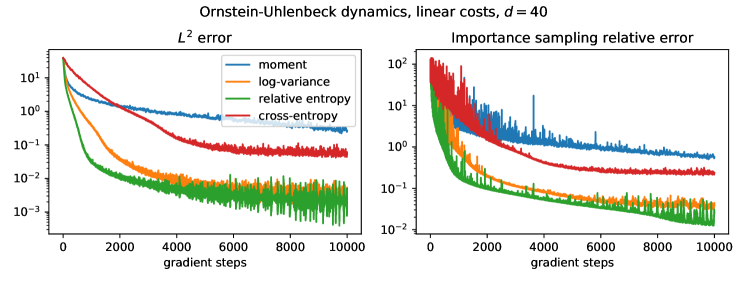
Figure 2: Performance of the algorithm using four different loss functions in a high-dimensional setting.

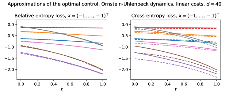
Figure 3: Approximation $u$ (dashed lines) and reference solution $u^{*}_{\text{ref}}$ (straight lines) for the optimal control obtained using the relative entropy and cross-entropy losses, respectively. $7$ out of the $40$ components of $u$ and $u^{*}_{\text{ref}}$ are plotted.

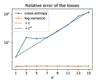
Figure 4: Relative error of the log-variance and cross-entropy losses depending on the dimension.

Lastly, let us investigate the effect of the additional parameter $y_{0}$ in the moment loss. For a first experiment, we initialise $y_{0}$ with either the naive choice $y_{0}^{(1)}=0$, or $y_{0}^{(2)}=10$, a starting value which differs considerably from $-\log\mathcal{Z}$ or the optimal choice $y_{0}^{(3)}=-\log\mathcal{Z}\approx-5.87$. Let us insist that in practical scenarios the value of $-\log\mathcal{Z}$ is usually not known. Additionally, we contrast using Adam and SGD as an optimisation routine – in both cases we choose $N=200$, $\eta=0.01$, $\Delta t=0.01$, and the same DenseNet architecture as in the previous experiments.

Figure 5 shows that the initialisation of $y_{0}$ can have a significant impact on the convergence speed. Indeed, with the initialisation $y_{0}=-\log\mathcal{Z}$, the moment and log-variance losses perform very similarly, in accordance with Proposition 4.6. In contrast, choosing the initial value $y_{0}$ such that the discrepancy $|y_{0}+\log\mathcal{Z}|$ is large incurs a much slower convergence.

Comparing the two plots in Figure 5 shows that the Adam optimiser achieves a much faster convergence overall in comparison to SGD. Moreover, the difference in performance between $y_{0}$-initialisations is more pronounced when the Adam optimiser is used. The observations in these experiments are in agreement with those in [23].

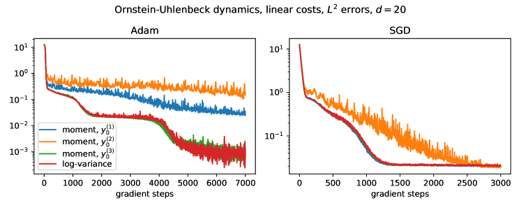
Figure 5: Performance of the algorithm with the moment loss and different initialisations for $y_{0}$, using Adam and SGD.

6.3 Ornstein-Uhlenbeck dynamics with quadratic costs

We consider the Ornstein-Uhlenbeck process described by (99) with quadratic running and terminal costs, i.e. $f(x,s)=x^{\top}Px$ and $g(x)=x^{\top}Rx$, with $P,R\in\operatorname*{\mathbb{R}}^{d\times d}$. This setting is known as the linear quadratic Gaussian control problem [119]. The optimal control is given by [119, Section 6.5]

$$u^{*}(x,t) =-2B_{t}^{\top}F_{t}x,$$ (101)

where the matrices $F_{t}$ fulfill the matrix Riccati equation

$$\frac{\mathrm{d}}{\mathrm{d}t}F_{t}+A^{\top}_{t}F_{t}+F_{t}A_{t}-2F_{t}B_{t}B_{t}^{\top}F_{t}+P=0,\qquad F_{T}=R.$$ (102)

In this example, we demonstrate an approach leveraging a priori knowledge about the structure of the solution. Motivated by (101), we consider the linear ansatz functions

$$u(x,t_{n})=\Xi_{n}x,$$ (103)

where the entries of the matrices $\Xi_{n}\in\operatorname*{\mathbb{R}}^{d\times d}$, $n=0,\ldots,K-1$ represent the parameters to be learnt. The matrices $A$ and $B$ are chosen as in Subsection 6.2 and we set $P=\frac{1}{2}I_{d\ \times d}$, $R=I_{d\times d}$ and $T=0.5$. Figure 6 shows the performance using Adam with learning rate $\eta=0.001$ and SGD with learning rate $\eta=0.01$, respectively. The relative entropy losses converges fastest, followed by the log-variance loss. The convergence of the cross-entropy loss is significantly slower, in particular in the SGD case. We also note that the cross-entropy loss diverges if larger learning rates are used. These findings are in line with the results from Proposition 5.7. When SGD is used, the moment loss experiences fluctuations in later gradient steps. This can be explained by the fact that the moment loss is robust at $u^{*}$ only if $y_{0}=-\log\mathcal{Z}$ is satisfied exactly (see Proposition 4.6).

Let us illustrate the potential benefit of sampling $X_{0}$ from a predescribed density (see Remark 2.5), here $X_{0}\sim\mathcal{N}(0,I_{d\times d})$. The overall convergence is hardly affected and the $L^{2}$ error dynamics agrees qualitatively with the one shown in Figure 6. However, the approximation is more accurate at initial time $t=0$, see Figure 7. This phenomenon appears to be particularly pronounced in this example, as independent ansatz functions are used at each time step.

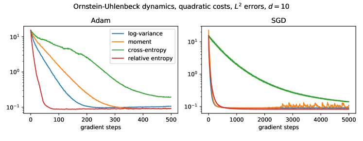
Figure 6: Performance of the losses for the Ornstein-Uhlenbeck process with quadratic costs, using Adam and SGD.

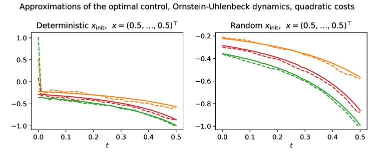
Figure 7: Approximation and reference solution of the optimal control with either deterministic or random initialisations of $x_{\text{init}}$. Three components of $u$ and $u_{\text{ref}}^{*}$ are plotted.

6.4 Metastable dynamics in low and high dimensions

We now come back to the double well potential from Example 2.1 and consider the SDE

$$\mathrm{d}X_{s}=-\nabla\Psi(X_{s})\,\mathrm{d}s+B\,\mathrm{d}W_{s},\quad X_{0}=x_{\text{init}},$$ (104)

where $B\in\operatorname*{\mathbb{R}}^{d\times d}$ is the diffusion coefficient, $\Psi(x)=\sum_{i=1}^{d}\kappa_{i}(x_{i}^{2}-1)^{2}$ is the potential (with $\kappa_{i}>0$ being a set of parameters) and $x_{\text{init}}=(-1,\dots,-1)^{\top}$ is the initial condition. We consider zero running costs, $f=0$, terminal costs $g(x)=\sum_{i=1}^{d}\nu_{i}(x_{i}-1)^{2}$, where $\nu_{i}>0$, and a terminal time $T=1$. Recall from Example 2.1 that choosing higher values for $\kappa_{i}$ and $\nu_{i}$ accentuates the metastable features, making sample-based estimation of $\operatorname*{\mathbb{E}}\left[\exp(-g(X_{T}))\right]$ more challenging. For an illustration, Figure 8 shows the potential $\Psi$ and the weight at final time $e^{-g}$ (see (15)), for different values of $\nu$ and $\kappa$, in dimension $d=1$ and for $B=1$. We furthermore plot the ‘optimally tilted potentials’ $\Psi^{*}=\Psi+BB^{\top}V$, noting that $-\nabla\Psi^{*}=-\nabla\Psi+Bu^{*}$. Finally, the right-hand side shows the gradients $\nabla u^{*}$ at initial time $t=0$.

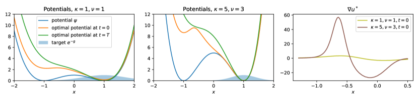
Figure 8: The double well potential and the weight $e^{-g}$, for different values of $\kappa$ and $\nu$ as well as optimal controls (inducing ‘tilted potentials’) and their gradients.

For an experiment, let us first consider the one-dimensional case, choosing $B=1$, $\kappa=5$ and $\nu=3$. In this setting the relative error associated to the standard Monte Carlo estimator, i.e. the estimator version of (97), which we denote by $\widehat{\delta}$, is roughly $\widehat{\delta}(0)=63.86$ for a batch size of $N=10^{7}$ trajectories, from which only about $2\cdot 10^{3}$ (i.e. 0.02%) cross the barrier. Given that $e^{-g}$ is supported mostly in the right well, the optimal control $u^{*}$ steers the dynamics across the barrier. Using an approximation of $u^{*}$ obtained by a finite difference scheme, we achieve a relative error of $\widehat{\delta}(u^{*})=1.94$ (the theoretical optimum being zero, according to Theorem 2.2) and a crossing ratio of approximately 87.28%.

To run IDO-based algorithms, we use the standard feed-forward neural network (see Definition 6.1) with the activation function $\varrho=\tanh$ and choose $\Delta t=0.005$, $\eta=0.05$. We try batch sizes of $N=50$ and $N=1000$ and plot the training progress in Figures 9 and 10, respectively. In Figure 11 we display the approximation obtained using the log-variance loss and compare with the reference solution $u^{*}_{\mathrm{ref}}$.

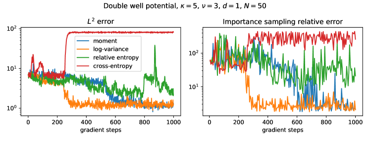
Figure 9: Training iterations for the one-dimensional metastable double well example for a small batch size.

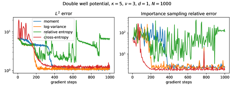
Figure 10: Training iterations for the one-dimensional metastable double well example for a large batch size.

It can be observed that the log-variance and moment losses perform well with both batch sizes, with the log-variance loss however achieving a satisfactory approximation with fewer gradient steps. The cross-entropy loss appears to work well only if the batch size is sufficiently large. We attribute this observation to the non-robustness at $u^{*}$ (see Proposition 5.3) and, tentatively, to the exponential factor appearing in (48b), see Remark 3.8.

The optimisation using the relative entropy loss is frustrated by instabilities in the vicinity of the solution $u^{*}$. In order to further investigate this aspect we numerically compute the variances of the gradients and the associated relative errors with respect to the mean, using $50$ realisations at each gradient step. Figure 12 shows the averages of the relative errors and variances over weights in the network, confirming that the gradients associated to the log-variance loss have significantly lower variances. This phenomenon is in accordance with Proposition 5.3 (in particular noting that $|\nabla u^{*}|^{2}$ is expected to be rather large in a metastable setting, see Figure 8) and explains the unsatisfactory behaviour of the relative entropy loss observed in Figures 9 and 10.

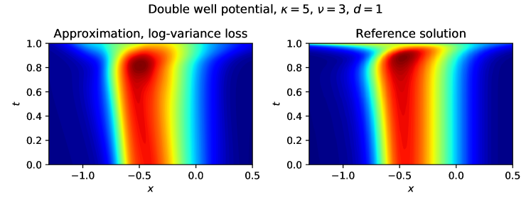
Figure 11: Approximation and reference solution for the double well control problem in $d=1$.

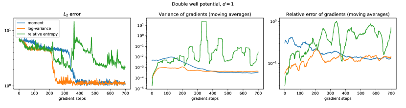
Figure 12: We display the $L_{2}$ error pertaining to the one-dimensional double well experiment, along with the estimated averages of the variances and relative errors of the gradients along the training iterations for different losses.

Let us now consider the multidimensional setting, namely $d=10$, where the dynamics exhibits ‘highly’ metastable characteristics in 3 dimensions and ‘weakly’ metastable characteristics in the remaining 7 dimensions. To be precise, we set $\kappa_{i}=5$, $\nu_{i}=3$ for $i\in\{1,2,3\}$ and $\kappa_{i}=1$, $\nu_{i}=1$ for $i\in\{4,\dots,10\}$. Moreover, we choose the diffusion coefficient to be $B=I_{d\times d}$ and conduct the experiment with a batch size of $N=500$.

In Figure 13 we see that only the log-variance loss achieves a reasonable approximation. Interestingly, the training progresses in stages, successively overcoming the potential barriers in the highly metastable directions. On the right-hand side we display the components of the approximated optimal control associated to one highly and one weakly metastable direction, for fixed $t=0$. We observe that the approximation is fairly accurate, and that comparatively large control forces are needed to push the dynamics over the highly metastable potential barrier.

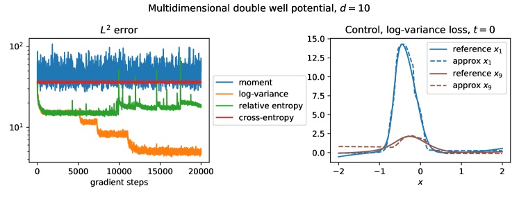
Figure 13: Training iterations for the multidimensional metastable double well along with the approximated solution using the log-variance loss, from which we plot two components.

7 Conclusion and outlook

Motivated by the observation that optimal control of diffusions can be phrased in a number of different ways, we have provided a unifying framework based on divergences between path measures, encompassing various existing numerical methods in the class of IDO algorithms. In particular, we have shown that the novel log-variance divergences are closely connected to forward-backward SDEs. We have furthermore shown a fundamental equivalence between approaches based on the $\mathrm{KL}$-divergence and the log-variance divergences.

Turning to the variance of Monte Carlo gradient estimators, we have defined and studied two notions of stability – robustness under tensorisation and robustness at the optimal control solution. Of the losses and estimators under consideration, only the log-variance loss is stable in both senses, often resulting in superior numerical performance. The consequences of robustness and non-robustness as defined have been exemplified by extensive numerical experiments.

The results presented in this paper can be extended in various directions. First, it would be interesting to consider other divergences on path space and construct and study the ensuing algorithms. In this respect, we may also mention the development of more elaborate schemes to update the control for the forward dynamics. Second, one may attempt to generalise the current framework to other types of control problems and PDEs (for instance to elliptic PDEs and hitting time problems as considered in [55, 56, 59, 60], or to the Schrödinger problem as discussed in [104]). Deeper understanding of the design of IDO algorithms could be achieved by extending our stability analysis beyond the product case and for controls that differ greatly from the optimal one. In particular, advances in this direction might help to develop more sophisticated variance reduction techniques. Finally, we envision applications of the log-variance divergences in other settings.

Acknowledgements. This research has been funded by Deutsche Forschungsgemeinschaft (DFG) through the grant CRC 1114 ‘Scaling Cascades in Complex Systems’ (projects A02 and A05, project number 235221301). We would like to thank Carsten Hartmann and Wei Zhang for many very useful discussions. We thank the referees for their useful comments and suggestions that have led to various improvements in the presentation of this paper.

Appendix A Appendix

A.1 Proofs for Section 3.1

The Radon-Nikodym derivatives appearing in the divergences defined in Section 3.1 can be computed explicitly:

Lemma A.1.

For $u\in\mathcal{U}$, the measures $\mathbb{P}$ and $\mathbb{P}^{u}$ are equivalent. Moreover, the Radon-Nikodym derivative satisfies

$$\frac{\mathrm{d}\mathbb{P}^{u}}{\mathrm{d}\mathbb{P}}(X)=\exp\left(\int_{0}^{T}\left(u^{\top}\sigma^{-1}\right)(X_{s},s)\cdot\mathrm{d}X_{s}-\int_{0}^{T}(\sigma^{-1}b\cdot u)(X_{s},s)\,\mathrm{d}s-\frac{1}{2}\int_{0}^{T}|u(X_{s},s)|^{2}\,\mathrm{d}s\right)$$ (105)

Proof.

The fact that the two measures are equivalent follows from the linear growth assumption on $u$ (see (6)), combining Beneš’ theorem with Girsanov’s theorem, see [118, Proposition 2.2.1 and Theorem 2.1.1]. According to a slight generalisation of [118, Theorem 2.4.2], we have

$$\frac{\mathrm{d}\mathbb{P}}{\mathrm{d}\mathbb{P}_{\mathrm{W}}}(X)=\exp\left(\int_{0}^{T}(b(X_{s},s)\cdot\sigma^{-2}(X_{s},s)\,\mathrm{d}X_{s}-\frac{1}{2}\int_{0}^{T}(b\cdot\sigma^{-2}b)(X_{s},s)\,\mathrm{d}s\right),$$ (106)

and

$$\frac{\mathrm{d}\mathbb{P}^{u}}{\mathrm{d}\mathbb{P}_{\mathrm{W}}}(X)=\exp\left(\int_{0}^{T}(b+\sigma u)(X_{s},s)\cdot\sigma^{-2}(X_{s},s)\,\mathrm{d}X_{s}-\frac{1}{2}\int_{0}^{T}\left((b+\sigma u)\cdot\sigma^{-2}(b+\sigma u)\right)(X_{s},s)\,\mathrm{d}s\right),$$ (107)

where $\mathbb{P}_{\mathrm{W}}$ denotes the measure on $\mathcal{C}$ induced by

$$\mathrm{d}X_{s}=\sigma(X_{s},s)\,\mathrm{d}W_{s},\qquad X_{0}=x_{\mathrm{init}}.$$ (108)

Using

$$\frac{\mathrm{d}\mathbb{P}^{u}}{\mathrm{d}\mathbb{P}}(X)=\frac{\mathrm{d}\mathbb{P}^{u}}{\mathrm{d}\mathbb{P}_{\mathrm{W}}}\frac{\mathrm{d}\mathbb{P}_{\mathrm{W}}}{\mathrm{d}\mathbb{P}}(X),$$ (109)

and inserting (106) and (107), we obtain the desired result. ∎

Proof of Proposition 3.5.

Using (15) and (105) (or arguing as in the proof of Theorem 2.2) we compute

$$\mathcal{L}_{\text{RE}}(u) ={\operatorname*{\mathbb{E}}}_{\mathbb{P}^{u}}\left[\log\frac{\mathrm{d}\mathbb{P}^{u}}{\mathrm{d}\mathbb{Q}}\right]={\operatorname*{\mathbb{E}}}_{\mathbb{P}^{u}}\left[\log\left(\frac{\mathrm{d}\mathbb{P}^{u}}{\mathrm{d}\mathbb{P}}\frac{\mathrm{d}\mathbb{P}}{\mathrm{d}\mathbb{Q}}\right)\right]$$ (110a)

$$={\operatorname*{\mathbb{E}}}\left[\int_{0}^{T}u(X_{s}^{u},s)\cdot\,\mathrm{d}W_{s}+\frac{1}{2}\int_{0}^{T}|u(X^{u}_{s},s)|^{2}\,\mathrm{d}s+\int_{0}^{T}f(X^{u}_{s},s)\mathrm{d}s+g(X^{u}_{T})\right]+\log\mathcal{Z}$$ (110b)

$$={\operatorname*{\mathbb{E}}}\left[\frac{1}{2}\int_{0}^{T}|u(X^{u}_{s},s)|^{2}\,\mathrm{d}s+\int_{0}^{T}f(X^{u}_{s},s)\mathrm{d}s+g(X^{u}_{T})\right]+\log\mathcal{Z}.$$ (110c)

∎

Proof of Proposition 3.7.

Similarly, we compute

$$\mathcal{L}_{\text{CE}}(u) ={\operatorname*{\mathbb{E}}}_{\mathbb{Q}}\left[\log\frac{\mathrm{d}\mathbb{Q}}{\mathrm{d}\mathbb{P}^{u}}\right]={\operatorname*{\mathbb{E}}}_{\mathbb{P}^{v}}\left[\log\left(\frac{\mathrm{d}\mathbb{Q}}{\mathrm{d}\mathbb{P}}\frac{\mathrm{d}\mathbb{P}}{\mathrm{d}\mathbb{P}^{u}}\right)\frac{\mathrm{d}\mathbb{Q}}{\mathrm{d}\mathbb{P}}\frac{\mathrm{d}\mathbb{P}}{\mathrm{d}\mathbb{P}^{v}}\right]$$ (111a)

$$\begin{split}&={\operatorname*{\mathbb{E}}}\Bigg{[}\left(\frac{1}{2}\int_{0}^{T}|u(X^{v}_{s},s)|^{2}\,\mathrm{d}s-\int_{0}^{T}(u\cdot v)(X^{v},s)\,\mathrm{d}s-\int_{0}^{T}u(X_{s}^{v},s)\cdot\,\mathrm{d}W_{s}-\mathcal{W}(X^{v})-\log\mathcal{Z}\right)\\ &\qquad\qquad\frac{1}{\mathcal{Z}}\exp\left(-\mathcal{W}(X^{v})-\int_{0}^{T}v(X_{s}^{v},s)\cdot\,\mathrm{d}W_{s}-\frac{1}{2}\int_{0}^{T}|v(X^{v}_{s},s)|^{2}\,\mathrm{d}s\right)\Bigg{]}\end{split}$$ (111b)

$$\begin{split}&=\frac{1}{\mathcal{Z}}{\operatorname*{\mathbb{E}}}\Bigg{[}\left(\frac{1}{2}\int_{0}^{T}|u(X^{v}_{s},s)|^{2}\,\mathrm{d}s-\int_{0}^{T}(u\cdot v)(X_{s}^{v},s)\mathrm{d}s-\int_{0}^{T}u(X_{s}^{v},s)\cdot\,\mathrm{d}W_{s}\right)\\ &\qquad\qquad\exp\left(-\int_{0}^{T}v(X_{s}^{v},s)\cdot\,\mathrm{d}W_{s}-\frac{1}{2}\int_{0}^{T}|v(X^{v}_{s},s)|^{2}\,\mathrm{d}s-\mathcal{W}(X^{v})\right)\Bigg{]}+C\end{split},$$ (111c)

where $C\in\operatorname*{\mathbb{R}}$ does not depend on $u$. ∎

Proof of Proposition 3.10.

With $\widetilde{Y}_{T}^{u,v}$ defined as in (51), we compute for the variance loss

$$\mathcal{L}_{\text{Var}_{v}}(u) ={\operatorname*{\operatorname{Var}}}_{\mathbb{P}^{v}}\left(\frac{\mathrm{d}\mathbb{Q}}{\mathrm{d}\mathbb{P}^{u}}\right)={\operatorname*{\operatorname{Var}}}_{\mathbb{P}^{v}}\left(\frac{\mathrm{d}\mathbb{Q}}{\mathrm{d}\mathbb{P}}\frac{\mathrm{d}\mathbb{P}}{\mathrm{d}\mathbb{P}^{u}}\right)=\frac{1}{\mathcal{Z}^{2}}\,{\operatorname*{\operatorname{Var}}}_{\mathbb{P}^{v}}\left(e^{\widetilde{Y}_{T}^{u,v}-g(X_{T}^{v})}\right).$$ (112)

Similarly, the log-variance loss equals

$$\mathcal{L}^{\log}_{\text{Var}_{v}}(u) ={\operatorname*{\operatorname{Var}}}_{\mathbb{P}^{v}}\left(\log\frac{\mathrm{d}\mathbb{Q}}{\mathrm{d}\mathbb{P}^{u}}\right)={\operatorname*{\operatorname{Var}}}_{\mathbb{P}^{v}}\left(\log\left(\frac{\mathrm{d}\mathbb{P}}{\mathrm{d}\mathbb{P}^{u}}\frac{\mathrm{d}\mathbb{Q}}{\mathrm{d}\mathbb{P}}\right)\right)={\operatorname*{\operatorname{Var}}}_{\mathbb{P}^{v}}\left(\widetilde{Y}_{T}^{u,v}-g(X_{T}^{v})-\log\mathcal{Z}\right)$$ (113a)

$$={\operatorname*{\operatorname{Var}}}_{\mathbb{P}^{v}}\left(\widetilde{Y}_{T}^{u,v}-g(X_{T}^{v})\right).$$ (113b)

∎

A.2 Proofs for Section 4

Proof of Proposition 4.3.

For $\varepsilon\in\mathbb{R}$ and $\phi\in C_{b}^{1}(\mathbb{R}^{d}\times[0,T];\mathbb{R}^{d})$, let us define the change of measure

$$\Lambda_{T}(\varepsilon,\phi)=\exp\left(-\varepsilon\int_{0}^{T}\phi(X^{u}_{s},s)\cdot\mathrm{d}W_{s}-\frac{\varepsilon^{2}}{2}\int_{0}^{T}|\phi(X^{u}_{s},s)|^{2}\,\mathrm{d}s\right),\qquad\frac{\mathrm{d}\widetilde{\Theta}}{\mathrm{d}\Theta}=\Lambda_{T}(\varepsilon,\phi).$$ (114)

According to Girsanov’s theorem, the process $(\widetilde{W}_{s})_{0\leq s\leq T}$, defined as

$$\widetilde{W}_{t}=W_{t}+\varepsilon\int_{0}^{t}\phi(X^{u}_{s},s)\,\mathrm{d}s,$$ (115)

is a Brownian motion under $\widetilde{\Theta}$. We therefore obtain

$$\mathcal{L}_{\mathrm{RE}}(u+\varepsilon\phi)=\mathbb{E}\left[\left(\frac{1}{2}\int_{0}^{T}|(u+\varepsilon\phi)(X_{s}^{u},s)|^{2}\,\mathrm{d}s+\int_{0}^{T}f(X_{s}^{u},s)\,\mathrm{d}s+g(X_{T}^{u})\right)\Lambda^{-1}_{T}(\varepsilon,\phi)\right]+\log\mathcal{Z}.$$ (116)

Using dominated convergence, we can interchange derivatives and integrals (for technical details, we refer to [83]) and compute

$$\frac{\mathrm{d}}{\mathrm{d}\varepsilon}\Big{|}_{\varepsilon=0}\mathcal{L}_{\operatorname*{\mathrm{RE}}}(u+\varepsilon\phi) =\mathbb{E}\left[\int_{0}^{T}(u\cdot\phi)(X_{s}^{u},s)\,\mathrm{d}s+\left(\frac{1}{2}\int_{0}^{T}|u(X_{s}^{u},s)|^{2}\,\mathrm{d}s+\int_{0}^{T}f(X_{s}^{u},s)\,\mathrm{d}s+g(X_{T}^{u})\right)\int_{0}^{T}\phi(X_{s}^{u},s)\cdot\mathrm{d}W_{s}\right]$$ (117a)

$$={\operatorname*{\mathbb{E}}}\left[\left(g(X_{T}^{u})-\widetilde{Y}_{T}^{u,u}\right)\int_{0}^{T}\phi(X_{s}^{u},s)\cdot\mathrm{d}W_{s}\right],$$ (117)

where we have used Itô’s isometry,

$$\mathbb{E}\left[\int_{0}^{T}\phi(X_{s}^{u},s)\cdot\mathrm{d}W_{s}\int_{0}^{T}u(X_{s}^{u},s)\cdot\mathrm{d}W_{s}\right]=\mathbb{E}\left[\int_{0}^{T}(u\cdot\phi)(X_{s}^{u},s)\,\mathrm{d}s\right].$$ (118)

Turning to the log-variance loss, we see that

$$\frac{\mathrm{d}}{\mathrm{d}\varepsilon}\Big{|}_{\varepsilon=0}\mathcal{L}^{\log}_{\operatorname*{\operatorname{Var}}_{v}}(u+\varepsilon\phi)=\frac{\mathrm{d}}{\mathrm{d}\varepsilon}\Big{|}_{\varepsilon=0}\left(\mathbb{E}\left[\left(\widetilde{Y}_{T}^{u+\varepsilon\phi,v}-g(X_{T}^{v})\right)^{2}\right]-\mathbb{E}\left[\left(\widetilde{Y}_{T}^{u+\varepsilon\phi,v}-g(X_{T}^{v})\right)\right]^{2}\right)$$ (119a)

$$= 2\,\mathbb{E}\left[\left(\widetilde{Y}_{T}^{u,v}-g(X_{T}^{v})\right)\frac{\mathrm{d}}{\mathrm{d}\varepsilon}\Big{|}_{\varepsilon=0}\widetilde{Y}_{T}^{u+\varepsilon\phi,v}\right]-2\,\mathbb{E}\left[\left(\widetilde{Y}_{T}^{u,v}-g(X_{T}^{v})\right)\right]\mathbb{E}\left[\frac{\mathrm{d}}{\mathrm{d}\varepsilon}\Big{|}_{\varepsilon=0}\widetilde{Y}_{T}^{u+\varepsilon\phi,v}\right],$$ (119b)

where

$$\frac{\mathrm{d}}{\mathrm{d}\varepsilon}\Big{|}_{\varepsilon=0}\widetilde{Y}_{T}^{u+\varepsilon\phi,v}=\int_{0}^{T}(\phi\cdot(u-v))(X_{s}^{v},s)\,\mathrm{d}s-\int_{0}^{T}\phi(X_{s}^{v},s)\cdot\mathrm{d}W_{s}.$$ (120)

Setting $v=u$, we obtain

$$\left(\frac{\mathrm{d}}{\mathrm{d}\varepsilon}\Big{|}_{\varepsilon=0}\mathcal{L}^{\log}_{\operatorname*{\operatorname{Var}}_{v}}(u+\varepsilon\phi)\right)\Big{|}_{v=u}=2\,{\operatorname*{\mathbb{E}}}\left[\left(g(X_{T}^{u})-\widetilde{Y}_{T}^{u,u}\right)\int_{0}^{T}\phi(X_{s}^{u},s)\cdot\mathrm{d}W_{s}\right],$$ (121)

from which the result follows by comparison with (117). ∎

Proof of Proposition 4.6.

We compute

$$\frac{\mathrm{d}}{\mathrm{d}\varepsilon}\Big{|}_{\varepsilon=0}\mathcal{L}_{\text{moment}_{v}}(u+\varepsilon\phi)=2\,\mathbb{E}\left[\left(\widetilde{Y}_{T}^{u,v}+y_{0}-g(X_{T}^{v})\right)\left(\int_{0}^{T}(\phi\cdot(u-v))(X_{s}^{v},s)\,\mathrm{d}s-\int_{0}^{T}\phi(X_{s}^{v},s)\cdot\mathrm{d}W_{s}\right)\right].$$ (122)

Setting $v=u$ and using that ${\operatorname*{\mathbb{E}}}\left[y_{0}\int_{0}^{T}\phi(X_{s}^{v},s)\cdot\mathrm{d}W_{s}\right]=0$, the first statement follows by comparison with (69). The second statement follows from

$$\left(\frac{\delta}{\delta u}\mathcal{L}_{\mathrm{moment}_{v}}(u,y_{0};\phi)\right)\Big{|}_{u=u^{*}}=2\,\mathbb{E}\left[\left(y_{0}+\log\mathcal{Z}\right)\left(\int_{0}^{T}(\phi\cdot(u^{*}-v))(X_{s}^{v},s)\,\mathrm{d}s\right)\right],$$ (123)

where we have used the fact that $\widetilde{Y}_{T}^{u^{*},v}-g(X_{T}^{v})=\log\mathcal{Z}$, almost surely. ∎

A.3 Proofs for Section 5

Proof of Proposition 5.3.

1.) We compute

$$\frac{\delta}{\delta u}\Big{|}_{u=u^{*}}\widehat{\mathcal{L}}^{(N)}_{\operatorname*{\operatorname{Var}}_{v}}(u;\phi)=2\,\Bigg{(}\frac{1}{N}\sum_{i=1}^{N}\left[\exp\left(2\left(\widetilde{Y}_{T}^{u^{*},v,(i)}-g\left(X_{T}^{v,(i)}\right)\right)\right)\frac{\delta\widetilde{Y}_{T}^{u,v,(i)}}{\delta u}(u^{*};\phi)\right]$$ (124a)

$$-\frac{1}{N}\sum_{i=1}^{N}\left[\exp\left(\widetilde{Y}_{T}^{u^{*},v,(i)}-g\left(X_{T}^{v,(i)}\right)\right)\frac{\delta\widetilde{Y}_{T}^{u,v,(i)}}{\delta u}(u^{*};\phi)\right]\frac{1}{N}\sum_{i=1}^{N}\left[\exp\left(\widetilde{Y}_{T}^{u^{*},v,(i)}-g\left(X_{T}^{v,(i)}\right)\right)\right]\Bigg{)},$$ (124b)

where $\frac{\delta\widetilde{Y}_{T}^{u,v,(i)}}{\delta u}(u;\phi)$ is given in (82). As in the proof for the log-variance estimator, the quantity

$$\exp\left(\widetilde{Y}_{T}^{u^{*},v,(i)}-g\left(X_{T}^{v,(i)}\right)\right)$$ (125)

is almost surely constant and thus the statement follows.

2.) Similarly to the computations involved in 1.) we have

$$\frac{\delta}{\delta u}\Big{|}_{u=u^{*}}\widehat{\mathcal{L}}^{(N)}_{\operatorname{moment}_{v}}(u,y_{0};\phi)=\frac{2}{N}\sum_{i=1}^{N}\left(\widetilde{Y}_{T}^{u^{*},v,(i)}+y_{0}-g\left(X_{T}^{u^{*},(i)}\right)\right)\frac{\delta\widetilde{Y}_{T}^{u,v,(i)}}{\delta u}(u^{*};\phi)$$ (126a)

$$=\frac{2}{N}\left(-\log\mathcal{Z}+y_{0}\right)\sum_{i=1}^{N}\left(\int_{0}^{T}\phi(X_{s}^{v,(i)},s)\cdot\mathrm{d}W^{(i)}_{s}-\int_{0}^{T}\left(\phi\cdot(u^{*}-v)\right)(X_{s}^{v,(i)},s)\,\mathrm{d}s\right),$$ (126b)

where we have used the fact that $\widetilde{Y}_{T}^{u^{*},v,(i)}-g\left(X_{T}^{u^{*},(i)}\right)=-\log\mathcal{Z}$ according to (24) and (55b). The variance of this expression equals

$$\frac{4}{N}\left(\log\mathcal{Z}-y_{0}\right)^{2}\operatorname*{\mathbb{E}}\left[\left(\int_{0}^{T}\phi(X_{s}^{v,(i)},s)\cdot\mathrm{d}W^{(i)}_{s}-\int_{0}^{T}\left(\phi\cdot(u^{*}-v)\right)(X_{s}^{v,(i)},s)\,\mathrm{d}s\right)^{2}\right],$$ (127)

implying the claim.

3.) Let $\phi\in C_{b}^{1}(\mathbb{R}^{d}\times[0,T];\mathbb{R}^{d})$ and $\varepsilon\in\mathbb{R}$. As usual, we denote by $(X_{s}^{u^{*}+\varepsilon\phi})_{0\leq s\leq T}$ the unique strong solution to (5), with $u$ replaced by $u^{*}+\varepsilon\phi$. By a slight modification of [81, Theorems 3.1 and 3.3] detailed, for instance, in [93, Section 10.2.2], $X_{s}^{u^{*}+\varepsilon\phi}$ is almost surely differentiable as a function of $\varepsilon$. Furthermore, $\frac{\mathrm{d}X_{s}^{u^{*}+\varepsilon\phi}}{\mathrm{d}\varepsilon}\Big{|}_{\varepsilon=0}=:A_{s}$ satisfies the SDE (80). We calculate

$$\frac{\mathrm{d}}{\mathrm{d}\varepsilon}\Big{|}_{\varepsilon=0}\left[\frac{1}{2}\int_{0}^{T}|u^{*}+\varepsilon\phi|^{2}(X_{s}^{u^{*}+\varepsilon\phi},s)\,\mathrm{d}s+\int_{0}^{T}f(X_{s}^{u^{*}+\varepsilon\phi},s)\,\mathrm{d}s+g(X_{T}^{u^{*}+\varepsilon\phi})\right]$$ (128a)

$$=\int_{0}^{T}(u^{*}\cdot\phi)(X_{s}^{u^{*}},s)\,\mathrm{d}s+\frac{1}{2}\int_{0}^{T}(\nabla|u^{*}|^{2})(X_{s}^{u^{*}},s)\cdot A_{s}\,\mathrm{d}s+\int_{0}^{T}\nabla f(X_{s}^{u^{*}},s)\cdot A_{s}\,\mathrm{d}s+\nabla g(X_{T}^{u^{*}})\cdot A_{T}.$$ (128b)

From (11b) and using integration by parts, we see that the last term in (128b) satisfies

$$(\nabla g)(X_{T}^{u^{*}})\cdot A_{T}=\nabla V(X_{T}^{u^{*}},T)\cdot A_{T}=\int_{0}^{T}\nabla V(X^{u^{*}}_{s},s)\cdot\mathrm{d}A_{s}+\int_{0}^{T}A_{s}\cdot\mathrm{d}(\nabla V(X^{u^{*}}_{s},s))+\left\langle A_{\cdot},\nabla V(X_{\cdot}^{u^{*}},\cdot)\right\rangle_{T}.$$ (129)

Next, we employ Itô’s formula and Einstein’s summation convention to compute

$$\mathrm{d}(\partial_{x_{i}}V(X^{u^{*}}_{s},s))=$$ (130a)

$$=\left[\partial_{x_{i}}\partial_{s}V+(\partial_{x_{i}}\partial_{x_{j}}V)(b+\sigma u^{*})_{j}+\frac{1}{2}(\partial_{x_{i}}\partial_{x_{j}}\partial_{x_{k}}V)\sigma_{jl}\sigma_{kl}\right](X_{s}^{u^{*}},s)\,\mathrm{d}s+\left[(\partial_{x_{i}}\partial_{x_{j}}V)\sigma_{jk}\right](X_{s}^{u^{*}},s)\,\mathrm{d}W_{s}^{k}$$ (130b)

$$=\partial_{x_{i}}\left[\partial_{s}V+LV-\frac{1}{2}(\partial_{x_{j}}V)\sigma_{jk}\sigma_{lk}(\partial_{x_{l}}V)\right](X_{s}^{u^{*}},s)\,\mathrm{d}s+\left[(\partial_{x_{i}}\partial_{x_{j}}V)\sigma_{jk}\right](X_{s}^{u^{*}},s)\,\mathrm{d}W_{s}^{k}$$ (130c)

$$+\left[\frac{1}{2}\left((\partial_{x_{j}}V)(\partial_{x_{l}}V)-\partial_{x_{j}}\partial_{x_{l}}V\right)\partial_{x_{i}}(\sigma_{jk}\sigma_{lk})-(\partial_{x_{j}}V)\partial_{x_{i}}b_{j}\right](X_{s}^{u^{*}},s)\,\mathrm{d}s$$ (130d)

$$=\left[\frac{1}{2}\left((\partial_{x_{j}}V)(\partial_{x_{l}}V)-\partial_{x_{j}}\partial_{x_{l}}V\right)\partial_{x_{i}}(\sigma_{jk}\sigma_{lk})-(\partial_{x_{j}}V)\partial_{x_{i}}b_{j}-\partial_{x_{i}}f\right](X_{s}^{u^{*}},s)\,\mathrm{d}s$$ (130e)

$$+\left[(\partial_{x_{i}}\partial_{x_{j}}V)\sigma_{jk}\right](X_{s}^{u^{*}},s)\,\mathrm{d}W_{s}^{k},$$ (130f)

where we used (37) from the second to the third line and (11) to manipulate the first term in the third line. Using (80) and (130), we see that the quadratic variation process satisfies

$$\left\langle A_{\cdot},\nabla V(X_{\cdot}^{u^{*}},\cdot)\right\rangle_{T}=\frac{1}{2}\int_{0}^{T}A_{j}\left[\partial_{x_{j}}(\sigma_{ik}\sigma_{lk})(\partial_{x_{i}}\partial_{x_{l}}V)\right](X_{s}^{u^{*}},s)\,\mathrm{d}s.$$ (131)

Combining (80), (129), (130) and (131), it follows that (128) equals

$$\int_{0}^{T}\left[A_{j}(\partial_{x_{i}}V)\partial_{x_{j}}\sigma_{ik}+A_{j}(\partial_{x_{i}}\partial_{x_{j}}V)\sigma_{ik}\right](X_{s}^{u^{*}},s)\,\mathrm{d}W^{k}_{s}=-\int_{0}^{T}A_{s}\cdot(\nabla u^{*})(X_{s}^{u^{*}},s)\,\mathrm{d}W_{s}.$$ (132)

The claim is now implied by Itô’s isometry.

4.) With the definition of the cross-entropy loss estimator as in (62) we compute

$$\frac{\delta}{\delta u}\Big{|}_{u=u^{*}}\widehat{\mathcal{L}}_{\operatorname*{\mathrm{CE}},v}(u;\phi) =\frac{1}{N}\sum_{i=1}^{N}\Bigg{[}\left(\int_{0}^{T}(\phi\cdot(u^{*}-v))(X_{s}^{v,(i)},s)\,\mathrm{d}s-\int_{0}^{T}\phi(X_{s}^{v,(i)},s)\cdot\mathrm{d}W_{s}^{(i)}\right)$$ (133a)

$$\exp\left(-\int_{0}^{T}v(X_{s}^{v,(i)},s)\cdot\mathrm{d}W_{s}^{(i)}-\frac{1}{2}\int_{0}^{T}|v(X_{s}^{v,(i)},s)|^{2}\,\mathrm{d}s-\mathcal{W}(X^{v,(i)})\right)\Bigg{]}.$$ (133b)

Since $\operatorname*{\mathbb{E}}\left[\frac{\delta}{\delta u}\Big{|}_{u=u^{*}}\widehat{\mathcal{L}}_{\operatorname*{\mathrm{CE}},v}(u;\phi)\right]=0$ by construction, we see that

$$\operatorname*{\operatorname{Var}}\left(\frac{\delta}{\delta u}\Big{|}_{u=u^{*}}\widehat{\mathcal{L}}_{\operatorname*{\mathrm{CE}},v}(u;\phi)\right) =\frac{1}{N}\operatorname*{\mathbb{E}}\Bigg{[}\left(\int_{0}^{T}(\phi\cdot(u^{*}-v))(X_{s}^{v},s)\,\mathrm{d}s-\int_{0}^{T}\phi(X_{s}^{v},s)\cdot\mathrm{d}W_{s}\right)^{2}$$ (134a)

$$\exp\left(-2\int_{0}^{T}v(X_{s}^{v},s)\cdot\mathrm{d}W_{s}-\int_{0}^{T}|v(X_{s}^{v},s)|^{2}\,\mathrm{d}s-2\mathcal{W}(X^{v})\right)\Bigg{]}.$$ (134b)

Let us assume for the sake of contradiction that $\operatorname*{\operatorname{Var}}\left(\frac{\delta}{\delta u}\Big{|}_{u=u^{*}}\widehat{\mathcal{L}}_{\operatorname*{\mathrm{CE}},v}(u;\phi)\right)=0$, for all $\phi\in C_{b}^{1}(\mathbb{R}^{d}\times[0,T];\mathbb{R}^{d})$. It then follows that

$$\int_{0}^{T}(\phi\cdot(u^{*}-v))(X_{s}^{v},s)\,\mathrm{d}s=\int_{0}^{T}\phi(X_{s}^{v},s)\cdot\mathrm{d}W_{s},$$ (135)

which is clearly false, in general. ∎

Proof of Proposition 5.7.

Throughout the proof, we will use the notation

$$\mathbb{P}^{M}:=\bigotimes_{i=1}^{M}\mathbb{P}_{i},\qquad\mathbb{Q}^{M}:=\bigotimes_{i=1}^{M}\mathbb{Q}_{i},\qquad\widetilde{\mathbb{P}}^{M}=\bigotimes_{i=1}^{M}\widetilde{\mathbb{P}}_{i}$$ (136)

to denote the product measures on $\bigotimes_{i=1}^{M}C([0,T],\mathbb{R}^{d})\simeq C([0,T],\mathbb{R}^{Md})$ associated to $\mathbb{P}$, $\mathbb{Q}$ and $\widetilde{\mathbb{P}}$, where $\mathbb{P}_{i}$, $\mathbb{Q}_{i}$ and $\widetilde{\mathbb{P}}_{i}$ refer to identical copies.

1.) First note that

$$D_{\widetilde{\mathbb{P}}^{M}}^{\operatorname*{\operatorname{Var}}(\log)}(\mathbb{P}^{M}|\mathbb{Q}^{M})=\mathrm{Var}_{\widetilde{\mathbb{P}}^{M}}\left(\sum_{i=1}^{M}\log\left(\frac{\mathrm{d}\mathbb{Q}_{i}}{\mathrm{d}\mathbb{P}_{i}}\right)\right)=\sum_{i=1}^{M}\mathrm{Var}_{\widetilde{\mathbb{P}}_{i}}\left(\log\left(\frac{\mathrm{d}\mathbb{Q}_{i}}{\mathrm{d}\mathbb{P}_{i}}\right)\right)=MD_{\widetilde{\mathbb{P}}}^{\operatorname*{\operatorname{Var}}(\log)}(\mathbb{P}|\mathbb{Q}).$$ (137)

The sample variance satisfies [27]

$$\operatorname*{\operatorname{Var}}\left(\widehat{D}^{\operatorname*{\operatorname{Var}}(\log),(N)}_{\widetilde{\mathbb{P}}^{M}}(\mathbb{P}^{M}|\mathbb{Q}^{M})\right)=\frac{1}{N}\left(\mu_{4}-\frac{N-3}{N-1}D_{\widetilde{\mathbb{P}}^{M}}^{\operatorname*{\operatorname{Var}}(\log)}(\mathbb{P}^{M}|\mathbb{Q}^{M})^{2}\right),$$ (138)

where

$$\mu_{4}=\mathbb{E}_{\widetilde{\mathbb{P}}^{M}}\left[\left(\log\left(\frac{\mathrm{d}\mathbb{Q}^{M}}{\mathrm{d}\mathbb{P}^{M}}\right)-\mathbb{E}_{\widetilde{\mathbb{P}}^{M}}\left[\log\left(\frac{\mathrm{d}{\mathbb{Q}^{M}}}{\mathrm{d}\mathbb{P}^{M}}\right)\right]\right)^{4}\right].$$ (139)

We calculate

$$\mu_{4} =\mathbb{E}_{\widetilde{\mathbb{P}}^{M}}\left[\left(\sum_{i=1}^{M}\left(\log\left(\frac{\mathrm{d}\mathbb{Q}_{i}}{\mathrm{d}\mathbb{P}_{i}}\right)-\mathbb{E}_{\widetilde{\mathbb{P}}_{i}}\left[\log\left(\frac{\mathrm{d}\mathbb{Q}_{i}}{\mathrm{d}\mathbb{P}_{i}}\right)\right]\right)\right)^{4}\right]$$ (140a)

$$=M\mathbb{E}_{\mathbb{P}}\left[\left(\log\left(\frac{\mathrm{d}\mathbb{Q}}{\mathrm{d}\mathbb{P}}\right)-\mathbb{E}_{\mathbb{P}}\left[\log\left(\frac{\mathrm{d}\mathbb{Q}}{\mathrm{d}\mathbb{P}}\right)\right]\right)^{4}\right]+6\begin{pmatrix}M\\ 2\end{pmatrix}\mathbb{E}_{\mathbb{P}}\left[\left(\log\left(\frac{\mathrm{d}\mathbb{Q}}{\mathrm{d}\mathbb{P}}\right)-\mathbb{E}_{\mathbb{P}}\left[\log\left(\frac{\mathrm{d}\mathbb{Q}}{\mathrm{d}\mathbb{P}}\right)\right]\right)^{2}\right]^{2},$$ (140b)

where we have used the fact that, for instance,

$$\mathbb{E}_{\widetilde{\mathbb{P}}^{M}}\left[\left(\log\left(\frac{\mathrm{d}\mathbb{Q}_{i}}{\mathrm{d}\mathbb{P}_{i}}\right)-\mathbb{E}_{\widetilde{\mathbb{P}}_{i}}\left[\log\left(\frac{\mathrm{d}\mathbb{Q}_{i}}{\mathrm{d}\mathbb{P}_{i}}\right)\right]\right)\left(\log\left(\frac{\mathrm{d}\mathbb{Q}_{j}}{\mathrm{d}\mathbb{P}_{j}}\right)-\mathbb{E}_{\widetilde{\mathbb{P}}_{j}}\left[\log\left(\frac{\mathrm{d}\mathbb{Q}_{j}}{\mathrm{d}\mathbb{P}_{j}}\right)\right]\right)^{3}\right]=0,$$ (141)

for $i\neq j$. Combining this with (137), it follows that $\mathrm{Var}\widehat{D}^{\operatorname*{\operatorname{Var}}(\log),(N)}_{\widetilde{\mathbb{P}}^{M}}(\mathbb{P}^{M}|\mathbb{Q}^{M})=\mathcal{O}(M^{2})$. The claim is then a consequence of the definition (86).

2.) We compute

$$D^{\operatorname*{\mathrm{RE}}}(\mathbb{P}^{M}|\mathbb{Q}^{M})={\operatorname*{\mathbb{E}}}_{\mathbb{P}^{M}}\left[\log\frac{\mathrm{d}\mathbb{P}^{M}}{\mathrm{d}\mathbb{Q}^{M}}\right]=M{\operatorname*{\mathbb{E}}}_{{\mathbb{P}}}\left[\log\frac{\mathrm{d}{\mathbb{P}}}{\mathrm{d}{\mathbb{Q}}}\right]=MD^{\operatorname*{\mathrm{RE}}}({\mathbb{P}}|{\mathbb{Q}}).$$ (142)

For $\widetilde{\mathbb{P}}=\mathbb{P}$ we have

$$\mathrm{Var}\left(\widehat{D}^{\operatorname*{\mathrm{RE}},(N)}_{\mathbb{P}^{M}}(\mathbb{P}^{M}|\mathbb{Q}^{M})\right)=\frac{1}{N}{\operatorname*{\operatorname{Var}}}_{\mathbb{P}^{M}}\left(\log\frac{\mathrm{d}\mathbb{P}^{M}}{\mathrm{d}\mathbb{Q}^{M}}\right)=\frac{1}{N}{\operatorname*{\operatorname{Var}}}_{\mathbb{P}^{M}}\left(\sum_{i=1}^{d}\log\frac{\mathrm{d}\mathbb{P}_{i}}{\mathrm{d}\mathbb{Q}_{i}}\right)=\frac{M^{2}}{N}{\operatorname*{\operatorname{Var}}}_{\mathbb{P}}\left(\log\frac{\mathrm{d}\mathbb{P}}{\mathrm{d}\mathbb{Q}}\right),$$ (143)

from which the robustness follows immediately. For $\widetilde{\mathbb{P}}\neq\mathbb{P}$, on the other hand,

$$\mathrm{Var}\left(\widehat{D}^{\operatorname*{\mathrm{RE}},(N)}_{\widetilde{\mathbb{P}}^{M}}(\mathbb{P}^{M}|\mathbb{Q}^{M})\right)=\frac{1}{N}{\operatorname*{\operatorname{Var}}}_{\widetilde{\mathbb{P}}^{M}}\left(\log\left(\frac{\mathrm{d}\mathbb{P}^{M}}{\mathrm{d}\mathbb{Q}^{M}}\right)\frac{\mathrm{d}\mathbb{P}^{M}}{\mathrm{d}\widetilde{\mathbb{P}}^{M}}\right),$$ (144)

and the proof of the non-robustness proceeds as in 4.).

3.) As in the proof of 1.) we have

$$\mathrm{Var}\left(\widehat{D}_{\widetilde{\mathbb{P}}^{M}}^{\operatorname*{\operatorname{Var}},(N)}(\mathbb{P}^{M}|\mathbb{Q}^{M})\right)=\frac{1}{N}\left(\mu_{4}-\frac{N-3}{N-1}D_{\widetilde{\mathbb{P}}^{M}}^{\operatorname*{\operatorname{Var}}}(\mathbb{P}^{M}|\mathbb{Q}^{M})^{2}\right),$$ (145)

where

$$\mu_{4}=\mathbb{E}_{\widetilde{\mathbb{P}}^{M}}\left[\left(\frac{\mathrm{d}\mathbb{Q}^{M}}{\mathrm{d}\mathbb{P}^{M}}-\mathbb{E}_{\widetilde{\mathbb{P}}^{M}}\left[\frac{\mathrm{d}\mathbb{Q}^{M}}{\mathrm{d}\mathbb{P}^{M}}\right]\right)^{4}\right],$$ (146)

and

$$D_{\widetilde{\mathbb{P}}^{M}}^{\operatorname*{\operatorname{Var}}}(\mathbb{P}^{M}|\mathbb{Q}^{M})=\mathrm{Var}_{\widetilde{\mathbb{P}}^{M}}\left(\frac{\mathrm{d}\mathbb{Q}^{M}}{\mathrm{d}\mathbb{P}^{M}}\right)={\operatorname*{\mathbb{E}}}_{\widetilde{\mathbb{P}}}\left[\left(\frac{\mathrm{d}\mathbb{Q}}{\mathrm{d}\mathbb{P}}\right)^{2}\right]^{M}-{\operatorname*{\mathbb{E}}}_{\widetilde{\mathbb{P}}}\left[\frac{\mathrm{d}\mathbb{Q}}{\mathrm{d}\mathbb{P}}\right]^{2M}.$$ (147)

We can write the relative error as

$$r^{(N)}=\sqrt{\frac{1}{N}\left(\frac{\mu_{4}}{D_{\widetilde{\mathbb{P}}^{M}}^{\operatorname*{\operatorname{Var}}}(\mathbb{P}^{M}|\mathbb{Q}^{M})^{2}}-\frac{N-3}{N-1}\right)},$$ (148)

and estimate

$$\frac{\mu_{4}}{D_{\widetilde{\mathbb{P}}^{M}}^{\operatorname*{\operatorname{Var}}}(\mathbb{P}^{M}|\mathbb{Q}^{M})^{2}}\geq\frac{\mathbb{E}_{\widetilde{\mathbb{P}}^{M}}\left[\left(\frac{\mathrm{d}\mathbb{Q}^{M}}{\mathrm{d}\mathbb{P}^{M}}-\mathbb{E}_{\widetilde{\mathbb{P}}^{M}}\left[\frac{\mathrm{d}\mathbb{Q}^{M}}{\mathrm{d}\mathbb{P}^{M}}\right]\right)^{4}\right]}{{\operatorname*{\mathbb{E}}}_{\widetilde{\mathbb{P}}}\left[\left(\frac{\mathrm{d}\mathbb{Q}}{\mathrm{d}\mathbb{P}}\right)^{2}\right]^{2M}}\geq\frac{\frac{1}{8}\mathbb{E}_{\widetilde{\mathbb{P}}^{M}}\left[\left(\frac{\mathrm{d}\mathbb{Q}^{M}}{\mathrm{d}\mathbb{P}^{M}}\right)^{4}\right]-\mathbb{E}_{\widetilde{\mathbb{P}}^{M}}\left[\frac{\mathrm{d}\mathbb{Q}^{M}}{\mathrm{d}\mathbb{P}^{M}}\right]^{4}}{{\operatorname*{\mathbb{E}}}_{\widetilde{\mathbb{P}}}\left[\left(\frac{\mathrm{d}\mathbb{Q}}{\mathrm{d}\mathbb{P}}\right)^{2}\right]^{2M}}$$ (149a)

$$=\frac{\frac{1}{8}\mathbb{E}_{\widetilde{\mathbb{P}}}\left[\left(\frac{\mathrm{d}\mathbb{Q}}{\mathrm{d}\mathbb{P}}\right)^{4}\right]^{M}-\mathbb{E}_{\widetilde{\mathbb{P}}}\left[\frac{\mathrm{d}\mathbb{Q}}{\mathrm{d}\mathbb{P}}\right]^{4M}}{{\operatorname*{\mathbb{E}}}_{\widetilde{\mathbb{P}}}\left[\left(\frac{\mathrm{d}\mathbb{Q}}{\mathrm{d}\mathbb{P}}\right)^{2}\right]^{2M}}=\frac{1}{8}\left(\underbrace{\frac{\mathbb{E}_{\widetilde{\mathbb{P}}}\left[\left(\frac{\mathrm{d}\mathbb{Q}}{\mathrm{d}\mathbb{P}}\right)^{4}\right]}{{\operatorname*{\mathbb{E}}}_{\widetilde{\mathbb{P}}}\left[\left(\frac{\mathrm{d}\mathbb{Q}}{\mathrm{d}\mathbb{P}}\right)^{2}\right]^{2}}}_{=:C_{1}}\right)^{M}-\left(\underbrace{\frac{\mathbb{E}_{\widetilde{\mathbb{P}}}\left[\left(\frac{\mathrm{d}\mathbb{Q}}{\mathrm{d}\mathbb{P}}\right)\right]^{4}}{{\operatorname*{\mathbb{E}}}_{\widetilde{\mathbb{P}}}\left[\left(\frac{\mathrm{d}\mathbb{Q}}{\mathrm{d}\mathbb{P}}\right)^{2}\right]^{2}}}_{=:C_{2}}\right)^{M},$$ (149b)

where the second bound is implied by the $c_{r}$-inequality [85, Section 9.3]. By Jensen’s inequality and since $\frac{\mathrm{d}\mathbb{Q}}{\mathrm{d}\mathbb{P}}$ is not $\widetilde{\mathbb{P}}$-almost surely constant by assumption, it holds that $C_{1}>1$ and $C_{2}<1$. The claim therefore follows from combining (148) and (149).

4.) Employing the notation introduced in (136), we see that

$$D^{\operatorname*{\mathrm{CE}}}(\mathbb{P}^{M}|\mathbb{Q}^{M})=\mathbb{E}_{\mathbb{Q}^{M}}\left[\log\left(\frac{\mathrm{d}\mathbb{Q}^{M}}{\mathrm{d}\mathbb{P}^{M}}\right)\right]=\sum_{i=1}^{M}{\operatorname*{\mathbb{E}}}_{\mathbb{Q}_{i}}\left[\log\left(\frac{\mathrm{d}\mathbb{Q}_{i}}{\mathrm{d}\mathbb{P}_{i}}\right)\right]=MD^{\operatorname*{\mathrm{CE}}}(\mathbb{P}|\mathbb{Q}).$$ (150)

Furthermore,

$$\operatorname*{\operatorname{Var}}\left(\widehat{D}^{\operatorname*{\mathrm{CE}},(N)}_{\widetilde{\mathbb{P}}^{M}}(\mathbb{P}^{M}|\mathbb{Q}^{M})\right) =\frac{1}{N}\mathrm{Var}_{\widetilde{\mathbb{P}}^{M}}\left(\log\left(\frac{\mathrm{d}\mathbb{Q}^{M}}{\mathrm{d}\mathbb{P}^{M}}\right)\frac{\mathrm{d}\mathbb{Q}^{M}}{\mathbb{d}\mathrm{d}\widetilde{\mathbb{P}}^{M}}\right)$$ (151a)

$$=\frac{1}{N}\left(\mathbb{E}_{\widetilde{\mathbb{P}}^{M}}\left[\log^{2}\left(\frac{\mathrm{d}\mathbb{Q}^{M}}{\mathbb{d}\mathrm{d}\mathbb{P}^{M}}\right)\left(\frac{\mathrm{d}\mathbb{Q}^{M}}{\mathbb{d}\mathrm{d}\widetilde{\mathbb{P}}^{M}}\right)^{2}\right]-\mathbb{E}_{\widetilde{\mathbb{P}}^{M}}\left[\log\left(\frac{\mathrm{d}\mathbb{Q}^{M}}{\mathbb{d}\mathrm{d}\mathbb{P}^{M}}\right)\frac{\mathrm{d}\mathbb{Q}^{M}}{\mathbb{d}\mathrm{d}\widetilde{\mathbb{P}}^{M}}\right]^{2}\right)$$ (151b)

$$=\frac{1}{N}\left(\mathbb{E}_{\mathbb{Q}^{M}}\left[\log^{2}\left(\frac{\mathrm{d}\mathbb{Q}^{M}}{\mathbb{d}\mathrm{d}\mathbb{P}^{M}}\right)\frac{\mathrm{d}\mathbb{Q}^{M}}{\mathbb{d}\mathrm{d}\widetilde{\mathbb{P}}^{M}}\right]-M^{2}\mathbb{E}_{\mathbb{Q}}\left[\log\left(\frac{\mathrm{d}\mathbb{Q}}{\mathbb{d}\mathrm{d}\mathbb{P}}\right)\right]^{2}\right).$$ (151c)

Manipulating the first term, we obtain

$$\mathbb{E}_{\mathbb{Q}^{M}}\left[\log^{2}\left(\frac{\mathrm{d}\mathbb{Q}^{M}}{\mathbb{d}\mathrm{d}\mathbb{P}^{M}}\right)\frac{\mathrm{d}\mathbb{Q}^{M}}{\mathbb{d}\mathrm{d}\widetilde{\mathbb{P}}^{M}}\right]=\mathbb{E}_{\mathbb{Q}^{M}}\left[\left(\sum_{i=1}^{M}\log\left(\frac{\mathrm{d}\mathbb{Q}_{i}}{\mathrm{d}\mathbb{P}_{i}}\right)\right)^{2}\frac{\mathrm{d}\mathbb{Q}^{M}}{\mathbb{d}\mathrm{d}\widetilde{\mathbb{P}}^{M}}\right]$$ (152a)

$$=\sum_{i=1}^{M}\mathbb{E}_{\mathbb{Q}^{M}}\left[\log^{2}\left(\frac{\mathrm{d}\mathbb{Q}_{i}}{\mathrm{d}\mathbb{P}_{i}}\right)\frac{\mathrm{d}\mathbb{Q}^{M}}{\mathbb{d}\mathrm{d}\widetilde{\mathbb{P}}^{M}}\right]+\sum_{\begin{subarray}{c}i,j=1\\ i\neq j\end{subarray}}^{M}\mathbb{E}_{\mathbb{Q}^{M}}\left[\log\left(\frac{\mathrm{d}\mathbb{Q}_{i}}{\mathrm{d}\mathbb{P}_{i}}\right)\log\left(\frac{\mathrm{d}\mathbb{Q}_{j}}{\mathrm{d}\mathbb{P}_{j}}\right)\frac{\mathrm{d}\mathbb{Q}^{M}}{\mathbb{d}\mathrm{d}\widetilde{\mathbb{P}}^{M}}\right]$$ (152b)

$$=M\left(\mathbb{E}_{\mathbb{Q}}\left[\frac{\mathrm{d}\mathbb{Q}}{\mathrm{d}\widetilde{\mathbb{P}}}\right]\right)^{M-1}\mathbb{E}_{\mathbb{Q}}\left[\log^{2}\left(\frac{\mathrm{d}\mathbb{Q}}{\mathrm{d}\mathbb{P}}\right)\frac{\mathrm{d}\mathbb{Q}}{\mathrm{d}\widetilde{\mathbb{P}}}\right]+\frac{M(M-1)}{2}\left(\mathbb{E}_{\mathbb{Q}}\left[\log\left(\frac{\mathrm{d}\mathbb{Q}}{\mathrm{d}\mathbb{P}}\right)\frac{\mathrm{d}\mathbb{Q}}{\mathrm{d}\widetilde{\mathbb{P}}}\right]\right)^{2}\left(\mathbb{E}_{\mathbb{Q}}\left[\frac{\mathrm{d}\mathbb{Q}}{\mathrm{d}\widetilde{\mathbb{P}}}\right]\right)^{M-2}.$$ (152c)

Notice that

$${\operatorname*{\mathbb{E}}}_{\mathbb{Q}}\left[\frac{\mathrm{d\mathbb{Q}}}{\mathrm{d\widetilde{\mathbb{P}}}}\right]={\operatorname*{\mathbb{E}}}_{\widetilde{\mathbb{P}}}\left[\left(\frac{\mathrm{d\mathbb{Q}}}{\mathrm{d\widetilde{\mathbb{P}}}}\right)^{2}\right]=\chi^{2}(\mathbb{Q}|\widetilde{\mathbb{P}})+1.$$ (153)

The claim now follows from combining (150) and (151) in definition (86). ∎

A.4 Optimal control for Ornstein-Uhlenbeck dynamics with linear cost

The control problem considered in Section 6.2 can be solved analytically. Using (17), we note that the value function solving the HJB-PDE (11) fulfills $V(x,t)=-\log\psi(x,t)$, with

$$\psi(x,t)=\operatorname*{\mathbb{E}}\left[e^{-\gamma\cdot X_{T}}|X_{t}=x\right],$$ (154)

where $(X_{s})_{t\leq s\leq T}$ solves

$$\mathrm{d}X_{s}=AX_{s}\,\mathrm{d}s+B\,\mathrm{d}W_{s},\quad X_{t}=x.$$ (155)

The distribution of $X_{T}$ is known explicitly, namely

$$(X_{T}|X_{t}=x)\sim\mathcal{N}\left(\mu_{t},\Sigma_{t}\right)$$ (156)

with

$$\mu_{t}=e^{A(T-t)}x,\qquad\Sigma_{t}=\int_{0}^{T-t}e^{As}BB^{\top}e^{A^{\top}s}\,\mathrm{d}s.$$ (157)

We can now compute

$$\psi(x,t)=\exp\left(-\gamma\cdot\left(\mu_{t}-\frac{1}{2}\Sigma_{t}\gamma\right)\right),$$ (158)

and the value function

$$V(x,t)=\gamma\cdot\left(\mu_{t}-\frac{1}{2}\Sigma_{t}\gamma\right),$$ (159)

and therefore with (21) we obtain

$$u^{*}(x,t)=-B^{\top}\nabla V(x,t)=-B^{\top}e^{A^{\top}(T-t)}\gamma.$$ (160)

References

• [1] Y. Achdou. Finite difference methods for mean field games. In Hamilton-Jacobi equations: approximations, numerical analysis and applications, pages 1–47. Springer, 2013.
• [2] Ö. D. Akyildiz and J. Míguez. Convergence rates for optimised adaptive importance samplers. arXiv:1903.12044, 2019.
• [3] F. Baudoin. Conditioned stochastic differential equations: theory, examples and application to finance. Stochastic Processes and their Applications, 100(1-2):109–145, 2002.
• [4] C. Beck, S. Becker, P. Grohs, N. Jaafari, and A. Jentzen. Solving stochastic differential equations and Kolmogorov equations by means of deep learning. arXiv:1806.00421, 2018.
• [5] C. Beck, W. E, and A. Jentzen. Machine learning approximation algorithms for high-dimensional fully nonlinear partial differential equations and second-order backward stochastic differential equations. Journal of Nonlinear Science, 29(4):1563–1619, 2019.
• [6] C. Beck, L. Gonon, and A. Jentzen. Overcoming the curse of dimensionality in the numerical approximation of high-dimensional semilinear elliptic partial differential equations. arXiv:2003.00596, 2020.
• [7] C. Beck, F. Hornung, M. Hutzenthaler, A. Jentzen, and T. Kruse. Overcoming the curse of dimensionality in the numerical approximation of Allen-Cahn partial differential equations via truncated full-history recursive multilevel Picard approximations. arXiv:1907.06729, 2019.
• [8] S. Becker, P. Cheridito, and A. Jentzen. Deep optimal stopping. Journal of Machine Learning Research, 20, 2019.
• [9] S. Becker, P. Cheridito, A. Jentzen, and T. Welti. Solving high-dimensional optimal stopping problems using deep learning. arXiv:1908.01602, 2019.
• [10] S. Becker, C. Hartmann, M. Redmann, and L. Richter. Feedback control theory & model order reduction for stochastic equations. arXiv:1912.06113, 2019.
• [11] N. Berglund. Kramers’ law: Validity, derivations and generalisations. arXiv:1106.5799, 2011.
• [12] J. Berner, P. Grohs, and A. Jentzen. Analysis of the generalization error: Empirical risk minimization over deep artificial neural networks overcomes the curse of dimensionality in the numerical approximation of Black-Scholes partial differential equations. arXiv:1809.03062, 2018.
• [13] D. P. Bertsekas. Dynamic programming and optimal control, 3rd edition, volume II. Belmont, MA: Athena Scientific, 2011.
• [14] J. Bierkens and H. J. Kappen. Explicit solution of relative entropy weighted control. Systems & Control Letters, 72:36–43, 2014.
• [15] D. M. Blei, A. Kucukelbir, and J. D. McAuliffe. Variational inference: A review for statisticians. Journal of the American statistical Association, 112(518):859–877, 2017.
• [16] M. Boué, P. Dupuis, et al. A variational representation for certain functionals of Brownian motion. The Annals of Probability, 26(4):1641–1659, 1998.
• [17] J. Bucklew. Introduction to rare event simulation. Springer Science & Business Media, 2013.
• [18] M. F. Bugallo, V. Elvira, L. Martino, D. Luengo, J. Miguez, and P. M. Djuric. Adaptive importance sampling: the past, the present, and the future. IEEE Signal Processing Magazine, 34(4):60–79, 2017.
• [19] R. Carmona. Lectures on BSDEs, stochastic control, and stochastic differential games with financial applications, volume 1. SIAM, 2016.
• [20] R. Carmona, F. Delarue, et al. Probabilistic Theory of Mean Field Games with Applications I-II. Springer, 2018.
• [21] R. Carmona and M. Laurière. Convergence analysis of machine learning algorithms for the numerical solution of mean field control and games: I–the ergodic case. arXiv:1907.05980, 2019.
• [22] R. Carmona and M. Laurière. Convergence analysis of machine learning algorithms for the numerical solution of mean field control and games: II–the finite horizon case. arXiv:1908.01613, 2019.
• [23] Q. Chan-Wai-Nam, J. Mikael, and X. Warin. Machine learning for semilinear PDEs. Journal of Scientific Computing, 79(3):1667–1712, 2019.
• [24] P. Chaudhari, A. Oberman, S. Osher, S. Soatto, and G. Carlier. Deep relaxation: partial differential equations for optimizing deep neural networks. Research in the Mathematical Sciences, 5(3):30, 2018.
• [25] P. Cheridito, A. Jentzen, and F. Rossmannek. Efficient approximation of high-dimensional functions with deep neural networks. arXiv:1912.04310, 2019.
• [26] R. Chetrite and H. Touchette. Nonequilibrium Markov processes conditioned on large deviations. In Annales Henri Poincaré, volume 16, pages 2005–2057. Springer, 2015.
• [27] E. Cho, M. J. Cho, and J. Eltinge. The variance of sample variance from a finite population. International Journal of Pure and Applied Mathematics, 21(3):389, 2005.
• [28] G. Cybenko. Approximation by superpositions of a sigmoidal function. Mathematics of control, signals and systems, 2(4):303–314, 1989.
• [29] P. Dai Pra. A stochastic control approach to reciprocal diffusion processes. Applied mathematics and Optimization, 23(1):313–329, 1991.
• [30] P. Dai Pra, L. Meneghini, and W. J. Runggaldier. Connections between stochastic control and dynamic games. Mathematics of Control, Signals and Systems, 9(4):303–326, 1996.
• [31] P. Del Moral and L. Miclo. Branching and interacting particle systems approximations of Feynman-Kac formulae with applications to non-linear filtering. In Seminaire de probabilites XXXIV, pages 1–145. Springer, 2000.
• [32] A. B. Dieng, D. Tran, R. Ranganath, J. Paisley, and D. Blei. Variational inference via $\chi$ upper bound minimization. In Advances in Neural Information Processing Systems, pages 2732–2741, 2017.
• [33] J. L. Doob. Conditional Brownian motion and the boundary limits of harmonic functions. Bulletin de la Société Mathématique de France, 85:431–458, 1957.
• [34] J. L. Doob. Classical potential theory and its probabilistic counterpart: Advanced problems, volume 262. Springer Science & Business Media, 2012.
• [35] P. Dupuis and H. Wang. Importance sampling, large deviations, and differential games. Stochastics: An International Journal of Probability and Stochastic Processes, 76(6):481–508, 2004.
• [36] W. E, J. Han, and A. Jentzen. Deep learning-based numerical methods for high-dimensional parabolic partial differential equations and backward stochastic differential equations. Communications in Mathematics and Statistics, 5(4):349–380, 2017.
• [37] W. E and E. Vanden-Eijnden. Metastability, conformation dynamics, and transition pathways in complex systems. In Multiscale modelling and simulation, pages 35–68. Springer, 2004.
• [38] W. E and B. Yu. The deep Ritz method: a deep learning-based numerical algorithm for solving variational problems. Communications in Mathematics and Statistics, 6(1):1–12, 2018.
• [39] M. Eigel, R. Schneider, P. Trunschke, and S. Wolf. Variational Monte Carlo—bridging concepts of machine learning and high-dimensional partial differential equations. Advances in Computational Mathematics, 45(5-6):2503–2532, 2019.
• [40] D. Elbrächter, P. Grohs, A. Jentzen, and C. Schwab. DNN expression rate analysis of high-dimensional PDEs: Application to option pricing. arXiv:1809.07669, 2018.
• [41] R. Eldan and O. Shamir. The power of depth for feedforward neural networks. In Conference on learning theory, pages 907–940, 2016.
• [42] J. Feng and T. G. Kurtz. Large deviations for stochastic processes. Number 131. American Mathematical Soc., 2006.
• [43] G. Ferré and H. Touchette. Adaptive sampling of large deviations. Journal of Statistical Physics, 172(6):1525–1544, 2018.
• [44] W. Fleming. Controlled diffusions under polynomial growth conditions. Control Theory and the Calculus of Variations, pages 209–234, 1969.
• [45] W. H. Fleming and H. M. Soner. Controlled Markov processes and viscosity solutions, volume 25. Springer Science & Business Media, 2006.
• [46] E. Gobet. Monte-Carlo methods and stochastic processes: from linear to non-linear. CRC Press, 2016.
• [47] E. Gobet, J.-P. Lemor, X. Warin, et al. A regression-based Monte Carlo method to solve backward stochastic differential equations. The Annals of Applied Probability, 15(3):2172–2202, 2005.
• [48] E. Gobet and R. Munos. Sensitivity analysis using Itô–Malliavin calculus and martingales, and application to stochastic optimal control. SIAM Journal on control and optimization, 43(5):1676–1713, 2005.
• [49] H. Goldstein, C. Poole, and J. Safko. Classical mechanics, 2002.
• [50] V. Gómez, H. J. Kappen, J. Peters, and G. Neumann. Policy search for path integral control. In Joint European Conference on Machine Learning and Knowledge Discovery in Databases, pages 482–497. Springer, 2014.
• [51] I. Goodfellow, Y. Bengio, and A. Courville. Deep learning. MIT press, 2016.
• [52] P. Grohs, F. Hornung, A. Jentzen, and P. Von Wurstemberger. A proof that artificial neural networks overcome the curse of dimensionality in the numerical approximation of Black-Scholes partial differential equations. arXiv:1809.02362, 2018.
• [53] P. Grohs, A. Jentzen, and D. Salimova. Deep neural network approximations for Monte Carlo algorithms. arXiv:1908.10828, 2019.
• [54] J. Han, A. Jentzen, and W. E. Solving high-dimensional partial differential equations using deep learning. Proceedings of the National Academy of Sciences, 115(34):8505–8510, 2018.
• [55] C. Hartmann, R. Banisch, M. Sarich, T. Badowski, and C. Schütte. Characterization of rare events in molecular dynamics. Entropy, 16(1):350–376, 2014.
• [56] C. Hartmann, O. Kebiri, L. Neureither, and L. Richter. Variational approach to rare event simulation using least-squares regression. Chaos: An Interdisciplinary Journal of Nonlinear Science, 29(6):063107, 2019.
• [57] C. Hartmann and L. Richter. Nonasymptotic bounds for suboptimal importance sampling. arXiv preprint arXiv:2102.09606, 2021.
• [58] C. Hartmann, L. Richter, C. Schütte, and W. Zhang. Variational characterization of free energy: Theory and algorithms. Entropy, 19(11):626, 2017.
• [59] C. Hartmann and C. Schütte. Efficient rare event simulation by optimal nonequilibrium forcing. Journal of Statistical Mechanics: Theory and Experiment, 2012(11):P11004, 2012.
• [60] C. Hartmann, C. Schütte, M. Weber, and W. Zhang. Importance sampling in path space for diffusion processes with slow-fast variables. Probability Theory and Related Fields, 170(1-2):177–228, 2018.
• [61] J. Heng, A. N. Bishop, G. Deligiannidis, and A. Doucet. Controlled sequential Monte Carlo. arXiv:1708.08396, 2017.
• [62] K. Hornik, M. Stinchcombe, H. White, et al. Multilayer feedforward networks are universal approximators. Neural networks, 2(5):359–366, 1989.
• [63] G. Huang, Z. Liu, L. Van Der Maaten, and K. Q. Weinberger. Densely connected convolutional networks. In Proceedings of the IEEE conference on computer vision and pattern recognition, pages 4700–4708, 2017.
• [64] C. Huré, H. Pham, and X. Warin. Some machine learning schemes for high-dimensional nonlinear PDEs. arXiv:1902.01599, 2019.
• [65] M. Hutzenthaler, A. Jentzen, and T. Kruse. Overcoming the curse of dimensionality in the numerical approximation of parabolic partial differential equations with gradient-dependent nonlinearities. arXiv:1912.02571, 2019.
• [66] M. Hutzenthaler, A. Jentzen, T. Kruse, et al. Multilevel picard iterations for solving smooth semilinear parabolic heat equations. arXiv preprint arXiv:1607.03295, 2016.
• [67] M. Hutzenthaler, A. Jentzen, T. Kruse, and T. A. Nguyen. A proof that rectified deep neural networks overcome the curse of dimensionality in the numerical approximation of semilinear heat equations. arXiv:1901.10854, 2019.
• [68] M. Hutzenthaler, A. Jentzen, T. Kruse, T. A. Nguyen, and P. von Wurstemberger. Overcoming the curse of dimensionality in the numerical approximation of semilinear parabolic partial differential equations. arXiv:1807.01212, 2018.
• [69] M. Hutzenthaler, A. Jentzen, and P. von Wurstemberger. Overcoming the curse of dimensionality in the approximative pricing of financial derivatives with default risks. arXiv preprint arXiv:1903.05985, 2019.
• [70] M. Hutzenthaler and T. Kruse. Multilevel picard approximations of high-dimensional semilinear parabolic differential equations with gradient-dependent nonlinearities. SIAM Journal on Numerical Analysis, 58(2):929–961, 2020.
• [71] A. Jentzen, D. Salimova, and T. Welti. A proof that deep artificial neural networks overcome the curse of dimensionality in the numerical approximation of Kolmogorov partial differential equations with constant diffusion and nonlinear drift coefficients. arXiv:1809.07321, 2018.
• [72] H. J. Kappen. An introduction to stochastic control theory, path integrals and reinforcement learning. In AIP conference proceedings, volume 887, pages 149–181. American Institute of Physics, 2007.
• [73] H. J. Kappen, V. Gómez, and M. Opper. Optimal control as a graphical model inference problem. Machine learning, 87(2):159–182, 2012.
• [74] H. J. Kappen and H. C. Ruiz. Adaptive importance sampling for control and inference. Journal of Statistical Physics, 162(5):1244–1266, 2016.
• [75] O. Kebiri, L. Neureither, and C. Hartmann. Adaptive importance sampling with forward-backward stochastic differential equations. In International workshop on Stochastic Dynamics out of Equilibrium, pages 265–281. Springer, 2017.
• [76] D. P. Kingma and J. Ba. Adam: A method for stochastic optimization. arXiv:1412.6980, 2014.
• [77] A. Klenke. Probability theory: a comprehensive course. Springer Science & Business Media, 2013.
• [78] P. E. Kloeden and E. Platen. Numerical solution of stochastic differential equations, volume 23. Springer Science & Business Media, 2013.
• [79] M. Kobylanski. Backward stochastic differential equations and partial differential equations with quadratic growth. Annals of Probability, pages 558–602, 2000.
• [80] H. A. Kramers. Brownian motion in a field of force and the diffusion model of chemical reactions. Physica, 7(4):284–304, 1940.
• [81] H. Kunita. Stochastic differential equations and stochastic flows of diffeomorphisms. In Ecole d’été de probabilités de Saint-Flour XII-1982, pages 143–303. Springer, 1984.
• [82] H. Kushner and P. G. Dupuis. Numerical methods for stochastic control problems in continuous time, volume 24. Springer Science & Business Media, 2013.
• [83] H. C. Lie. Convexity of a stochastic control functional related to importance sampling of Itô diffusions. arXiv:1603.05900, 2016.
• [84] F. Liese and I. Vajda. On divergences and informations in statistics and information theory. IEEE Transactions on Information Theory, 52(10):4394–4412, 2006.
• [85] M. Loeve. Probability theory, volume 1963. Springer, 1963.
• [86] M. Mider, P. A. Jenkins, M. Pollock, G. O. Roberts, and M. Sørensen. Simulating bridges using confluent diffusions. arXiv:1903.10184, 2019.
• [87] S. K. Mitter. Filtering and stochastic control: A historical perspective. IEEE Control Systems Magazine, 16(3):67–76, 1996.
• [88] T. Müller, B. McWilliams, F. Rousselle, M. Gross, and J. Novák. Neural importance sampling. arXiv:1808.03856, 2018.
• [89] M. Nisio. Stochastic control theory: Dynamic programming principle, volume 72. Springer, 2014.
• [90] A. M. Oberman. Convergent difference schemes for degenerate elliptic and parabolic equations: Hamilton–Jacobi equations and free boundary problems. SIAM Journal on Numerical Analysis, 44(2):879–895, 2006.
• [91] B. Oksendal. Stochastic differential equations: an introduction with applications. Springer Science & Business Media, 2013.
• [92] M. Oster, L. Sallandt, and R. Schneider. Approximating the stationary Hamilton-Jacobi-Bellman equation by hierarchical tensor products. arXiv:1911.00279, 2019.
• [93] G. Pagès. Numerical probability: An introduction with applications to finance. Springer, 2018.
• [94] É. Pardoux. Backward stochastic differential equations and viscosity solutions of systems of semilinear parabolic and elliptic PDEs of second order. In Stochastic Analysis and Related Topics VI, pages 79–127. Springer, 1998.
• [95] E. Pardoux and S. Peng. Adapted solution of a backward stochastic differential equation. Systems & Control Letters, 14(1):55–61, 1990.
• [96] G. A. Pavliotis. Stochastic processes and applications: diffusion processes, the Fokker-Planck and Langevin equations, volume 60. Springer, 2014.
• [97] P. Petersen and F. Voigtlaender. Optimal approximation of piecewise smooth functions using deep ReLU neural networks. Neural Networks, 108:296–330, 2018.
• [98] H. Peyrl, F. Herzog, and H. P. Geering. Numerical solution of the Hamilton-Jacobi-Bellman equation for stochastic optimal control problems. In Proc. 2005 WSEAS International Conference on Dynamical Systems and Control, pages 489–497, 2005.
• [99] H. Pham. Continuous-time stochastic control and optimization with financial applications, volume 61. Springer Science & Business Media, 2009.
• [100] W. B. Powell. From reinforcement learning to optimal control: A unified framework for sequential decisions. arXiv:1912.03513, 2019.
• [101] M. Raissi. Forward-backward stochastic neural networks: Deep learning of high-dimensional partial differential equations. arXiv:1804.07010, 2018.
• [102] M. Raissi, P. Perdikaris, and G. E. Karniadakis. Physics-informed neural networks: A deep learning framework for solving forward and inverse problems involving nonlinear partial differential equations. Journal of Computational Physics, 378:686–707, 2019.
• [103] K. Rawlik, M. Toussaint, and S. Vijayakumar. On stochastic optimal control and reinforcement learning by approximate inference. In Twenty-Third International Joint Conference on Artificial Intelligence, 2013.
• [104] S. Reich. Data assimilation: The Schrödinger perspective. Acta Numerica, 28:635–711, 2019.
• [105] L. Richter, A. Boustati, N. Nüsken, F. Ruiz, and O. D. Akyildiz. VarGrad: A low-variance gradient estimator for variational inference. Advances in Neural Information Processing Systems, 33, 2020.
• [106] L. Richter, L. Sallandt, and N. Nüsken. Solving high-dimensional parabolic pdes using the tensor train format. arXiv preprint arXiv:2102.11830, 2021.
• [107] C. Robert and G. Casella. Monte Carlo statistical methods. Springer Science & Business Media, 2013.
• [108] R. Y. Rubinstein and D. P. Kroese. The cross-entropy method: a unified approach to combinatorial optimization, Monte-Carlo simulation and machine learning. Springer Science & Business Media, 2013.
• [109] C. Schütte and W. Huisinga. Biomolecular conformations can be identified as metastable sets of molecular dynamics. Elsevier, 2003.
• [110] C. Schütte and M. Sarich. Metastability and Markov State Models in Molecular Dynamics, volume 24. American Mathematical Soc., 2013.
• [111] C. Schwab and J. Zech. Deep learning in high dimension: Neural network expression rates for generalized polynomial chaos expansions in UQ. Analysis and Applications, 17(01):19–55, 2019.
• [112] A. H. Siddiqi and S. Nanda. Functional analysis with applications. Springer, 1986.
• [113] G. Stoltz, M. Rousset, et al. Free energy computations: A mathematical perspective. World Scientific, 2010.
• [114] S. Thijssen and H. Kappen. Path integral control and state-dependent feedback. Physical Review E, 91(3):032104, 2015.
• [115] N. Touzi. Optimal stochastic control, stochastic target problems, and backward SDE, volume 29. Springer Science & Business Media, 2012.
• [116] B. Tzen and M. Raginsky. Neural stochastic differential equations: Deep latent Gaussian models in the diffusion limit. arXiv:1905.09883, 2019.
• [117] B. Tzen and M. Raginsky. Theoretical guarantees for sampling and inference in generative models with latent diffusions. arXiv:1903.01608, 2019.
• [118] A. S. Üstünel and M. Zakai. Transformation of measure on Wiener space. Springer Science & Business Media, 2013.
• [119] R. Van Handel. Stochastic calculus, filtering, and stochastic control. Course notes, URL http://www. princeton. edu/rvan/acm217/ACM217. pdf, 14, 2007.
• [120] C. Villani. Topics in optimal transportation. Number 58. American Mathematical Soc., 2003.
• [121] C. Villani. Optimal transport: old and new, volume 338. Springer Science & Business Media, 2008.
• [122] J. Yang and H. J. Kushner. A Monte Carlo method for sensitivity analysis and parametric optimization of nonlinear stochastic systems. SIAM journal on control and optimization, 29(5):1216–1249, 1991.
• [123] J. Yong and X. Y. Zhou. Stochastic controls: Hamiltonian systems and HJB equations, volume 43. Springer Science & Business Media, 1999.
• [124] C. Zhang, J. Bütepage, H. Kjellström, and S. Mandt. Advances in variational inference. IEEE transactions on pattern analysis and machine intelligence, 41(8):2008–2026, 2018.
• [125] J. Zhang. Backward stochastic differential equations. In Backward Stochastic Differential Equations, pages 79–99. Springer, 2017.
• [126] J. Zhang et al. A numerical scheme for BSDEs. The annals of applied probability, 14(1):459–488, 2004.
• [127] W. Zhang, J. C. Latorre, G. A. Pavliotis, and C. Hartmann. Optimal control of multiscale systems using reduced-order models. arXiv:1406.3458, 2014.
• [128] W. Zhang, H. Wang, C. Hartmann, M. Weber, and C. Schütte. Applications of the cross-entropy method to importance sampling and optimal control of diffusions. SIAM Journal on Scientific Computing, 36(6):A2654–A2672, 2014.