Multi-Level Generative Models for Partial Label Learning
with Non-random Label Noise

Abstract

Partial label (PL) learning tackles the problem where each training instance is associated with a set of candidate labels that include both the true label and irrelevant noise labels. In this paper, we propose a novel multi-level generative model for partial label learning (MGPLL), which tackles the problem by learning both a label level adversarial generator and a feature level adversarial generator under a bi-directional mapping framework between the label vectors and the data samples. Specifically, MGPLL uses a conditional noise label generation network to model the non-random noise labels and perform label denoising, and uses a multi-class predictor to map the training instances to the denoised label vectors, while a conditional data feature generator is used to form an inverse mapping from the denoised label vectors to data samples. Both the noise label generator and the data feature generator are learned in an adversarial manner to match the observed candidate labels and data features respectively. Extensive experiments are conducted on synthesized and real-world partial label datasets. The proposed approach demonstrates the state-of-the-art performance for partial label learning.

1 Introduction

Partial label (PL) learning is a weakly supervised learning problem with ambiguous labels hullermeier2006learning ; zeng2013learning , where each training instance is assigned a set of candidate labels, among which only one is the true label. Since it is typically difficult and costly to annotate instances precisely, the task of partial label learning naturally arises in many real-world learning scenarios, including automatic face naming hullermeier2006learning ; zeng2013learning , and web mining luo2010learning .

As the true label information is hidden in the candidate label set, the main challenge of PL lies in identifying the ground truth labels from the candidate noise labels. Intuitively, one basic strategy to tackle partial label learning is performing label disambiguation. There are two main groups of disambiguation-based PL approaches: the average-based disambiguation approaches and the identification-based approaches. For averaging-based disambiguation, each candidate label is treated equally in model induction and the final prediction is made by averaging the modeling outputs of all the candidate labels hullermeier2006learning ; cour2011learning ; zhang2016partial . Without differentiating the informative true labels from the noise irrelevant labels, such simple averaging methods in general cannot produce satisfactory performance. Hence recent studies are mostly focused on identification-based disambiguation methods. Many identification-based disambiguation methods treat the ground-truth labels as latent variables and identify the true labels by employing iterative label refining procedures jin2003learning ; zhang2015solving ; tang2017confidence . For example, the work in feng2018leveraging tries to estimate the latent label distribution with iterative label propagations and then induce a prediction model by fitting the learned latent label distribution. Another work in Feng2019Retraining exploits a self-training strategy to induce label confidence values and learn classifiers in an alternative manner by minimizing the squared loss between the model predictions and the learned label confidence matrix. However, these methods suffer from the cumulative errors induced in either the separate label distribution estimation steps or the error-prone label confidence estimation process. Moreover, all these methods have a common drawback: they automatically assumed random noise in the label space – that is, they assume the noise labels are randomly distributed. However, in real world problems the appearance of noise labels are usually dependent on the target true labels. For example, when the object contained in an image is a “computer”, a noise label “TV” could be added due to a recognition mistake or image ambiguity, but it is less likely to annotate the object as “lamp” or “curtain”, while the probability of getting noise labels such as “tree” or “bike” is even smaller.

In this paper, we propose a novel multi-level adversarial generative model, MGPLL, for partial label learning. The MGPLL model comprises of conditional data generators at both the label level and feature level. The noise label generator directly models non-random appearances of noise labels conditioning on the true label by adversarially matching the candidate label observations, while the data feature generator models the data samples conditioning on the corresponding true labels by adversarially matching the observed data sample distribution. Moreover, a prediction network is incorporated to predict the denoised true label of each instance from its input features, which forms inverse mappings between labels and features, together with the data feature generator. The learning of the overall model corresponds to a minimax adversarial game, which simultaneously identifies true labels of the training instances from both the observed data features and the observed candidate labels, while inducing accurate prediction networks that map input feature vectors to (denoised) true label vectors. To the best of our knowledge, this is the first work that exploits multi-level generative models to model non-random noise labels for partial label learning. We conduct extensive experiments on real-world and synthesized PL datasets. The empirical results show the proposed MGPLL achieves the state-of-the-art PL performance.

2 Related Work

Partial label learning is a weakly supervised classification problem in many real-world domains, where the true label of each training instance is hidden within a given candidate label set. The PL setting is different from the noise label learning, where the ground-truth labels on some instances are replaced by noise labels. The key for PL learning lies in how to disambiguate the candidate labels. Existing disambiguation-based approaches mainly follow two strategies: the average-based strategy and the identification-based strategy.

The average-based strategy assumes that each candidate label contributes equally to model training, and then averages the outputs of all the candidate labels for final prediction. Following such a strategy, the discriminative learning methods cour2011learning ; zhang2016partial distinguish the averaged model outputs based on all the candidate labels from the averaged outputs based on all the non-candidate labels. The instance-based learning methods hullermeier2006learning ; gong2018regularization on the other hand predict the label for a test instance by averaging the candidate labels from its neighbors. The simple average-based strategy however cannot produce satisfactory performance since it fails to take the difference among the candidate labels into account.

By considering the differences between candidate labels, the identification-based strategy has gained increasing attention due to its effectiveness of handling the candidate labels with discrimination. Many existing approaches following this strategy take the ground-truth labels as latent variables. Then the latent variables and model parameters are refined via EM procedures which optimize the objective function based on a maximum likelihood criterion jin2003learning or a maximum margin criterion nguyen2008classification . Recently, some researchers proposed to learn the label confidence value of each candidate label by leveraging the topological information in feature space and achieved some promising results zhang2015solving ; feng2018leveraging ; Xu2019Enhancement ; feng2019partial ; wang2019adaptive . One previous work in feng2018leveraging attempts to estimate the latent label distribution using iterative label propagation along the topological information extracted based on the local consistency assumption; i.e., nearby instances are supposed to have similar label distributions. Then, a prediction model is induced using the learned latent label distribution. However, the latent label distribution estimation can be impaired by the cumulative error induced in the propagation process, which can consequently degrade the partial label learning performance. Another work in Feng2019Retraining tries to refine the label confidence values with a self-training strategy and induce the prediction model over the refined label confidence scores by alternative optimization. However, due to the nature of alternative optimization, the estimation error on confidence values can negatively impact the coupled partial label predictor, Moreover, all these existing methods have assumed random label noise by default, which however does not hold in many real world learning scenarios. This paper presents the first work that explicitly model non-random noise labels for partial label learning.

3 The Proposed Approach

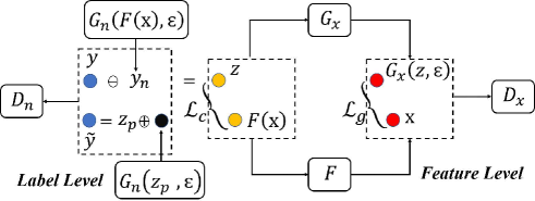
Figure 1: The proposed MGPLL model comprises five component networks: the conditional noise label generator, $G_{n}$, which models noise labels conditioning on the truth label at the label level; the feature level conditional data generator, $G_{x}$, generates data samples conditioning on the denoised label vectors; the discriminator, $D_{n}$, tries to maximally separate the generated candidate label vectors from the observed real ones; the discriminator, $D_{x}$, tries to maximally separate the generated samples from the real data; the prediction network, $F$, predicts the denoised label vector for each training sample, and together with $G_{x}$ forms bi-directional maps between the label and feature spaces.

Given a partial label training set $S=\{(\mathbf{x}_{i},\mathbf{y}_{i})\}\operatorname{}\limits_{i=1}^{n}$, where $\mathbf{x}_{i}\in\mathbb{R}^{d}$ is a d-dimensional feature vector for the $i$-th instance, and $\mathbf{y}_{i}\in\{0,1\}^{L}$ denotes the candidate label indicator vector associated with $\mathbf{x}_{i}$, which has multiple 1 values corresponding to the ground-truth label and the noise labels, the task is to learn a good multi-class prediction model. In real world scenarios, the irrelevant noise labels are typically not presented in a random manner, but rather correlated with the ground-truth label. In this section, we present a novel multi-level generative model for partial label learning, MGPLL. The model is illustrated in Figure 1. It models non-random noise labels using an adversarial conditional noise label generator $G_{n}$ with a corresponding discriminator $D_{n}$, and builds connections between the denoised label vectors and instance features using a label-conditioned feature level generator $G_{x}$ and a label prediction network $F$. The overall model learning problem corresponds to a minimax adversarial game, which conducts multi-level generator learning by matching the observed data in both the feature and label spaces, while boosting the correspondence relationships between features and labels to induce an accurate multi-class prediction model. Below we present the details of the two level generations, the prediction network, and the overall learning problem.

3.1 Conditional Noise Label Generation

The key challenge of partial label learning lies in the fact that ground-truth label is hidden among noise labels in the given candidate label set. As aforementioned, in real world partial label learning problems, the appearances of noise labels are typically not random, but rather correlated with the ground-truth labels. Hence we propose a conditional noise label generation model to model the appearances of the target-label dependent noise labels and match the observed candidate label distribution in the training data through adversarial learning.

Specifically, given a noise value sampled from a uniform distribution $\epsilon\sim P_{\epsilon}$ and a one-hot label indicator vector $\mathbf{z}$ sampled from a multinomial distribution $P_{\mathbf{z}}$, we use a noise label generator $G_{n}(\mathbf{z},\epsilon)$ to generate a noise label vector conditioning on the true label $\mathbf{z}$, which can be combined with ${\bf z}$ to form a generated candidate label vector $\mathbf{\tilde{y}}$, such that $\mathbf{\tilde{y}}=G_{n}(\mathbf{z},\epsilon)\oplus{\bf z}=\min(G_{n}(\mathbf{z},\epsilon)+{\bf z},1)$. We then adopt the adversarial learning principle to learn such a noise label generation model by introducing a discriminator $D_{n}({\bf y})$, which is a two-class classifier and predicts how likely a given label vector ${\bf y}$ comes from the real data instead of generated data. By adopting the adversarial loss of the Wasserstein Generative Adversarial Network (WGAN) pmlr-v70-arjovsky17a , our adversarial learning problem can be formulated as the following minimax optimization problem:

$$\min_{G_{n}}\max_{D_{n}} \quad\mathcal{L}^{n}_{adv}(G_{n},D_{n})=$$ (1)

$$\mathbb{E}_{(\mathbf{x}_{i},\mathbf{y}_{i})\sim S}D_{n}(\mathbf{y}_{i})-\mathbb{E}_{\mathbf{z}\sim P_{\mathbf{z}}\atop\epsilon\sim P_{\epsilon}}D_{n}(G_{n}(\mathbf{z},\epsilon)\oplus{\bf z})$$

Here the discriminator $D_{n}$ attempts to maximally distinguish the generated candidate label vectors from the observed candidate label indicator vectors in the real training data, while the generator $G_{n}$ tries to generate noise label vectors and hence candidate label vectors that are similar to the real data in order to maximally confuse the discriminator $D_{n}$. By playing a minimax game between the generator $G_{n}$ and the discriminator $D_{n}$, the adversarial learning is expected to induce a generator $G_{n}^{*}$ such that the generated candidate label distribution can match the observed candidate label distribution in the training data GAN . We adopted the training loss of WGAN here, as WGAN can overcome the mode collapse problem and have improved learning stability comparing to the standard GAN pmlr-v70-arjovsky17a .

Note although the proposed generator $G_{n}$ is designed to model true-label dependent noise labels, it can be easily modified to model random noise label distributions by simply dropping the label vector input to have $G_{n}(\epsilon)$.

3.2 Prediction Network

The ultimate goal of partial label learning is to learn an accurate prediction network $F$. To train a good predictor, we need to obtain denoised labels on the training data. For a candidate label indicator vector $\bf{y}$, if the noise label indicator vector ${\bf y}_{n}$ is given, one can simply perform label denoising as follows to obtain the corresponding true label vector ${\bf z}$:

$${\bf z}={\bf y}\ominus{\bf y}_{n}=\max({\bf y-y_{n}},0)$$ (2)

Here the operator “$\ominus$” is introduced to generalize the standard minus “$-$” operator into the non-ideal case, where the noise label indicator vector ${\bf y}_{n}$ is not properly contained in the candidate label indicator vector.

The generator $G_{n}$ presented in the previous section provides a mechanism to generate noise labels and denoise candidate label sets, but requires true target label vector as input. We can use the outputs of the prediction network $F$ to approximate the target true label vectors of the training data for candidate label denoising purpose with $G_{n}$, while using the denoised labels as the prediction target for $F$. Specifically, with the noise label generator $G_{n}$ and predictor $F$, we can perform partial label learning by minimizing the following classification loss on the training data $S$:

$$\operatorname*{min}\limits_{F,G_{{n}}}\quad \mathcal{L}_{c}(F,G_{{n}})=$$ (3)

$$\mathbb{E}_{\epsilon\sim P_{\epsilon}\quad\atop(\mathbf{x}_{i},\mathbf{y}_{i})\sim S}\;\ell_{c}\big{(}F(\mathbf{x}_{i}),\;\mathbf{y}_{i}\ominus G_{n}(F(\mathbf{x}_{i}),\epsilon)\big{)}$$

Although in the ideal case, the output vectors of $G_{n}$ and $F$ would be indicator label vectors, it is error-prone and difficult for neural networks to output discrete values. To pursue more reliable predictions and avoid overconfident outputs, $G_{{n}}$ and $F$ predict the probability of each class label being a noise label and ground-truth label respectively. Hence the loss function $\ell_{c}(\cdot,\cdot)$ in Eq.(3) above denotes a mean square error loss between the predicted probability of each label being the true label (through $F$) and its confidence of being a ground-truth label (through $G_{n}$).

3.3 Conditional Feature Level Data Generation

With the noise label generation model and the prediction network above, the observed training data in both the label and feature spaces are exploited to recognize the true labels and induce good prediction models. Next, we incorporate a conditional data generator $G_{x}({\bf z},\epsilon)$ at the feature level to map (denoised) label vectors in the label space into instances in the feature space, aiming to further strengthen the mapping relations between data samples and the corresponding labels, enhance label denoising and hence improve partial label learning performance. Specifically, given a noise value $\epsilon$ sampled from a uniform distribution $P_{\epsilon}$ and a one-hot label vector $\mathbf{z}$ sampled from a multinomial distribution $P_{\mathbf{z}}$, $G_{{x}}(\mathbf{z},\epsilon)$ generates an instance in the feature space that is corresponding to label ${\bf z}$. Hence given the training label vectors in $S$ denoised with $G_{n}$, the data generator $G_{x}$ is expected to regenerate the corresponding training instances in the feature space. This assumption can be captured using the following generation loss:

$$\mathcal{L}_{g}(F,G_{{n}},G_{{x}})=\mathbb{E}_{(\mathbf{x}_{i},\mathbf{y}_{i})\sim S\atop\epsilon_{1},\epsilon_{2}\sim P_{\epsilon}}\;\ell_{g}\big{(}G_{{x}}({\bf z}_{i},\epsilon_{2}),\mathbf{x}_{i}\big{)}$$ (4)

where ${\bf z}_{i}={\bf y}_{i}\ominus G_{n}(F({\bf x}_{i}),\epsilon_{1})$ denotes the denoised label vector for the $i$-th training instance, and $\ell_{g}(\cdot,\cdot)$ is a mean square error loss function.

Moreover, by introducing a discriminator $D_{x}({\bf x})$, which predicts how likely a given instance ${\bf x}$ is real, we can deploy an adversarial learning scheme to learn the generator $G_{x}$ through the following minimax optimization problem with the WGAN loss:

$$\operatorname*{min}\limits_{G_{{x}}}\operatorname*{max}\limits_{D_{{x}}}\;\; \mathcal{L}^{x}_{adv}(G_{{x}},D_{{x}})=$$ (5)

$$\mathbb{E}_{(\mathbf{x}_{i},\mathbf{y}_{i})\sim S}D_{{x}}(\mathbf{x}_{i})-\mathbb{E}_{\mathbf{z}\sim P_{\mathbf{z}}\atop\epsilon\sim P_{\epsilon}}D_{{x}}(G_{{x}}(\mathbf{z},\epsilon))$$

By playing a minimax game between $G_{x}$ and $D_{x}$, this adversarial learning is expected to induce a generator $G^{*}_{x}$ that can generate samples with the same distribution as the observed training instances. Hence the mapping relation from label vectors to samples induced by $G^{*}_{x}$ can also hold on the real training data, and should be consistent with the inverse mapping from samples to label vectors through the prediction network. Therefore, we can further consider an auxiliary classification loss on the generated data:

$$\mathcal{L}_{c^{\prime}}(F,G_{{x}})=\mathbb{E}_{\mathbf{z}\sim P_{\mathbf{z}}\atop\epsilon\sim P_{\epsilon}}\;\,\ell_{c^{\prime}}\big{(}F(G_{{x}}(\mathbf{z},\epsilon)),\mathbf{z}\big{)}$$ (6)

where $\ell_{c^{\prime}}(\cdot,\cdot)$ can be a cross-entropy loss between the label prediction probability vector and the sampled true label indicator vector.

3.4 Learning the MGPLL Model

By integrating the classification loss in Eq.(3), the adversarial losses in Eq.(1) and Eq.(5), the generation loss in Eq.(4) and the auxiliary classification loss in Eq.(6) together, MGPLL learning can be formulated as the following min-max optimization problem:

$$\operatorname*{min}\limits_{G_{{n}},G_{{x}},F}\ \operatorname*{max}\limits_{D_{{n}},D_{{x}}}\mathcal{L}_{c}(F,G_{{n}})+\mathcal{L}^{n}_{adv}(G_{{n}},D_{{n}})+$$

$$\quad\;\alpha\mathcal{L}^{x}_{adv}(G_{{x}},D_{{x}})+\beta\mathcal{L}_{g}(F,G_{{n}},G_{{x}})+\gamma\mathcal{L}_{c^{\prime}}(F,G_{{x}})$$ (7)

where $\alpha$, $\beta$ and $\gamma$ are trade-off hyperparameters. The learning of the overall model corresponds to a minimax adversarial game. We develop a batch-based stochastic gradient descent algorithm to solve it by conducting minimization over {$G_{n},G_{x},F$} and maximization over {$D_{n},D_{x}$} alternatively. The overall training algorithm is outlined in Algorithm 1.

Algorithm 1 Minibatch stochastic gradient descent.

Input: $S:$ the PL training set; $\alpha,\beta,\gamma$: the trade-off hyperparameters; $c$: the clipping parameter; $m$: minibatch size.

  for number of training iterations do

      Sample a minibatch $B$ of $m$ samples from $S$.

      Sample a $m$ noise values $\{\epsilon_{i}\}$ from a prior $P(\epsilon)$.

      Sample $m$ label vectors $\{\mathbf{z}_{i}\}$ from a prior $P_{\mathbf{z}}$.

      Update $D_{{n}},D_{{x}}$ by ascending their stochastic gradients:

       

$$\nabla_{\Theta_{\tiny D_{{n}},D_{{x}}}}\frac{1}{m}\operatorname*{\sum}\limits_{i=1}^{m}\left\{\!\!\!\!\begin{array}[]{l}\Big{(}D_{{n}}(\mathbf{y}_{i})-D_{{n}}(G_{{n}}(\mathbf{z}_{i},\epsilon_{i})\oplus{\bf z}_{i})\Big{)}\\ +\alpha\Big{(}D_{{x}}(\mathbf{x}_{i})-D_{{x}}(G_{{x}}(\mathbf{z}_{i},\epsilon_{i}))\Big{)}\end{array}\!\!\!\!\!\!\right\}$$

      $\Theta_{D_{\mathbf{n}},D_{\mathbf{x}}}\leftarrow\mathrm{clip}(\Theta_{D_{\mathbf{n}},D_{\mathbf{x}}},-c,c)$ (WGAN adjustment)

      Sample $m$ noise values $\{\overline{\epsilon}_{i}\}$ from a prior $P(\epsilon)$.

      Update $G_{\mathbf{n}},G_{\mathbf{x}},F$ by stochastic gradient descent:

       

$$\nabla_{\Theta_{\tiny G_{{n}},G_{{x}},F}}\frac{1}{m}\!\operatorname*{\sum}\limits_{i=1}^{m}\!\!\left\{\!\!\!\!\begin{array}[]{l}\ell_{c}(F(\mathbf{x}_{i}),\mathbf{y}_{i}\ominus G_{{n}}(F(\mathbf{x}_{i}),\epsilon_{i}))\\ -D_{{n}}(G_{{n}}(\mathbf{z}_{i},\epsilon_{i})\oplus{\bf z}_{i})\\ -\alpha D_{{x}}(G_{{x}}(\mathbf{z}_{i},\overline{\epsilon}_{i}))+\\ \beta\ell_{g}\big{(}G_{{x}}\big{(}\mathbf{y}_{i}\ominus G_{{n}}(F(\mathbf{x}_{i}),\epsilon_{i}),\overline{\epsilon}_{i}\big{)},\mathbf{x}_{i}\big{)}\\ +\gamma\ell_{c^{\prime}}F(G_{{x}}(\mathbf{z}_{i},\overline{\epsilon}_{i}),\mathbf{z}_{i})\end{array}\!\!\!\!\right\}$$

  end for

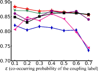
(a) ecoli

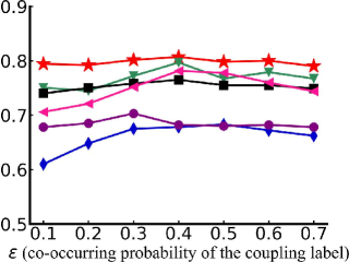
(b) vehicle

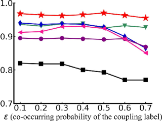
(c) segment

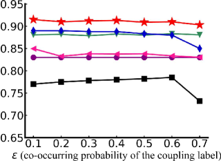
(d) satimage

Figure 2: Test accuracy of each comparison method changes as $\epsilon$ (co-occurring probability of the coupling label) increases from 0.1 to 0.7 (with 100% partially labeled examples $[p=1]$ and one false positive candidate label $[r=1]$).

4 Experiment

4.1 Datasets

We conducted experiments on both controlled synthetic PL datasets and a number of real-world PL datasets.

The synthetic datasets are generated from four UCI datasets, ecoli, vehicle, segment and satimage, which have 8, 4, 7 and 7 classes, and 336, 846, 2310 and 6,345 examples, respectively. From each UCI dataset, we generated synthetic PL datasets using three controlling parameters $p,r$ and $\epsilon$, following the controlling protocol in previous works wu2018towards ; Xu2019Enhancement ; Feng2019Retraining . Among the three parameters, $p$ controls the proportion of instances that have noise candidate labels, $r$ controls the number of false positive labels, and $\epsilon$ controls the probability of a specific false positive label co-occurring with the true label. Under different parameter configurations, multiple PL variants can be generated from each UCI dataset. In particular, we considered two settings. In the first setting, we consider random noise labels with the following three groups of configurations: (I) $r=1$, $p\in\{0.1,0.2,\cdot\cdot\cdot,0.7\}$; (II) $r=2$, $p\in\{0.1,0.2,\cdot\cdot\cdot,0.7\}$; (III) $r=3$, $p\in\{0.1,0.2,\cdot\cdot\cdot,0.7\}$. In the second setting, we consider the target label-dependent noise labels with the following configuration: (IV) $p=1$, $r=1$, $\epsilon\in\{0.1,0.2,\cdot\cdot\cdot,0.7\}$. In total, this provides us 112 (28 configurations $\times$ 4 UCI datasets) synthetic PL datasets.

Table 1: Characteristics of the real-world PL datasets.

Dataset	#Example	#Feature	#Class	avg.#CLs
FG-NET	1,002	262	78	7.48
Lost	1,122	108	16	2.23
MSRCv2	1,758	48	23	3.16
BirdSong	4,998	38	13	2.18
Yahoo! News	22,991	163	219	1.91

We used five real-world PL datasets that are collected from several application domains, including FG-NET panis2014overview for facial age estimation, Lost cour2011learning , Yahoo! News guillaumin2010multiple for automatic face naming in images or videos, MSRCv2 dietterich1994solving for object classification, and BirdSong briggs2012rank for bird song classification. The characteristics of the real-world PL datasets are summarized in Table 1.

4.2 Comparison Methods

We compared the proposed MGPLL approach with the following PL methods, each configured with the suggested parameters according to the respective literature:

• PL-KNN hullermeier2006learning : A k-NN based method which makes prediction with weighted voting.

• PL-SVM nguyen2008classification : A maximum-margin based method which maximizes the classification margin between candidate and non-candidate class labels.

• CLPL cour2011learning : A convex optimization based method for partial label learning.

• PALOC wu2018towards : An ensemble method which trains multiple binary classifies with the one-vs-one decomposition strategy and makes prediction by consulting all binary classifies.

• SURE Feng2019Retraining : A self-training based method which learns a confidence matrix of candidate labels with a maximum infinity norm regularization and trains the prediction model over the learned label confidence matrix.

4.3 Implementation Details

The proposed MGPLL model has five component networks, all of which are designed as multilayer perceptrons with Leaky ReLu activation for the middle layers. The noise label generator is a four-layer network with sigmoid activation in the output layer. The conditional data generator is a five-layer network with tanh activation in the output layer, while batch normalization is deployed in its middle three layers. The predictor is a three-layer network with softmax activation in the output layer. Both the noise label discriminator and the data discriminator are three-layer networks without activation in the output layer. The RMSProp tieleman2012lecture optimizer is used in our implementation and the mini-batch size m is set to 32. We selected the hyperparameters $\alpha$, $\beta$ and $\gamma$ from {0.001, 0.01, 0.1, 1, 10} based on the classification loss value $\mathcal{L}_{c}$ in the training objective function; that is, we chose their values that lead to the smallest training $\mathcal{L}_{c}$ loss.

Table 2: Win/tie/loss counts of pairwise t-test (at 0.05 significance level) between MGPLL and each comparison approach.

	MGPLL vs –
	SURE	PALOC	CLPL	PL-SVM
varying $p$ $[r=1]$	18/7/3	22/6/0	24/4/0	24/4/0
varying $p$ $[r=2]$	16/9/3	19/9/0	21/7/0	22/6/0
varying $p$ $[r=3]$	14/12/2	18/10/0	20/8/0	23/5/0
varying $\epsilon$ $[p,r=1]$	15/13/0	18/10/0	18/10/0	21/7/0
Total	63/41/8	77/35/0	83/29/0	90/22/0

4.4 Results on Synthetic PL Datasets

We conducted experiment on two types of synthetic PL datasets generated from the UCI datasets, with random noise labels and target label-dependent noise labels, respectively. For each PL dataset, ten-fold cross-validation is performed and the average test accuracy results are recorded. First we study the comparison results over the PL datasets with target label-dependent noise labels under the PL configuration setting IV. In this setting, a specific label is selected as the coupled label that co-occurs with the ground-truth label with probability $\epsilon$, and any other label can be randomly chosen as a noisy label with probability $1-\epsilon$. Figure 2 presents the comparison results for the configuration setting IV, where $\epsilon$ increases from 0.1 to 0.7 with $p=1$ and $r=1$. From Figure 2 we can see that the proposed MGPLL produces promising results. It consistently outperforms the other methods across different $\epsilon$ values on three datasets, while achieving remarkable gains on segment and satimage. We also conducted experiments on the PL datasets with random noise labels produced under PL configuration settings I, II and III, while MGPLL (with noise label generator $G_{n}(\epsilon)$) achieves similar positive comparison results as above. Due to the limitation of space, instead of including the comparison figures, we summarize the comparison results below with statistical significance tests.

To statistically study the significance of the performance gains achieved by MGPLL over the other comparison methods, we conducted pairwise t-test at 0.05 significance level based on the comparison results of ten-fold cross-validation over all the 112 synthetic PL datasets obtained for all different configuration settings. The detailed win/tie/loss counts between MGPLL and each comparison method are reported in Table 2, from which we have the following observations: (1) MGPLL achieves superior or at least comparable performance over PALOC, CLPL, and PL-SVM in all cases, which is not easy given the comparison methods have different strengths across different datasets. (2) MGPLL significantly outperforms PALOC, CLPL, and PL-SVM in 68.7%, 74.1%, and 80.3% of the cases respectively, and produces ties in the remaining cases. (3) MGPLL significantly outperforms SURE in 56.2% of the cases while achieves comparable performance in 36.6%, and is outperformed by SURE in only remaining 7.1% of the cases. (4) On the PL datasets with target label-dependent noise labels, we can see that MGPLL significantly outperforms SURE, PALOC, CLPL, and PL-SVM in 53.5%, 64.2%, 64.2%, and 75.0%, of the cases respectively. (5) It is worth noting that MGPLL is never significantly outperformed by any comparison methods on datasets with label-dependent noise labels. In summary, these results on the controlled PL datasets clearly demonstrate the effectiveness of MGPLL for partial label learning under different settings.

Table 3: Test accuracy (mean$\pm$std) of each comparison method on the real-world PL datasets. $\bullet/$$\circ$ indicates whether MGPLL is statistically superior$/$inferior to the comparison algorithm on each dataset (pairwise t-test at 0.05 significance level).

	MGPLL	SURE	PALOC	CLPL	PL-SVM	PL-KNN
FG-NET	0.079$\pm$0.024	0.068$\pm$0.032	0.064$\pm$0.019	0.063$\pm$0.027	0.063$\pm$0.029	0.038$\pm$0.025$\bullet$
FG-NET(MAE3)	0.468$\pm$0.027	0.458$\pm$0.024	0.435$\pm$0.018$\bullet$	0.458$\pm$0.022	0.356$\pm$0.022$\bullet$	0.269$\pm$0.045$\bullet$
FG-NET(MAE5)	0.626$\pm$0.022	0.615$\pm$0.019	0.609$\pm$0.043$\bullet$	0.596$\pm$0.017$\bullet$	0.479$\pm$0.016$\bullet$	0.438$\pm$0.053$\bullet$
Lost	0.798$\pm$0.033	0.780$\pm$0.036$\bullet$	0.629$\pm$0.056	0.742$\pm$0.038$\bullet$	0.729$\pm$0.042$\bullet$	0.424$\pm$0.036$\bullet$
MSRCv2	0.533$\pm$0.021	0.481$\pm$0.036$\bullet$	0.479$\pm$0.042$\bullet$	0.413$\pm$0.041$\bullet$	0.461$\pm$0.046$\bullet$	0.448$\pm$0.037$\bullet$
BirdSong	0.748$\pm$0.020	0.728$\pm$0.024$\bullet$	0.711$\pm$0.016$\bullet$	0.632$\pm$0.019$\bullet$	0.660$\pm$0.037$\bullet$	0.614$\pm$0.021$\bullet$
Yahoo! News	0.678$\pm$0.008	0.644$\pm$0.015$\bullet$	0.625$\pm$0.005$\bullet$	0.462$\pm$0.009$\bullet$	0.629$\pm$0.010$\bullet$	0.457$\pm$0.004$\bullet$

Table 4: Comparison results of MGPLL and its five ablation variants.

	MGPLL	CLS-w/o-advn	CLS-w/o-advx	CLS-w/o-g	CLS-w/o-aux	CLS
FG-NET	0.079$\pm$0.024	0.061$\pm$0.024	0.072$\pm$0.020	0.068$\pm$0.029	0.076$\pm$0.022	0.057$\pm$0.016
FG-NET(MAE3)	0.468$\pm$0.027	0.430$\pm$0.029	0.451$\pm$0.032	0.436$\pm$0.038	0.456$\pm$0.033	0.420$\pm$0.420
FG-NET(MAE5)	0.626$\pm$0.022	0.583$\pm$0.055	0.605$\pm$0.031	0.590$\pm$0.045	0.612$\pm$0.044	0.570$\pm$0.034
Lost	0.798$\pm$0.033	0.623$\pm$0.037	0.754$\pm$0.032	0.687$\pm$0.026	0.782$\pm$0.043	0.609$\pm$0.040
MSRCv2	0.533$\pm$0.021	0.472$\pm$0.030	0.480$\pm$0.038	0.497$\pm$0.031	0.526$\pm$0.036	0.450$\pm$0.037
BirdSong	0.748$\pm$0.020	0.728$\pm$0.010	0.732$\pm$0.011	0.716$\pm$0.011	0.742$\pm$0.024	0.674$\pm$0.016
Yahoo! News	0.678$\pm$0.008	0.645$\pm$0.008	0.675$\pm$0.009	0.648$\pm$0.014	0.671$\pm$0.012	0.610$\pm$0.015

4.5 Results on Real-World PL Datasets

We compared the proposed MGPLL method with the comparison methods on five real-world PL datasets. For each dataset, ten-fold cross-validation is conducted, while the mean test accuracy as well as the standard deviation results are reported in Table 3. Moreover, statistical pairwise t-test at 0.05 significance level is conducted to compare MGPLL with each comparison method based on the results of ten-fold cross-validation. The significance results are indicated in Table 3 as well. Note that the average number of candidate labels (avg.#CLs) of FG-NET dataset is quite large, which causes poor performance for all the comparison methods. For better evaluation of this facial age estimation task, we employ the conventional mean absolute error (MAE) zhang2016partial to conduct two extra experiments. Two extra test accuracies are reported on the FG-NET dataset where a test sample is considered to be correctly predicted if the difference between the predicted age and the ground-truth age is less than 3 years (MAE3) or 5 years (MAE5). From Table 3 we have the following observations: (1) Comparing with all the five PL methods, MGPLL consistently produces the best results on all the datasets, with remarkable performance gains in many cases. For example, MGPLL outperforms the best alternative comparison methods by 5.2%, 3.4% and 2.0% on MSRCv2, Yahoo! News and Birdsong respectively. (2) Out of the total 35 comparison cases (5 comparison methods $\times$ 7 datasets), MGPLL significantly outperforms all the comparison methods across 77.1% of the cases, and achieves competitive performance in the remaining 22.9% of cases. (3) It is worth noting that the performance of MGPLL is never significantly inferior to any other comparison methods. These results on the real-world PL datasets again validate the efficacy of the proposed method.

4.6 Ablation Study

The objective function of MGPLL contains five loss terms: classification loss, adversarial loss at the label level, adversarial loss at the feature level, generation loss and auxiliary classification loss. To assess the contribution of each part, we conducted an ablation study by comparing MGPLL with the following ablation variants: (1) CLS-w/o-advn, which drops the adversarial loss at the label level. (2) CLS-w/o-advx, which drops the adversarial loss at the feature level. (3) CLS-w/o-g, which drops the generation loss. (4) CLS-w/o-aux, which drops the auxiliary classification loss. (5) CLS, which only uses the classification loss by dropping all the other loss terms. The comparison results are reported in Table 4. We can see that comparing to the full model, all five variants produce inferior results in general and have performance degradations to different degrees. This demonstrates that the different components in MGPLL all contribute to the proposed model to some extend. From Table 4, we can also see that the variant CLS-w/o-advn has a relatively larger performance degradation by dropping the adversarial loss at the label level, while the variant CLS-w/o-aux has a small performance degradation by dropping the auxiliary classification loss. This makes sense as by dropping the adversarial loss for learning noise label generator, the generator can produce poor predictions and seriously impact the label denoising of the MGPLL model. This suggests that our non-random noise label generation through adversarial learning is a very effective and important component for MGPLL. For CLS-w/o-aux, as we have already got the classification loss on real data, it is reasonable to see that the auxiliary classification loss on generated data can help but is not critical. Overall, the ablation study results suggest that the proposed MGPLL is effective.

5 Conclusion

In this paper, we proposed a novel multi-level generative model, MGPLL, for partial label learning. MGPLL uses a conditional label level generator to model target label dependent non-random noise label appearances, which directly performs candidate label denoising, while using a conditional feature level generator to generate data samples from denoised label vectors. Moreover, a prediction network is incorporated to predict the denoised true label of each instance from its input features, which forms inverse mappings between labels and features, together with the data feature generator. The adversarial learning of the overall model simultaneously identifies true labels of the training instances from both the observed data features and the observed candidate labels, while inducing accurate prediction networks that map input feature vectors to (denoised) true label vectors. We conducted extensive experiments on real-world and synthesized PL datasets. The proposed MGPLL model demonstrates the state-of-the-art PL performance.

References

- [1] M. Arjovsky, S. Chintala, and L. Bottou. Wasserstein generative adversarial networks. In Proceedings of the International Conference on Machine Learning (ICML), 2017.
- [2] F. Briggs, X. Z. Fern, and R. Raich. Rank-loss support instance machines for miml instance annotation. In Proceedings of the ACM SIGKDD international conference on Knowledge discovery and data mining (KDD), 2012.
- [3] T. Cour, B. Sapp, and B. Taskar. Learning from partial labels. Journal of Machine Learning Research, 12(May):1501–1536, 2011.
- [4] T. G. Dietterich and G. Bakiri. Solving multiclass learning problems via error-correcting output codes. Journal of artificial intelligence research, 2:263–286, 1994.
- [5] L. Feng and B. An. Leveraging latent label distributions for partial label learning. In International Joint Conference on Artificial Intelligence (IJCAI), 2018.
- [6] L. Feng and B. An. Partial label learning by semantic difference maximization. In International Joint Conference on Artificial Intelligence (IJCAI), 2019.
- [7] C. Gong, T. Liu, Y. Tang, J. Yang, J. Yang, and D. Tao. A regularization approach for instance-based superset label learning. IEEE transactions on cybernetics, 48(3):967–978, 2018.
- [8] I. Goodfellow, J. Pouget-Abadie, M. Mirza, B. Xu, D. Warde-Farley, S. Ozair, A. Courville, and Y. Bengio. Generative adversarial nets. In Advances in Neural Information Processing Systems (NeurIPS), 2014.
- [9] M. Guillaumin, J. Verbeek, and C. Schmid. Multiple instance metric learning from automatically labeled bags of faces. In European Conference on Computer Vision (ECCV), 2010.
- [10] E. Hüllermeier and J. Beringer. Learning from ambiguously labeled examples. Intelligent Data Analysis, 10(5):419–439, 2006.
- [11] R. Jin and Z. Ghahramani. Learning with multiple labels. In Advances in neural information processing systems (NeurIPS), 2003.
- [12] F. Lei and B. An. Partial label learning with self-guided retraining. In AAAI Conference on Artificial Intelligence (AAAI), 2019.
- [13] J. Luo and F. Orabona. Learning from candidate labeling sets. In Advances in Neural Information Processing Systems (NeurIPS), 2010.
- [14] N. Nguyen and R. Caruana. Classification with partial labels. In Proceedings of the ACM SIGKDD international conference on Knowledge discovery and data mining (KDD), 2008.
- [15] G. Panis and A. Lanitis. An overview of research activities in facial age estimation using the fg-net aging database. In European Conference on Computer Vision (ECCV), 2014.
- [16] C.-Z. Tang and M.-L. Zhang. Confidence-rated discriminative partial label learning. In AAAI Conference on Artificial Intelligence (AAAI), 2017.
- [17] T. Tieleman and G. Hinton. Lecture 6.5-rmsprop: Divide the gradient by a running average of its recent magnitude. COURSERA: Neural networks for machine learning, 4(2):26–31, 2012.
- [18] D.-B. Wang, L. Li, and M.-L. Zhang. Adaptive graph guided disambiguation for partial label learning. In Proceedings of the 25th ACM SIGKDD International Conference on Knowledge Discovery & Data Mining, pages 83–91, 2019.
- [19] X. Wu and M.-L. Zhang. Towards enabling binary decomposition for partial label learning. In International Joint Conference on Artificial Intelligence (IJCAI), 2018.
- [20] N. Xu, J. Lv, and X. Geng. Partial label learning via label enhancement. In AAAI Conference on Artificial Intelligence (AAAI), 2019.
- [21] Z. Zeng, S. Xiao, K. Jia, T.-H. Chan, S. Gao, D. Xu, and Y. Ma. Learning by associating ambiguously labeled images. In Proceedings of the IEEE Conference on Computer Vision and Pattern Recognition (CVPR), 2013.
- [22] M.-L. Zhang and F. Yu. Solving the partial label learning problem: An instance-based approach. In International Joint Conference on Artificial Intelligence (IJCAI), 2015.
- [23] M.-L. Zhang, B.-B. Zhou, and X.-Y. Liu. Partial label learning via feature-aware disambiguation. In Proceedings of the ACM SIGKDD International Conference on Knowledge Discovery and Data Mining (KDD), 2016.