The VVV Infrared Variability Catalog (VIVA-I)

Resumo

High extinction and crowding create a natural limitation for optical surveys towards the central regions of the Milky Way where the gas and dust are mainly confined. Large scale near-IR surveys of the Galactic Plane and Bulge are a good opportunity to explore open scientific questions as well as to test our capability to explore future datasets efficiently. Thanks to the VISTA Variables in the Vía Láctea (VVV) ESO Public Survey it is now possible to explore a large number of objects in those regions. This paper addresses the variability analysis of all VVV point sources having more than $10$ observations in VVVDR4 using a novel approach. In total, the near-IR light curves of $288,378,769$ sources were analysed using methods developed in the New Insight Into Time Series Analysis project. As a result, we present a complete sample having $44,998,752$ variable star candidates (VVV-CVSC), which include accurate individual coordinates, near-IR magnitudes ($ZYJH_{s}$), extinctions $A(K_{s})$, variability indices, periods, amplitudes, among other parameters to assess the science. Unfortunately, a side effect of having a highly complete sample, is also having a high level of contamination by non-variable (contamination ratio of non-variables to variables is slightly over 10:1). To deal with this, we also provide some flags and parameters that can be used by the community to decrease the number of variable candidates without heavily decreasing the completeness of the sample. In particular, we icross-dentified $339,601$ of our sources with Simbad and AAVSO databases, which provide us with information for these objects at other wavelegths. This subsample constitutes a unique resource to study the corresponding near-IR variability of known sources as well as to assess the IR variability related with X-ray and Gamma-Ray sources. On the other hand, the other $\sim 99.5\%$ sources in our sample constitutes a number of potentially new objects with variability information for the heavily crowded and reddened regions of the Galactic Plane and Bulge. The present results also provide an important queryable resource to perform variability analysis and to characterize ongoing and future surveys like TESS and LSST.

1 Introduction

The first infrared (IR) light curve was probably that obtained for the Cepheid Zeta Geminorum ($\zeta$ Gem) by John S. Hall using a caesium oxide photoelectric cell (Hall, 1932, 1934). The author found that the infrared maximum (at $7400\AA$) of the light curve occurs at $\sim 0.024$ periods later than that observed in optical light curves (Hoffleit, 1987). Indeed, the characterization of different physical processes is better enabled when photometry across the whole electromagnetic spectrum is available. On the other hand, the interstellar environment is noticeably more transparent in IR and Near-IR (NIR) light than at visible light. Thus, photometric surveys at infrared wavelengths can reveal different physical processes and explore unknown Milky Way (MW) regions at low Galactic latitudes that are usually obscured at visible wavelengths by the absorption of light by the interstellar medium. Atmospheric transparency is a strong function of wavelength, and many parts of the electromagnetic spectrum are not visible from the ground, and the technical capabilities of instruments tend to be poorer outside of the visible because the technologies are newer and have fewer commercial applications: hence the scientific discoveries have been limited by technology. The MW inner structure and details of its formation and evolution have been poorly understood due to the lack of variability datasets in these regions. Gas and dust in MW are mostly confined to the disk, where high extinction and crowding limit the usefulness of optical wavelengths. According to this natural limitation, most current optical surveys avoid the innermost MW plane. The detailed shapes of disk galaxies can hold clues to understanding the role that dynamical instabilities, hierarchical merging, and dissipative collapse played in the assembly history of the entire host galaxy (Athanassoula, 2005). In particular, the resolved stellar populations of the bulge, in connection with those of the disc and halo, provide us with a unique laboratory to investigate the fossil records of such fundamental processes (see Gonzalez & Gadotti, 2016).

There are many large new studies of stellar variability due to improved telescopes/instruments with large entente and in particular the better access to publicly available datasets from large variability surveys. For instance, at optical wavelengths this has led to improvements in the understanding of the stellar astrophysics of rotational modulation of stellar activity (e.g. McQuillan et al., 2014; Ferreira Lopes et al., 2015c; Cortés et al., 2015; Suárez Mascareño et al., 2016; Balona et al., 2019), stellar pulsation (e.g. Andersson & Kokkotas, 1996; García et al., 2014; Angeloni et al., 2014a; Ferreira Lopes et al., 2015b; Catelan & Smith, 2015; Braga et al., 2019), exoplanets (e.g. Fernández et al., 2006; Minniti et al., 2007; Pietrukowicz et al., 2010; Paz-Chinchón et al., 2015; Gillon et al., 2017; Almeida et al., 2019; Cortés et al., 2019), young stellar objects (e.g. Contreras Peña et al., 2017; Contreras Pena et al., 2017; Lucas et al., 2017; Guo et al., 2019), novae (e.g. Saito et al., 2012; Banerjee et al., 2018), gravitational microlensing events (e.g. Minniti et al., 2015; Navarro et al., 2017, 2018, 2019), and eclipsing binaries (e.g. Torres et al., 2010; Angeloni et al., 2012; Hełminiak et al., 2013; Deleuil et al., 2018). On the other hand, new studies based on IR variability data at low Galactic latitudes may now become more accessible.

For the past 10 years the ESO Public Survey VVV Survey and its extension VVVX (VISTA Variables in the Via Lactea, VVV eXtended, respectively) have been mapping the NIR variability ($K_{s}$-band), of the Milky Way Bulge and the adjacent southern Disk, complemented by multi-colour observations. The VVV included the ZYJH$K_{s}$ bands (Minniti et al., 2010), whereas VVVX was restricted to the JHKs bands. The variability campaign in the $K_{s}$-waveband observed about $100$ $K_{s}$ epochs per field over the period 2010-2016 (for more details see Sect. 2).

The VVV complements other public optical and mid-IR variability surveys of the Milky Way such as the Optical Gravitational Lensing Experiment (OGLE - Soszyński et al., 2009), Gaia (Perryman, 2005), the Transiting Exoplanet Survey Satellite (TESS - Ricker et al., 2015), the Panoramic Survey Telescope and Rapid Response System (Pan-STARRS - Kaiser et al., 2002), A High-cadence All-sky Survey System (ATLAS - Tonry et al., 2018), Zwicky Transient Facility (ZTF - Bellm et al., 2019) as well as the next generation of surveys like PLAnetary Transits and Oscillation of stars (PLATO - Rauer et al., 2014), the Large Synoptic Survey Telescope (LSST - Ivezić et al., 2019) and the Wide-field Infrared Survey Explorer (Mainzer et al., 2011) by covering the dust-encompassed central bulge regions and far-side of the disk at higher spatial resolution than is possible at longer wavelengths and adding additional important spectral information to all objects observed.

Large volumes of data containing potential scientific results are still unexplored or delayed due to our current inventory of tools that are unable to select clean samples. Despite great efforts having been undertaken, we run the risk of underusing a large part of these data. In the last decade, much effort has been made in automating, for example, the classification of variable stars (e.g. Debosscher et al., 2007; Ivezic et al., 2008; Richards et al., 2011; Kim et al., 2011; Bloom et al., 2012; Pichara & Protopapas, 2013; Nun et al., 2014; Angeloni et al., 2014b; Pichara et al., 2016; Cabrera-Vives et al., 2017; Benavente et al., 2017; Graham et al., 2017; Valenzuela & Pichara, 2018). Usually these methods invest lots of efforts to extract features able to represent the peculiarities of different signals. These features can vary in number from a few to many tens of parameters (e.g. Kim et al., 2014; Nun et al., 2015). On the other hand, approaches where the light curves are transformed into a two-dimensional array to perform classification with a convolutional neural network (Mahabal et al., 2017) and unsupervised feature learning algorithms (Mackenzie et al., 2016) can find most of the underlying patterns that represent every light curve. Moreover, approaches using automatic learning of features are also being tested (e.g. Mackenzie et al., 2016). Indeed, the light curves of the same source observed by different surveys would normally have different values for their features. However, if we use noise and periodicities to match distributions of features we avoid having to re-train from scratch for each new classification problem (Long et al., 2012).

The classification procedure presupposes that all parameters are accurately measured. For instance, a few percent of observed stars have non-stochastic variability and $75\%$ of the parameters used to characterize light curves are derived from variability periods (Richards et al., 2011). Inaccurate parameters may lead to a considerable increase of machine processing time and greater misclassification rates (e.g. Dubath et al., 2011; Ferreira Lopes et al., 2015a). On the other hand, the New Insight into Time Series Analysis (NITSA) project took a step back in order to review and improve all time-varying procedures (Ferreira Lopes & Cross, 2016, 2017; Ferreira Lopes et al., 2018b). As a result, the NITSA project provides optimized constraints to select a clean sample, i.e. a sample having only variable stars, on which the classification methods can be applied properly.

Unlike many variability surveys, the VVV survey is carried out in the near-IR. Despite several fundamental advantages, mostly due to the ability to probe deeper into the heavily reddened regions, the use of near-IR also presents important challenges. In particular, high-quality templates that are needed for training the automated variable star classification algorithms are not available (e.g. Debosscher et al., 2007; Richards et al., 2011; Dubath et al., 2012; Bloom et al., 2012; Pichara et al., 2016). Many variable-star classes have not yet been observed extensively in the near-IR, so that proper light curves are entirely lacking for these classes. The VVV Templates Project (Angeloni et al., 2014b) has turned out to be a large observational effort in its own right, aimed at creating the first database on stellar variability in the near-IR, i.e. producing a large database of well-defined, high-quality, near-IR light curves. This project is in working progress and the variability analysis of the entire VVV database will be a very important step for such achievements. In order to reduce misclassification and mislabelling, accurate detections of true stellar variations are required. Moreover, the algorithms of classification need phased data to extract the main light curve features.

NITSA results were used to analyze the largest NIR survey of the MW bulge and disk. The text is organized as follows. Section 2 describes the VVV processing and in particular the multi-epoch pawprint data. The variability analysis is described in Sect. 3, where the discrimination of sources into correlated and non correlated data is presented (see Sects. 3.2 and 3.3). In particular, all constraints used to perform this step are tested on real data (see Sect. 3.4). Section 4.1 discusses the variable stars previously identified in the literature. These sources were used to check the reliability of the variability periods determined by us in Sect. 4.2. Next, we discuss using the height of the periodogram peaks (related to the likelihood that the frequency is periodic), for the different methods, to produce more reliable samples in order to reduce the misselection in Sect. 4.4. A new approach that improves the VVV data quality was proposed recently and hence we present the major implications in the current work 6. Discussions and final remarks are presented in Sects. 5 and 7. All parameters released in this work are described in Appendix A.

2 Data

The VVV is an ESO public survey that uses the Visible and Infrared Survey Telescope for Astronomy (VISTA) to map the bulge ($-10.0^{\circ}\lesssim l\lesssim+10.5^{\circ}$ and $-10.3^{\circ}\lesssim b\lesssim+5.1^{\circ}$) and the inner southern part of the Galactic disk ($294.7^{\circ}\lesssim l\lesssim+350.0^{\circ}$ and $-2.25^{\circ}\lesssim b\lesssim+2.25^{\circ}$) of our Galaxy using five near-IR wavebands (Z, Y, J, H and $K_{s}$) plus a variability campaign in $K_{s}$ waveband over the period 2010-2017 (Minniti et al., 2010).

We select our data from the VISTA Science Archive(VSA Cross et al., 2012), and in particular from the VVVDR4 release, which contains all VVV data up to the end of ESO period P91 (30/09/2013). The VISTA data comes as two types of image product with derived catalogues: pawprint and tile. We use the pawprint data throughout our analysis, since these measurements are observed in a way which allows us to use correlation indices. However, the standard products, and tables used for light-curves in the VVVDR4 release contain tile data, so some additional linking, as described below, is necessary to create light-curves from pawprint data.

The VIRCAM instrument on the VISTA telescope has 16 detectors, arranged in a $4\times 4$ pattern, with $90\%$ of a detector separation between each detector in the x-direction and $42.5\%$ in the y-direction. An individual observation labelled as a normal in the VSA is a multi-extension FITS file containing 16 image extensions, one for each detector. Several of these frames are jittered and co-averaged to form pawprint stacks. We use the catalogues from these in our analysis. 6 pawprint stacks are mosaiced together to form a 1.5 sq. deg. tile. These pawprints are arranged in a 2 by 3 grid, with a shift of almost one-detector in the x-direction and almost a half-detector in the y-direction, so that a typical part of the tile has twice the integration time. The VVV pointings are divided into different disk and bulge tile pointings which are labelled from d001 to d152 and from b201 to b396, respectively.

We have decided to use stacked pawprint photometry for the following reasons:

• Our analysis relies heavily on correlation indices and the overlapping pawprints within a tile provide between 2 to 6 independent measurements on short timescales (i.e. timescales much shorter than the epoch to epoch timescales, and therefore much shorter than the timescales of variability that we can measure), and can be considered to be correlated.

• Tile photometry extraction is a complex process and corrections for saturation, scattered light, aperture loss and distortion are more difficult to model in tiles. These problems arise because both the sky and point-spread-function (PSF) is highly variable in the near-infrared on time-scales shorter than observation length of the tile, so the individual pawprints have different values.

• VVVDR4, on which this version of VIVA is based, is on CASU version 1.3, and the newer version 1.5 includes many improvements to tile photometry, but the pawprint photometry remains the same apart from some zeropoint changes.

• While tiles have twice the exposure times of the pawprint stacks this does not always give the much increased depth in the crowded regions of the VVV bulge where source confusion is significant.

• There are typically twice as many pawprint measurements as tile measurements.

The raw data is processed by the Cambridge Astronomy Survey Unit (CASU Irwin et al., 2004) to produce the science quality stacked pawprint frames and standard $1.5$ sq. deg. tile frames and the catalogues from both image types. Up to date details about the nightly image and catalogue processing and calibration can be found at CASU. These images and catalogues are stored in FITS format and are transferred to the VSA, where further processing is done to create deeper images and catalogues, band-merged products, light-curves and simple variability statistics and crossmatches to multi-wavelength surveys, which are stored as tables in a SQLServer relational database management system (RBDMS). This allows scientists to rapidly select data, and only download what is relevant to their science case. In addition, these VDFS products are linked to other products developed by the VVV team, such as proper-motion catalogues Smith et al. (2018), or PSF photometry catalogues (e.g. Alonso-García et al., 2018). The VIVA catalog provided in the present paper will also be linked into the VSA, so it can be searched along with all the other VVV data and be used as part of complex queries that can select out particular samples of variable stars.

Light-curves can be extracted from the VSA VVVDR4 database using the vvvSourceXDetectionBestMatch table. However, this is based on tile detections, so to get the pawprint light-curves, we must join to the vvvTilePawprint table. An example SQL selection is shown in App B.

Light-curves in the VSA do not just link all frames in a tile pointing, but also find all matches in overlapping pointings (see Cross et al., 2009). If a star is in a region overlapping two tiles, where there have been 49 observations in the first and 53 in the second, and it is in a region of the first where it has measurements on 2 pawprints and of the second where it has measurements on 4 pawprints, we have 310 pawprint measurements of the star altogether.

The overlaps and short time between the pawprint measurements return data that match the necessary conditions to analyse variability using correlated indices (Ferreira Lopes & Cross, 2016, 2017), i.e. two or more measurements close in time, where the interval between the measurements used in a correlation are much less than the variability period. The correlated indices only provided trustful information about variability under this condition. The conditions for correlation are discussed in detail in Ferreira Lopes & Cross (2016), where the case of VISTA observations is also considered.

We have used the standard aperture-corrected aperture photometry in our analysis and in particular the default aperture of 1.0 arcsec radius (aper3, named as A3) for the photometry as it usually gives the best signal-to-noise for the typical seeing of VVV data (see Ferreira Lopes & Cross, 2017, for more details). This has a radius of 3 pixels and contains $\sim 75\%$ of the total flux in stellar images, and most of the seeing dependency is removed by the aperture-correction. However, we must keep in mind that, mainly in crowded regions, nearby stars can affect the observations by adding an additional noise component from deblending images that relies on some imperfect modelling (e.g. Cross et al., 2009; Contreras Ramos et al., 2017; Alonso-García et al., 2018; Medina et al., 2018). For such regions, the PSF photometry is being performed by VVV teams, e.g. (Alonso-Garcia, 2018; Surot et al., 2019).

3 Selection of Targets

The selection of variable stars using variability indices is mandatory because the later steps on variability analysis, like the detection of variability periods, are more time-consuming, so an early reduction in the number of possible targets leads to significantly less processing overall. The detection of reliable variations is intrinsically related to the number of observations since the statistical significance of the parameters used to discriminate variable stars from noise increases with the number of measurements. Fewer correlated measurements are required to compute correlated variability indices than the number of measurements needed to calculate non-correlated indices (statistical parameters) to the same accuracy. The number of observations required to compute reliable statistical parameters is not analytically defined. On the other hand, five is the minimum number of correlated measurements required to use correlated flux independent indices (for more details see Ferreira Lopes & Cross, 2016). Indeed, this limit can be extrapolated for all correlated indices. The efficiency rate of correlated indices is higher than non-correlated indices and hence correlated indices will be adopted in preference when they are available.

Photometric surveys can be divided into two main groups from the viewpoint of the number of observations: databases where the variability signal can be viewed in time, i.e. very well-sampled light-curves like CoRoT and Kepler light curves, and those ones which the variability signal can only be observed in the folded phase diagram like the large majority of sources observed by the VVV survey. For the latter ones, the variability indices will not be enough to determine the reliability of signals. Therefore, the variability periods are required to create phase diagrams for forthcoming analysis. To determine the period accurately we need enough measurements to cover all the main variability phases. For instance, some eclipsing binaries have eclipses that only cover a small fraction of the phase diagram and hence the signal can be lost if this region is not covered or only very sparsely covered, for example Algol type stars (see the OGLEII DIA BUL-SC35 V1058 in Fig. 6 and OGLEII DIA BUL-SC19 V4104 in Fig. 7). The lack of coverage of specific phases is less of a problem if the variability signature is a more smoothly varying signal along the whole phase diagram, like pulsating variable stars. Therefore, a reasonable number of measurements ($N$) is required to determine correctly the period and variability signature, but this is dependent on the type of variable star.

Photometric time series can be divided in four main groups in terms of variability indices and variability periods, as following:

• Noise (noise) - non-variable stars with random variations due to noise, which have variability indices that are consistent with the a non-variable source with noise or variations below the detection limit;

• Misclassified sources (MIS) - variable stars having variability indices around the noise level or noisy data having variability indices larger than that expected for the noise. As a result we will miss some real variable stars as well as including some noisy data in the target list;

• Variable stars with a non-detected variability period (VSNP) - variable stars where no variability period was detected either because they are aperiodic or the measurements were not sufficient to recover the period. This class also includes those sources having enough variation to be detected by variability indices but the data quality are not good enough to determine the light curve morphology, like saturated LPVs.

• Periodic variable stars (VSP) - variable stars where the variability period detected returns a smooth phase diagrams.

Indeed, statistical fluctuations, a small number of good measurements ($N$), outliers, correlated-noise, and seasonal variations are factors that are usually present in the data and hence a fraction of MIS are expected. The MIS rate varies for a particular dataset when using different techniques (Ferreira Lopes & Cross, 2016, 2017). On the other hand, the MIS rate also depends on the signal-to-noise distribution of the reliable signals as well as the data quality. The present work concerns the selection of VSNP and VSP targets observed by the VVV survey.

3.1 VVV Data Analysis

The New Insights into Time-Series Analysis (NITSA) project reviewed and improved the variability indices and the selection criteria for variable star candidates (Ferreira Lopes & Cross, 2016, 2017). The authors defined the criteria to determine which sources that can be analyzed with variability indices based on correlation measurements. Therefore, the data must be separated into two subsets: Correlated-Data (CD) and Non-Correlated Data (NCD), i.e those sources that should be analysed using correlated indices and non-correlated (statistical parameters) variability indices, respectively. The CD set includes those sources having more than 4 correlated measurements. The remaining data must be labelled as NCD. This identification is crucial to ensure the correct use of the variability indices. Non-correlated indices are not dependent on the arrangement of the observations and hence they can be computed for all sources. Therefore, both correlated and non-correlated variability indices can be combined to analyze CD sources while the NCD can only be analyzed using non-correlated variability indices. The correlated indices are more efficient than non-correlated indices (see left panel Fig. 8 of Ferreira Lopes & Cross, 2017), giving much better discrimination if available, so should be used if possible.

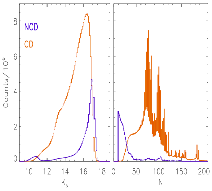
Figura 1: Histograms of $K_{s}$ magnitude and number of measurements ($N$) for the VVV initial sample. The results for both NCD (black lines) and CD (orange lines) are shown.

The observations of VVV pawprints necessary for the creation of tiles (see Sect 2) provide correlated data as a standard VISTA product, so we can optimize the search for variable stars since the correlated indices are freely available. Typically the observations necessary to make all 6 pawprint stacks in a tile are taken within $400s$, including the readout time that allows accurate correlated indices for variable stars having periods less than $\sim 130$min. The released table contains the values of non-correlated indices for NCD and CD data while the correlated indices only for the latter (for more details see Sects. 3.2 and 3.3).

All VVV sources having more than $10$ measurements were considered in the current work. An initial sample of $288,378,769$ VVV sources found in the DR4 release were analyzed in the present work. The interval time between consecutive measurements of $0.01$days was used to select close observations. These measurements were used to compute the correlated indices and determine the number of correlations (for more details see Ferreira Lopes & Cross, 2016). VVV data having more than four correlated measurements were labelled as CD otherwise NCD. About $82\%$ of the initial sample corresponds to CD type while the remaining sources are NCD. The NCD sources are mostly those which are in the single exposure "ears"of each tile, and a small number of faint sources which were not detected on many frames. Indeed, those measurements having quality bit flags corresponding to more serious conditions were removed. These were measurements with flags with values larger than 256.

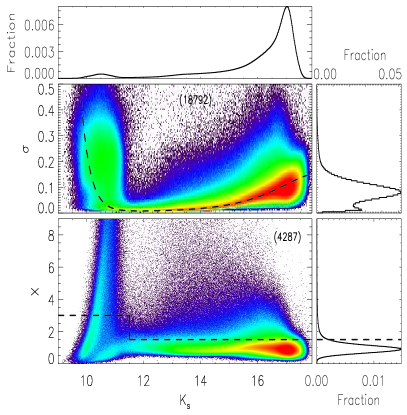
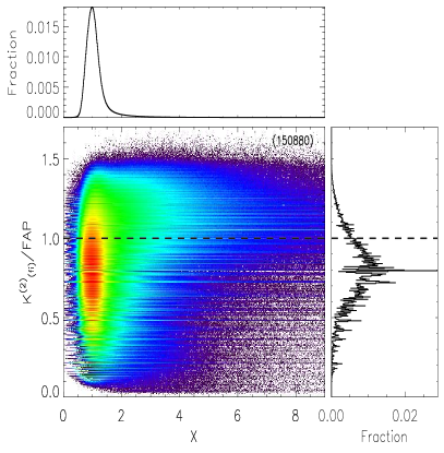
Figura 2: Relative density plots of $\sigma$ (upper left panel) and $X$ parameters (lower left panel) as function of magnitude as well as the $K_{(fi)}^{(2)}/Fap$ versus $X$ (right panel) index for our initial sample. The noise model is set by dark dashed line (upper left panels) while this line in the lower left panel and right panel mark the cut-off above which the variable star candidates of non-correlated and correlated data were selected, respectively. The histograms at the top and right side show the normalized distribution of x and y axis respectively.

Figure 1 shows the histograms of $K_{s}$ magnitude and number of measurements ($N$) for the VVV initial sample where the NCD and CD samples are set by colours. The faint and bright stars contribute about $84\%$ and $5\%$ of NCD (see upper panel blue line), respectively. The pronounced relative frequency of fainter sources found as NCD is related with the reduction in the number of detections for these sources since a particular observation can drop below the detection threshold if the sky background is higher, the seeing is worse, their intrinsic flux dims, or even random photon statistics. Indeed, $73\%$ of NCD have fewer than $30$ good measurements. Therefore, statistical fluctuations and systematics related to the faint and bright stars together with a small number of data will increase the misclassification rate for NCD. On the other hand, only $2\%$ of CD have $N$ smaller than $30$. Moreover, the centre of the histogram of $K_{s}$ magnitude is no longer concentrated on the region of faint stars. The reliability of analyses performed on CD will be better than NCD. The following subsections summarize the variability indices and describe the selection of NCD variable stars candidates (NCD-CVSC) and of CD variable stars candidates (CD-CVSC).

3.2 Non-correlated Data (NCD)

The recommendations provided by Ferreira Lopes & Cross (2017) to analyse NCD sources were adopted. The main steps can be summarized as follows;

• Photometric observations using a standard photometric aperture (aper3), see Sect. 2.

• Compute the even-dispersion ($ED$) using only those measurements within twice of $ED_{\sigma\mu}$ about the even-median (BAS approach), i.e. $\sim 95\%$ of data about the even-median. Removing outliers this way improves the performance by about $30\%$ according to Ferreira Lopes & Cross (2017).

• Estimate the sample size correction factor for $ED$ in order to reduce the statistical fluctuations related to the number of measurements. As result, the adjusted $\sigma=ED\times w_{ED}$ values are obtained, where, $w_{ED}$ is an weight related to the number of measurements.

• Determine the noise model from the Strateva-modified function ($\zeta(K_{s})$) ($\zeta$ - Ferreira Lopes & Cross, 2017). This model is obtained from the diagram of $K_{s}$ magnitudes as function of $ED$ (see black line of up panel of Fig. 2). This function fits the locus of non-variable point-sources and determines the expected noise value as a function of magnitude.

• Finally, the non correlated indices are computed as the ratio of $\sigma$ by its expected noise value, given by Ferreira Lopes & Cross (see 2017, for more detail)

  $$X=\frac{\sigma}{\zeta}.$$

  As result, the sources having $X\lesssim 1$ should be related to the noise while larger values should indicate variable stars, i.e. this approach assumes that for the same magnitude stochastic (noisy data) and non-stochastic variation (variable stars) have different statistical properties.

• The NCD-CVSC stars were selected as those having $X>1.5$ and $K_{s}>11.5$mag or $X>3.0$ and $K_{s}<11.5$mag (for more details see Sect. 3.4).

• ALL the above steps were performed on each VVV tile.

Figure 2 left hand side shows $\sigma$ (middle panel) and $X$ variability index (lower panel) as a function of $K_{s}$ magnitude for NCD. The dark detached line indicates the Strateva-modified function (or noise model - middle panel) and the cut-off value used to select NCD-CVSC stars (lower panel). The noise model was obtained using NCD and CD data in order to increase the statistical significance of the coefficients to the model. However, the left-hand plots only show the NCD. The maximum number of NCD sources per pixel is shown in brackets in the top right of the panel. The modified-Strateva function provides an improved fit to bright sources where an exponential increase is found for saturated stars. However, the dispersion about $\sigma$ is so high for bright sources implying a large dispersion for $K_{s}\lesssim 11$ mag. The saturation level varies with the sky level, i.e a brighter background saturates the detector quicker. Therefore, a single noise model for entire VVV dataset is not recommended. Indeed, this behaviour also can be found in a single VVV pointing. As result, the number of MIS increases for very bright sources. Indeed, $5\%$ of NCD has a $K_{s}$ magnitude less than $11$ mag.

3.3 Correlated Data

The flux independent correlated index of order two ($K_{(fi)}^{(2)}$ - Ferreira Lopes & Cross, 2016) was adopted to analyse the VVV CD. An order equal to two calculates the correlation between pairs of measurements close together in time ($\Delta\,T<0.01$ days). This index is defined as

$$K_{(fi)}^{(2)}=\frac{N^{+}_{\rm co}}{N_{\rm co}}$$

where $N_{\rm co}$ and $N^{+}_{\rm co}$ mean the total number of correlations and the number of positive correlations, respectively (see Ferreira Lopes & Cross, 2016, for more detail). The quantities ($N_{\rm co}$ and $N^{+}_{\rm co}$) used to compute the index are not dependent on the amplitude and hence $K_{(fi)}^{(2)}$ is weakly dependent on outliers and instrumental properties allowing a straightforward comparison between data observed in different telescopes at different or equal wavelengths (see Sect. 3.4). Moreover, it has the highest efficiency for selecting variable stars among the correlated variability indices according to the authors. The following main steps were taken to analyze the CD data:

• Photometric measurements using the standard photometric aperture (A3) as for non-correlated data.

• Use clipping of $ED_{\sigma\mu}$ about the even-median like that performed in Sect. 3.2 to remove outlier measurements. The $K_{(fi)}^{(2)}$ is not dependent on the signal amplitude but it depends on the average value. This approach reduces the misselection rate true by the $K_{(fi)}^{(2)}$ index according to the authors.

• Measurements observed within $0.01$ days of each other were set as correlated measurements. The observations within each correlation box were then combined in each possible permutation of pairs, i.e. if there were 2 measurements there would be 1 correlation pair, if there were 3 measurements, 3 correlation pairs, if there were 4 measurements, 6 correlation pairs and so on. These correlations come mainly from the multiple pawprint measurements within a single tile (2-6), but may occasionally come from overlapping pawprints in the adjacent tiles if they were observed in quick succession.

• Light curves having more than 4 correlated measurements were assigned as CD and the $K_{(fi)}^{(2)}$ was computed. Indeed, the minimum number of correlated measurements necessary to use correlated indices is four according to the authors (for more details see Ferreira Lopes & Cross, 2016).

• The $X$ index was computed as for the NCD data.

• The false alarm probability for $K_{(fi)}^{(2)}$ as proposed by Ferreira Lopes & Cross (2016) was calculated as follows,

  $$FAP=1-\alpha\times\left(1-\sqrt{\frac{4}{N_{\rm co}}}\right)$$ (1)

  where $\alpha$ is a real positive number and $N_{\rm co}$ is the number of correlations. The theoretical value for the minimum number of correlations (four correlated measurements) and $\alpha=0.45$ were adopted (for more details see Sect. 3.4). $10^{6}$ Monte Carlo simulations of white noise considering $N_{\rm co}$ ranging from 10 to $1000$ correlated measurements were performed to verify how many spurious noisy data sources we expect to find above the cutoff of the FAP. As result, $\sim 99\%$ of white noise dominated sources were found below this cut-off. Indeed, we could select a smaller fraction of spurious sources using a higher cutoff but, as result, a higher fraction of low signal to noise variables would be missed according to our tests (see Fig. 3).

• The CD-CVSC stars were selected as those having $K_{(fi)}^{(2)}/FAP>1.0$ (for more details see Sect. 3.4). The $X$ index was not used to select the CD-CVSC sample but this information is available in the tables. The sources in the region limited by $K_{(fi)}^{(2)}/FAP>1.0$ and $X<1.0$ can be related with the correlated noise. On the other hand, the same region also can include those sources having overestimated noise values (for more details see Sect. 3.4).

• ALL the above steps were performed in each VVV pointing.

Indeed, $K_{(fi)}^{(2)}$ is not dependent on the noise model and hence the sky background, unlike the X index. However, correlated noise must increase the number of MIS since the FAP limits were estimated using white noise. The minimum number of correlations necessary to discriminate variable stars from noise is five according to Ferreira Lopes et al. (2015a). However, the $K_{(fi)}^{(2)}$ index assumes discrete values and hence small fluctuations in the correlation numbers can remove variable stars or increase the number of MIS. Four correlated measurements were adopted as a minimum but a larger value increases the statistical significance of this correlated index.

3.4 Cut-off and variable stars candidates

Ideally only true variables should be included in the data analysis. Spurious contributions, e.g. related to seasonal variations or statistical fluctuations do in fact hamper the analysis of light curves. Therefore, the cut-off criteria are used to get complete samples ($\sim 100\%$ of variable stars and a large number of MIS), reliable samples ($\sim 70\%$ of variable stars and a reduced number of MIS), or ”genuine” sample (only a small number of true detections). From the viewpoint of variability indices, genuine samples are only achievable for those variable stars having a high signal-to-noise and a reasonable number of observations. For instance, the sample selected to contain about $95\%$ of WFSC1 variable stars (almost complete) is thrice as big as that selected to contain $72\%$ where the latter sample has, on average, higher amplitudes. Indeed, considering the WFSC1 catalogue, for each ”genuine” source, there are at least three MIS sources that will be misselected using correlated indices. This ratio of misselected to true sources increases to fourteen if non-correlated indices are used (see Ferreira Lopes & Cross, 2016, 2017, for more details). We point out that these ratios between genuine variables and MIS are only valid for data sets similar in S/N, since the efficiency rate decreases near the noise level. In this work, we create a complete sample in order to widen the utility of this catalog. The released data has parameters that allow users to select reliable or genuine samples (for more details see 4.4).

A complete sample includes a small fraction of the entire database and hence it is a starting point to apply slower procedures. Indeed, reliable and genuine samples can be selected from the complete sample. Empirical cut-offs using different methods have been adopted to select targets in different surveys (e.g. Akerlof et al., 2000; Damerdji et al., 2007; Bhatti et al., 2010; Shappee & Stanek, 2011; De Medeiros et al., 2013; Drake et al., 2014; Rice et al., 2015; Wang et al., 2017; Ita et al., 2018). A comparative performance of selected variability detection techniques in photometric time series have been made by Sokolovsky et al. (2017) where the authors show that the $\eta$ correlated variability index provides the best performance. However, this is not a general result according to Ferreira Lopes & Cross (2017), i.e. it is only valid for the sample analyzed by the authors. The best recommendations for analysing variability in photometric surveys can be found in the NITSA project since these studies address how to set a common cut-off for a generic survey. Indeed, the cut-off is not unique for correlated indices based on amplitude or non-correlated indices since the noise properties and variability amplitudes can change from one survey to another. On the other hand, the panchromatic flux independent indices ($K_{(fi)}^{(s)}$) allow us to achieve this goal since they are only weakly dependent on the amplitude and instrument properties. Therefore, this cut-off must be valid for any survey.

Moreover, three datasets were used to verify how many variable stars are being missed using our cutoffs for NCD and CD data: the WFCAM variable star catalogue (WFSC1) having $275$ clearly periodic variable stars and $44$ other variable sources showing reasonably coherent light curves in ZYJHK wavebands; the Catalina Survey Periodic Variable star catalogue (CVSC1) having $\sim 47000$ variable stars in the V waveband; (Drake et al., 2014); the catalogue of RRLyr stars found by Gran et al. (2016) and Minniti et al. (2017) selected from the VVV Survey (GraMi). No special considerations are required to compute the $X$ index. On the other hand, the $K_{(fi)}^{(2)}$ index needs more than four correlated measurements to be computed. The CVSC1 and GraMi have enough correlated measurements in a single filter to calculate the $K_{(fi)}^{(2)}$ index, in contrast to the WFSC1 sample. Therefore, all wavebands were used to compute $K_{(fi)}^{(2)}$ for WFSC1 sample as demonstrated in Ferreira Lopes et al. (2015a). As a result, a single $X$ index value is computed for each waveband while $K_{(fi)}^{(2)}$ is estimated using all wavebands together (for more details see Ferreira Lopes & Cross, 2016). Figure 3 shows the ratio of $K_{(fi)}^{(2)}$ to FAP as function of $X$ index for the WFSC1-ZYJHK, WFSC1-K, CVSC1, and GraMi catalogues. The main results about that can be summarized as following;

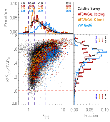
Figura 3: $X$ non-correlated variability index versus the ratio of the $K_{(fi)}^{(2)}$ correlated index to the $FAP$. The Catalina (black dots - V waveband), RR Lyrae found in the VVV survey (blue squares - $K_{s}$ waveband), and WFCAM variable stars (red and yellow crosses - ZYJHK wavebands and K-band respectively) are shown. The WFCAM results obtained in $K$ waveband are indicated by yellow circles. The lines set the cut-off values regarding those used to select NCD (blue detached line) and CD (orange detached line) variable star candidates. The percentage of data enclosed by these lines are displayed in the upper and right panels along with their respective histograms.

• The WFSC1-ZYJHK, WFSC1-K, and CVSC1 show similar distributions of $X$ values (see top panel). On the other hand, the GraMi shows a large number of sources having $X$ index bigger than $3$. This means that the WFSC1-ZYJHK, WFSC1-K, and CVSC1 samples have quite similar signal to noise distribution (Ferreira Lopes et al., 2018b) and they are more representative than the GraMi sample, i.e. those samples are more mixed, and include a larger variety of variable stars. In fact, the GraMi is a sample of RR Lyrae stars which have amplitudes that are, on average, larger than in the others samples.

• The amplitude found in optical light curves is usually larger than those found in the near-infrared light curves for the majority of variable stars (e.g. Ferreira Lopes et al., 2015a; Huang et al., 2018). Therefore, on average, the number of sources having $X$ index close to the noise limit will be bigger. Indeed, $28.4\%$ of WFSC1-K have $X<1.5$ while the proportion of CVSC1 is $16.9\%$ and WFSC1-ZYJHK is $15.7\%$ at the same cut-off. On the other hand, only $1.7\%$ of GraMi data are found in this range as expected, given the nature of the sample discussed in the previous paragraph. This indicates that a fraction of RR Lyr stars having lower amplitudes in the fields analysed by Gran et al. (2016) and Minniti et al. (2017) were missed.

• The CVSC1 and GraMi show a peak at $K_{(fi)}^{(2)}/FAP\simeq 1.55$. However, the WFSC1-ZYJHK has more stars for high or lower $K_{(fi)}^{(2)}/FAP$ values than the other distributions. It indicates that CVSC1 and GraMi missed some variable stars or it is only a sampling effect. Indeed, the CVSC1 and GraMi were not investigated using the $K_{(fi)}^{(2)}$, a new variability analysis using NITSA recommendations will resolve this question.

• About $0.1\%$ of GraMi sources do not have enough correlated measurements and so they only can be analysed using the $X$ index. Therefore the efficiency rate using $K_{(fi)}^{(2)}/FAP>1$ is nearly $100\%$. On the other hand, all of the sources in the WFSC1-ZYJHK, WFSC1-K, and CVSC1 samples are above this limit.

• The cut-off used to create the CD-CVSC implies that $\sim 99\%$ of variable stars are included in the VVV database based on the analysis of the WFSC1-K, CVSC1, WFSC1-ZYJHK, and GraMi samples. The variability indices should detect all correlated signal types, including ones not present in the already analysed catalogs, since these indices were not designed to detect any particular signal. On the other hand, the NCD-CVSC selects $\sim 71.6\%$ of the true variable sources and $\sim 27.3\%$ for $K_{s}>11.5$ and $K_{s}<11.5$, respectively. Indeed, this statistic is biased by the signal-to-noise distribution (see discussion above).

The current analysis validates the cut-offs used to create CD-CVSC and NCD-CVSC. Indeed, this diagram can be extended for past, ongoing, and forthcoming projects since the $K_{(fi)}^{(2)}/FAP$ is weakly dependent on the wavelength observed or instrumental properties. This means a real improvement on variability analysis since a single and universal parameter is enough to select complete samples.

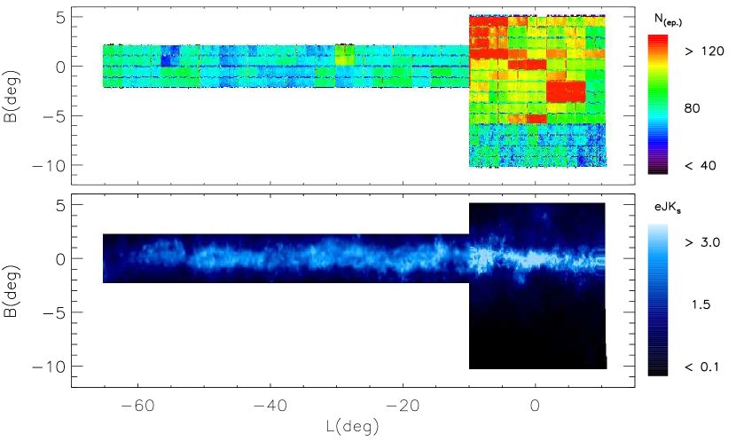
Figura 4: Spatial distribution for CD-CVSC and NCD-CVSC VVV stars with the data-points colour coded according to the number of detections (upper panel) and extinction $A_{K_{s}}$ (lower panel). The tile edges are seen in the upper panel.

4 CD-CVSC and NCD-CVSC VVV stars

Using CD-CVSC and NCD-CVSC, we have selected a sample containing $44,998,752$ sources (VVV-CVSC). About $99\%$ of variable stars detectable by the VVV survey are included in our catalogue according to our analysis (for more details see 3.4). Indeed, for each true detection there are at least $10$ MIS sources according to Ferreira Lopes & Cross (2017). A smaller number of MIS sources can be achieved using higher cut-off values available in the released tables (see Sect. A). Additionally, the $ZYJHK_{s}$ VVV photometry and the total extinction in the $K_{s}$-band ($A_{K_{s}}$) provided by the VVV extinction maps presented in Minniti et al. (2018) are available in the released tables. The mean $A_{K_{s}}$ over an area of $10\times 10$ arcmin² around the target position was used for the disc area. On the other hand, the total extinction $A_{K_{s}}$ was taken directly from the Bulge Extinction And Metallicity (BEAM) Calculator Gonzalez et al. (2012). The Cardelli et al. (1989) extinction law was assumed in both estimations.

Figure 4 shows the spatial distribution of CD-CVSC and NCD-CVSC VVV stars. The number of detections taken in the bulge is greater than in the disc. The highest number of measurements are found is b293, b294, b295, b296, b307, b308, b309, b310, as well as b333 (the tile containing the Galactic centre), where $N_{\rm ep}>120$. The specification of each tile can be found in the released table. Indeed, VVVX may improve the period detection or increase the variable candidate list as observations will be taken for all of VVV fields. There are often similar numbers of observations in groups of 4 tiles (arranged 2x2). The observing tool allows combining them in a so-called concatenation, i.e. these tiles are observed back to back together, without any other observations interloping. This is done to calculate the sky background, which in the Ks-waveband changes rather quickly. Indeed, the difference in the number of measurements within a concatenation will arise because some observations were declared failed, and deprecated: maybe the seeing degraded or there are some other concerns (like very bright stars).

Tabela 1: Variability types and counts for the crossmatched sources. The meaning of the acronyms can be found at the AAVSO and SIMBAD repositories.)

Type	Other types	Counts
ACV	ACVO, $*$alf2CVn, RotV$*$alf2CVn,	$24$
APER		$27$
BE	GCAS, Be$*$, Ae$*$, ….	$145$
BY	BY$*$,	$21$
CEP	CEP(B), Cepheid, Ce$*$, …	$64$
CV	CataclyV$*$, IBWD, V838MON, …	$54$
CW	CWA, CWB, CW-FU, CW-FO,	$814$
DCEP	DCEP(B), DCEPS, DCEP-FU, …	$393$
DSCT	DSCTC, DSCTr, dS$*$, DS	$101$
E	AR, D, DM, ECL, SD, $*$in$**$, SB$*$,	$90687$
EA	EA-BLEND, ED, EB$*$Algol, Al$*$,	$1867$
EB	ESD, EB$*$WUMa, EB$*$betLyr, …	$3167$
EW	DW, K, KE, WU$*$, KW	$24722$
EC	EC	$47498$
FKCOM	RS, RSCVn, SXARI, …	$1556$
GRB	gam, gB, SNR, SNR?, …	$27$
HADS	HADS(B), SXPHE, SXPHE(B),	$40$
HMXB	HXB, HX?, …	$13$
I	IA, IB, $*$iA,	$20$
IN	IT, INA, INB, INT, …	$33$
IR	IR$<10\mu m$, IR$>30\mu m$, OH/IR, NIR,	$2274$
ISM	PoC, CGb, bub, EmO, …	$1166$
L	LB, LC, …	$215$
LMXB	LXB,	$13$
LPV	LP$*$, LPV$*$, …	$745$
M	Mira, Mi?, Mi$*$, …	$1689$
Microlens	LensingEv, Lev	$231$
N	NA, NB, NC, NL, NR, Nova-like, …	$830$
NSIN	EllipVar, ELL,	$14564$
Others	PoC, CGb, bub, EmO, …	$72355$
PER		$261$
PUL	PULS, Pu$*$, Psr, …	$308$
Planet	PN, Pl, …	$290$
RCB	DYPer, FF, DPV, DIP, …	$18$
RGB	RGB$*$, RG$*$, …	$702$
ROT	R, RotV$*$, RotV, CTTS	$343$
RR	RR(B), RRD, RRAB, RRC, RRLyr, RR$*$	$30923$
RV	RVA, RVB, …	$143$
Radio	mm, cm, smm, FIR, Mas, …	$1084$
SR	SRA, SRB, SRC, SRD, SRS, …	$71297$
TTS	WTTS	$193$
TTau	TTau$*$, TT$*$	$31$
UG		$41$
V$*$	V$*$?,	$1299$
WR	WR$*$	$88$
X	XB, XF, XI, XJ, XND, …	$2073$
YSO	Y$*$O, Y$*$, Y$*$?	$7123$
ZAND		$26$
iC	$*$iC, $*$iN, AGB$*$, …	$6167$

Within the VVV tiles, we found a tiny region having a smaller number of detections, the blue stripes in contrast with the green and red region in the upper panel of Figure 4. This can be related with a smaller efficiency of the detector in its boundaries. On the other side, the region that links the disk and bulge VVV areas shows an increase in the number of detections (see a red line in the crossed region between bulge and disk tiles). This happens because the intersection region between the disk and bulge VVV areas has a higher number of measurements. The spatial distribution of $eJK_{s}$ values varies from $<0.1$ mag in the outer bulge up to $eJK_{s}\simeq 3$ mag for objects near the Galactic Centre. A note of caution: the total extinction as calculated by the VVV maps is certainly overestimated according to Gonzalez et al. (2018).

4.1 Cross-identification

$339,601$ VVV-CVSC sources were previously recorded by the AAVSO International Variable Star Index (VSX; Watson et al., 2014) or SIMBAD database. This subsample was named as VVV-CVSC-CROS. SIMBAD contains about $9,795,519$ objects across the sky while VSX contains $1,432,959$ sources to date. These repositories contain the widest compilations of variable stars known so far that can contain names, positions, photometric information, period, variability types, and astronomical parameters such as constellation and the passband used to measure the variability. The Tool for OPerations on Catalogs And Tables (TOPCAT - Taylor, 2005) was used to crossmatch our catalogue with the SIMBAD database. The allowed tolerance of the crossmatch was $1^{\prime\prime}$ in the sky coordinates for VVV where the nearest source was assumed as the crossmatched source.

The data found in these repositories does not contain all available information in the literature. For instance, the main table of SIMBAD has variability types but does not include the variability periods. On the other hand, the VSX table contains both information. Moreover, multiple classifications or different nomenclature can be found in these tables. The acronyms identifying the variability types were used to group the sources in different branches. We took the first classification for those objects having multiple classification. Therefore we have added two columns to our table giving information about the variability type: the notation adopted by us (column $cfl.mainVarType$) and the one that comes from literature (column $cfl.literatureVarType$). The full description of available tables is given in the Sect. A.

The main information about VVV-CVSC-CROS are released in a secondary table having the following pieces of information; VVV identifiers, literature names, variability periods, and variability types when available. The VVV identifiers can be crossmatched with the VVV-CVSC table (for more details see Sect. A) to access full VVV information about these sources. Besides, further information about them can be accessed using the literature names or coordinates in web services (for more details see Sect. A). Table 1 shows a summary of VVV-CVSC-CROS having more than 10 object per variability type. The main results from this crosscorrelated database are summarized below;

• (E) About $27\%$ of the crossmatched sources are classified as eclipsing binaries, matching the $49\%$ of stars being found in double or multiple systems. Hence a larger number of eclipsing binaries is to be expected. If we include E, EA, EB, EW, EC, NSIN, and X the final rate rises to $54\%$.

• (RR) The variability type having the second largest number of crossmatched sources are the RR Lyrae. These types of stars have quite a high amplitude and short periods (e.g. Ferreira Lopes et al., 2015a; Huang et al., 2018). These properties increase the identification rate of these sources.

• (SR) Semiregular variable stars are giants or supergiants of intermediate and late spectral type showing considerable periodicity in their light changes, accompanied or sometimes interrupted by various irregularities. Their amplitudes may be from hundredths of a magnitude to several magnitudes. On the other hand, the variability periods are quite long (the range from $20$ to $>2000$ days) compared with the RR Lyrae. Therefore a smaller detection rate for these sources are expected. Indeed, the long period variables (LPVs) and Miras (M) can be included in this class.

• (FKCOM) FK Comae Berenices-type variables are rapidly rotating giants with non-uniform surface brightnesses with a wide range of variability periods and amplitudes about several tenths of a magnitude. Their detection rate is not so different from that found for X-ray type stars.

• There are many VVV-CVSC-CROS sources which have not been assigned a variability type. The identification can be related to their localization like a star in a cluster (iC), young stellar object (YSO), or part of cloud (Poc) for example. On the other hand, they also can be classified as peculiar emitters like metric/centimetric/milimetric/sub-millimetric radio sources, far/near infrared sources, or objects having emission lines.

The VVV-CVSC-CROS is a unique catalogue which can be used to study many open stellar astrophysics questions about the IR variability of a wide range of variable stars. In fact, stellar populations or a deeper analysis about the IR variability are beyond the scope of this paper. However, the light curve shapes and some comments about these objects are explored in Sect. 5.2.

4.2 Variability periods

The variability period of VVV-CVSC were estimated using five methods; Generalized Lomb-Scargle (LSG: Lomb, 1976; Scargle, 1982; Zechmeister & Kürster, 2009), String Length Minimization (STR: Dworetsky, 1983), Phase Dispersion Minimization method (PDM: Stellingwerf, 1978; Dupuy & Hoffman, 1985), and Flux Independent and L Panchromatic Period method (PK and PL: Ferreira Lopes et al., 2018a). We combined these five different period estimations with our statistics to reduce the number of MIS sources as well as to set the reliability of signal detection. A range of frequencies between $f_{min}=2/T_{tot}$d^-1 to $f_{max}=30$d^-1 and a frequency sampling of $N_{freq.}=20\times f_{max}\times T_{tot}$ were used. This frequency sampling has higher resolution than that commonly used in surveys like OGLE, Catalina, WFCAM, Gaia, as well as previous works using VVV data. However signals like EA can still be missed using this frequency grid accordingly to Ferreira Lopes et al. (2018b). Indeed, a procedure adopting a lower resolution grid that then steps up to higher resolutions if a sufficiently good quality period is not found may improve processing time. However, how to set the criteria to define a good quality period is an open question. For all the above, the choice of frequency sampling is a compromise between efficiency rate, signal type, and processing time.

Moreover, the best period estimation is determined by the signal-to-noise ratio. We created the phase diagram using each period estimation and with Fourier harmonic the fit was obtained. The signal-to-noise ratio was calculated by dividing the peak to peak amplitude by the standard deviation of the residue. The period with the highest signal-to-noise was determined to be the best one. Two columns related with the best period (FreqSNR) ant its signal to noise (SNRfit) are available in the table.

Crossmatched sources having previous estimations of variability periods from independent groups, and usually with independent data, were used to check our results. Three considerations must be kept in mind when performing an accurate analysis of the crossmatched periods: i) typos or incorrect variability periods found in the literature; ii) the signal to noise also depends on telescope and observing strategy, whereas amplitude is mainly dependent on wavelength usually varies for different wavelengths and hence the detection of a signal can be difficult if the signal to noise in the $K_{s}$ waveband is very small; iii) the data quality, number of measurements, and arrangement of observations can hinder the signal detection. Figure 5 shows the the rate of agreement between the periods determined in this work with the literature as function of number of observations, $K_{s}$ magnitude, and the X-index. Each data point was computed using five thousand sources of the VIVA catalog. The main remarks are summarized below;

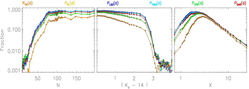
Figura 5: The rate of agreement between our period estimations in comparison with the literature period ($P_{cr.}$) as a function of the number of observations (left panel), $K_{s}$ magnitude (middle panel), and X variability index (right panel). The results considering each period estimation method are shown by different colours identified by the key at the top.

• The yield rates for $P_{LSG}$ and $P_{PDM}$ are the highest and similar to each other. $P_{PL}$ and $P_{STR}$ are slightly lower, but not too dissimilar. On the other hand, a lower yield rate is found for $P_{PK}$. The $P_{SNR}$ has a rate of agreement slightly lower than that found by $P_{LSG}$ and $P_{PDM}$.

• The $P_{cr.}$ found in the crossmatched tables are often truncated, only providing a smaller number of decimal places than those presented in this work. The large majority of these periods were from the VSX table and hence the original works of these results can have a better estimation.

• None of the parameters used as a reference leads to a yield rate of $100\%$, The highest yield rate is found when a magnitude selection is considered ($72\%$). This means that a clean sample cannot be achieved using any single parameter alone.

• The literature periods in disagreement with those computed in this work are mainly those related with semi-regular variables and eclipsing binaries. Eclipsing binaries and semi-regular variables are strongly dependent on the number of measurements and signal-to-noise ratio since these sources can have low amplitudes and the statistical significance of all variability sources depends on these parameters. In particular, eclipsing binaries having a small phase range in eclipse are easily missed with a few measurements (see bottom right panel of Fig. 6). On the other hand, the rate of agreement for the RR stars can achieve $\sim 92\%$ if the X index is take in account.

• About $39\%$ of detected periods are harmonics or aliases of $P_{cr.}$. These peculiarities must be taken into account when classifying the variables.

• Seasonal periods are more likely to be selected using the LSG, PDM, and STR methods. On the other hand, the $P_{PK}$ and $P_{PL}$ do not show strong lines related with seasonal variations but they show more sources related with higher harmonics of $P_{cr.}$. Moreover, some parallel lines that do not correspond to harmonics also appear when the periods are compared.

The rate of agreement depends of the number of observations, magnitude, variability indices, among other factors. Therefore, we visually inspected the phase diagrams folded with $P_{cr.}$ as well as those periods estimated by us in order to understand the differences. Our conclusions are based on a quick visualisation of sources having more than 30 measurements. Three main groups can be found when the estimations of variability periods are different (see Fig. 6), such as;

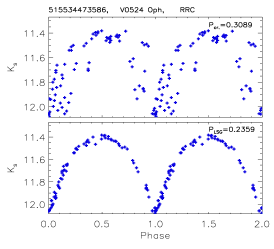
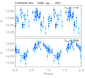
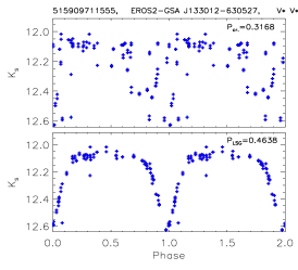
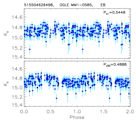
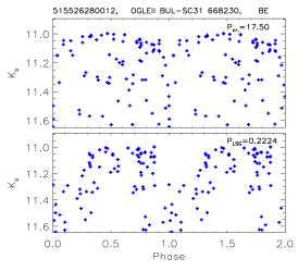
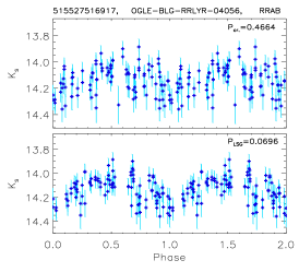
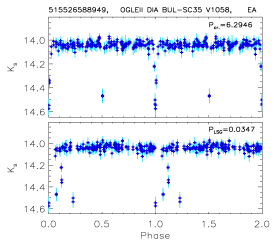
Figura 6: Phase diagrams of crossmatched sources. In each set of panels we show the phase diagrams created using $P_{cr.}$ (upper panel) and with our period (lower panel). The periods used are displayed in the upper right corner of each panel while the VVV-ID, name, and variability types are in the title.

• (Upper panels of Fig. 6) - $P_{cr.}$ is not accurately estimated or the corresponding variation is not found in the VVV-$K_{s}$ data. Indeed, sources that change their period over time can provide different results for different epochs. However, if these sources are not changing their periods, this result indicates that $P_{cr.}$ is wrong since the period estimated by us provides a smooth phase diagram. On the other hand, a second possibility although unlikely, is that the variations observed in the $K_{s}$ band may be different to those ones observed in other bands. The third possibility is that the available $P_{cr.}$ is not accurate enough to return smooth phase diagrams. In this case, both estimations may be correct or they may be harmonics of the main period.

• (Middle panels of Fig. 6) - Neither the folded phase diagram with $P_{cr.}$ nor that using our period estimate are smooth. The phase diagram folded with our periods seems smoother than those found by $P_{cr.}$ for a large number of sources. These types of objects are the vast majority of not-matching crossmatched periods. Indeed, we are using aperture photometry and hence nearby stars, diffraction spikes and other biases related with crowded regions may affect the measurements.

• (Lower panels of Fig. 6) - The period estimated by us is wrong or it is not in agreement with $P_{cr.}$. The arrangement of measurements found for the periods estimated resemble a smooth phase diagram but they are related with seasonal variations. Variations on zero point calibration also can cause such variations. Indeed, such cases correspond to a small fraction of crossmatched sources. This highlights the importance to check other information besides the folded phase diagrams to determine the true variability periods in order to return a reliable classification.

The periods estimated by us usually provide equally smooth or even smoother phase diagrams than those found for $P_{cr.}$ when these periods are in agreement (see Fig. 7). However, our periods can be related with the first harmonic of the true variability period. For instance, the top line of panels shows eclipsing binaries where the OGLE periods are twice those computed by us. The constraints used to determine if the period is double for eclipsing binaries were not considered since a detailed analysis of the symmetry of the eclipses in comparison with pulsating stars is required. Indeed, there are several types of light curves that are very difficult to distinguish: contact binaries with ellipsoidal variations (low inclination eclipsing binaries) and RRc Lyr. Therefore, more information is needed because they shared the same range of periods, amplitudes, shape, and so on. Indeed, sometimes even with visual inspection it is very difficult to determine the variability type if more information is not added. For all these reasons, the harmonics or overtones of the period computed by us were not checked. For instance, the periods of variable stars reported by the Catalina survey where checked and as a result we observe that about $50\%$ of them are double that found at the highest periodogram peak (Ferreira Lopes et al. submitted). Therefore, a similar or higher rate of matches could be expected in the current catalog since the amplitude and number of observations is smaller that that found in the Catalina data.

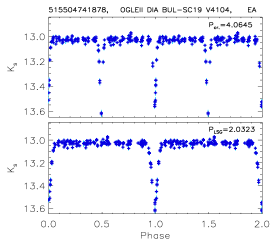
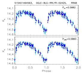
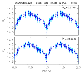
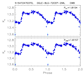
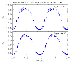
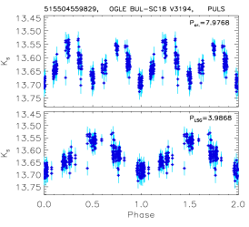
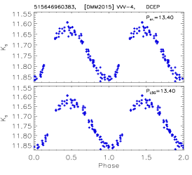
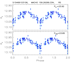
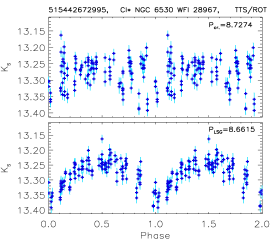
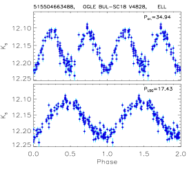
Figura 7: Typical light curves of VVV-CVSC catalog. The phase diagram using the variability periods found in the literature and those estimated in this work are displayed in the upper and lower panels of each plot, respectively.

Figura 8: Relative density plots of the ratio of PK power versus FAP as function of the variability period $P_{LSG}$ in the centre panel. The histograms corresponding to x and y axis are shown at upper and right sides. The histogram corresponding to the crossed sources having matching periods is shown in orange in the right panel. The maximum number of sources per pixel is shown at the top-right of the central panel. The aliasing periods are easily seen at the histogram peaks. On the other hand, the long timescale period cut off is set by the total time span of our observations.

In summary, the period estimation in this work provides an independent method to check previous estimates, to study the corresponding variations in multi-wavelength data, and to search for new variable stars. The crossmatched sample only corresponds to $\sim 0.5\%$ of the VVV-CVSC catalog, i.e. the $\sim 99.5\%$ sources of our sample constitutes a number of potentially new objects with variability information for the heavily crowded and reddened regions of the Galactic Plane.

4.3 Main variability periods

The main variability period estimated for the five methods are available in the release and hence the user can adopt the one that fits best for his/her purpose. For instance, the STR method is more suitable than other methods for detecting eclipsing binaries since it has the highest yield rate for these kinds of objects. On the other hand, when all variables star types are considered, LSG and PDM method provide better results (e.g. Ferreira Lopes et al., 2018b). Indeed, our results also confirm that the highest yield rates are found for LSG and PDM methods (see Sect. 4.2). In order to facilitate the forthcoming discussions, we adopt as the main variability period the one estimated by the LSG method ($P_{LSG}$). In fact, the reliability of the detected signal should be higher when all methods are in agreement.

The period power spectrum heights (PPSH - here labelled just as $H_{method}$, e.g. $H_{LSG}$), found by the five methods can vary with the number of measurements, error bars, and amplitude. In particular, the $PK$ period finding method was designed from the $K_{(fi)}$ index and hence they will have similar properties, i.e weak dependence on the instrumental properties and outliers. Therefore, $PK$ was chosen to test the reliability of the signals, which is one of our main concerns.

Figure 8 shows $PK/FAP$ ratio as a function of the main variability period $P_{LSG}$. The vertical lines found in this diagram are related to seasonal variations, i.e. $1/M$ for all $M\geq 1$ ($1d$, $0.5d$, $0.33d$, $0.25d$, $\cdots$) that are usually known as "aliasing". Moreover, weak lines are also present that can vary from one tile pointing to another. For instance, the long periods of hundreds of days, i.e. $375.35706$, $333.56015$, $345.76831$, $238.91038$, $193.00734$, $98.301643$ among others are also present in this diagram but they are more evident when the results on each VVV tile are compared individually. In order to facilitate the identification of spurious periods a flag around these lines was added. We count the number of sources having similar period values with a precision of $10^{-6}$ and $10^{-7}$ in frequency space. As a result, an integer number ranging from $1$ to more than $1000$ giving the number of periods inside in a box with a width of these intervals was set as a flag, i.e. larger numbers indicates spurious periods. These parameters are useful for quality control (for more details see Sect. 4.4). An important note, this flag is calculated in each VVV tile separately and hence the spurious periods can be slightly different from one VVV tile to another.

4.4 Getting reliable targets

According to Ferreira Lopes & Cross (2016) the sample selected using $K_{(fi)}$ returns a contamination ratio, understood as the number of total stars in our sample to the number of true variables, of about $12.6$ to select $\sim 90\%$ of the variable stars. The reader should understand contamination rate as a combination of missselection and those ones where the variability type can not be determined. Therefore, the number of variable stars where period, amplitude, and light curve shape can be studied will be a fraction of the VIVA catalog. The staset and constraints used by Ferreira Lopes & Cross (2016) are different to those adopted in this work. Moreover, we are returning a complete sample and hence we must assume there is a contamination rate of at least 10. Therefore, the available parameters should be used to restrict the sample when more reliable samples are required.

Indeed, the fit to the phase diagram can be more easily found using harmonic fits (e.g. Debosscher et al., 2007; De Medeiros et al., 2013; Ferreira Lopes et al., 2015b, c) and hence many parameters that reduce the misselection rate and are useful for classification can be obtained. Classification will be undertaken in a forthcoming paper of this series. On the other hand, a clue about the reliability of the signal is found straightforwardly from the height or power of the period found by one of the methods. Indeed, this assumption depends on the signal type for LSG method, for example, i.e. signals mimicking sinusoidal variations have a greater height in the period power-spectrum compared to other signals with the same amplitude. The power or height is greater for light-curves that return a smoother - i.e. less scatter from a simple functional fit - phase diagram when folded on that period. Non-smoothed results such as incorrect periods or aperiodic signals return the expected height for noise. However, peculiarities of each method combined with statistical fluctuations can appear in a non-smoothed phase diagram as a good detection.

The WFSC1-ZYJHK, WFSC1-K, CVSC1, and GraMi samples were used as comparison stars (for more details see Sect. 3.4). The period power spectrum heights (PPSH) were computed for those comparison stars in the same way as for the VVV-CVSC data (for more details see Sect. 4.2). However, the $K_{(fi)}$ is computed using multi-wavelength data in order to have correlated measurements, but the $H_{PK}$ is computed for each waveband separately since there is no requirement for correlated measurements. Figure 9 shows a comparison of the PPSH for the five period finding methods. For these methods, we found that:

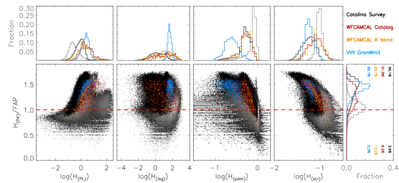
Figura 9: Power spectrum height of PL, LSG, PDM and STR methods as function of ratio of PK power height by its FAP. The grey pixels show the CD-CVSC and NCD-CVSC results while the comparison stars are presented in colours. The same colours used in the Fig. 3 are also used here for the comparison stars.

• Less than $4\%$ of comparison stars belonging to CVSC1 have $H_{PK}/FAP$ smaller than 1. However, this is a larger proportion than that found for the $K_{(fi)}/FAP$ statistic. This happens because the folded light curves seem to have a lower signal to noise than those analyzed in time, i.e. cycle by cycle.

• The same behaviour that is seen for the CVSC1 and WFSC1-ZYJHK and WFSC1-K samples, i.e. a higher fraction of sources having $H_{PK}/FAP<1$ than $K_{(fi)}/FAP<1$. The percentage of sources in the WFSC1-K group are much higher than the CVSC1 sample. The reduction in the number of measurements used to compute $H_{PK}$ together with those factors discussed in the previous item are the reasons for the lower yield rate compared with $K_{(fi)}$ index.

• Indeed, $99.6\%$ of the VVV GraMi sample are above this limit. On the other hand, the WFSC1 and its subsample in the $K_{s}$ waveband have $8.2\%$ and $13.2\%$ with $H_{PK}/FAP<1$,respectively. Not all WFSC1 sources where detected in all wavebands and hence the percentage of sources having $H_{PK}/FAP>1$ should be bigger.

• The GraMi and WFSC1-$K_{s}$ were observed in filters covering a similar wavelength range. Moreover, the yield rate of the GraMi is greater than the CVSC1 sample that is observed in the optical wavelengths. The amplitude, and hence the signal-to-noise ratio, of RR Lyrae stars are usually higher than a heterogeneous sample. Therefore, a higher yield rate found for the GraMi sample is expected.

• The $H_{PL}$ shows a clear separation between CVSC1 in comparison with WFSC1 or GraMi samples. The $H_{PL}$ depends on the signal amplitude and error bars. Therefore, this difference is related with the combination of higher amplitudes and smaller error bars since, on average, the optical wavelengths have smaller error bars and higher amplitudes than IR wavelengths.

• GraMi sample has high $H_{LSG}$ values and they are very concentrated at $H_{LSG}\simeq 80$. For example, this happens because the morphology of RR Lyrae stars is closer to a sinusoidal signal (e.g. Ferreira Lopes et al., 2015a) than for instance the one from eclipsing binaries. Indeed, a large fraction of the WFSC1 and CVSC1 samples are made up of eclipsing binaries. As expected, the results of WFSC1 and CVSC1 data are more spread because they are more heterogeneous samples.

• The CVSC1 data seem to form two connected branches in panel 3. The WFSC1 sources lie along the main branch on the right side ($\log{(H_{pdm})}>-0.5$) of the CVSC1 data while the GraMi sources lie within the left branch of $H_{PDM}$ values. The number of sources in CVSC1 is $\sim 170$ times bigger than WFSC1. Therefore, the two branches observed in CVSC1 are not so evident in WFSC1 data. Moreover, the large part of CVSC1 is composed of eclipsing binaries (usually having high amplitude and signal to noise) and hence the branches can be related to high and low signal to noise data since the first one minimizes the merit figure.

• The $H_{STR}$ increases seems to have a linear variation with $H_{PK}/FAP$ values. Moreover, the peak of the distribution found for GraMi coincides with CVSC1 despite the last one being less concentrated. The $H_{STR}$ varies with the signal-to-noise ratio and number of measurements where a larger signal-to-noise ratio and a larger number of measurements leads to a smaller $H_{STR}$ value. These aspects explain the differences found among these samples for the same reasons discussed for the other methods.

Overall, the height of the power spectrum of methods used in this work can help reduce the number of misselections. In particular, $H_{PK}/FAP>1$ includes about $\sim 97\%$ of crossmatched sources (see Fig. 9) having crossmatched periods. Moreover, it also results in a yield rate bigger than $\sim 90\%$ for CVSC1, WFSC1, and GraMi samples. These results show that $H_{PK}/FAP$ is a good indicator of the reliable signal with a single cut-off value independent of wavelength observed. Indeed, a small fraction of variable stars will be missed if only one of these methods is used. Hence, the selection criteria can be improved if different methods are combined. Moreover, the results of different methods can be combined to improve the selection criteria. For instance, the furthest left and furthest right panels of Fig. 9 have some regions that do not contain reliable signals. The height for the main period detected by each method is available in the released table where the user can select them as desired.

The flags associated with the variability period and the estimation of the amplitude can help to locate the values above which reliable signals can be found. We use the crossmatched sources having matched periods, named as VVV-CVSC*, to analyze these parameters. This consideration ensures that the signal was detected in IR light curves. We discuss how to use these flags to select targets below;

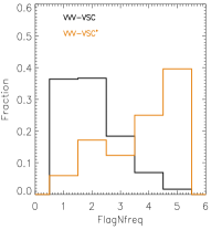
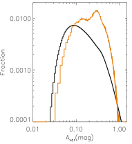
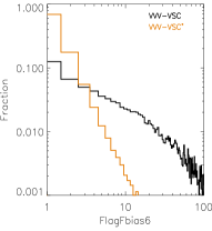
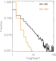
Figura 10: Histogram of FlagNfreq (upper left panel), and $\bm{A}_{VAR}$ (upper right panel), FlagFbias6 (lower left panel), and FlagFbias7 (lower right panel) for VVV-CVSC (black lines) and crossmatched sources having matched periods VVV-CVSC* (orange lines).

• FlagNfreq gives the number of periods in agreement between the five different methods (see Sect. A). We consider that the agreement is found when the period is equal within an accuracy of $10\%$ or when they are matched with the first harmonic or first overtone. The percentage of periods in agreement with the $P_{LSG}$ for VVV-CVSC is $\sim 36.6\%$, $\sim 18.4\%$, $\sim 6.9\%$, and $\sim 1.7\%$ for two, three, four, and five methods (see up left panel of Fig. 10). This means that there are at least 4 million good detections if four periods in agreement provide trustable parameters. Indeed, $\sim 73\%$ of the VVV-CVSC* (see orange lines in upper left panel of Fig. 10) meet this criterion. The FlagNfreq is the number of different methods that have a large PPSH for the best period (within 10% or the first harmonic/overtone). Periods that are matched by more methods are more likely to be correct. However, the efficiency of detection is not the same for all methods and it can vary with the signal type (see Sect. 4.3). For example, about $\sim 36.4\%$ of $P_{LSG}$ do not correspond to any other method but that does not necessarily mean that all of these periods are unreliable. Indeed, $P_{LSG}$ and $P_{PDM}$ have similar results as well as efficiency rates (Ferreira Lopes et al. submitted) and therefore the agreement between them can be used to improve the selection criteria.

• $\bm{A}_{VAR}$ denotes the amplitude of the light-curves: calculated by subtracting the $5th$ and $95th$ percentile magnitude measurements (see Sect. A). Applying the estimation of amplitude by $\bm{A}_{VAR}$ to eclipsing binaries of Algol type and similar morphologies will be biased since these sources usually have few points at the eclipse, and these few will likely be removed in the clipping. These estimations work well for a large majority of variable stars such as those undergoing stellar pulsation or some kind of semi-regular variations. Almost all VVV-CVSC* stars have a $K_{s}$ amplitude greater than $0.1$mag. Indeed, this result is a selection effect. On the other hand, only about $\sim 50\%$ of VVV-CVSC stars have amplitudes above this limit (see up right panel of Fig. 10). Indeed, the detection of variability does not necessarily mean a measured variability period, i.e. aperiodic signals or sources having enough variation to be detected by variability indices but not by period finding methods. Therefore, the use of $\bm{A}_{VAR}$ will depend of the purpose of users.

• FlagFbias6 and FlagFbias7: the detection of a signal does not necessarily mean a reliable detection since seasonal variations (or aliases) can also lead to a smooth phase diagram (see Fig. 6 last panels). These variations can be present in a large number of sources. Therefore, we count the number of periods found per VVV tile in bins of $10^{-6}$d^-1 and $10^{-7}$d^-1 (see flags FlagFbias6 and FlagFbias7). These parameters indicate the probability of the period be related to instrumental or seasonal variations since on average the number of variable stars with the same period should not be large. For instance, the probability of finding more than $10$ sources in a bin of $10^{-7}$d^-1 sorted randomly can be easily estimated. The number of sources per VVV tile is typically less than $1.5$ million sources. The probability of it having a frequency in this range will be $10^{-8}$ if we consider that a variable star can assume any value in the interval of periods ranging from zero to $1000$ days We should note, however, that true variable stars also can be flagged if they have the same period as those found to be unreliable signals.

  Figure 10 shows the histograms of FlagFbias6 and FlagFbias7 to VVV-CVSC and VVV-CVSC* stars. As expected, the VVV-CVSC* stars have flag values smaller than 10. A yield rate bigger than $\sim 95\%$ is found if a flag number smaller than 5 is adopted. On the other hand, the VVV-CVSC stars have more than $\sim 67\%$ of sources with FlagFbias6$>5$. This indicates that a large fraction of these periods can be related with seasonal or instrumental variations since large FlagFbias6 values are found for these periods. For instance, the FlagFbias6 for periods of about 1 day (i.e. $1\pm 10^{-6}$) is on average $100$ periods per VVV tile.

In summary, users can select the set of variability indices to reduce the number of stars. Moreover, the probability to detect the correct variability period will increase with the number of measurements and hence a number larger than 10 can be adopted, depending on the user. The PPSH also indicates which sources have reliable signals. Finally, the flags FlagFbias6-7 indicates the reliability of periods and if they are related with spurious variations.

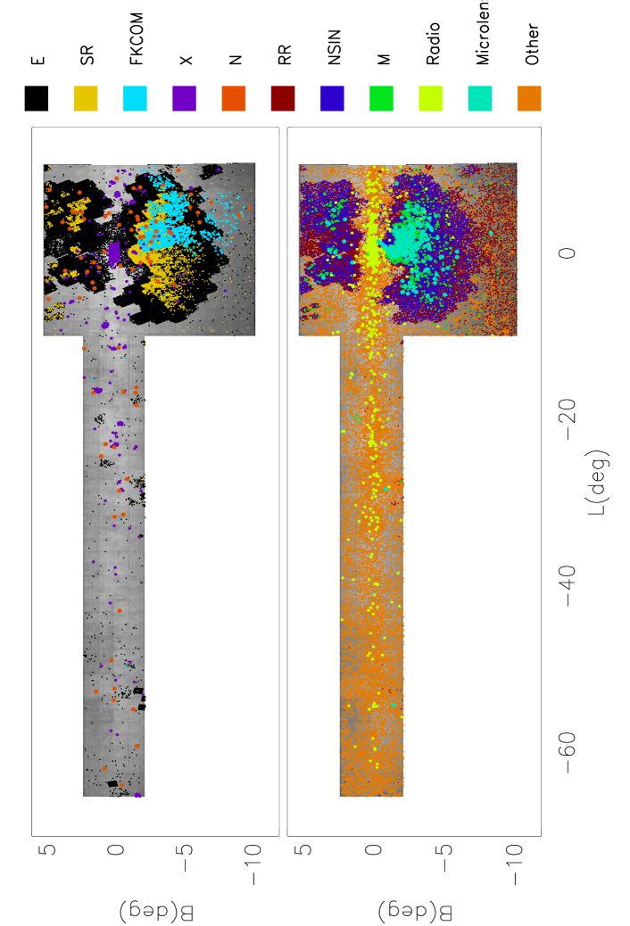
Figura 11: Spatial distribution of VVV-CVSC stars (grey colour) in Galactic coordinates for all VVV-CVSC (left panel) and for a strict selection considering the flags (right panel - for more details see Sect. 4.4). The crossmatched sources are set by colours (see the labels at the right side).

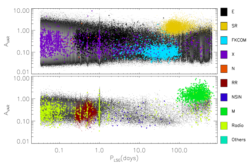
Figura 12: Amplitude ($\bm{A}_{var}$) versus variability period ($P_{LSG}$) for all VVV-CVSC (upper panel) and for a strict selection considering the flags (lower panel - for more details see Sect. 4.4). The crossmatched sources are set by colours (see label at right side).

5 Results and discussions

In this work we present an unique near-IR dataset of variable sources based on VVV photometry to investigate different matters of stellar variability. The main goal of this work is to release this variability analysis of the VVV survey. Forthcoming studies will address subjects from classification to peculiar IR variations. In the next sections, we trace an overview of the spatial distribution, colour-colour diagrams, and variability parameters in order to glimpse possibles scientific cases.

5.1 Spatial distribution

Figure 11 shows the spatial distribution of VVV-CVSC stars. The number of sources is slightly greater for the regions having more measurements. However, the same behaviour is not observed when only the crossmatched sources are considered. These distributions can be understood in terms of Galactic structure and wavelengths observed. Our main remarks are described below;

• The large majority of orange dots (other - see Sect. 4.1) means detection of unclassified sources having some IR counter-part (see lower panel). Therefore, these sources cannot be interpreted in terms of the stellar population since no information about stellar evolution is available. However, they are spread along the plane and bulge areas with a concentration about the middle regions observed by VVV. The sources having radio emission (yellow bright dots in lower panel) are concentrated in this mid-plane region.

• In terms of variability detection, a smaller number of objects is seen in the innermost bulge area and inner galactic plane. This region is usually avoided by optical surveys and amateur astronomer observations due to the high extinction that hinders the detection of variable stars. This “zone of avoidance” is also present in the distribution of the VVV Novae catalogue Saito et al. (2013) and is evident in the Gaia-DR2 LPV catalogue release (Mowlavi et al., 2018) where the innermost regions are weakly populated. Indeed, this region is not actively avoided, but Gaia has a limited number of windows that can be assigned at once, so in very crowded regions the incompleteness increases. On the other hand, the highest density of sources are found in the intermediate bulge region ($-3^{\circ}>b>3^{\circ}$) and caused mostly by eclipsing binaries (E), RR Lyrae (RR), and semi-regular (SR) variable stars detected by variability surveys mainly at optical wavelengths.

• The largest contribution of crossmatched sources comes from the Optical Gravitation Lensing Experiment (OGLE). OGLE is an optical survey which took many observations for the lower bulge region (see Fig. 1 in Wyrzykowski et al., 2015). The OGLE observations cover large sky areas where the most overlap with VVV is found in the disk and the outer bulge Milky Way areas. A study using the OGLE and VVV light curves, optical and IR wavelength, will provide clues about interstellar absorption as well as the stellar physical processes.

• The density of SR stars found in the southern bulge region ($b<-3$) is much higher than that found in the northern bulge region ($b>3$). Similar behaviour is found for Mira type stars (M). SR main sequence stars usually have small amplitude and semi-periodic variations and hence their detection requires more measurements in comparison with RR stars, for example. On the other hand, M stars need a large coverage time to be detected. The numbers of detected SR stars is growing quickly with dedicated surveys like the CoRoT and Kepler surveys (De Medeiros et al., 2013; McQuillan et al., 2013; Ferreira Lopes et al., 2015b). These results indicate that the population of SR stars is much larger than that found in Fig. 11 and the spatial difference is not real, i.e. the population studies are limited in terms of total time span and the cadence of observations.

• We expect that metal-rich RR Lyrae should be located in the Galactic disk while metal-poor RR Lyrae should be located in the bulge region (e.g. Binney & Merrifield, 1998). A large number of VSC stars in the Galactic disk give a unique opportunity to significantly increase the numbers of RR type I stars at this region since we have a limited presence of crossmatched sources in this region.

• The eclipsing binaries are mainly found in larger numbers in the Galactic bulge. The VVV-CVSC provides an opportunity to fill the empty areas of the disk since a large number of these objects are expected along all Galactic regions.

• A large number of X-ray sources were found at the Galactic centre. The variability behaviour of many of these stars has not been addressed so far. Indeed, the X-ray and XMM observations are mainly taken towards the Galactic centre and hence the large numbers of sources found in this region. The precision of X-ray coordinates are much worse than Optical or IR observations. Hence the X-ray crossmatched sources must be verified carefully. The stellar physical process related with these stars can be explored using spectroscopic follow-up together with IR light curves.

To summarize, from the spatial distribution viewpoint, the VSC catalogue offers a unique opportunity to cover regions under-explored by previous missions as well as to give new insights into those stars where the variability nature is unknown.

5.2 General variability properties

Figure 12 shows the variability periods as a function of Ks-band amplitudes found in the IR light curves. The crossmatched data having previous variability periods are labelled by colour. The upper panel shows results for the entire VVV-CVSC (grey colour) while the lower panel only shows that for those sources having (A) $X>2$, (B) $N>30$, (C) FlagNfreq$\geq 2$, (D) FlagFbias6 $\leq 2$, and (E) $H_{PK}/FAP>1.0$. Criteria (A) removes low signal-to-noise ratio data and misselected sources, (B) removes the sources where there is a low probability to estimate good periods, (C) and (D) remove the sources where the periods are not in agreement or they are probably related with a dubious period from aliasing or seasonal effects, while (E) keeps only those sources where the strength of variability period is greater than the white noise value considering a sinusoidal variation. Different astronomers can use these parameters or other combinations of criteria to select samples that suit their science. Publishing a more complete catalogue with parameters to select reliable samples save time of all users. These constraints reduce the sample to about one million sources. A large fraction of sources outside of these limits are not reliable signals (for more details see Sect. 4.4). The periods plotted for the crossmatched sources are those found in the literature when available otherwise those ones computed by us are used. Indeed, detection of variability does not mean that periodic features will be present or measurable. The main concerns about the period versus amplitude distribution can be summarized as follows:

• The VVV-CVSC sources show a lower limit of $\bm{A}_{VAR}\simeq 0.01$ magnitudes in $K_{s}$ considering the entire sample. On the other hand, the strict selection performs a lower limit of $\bm{A}_{VAR}\simeq 0.05$ magnitudes in $K_{s}$. It seems that this is the lower detection limit of the VVV survey. Indeed, we are looking at the Rayleigh Jeans tail of the stellar fluxes and hence the amplitudes are smaller than in the optically selected variable stars. Therefore, FKCOM, NSIM, and other sources having $\bm{A}_{VAR}$ smaller than this limit will be missed, for instance. Indeed, the crossmatched sources (lower panel) have $\bm{A}_{VAR}$ value distributed along the whole range of amplitudes detected by VVV observations. Moreover, for this sub-sample, the number of sources with periods equal to seasonal periods are reduced.

• The peaks in the distribution due to seasonal variations also appear in the strict selection. This happens because seasonal variations and true signals can have periods around 1 day and aliased phase diagrams (see OGLE II Dia BUL-SC12 V0700 in Fig. 6). Signals about these peaks must be considered carefully. On the other hand, "data mining" of signals having amplitudes smaller than $\bm{A}_{VAR}\simeq 0.05$ is hindered since sources with these amplitudes are dominated by a large number of noisy or unreliable signals.

• The limits on the range of periods used to discriminate different variable stars types are not well defined, as expected. On the other hand, the mean amplitude for M ($\bm{A}_{VAR}\simeq 0.96$mags) and SR ($\bm{A}_{VAR}\simeq 0.77$mags) type stars are much larger than other ones since they have long variability timescales. The FKCOM variable stars have mean variability periods of $\sim 37$ days and an amplitude of about $\sim 0.06$ mags.

• Aperiodic variable stars, long period variables (LPVs), low amplitude variables, and all other variable stars where the complete variability phases was not covered by VVV observation can have $H_{PK}/FAP<1$ and this will reduce their completeness in strictly selected samples.

• Radio and X-ray sources have no variability periods previously estimated. Many of them are related with the aliases of one day. The other ones must be checked in order to determine the IR variability counterparts to these detections.

• The variability indices indicate an intrinsic variation while the amplitude shows the signal strength at 2 microns. Indeed, the amplitude is helpful to discriminate those sources having characteristic amplitudes like Miras (M) stars.

• For periodic variable stars, the light curve shape can be easily accessed from the phase diagram folded by its variability period in order to facilitate its classification.

This catalog is a unique tool to identify variable types in terms of amplitude and variability periods from already available data. Indeed, the limits that are required to create a reliable or complete selection depend on the purpose of each user. Once this has been decided, the users can download the light curves and tables in order to combine colour information and shape parameters that can be easily computed from the light curves. Figure 7 shows some examples of data quality and a wide number of variability types that can be accessed from the VVV-CVSC. Users should realize that the variability periods found by us correspond to the first harmonic of a large minority of sources (see Sect. 4.2). Therefore, the analysis of the harmonics must be addressed before fully analysing the data.

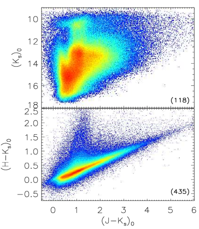
Figura 13: $(J-K)_{0}$ versus $(K)_{0}$ colour-magnitude diagram (upper panel) and $(H-K)_{0}$ vs $(J-K)_{0}$ colour-colour diagram (lower panel). The higher number of sources per pixel is shown in the right corner in each diagram. We should probably note that the brightest sources with $Ks<11$ mag are saturated.

5.3 Colour-colour and colour-magnitude diagrams

Sections 5.1 and 5.2 discuss the VVV-CVSC catalog from a framework of spatial distribution and variability parameters (amplitudes and periods). The spatial distribution of VVV-CVSC is important because it is not possible to obtain the variability parameters of the entire VVV-CVSC. Aperiodic variable stars, low signal-to-noise ratio data, saturated stars, reduced number of measurements among other things hinder this achievement, i.e. variability periods, amplitude, and morphology of variation of a large fraction of the variable stars included in the VVV-CVSC are not measurable despite the detection of reliable variability for many of these sources. On the other hand, colour-colour and colour-magnitude diagrams provide additional clues about the stellar evolution stages and hence allow us to speculate about the reasons why the variability periods are not accessible. The VVV area overlaps with many other surveys at optical and mid-IR wavelengths, see Sec.  1 which will also provide additional constraints on each star.

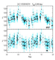
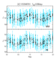
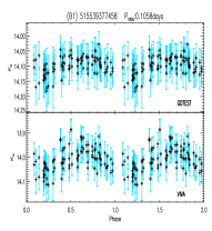
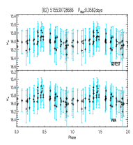
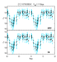
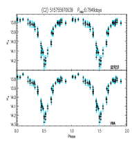
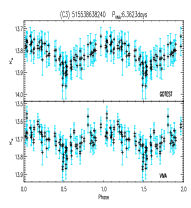
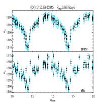
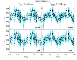
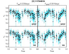
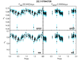
Figura 14: Phase light curves of GTEST (upper panel) and VIVA (lower panel) data. (A) and (B) panels include the sources missed in the GTEST or VIVA datasets, respectively. (C) panels shows sources having periods in agreement in both datasets while (D) panels shows variables selected in both with inconsistent periods. The phased light curves in the last line of panels are split in two columns where the first column shows the light-curve folded using the period found in the VIVA catalog (first column) and using the period in the GDTEST data (second column).

Figure 13 shows the colour-colour diagram for the VVV-CVSC dataset. The colour-colour diagram (lower panel) covers all stellar stages, i.e. the whole HR diagram. Therefore, a study of variability related to IR variations can be made using the present catalogue. On the other hand, the magnitude versus colour diagram also is quite similar to the colour-colour diagram in terms of stellar evolution. Indeed, we notice a strong reduction in the number of sources at $K_{s}\simeq 12$. This effect was also observed when the initial sample was analyzed (see Fig. 2). The cut-off value chosen (i.e. $X>1.5$) for $K_{s}<11.5$ for NC data is twice that used for fainter $K_{s}$ values. Indeed, the NCD data only corresponds to $18\%$ of the initial data. On the other hand, the CD data does not use any consideration about the magnitude and it corresponds to $82\%$ of initial data. Therefore, the gap that we are observing is related to the initial data. Users should note that, saturated objects, which may include nearby stars are probably not included in the VVV-CVSC catalogue. However, this does not explain this gap. On the other hand, the increased number of objects at $K_{s}\sim 11.0$ occurs because of an increase in the false positive rate as non-linearities and saturation effects the magnitudes despite an increased cutoff in X index (see lower left panel of Fig. 2).

Herpich et al. (submitted) have also presented a catalogue of VVV cross-match sources with the VSX-AAVSO catalogue. The authors analyse near-IR CMDs and spatial distributions for the different types of variables that enable them to discuss our current knowledge about variability in the Galaxy. The current knowledge about variability in the Galaxy is biased to the nearby and low extincted stars according the authors. The results of our cross-match is about four times larger than that found by the authors since we used other databases as well as VSX-AAVSO (see Sect. 4.1). A deep analysis on the near-IR CMDs and spatial distributions from a larger cross-match sample is beyond the current project. Indeed, the study of open questions about the empirical relationship of the stellar and variability parameters of RR Lyrae stars can be assessed already with the available data. All of these aspects can be better explored when the classification of VVV-CVSC takes place.

6 New Calibration of VVV Photometry

Recently Hajdu et al. (2019) identified two independent kinds of bias in the photometric zero-points on the VVV data: intra-array variations in the detector’s response, and the blending of local secondary standard stars. According to the authors the combination of these effects provide a space-varying bias in the absolute photometric calibration, and a time-varying error in the photometric zero-points on various time-scales. The authors also show that the first effect affects the absolute magnitude, while the latter can also affect the shape and amount of scatter in the light curve. These problems mainly affect crowded VVV regions.

We perform our own tests in three VVV tiles B306, B201, and D068 having $971093$, $294696$, and $934953$ sources, respectively. This subset of data was labelled as GDTEST. The two first VVV tiles are in the Galactic Bulge while the third one in the Galactic Disk. The comparison between B306 and B201 allows us to measure the bias related with the density of detected sources per field while the comparison between B306 and D068 investigates reddening effects. Indeed, the same algorithm and constraints were applied to the GDTEST data as the VIVA data, so that a straightforward comparison can be made.

Tabela 2: Total number of sources (N), along with the selected targets found in VIVA (N_VIVA) and GDTEST (N_GDTEST) datasets, as well as the number of matched sources between them (N_BOTH).

VVV Tile	N	NGDTEST	NVIVA	NBOTH
b306	971093	200177	501472	153869
b201	294696	7029	8326	5663
d068	934953	116200	141885	91830

From the viewpoint of selection criteria, the number of sources selected in the B306, B201, and D068 fields are 2.5, 1.2, and 1.2, larger than $N_{GDTEST}$ respectively. Table 2 shows the number of selected targets in the VIVA and GDTEST datasets of the anlayzed VVV fields. As expected the largest difference in the selected samples is found in B306. On the other hand, the number of sources found in B306 is almost the same as that found in D068 however the number of selected sources is $2.5$ times larger. Moreover, the number of selected sources found in D068 using VIVA and GBTEST differs by a factor of $1.2$. This indicates the problems related with the VVV photometric reduction are more strong related with extinction than density of stars. This indicates that B306 includes a large number of misselected sources if we consider that the number of true variable stars included in these fields is likely to be similar. However, the stellar populations are a bit different and hence a direct comparison of fraction of variables is too simplistic. Statistical fluctuations provided by the Hajdu et al. (2019) approach can either include (see (A) panel Fig. 14) or exclude (see (B) panel Fig. 14) sources with small amplitudes, those smaller than $\sim 0.03$ mag. Indeed, the large majority of sources not included in both datasets do not present a clear signal in the folded phase diagram.

The mean magnitudes found in B306, B201, and D068 GDTEST corrected data are about $0.12\%$, $0.03\%$, and $0.003\%$ brighter than the current VVV data, respectively. On the other hand, we also test the common selected sources in VIVA and GDTEST in order to check the period detection. We considered as matched periods those having a relative error smaller than 10% of the main period or its first harmonic for the LSG method. An agreement on period estimation of $50\%$, $87\%$, and $70\%$ was found for each field respectively. Indeed, more than $90\%$ of periods match directly and do not match via a harmonic or overtone. (C) panels of Fig. 14 show some examples where the period estimations are in agreement. The C4 panel shows a particularly striking example with large corrections. Very few stars have such strong modifications as those provided by Hajdu et al. (2019).

On the other hand, we also found sources where the period estimations are different or have a relative error bigger than $10\%$ (see (D) panel Fig. 14). For these sources, we can find period estimations where the periods estimated in GDTEST datasets seems better that the VIVA catalog (D1 panel), the opposite (D2 panel), and those ones where both estimations must be more carefully analysed (D3 panel). This indicates that the phase diagram by itself is not always enough to settle the best period, particularly for those sources having small amplitude. The results found for these sources in terms of variability indices and period estimation must be used carefully.

The comments above were created from a visual inspection on some thousand sources in order to provide a check of the period detection and data quality in three VVV tiles. The sources where the variability indices or period estimations are different are mainly related with sources having small dispersion values ($ED<0.03$) and a small number of observations (typically fewer than 40) where statistical fluctuations will be more important. In summary, the analysis performed in this work can be strongly affected, mainly for sources having sigma value smaller than $0.03$ mag or for those sources where the Hajdu et al. (2019) corrections are larger, e.g. where there is a higher source density and more blending, and where the extinction is higher.

7 Conclusions and Discussions

Data-mining of near-IR surveys is a good opportunity to test our capability to efficiently explore future variability datasets as well as investigating Galaxy regions that cannot be observed in the optical and have been explored less by previous surveys and other open scientific matters. This paper addresses the variability analysis of all VVV point sources having more than $10$ measurements using a novel approach proposed in the NITSA project. That project provided new variability indices to detect reliable signals, constraints to detect periodic signals as well as new period finding methods. These works give reliable constraints to select and detect signals in big-data sets.

In total, $288,378,769$ near-IR light curves were analyzed and as a result, we have produced a catalog $44,998,752$ of variable stars candidates (VVV-CVSC). The contamination ratio of VIVA catalog could be higher than 10 (for more details see 4.4). Five period finding methods were used to estimate the main variability periods. Moreover, our final catalog includes accurate individual coordinates, near-IR magnitudes ($ZYJHK_{s}$), extinctions $A(K_{s})$, variability indices, periods, near-IR amplitudes, among other parameters to access the science in VVV-CVSC, and is linked into the VSA where it can be used with the other VVV data and cross-matched catalogues, see § B. Users can discriminate among these parameters to select their targets of interest. Indeed, the variability detection does not necessarily mean period detection since sometimes there is not enough available data to do that or the source may not be periodically varying. Therefore, the current catalogue also can be used to select sources to be followed-up for current or ongoing surveys.

Hajdu et al. (2019) reported some problems related to the photometric calibration found in VVV dataset. We perform our own analysis in three VVV tiles in order to measure the weight of these corrections in our analysis. As expected the greatesT bias were found in the most crowded and highly-extincted VVV regions. In the future, PSF photometry of each pawprint epoch will be more suitable than the aperture photometry in the most crowded regions. Therefore, the VIVA catalog will be updated using PSF photometry in these regions.

VVV-CVSC was crossmatched with the SIMBAD and VSX-AAVSO catalogs, and a total of $339,601$ sources were in common. This subsample is a unique dataset to study the corresponding near-IR variability of known sources as well as to verify which sources did not have detected periods. Moreover, the near-IR amplitude used to select a certain classes of variable stars can also be determined from this sub-sample. On the other hand, the non-crossmatched sources is a matchless data that can be used to explore the heavily crowded and reddened regions of the Galactic plane, including stellar populations on the far side of the Galaxy. The present result also provides an important query source to perform variability analysis and characterize ongoing and future surveys like TESS and LSST.

¹National Institute For Space Research (INPE/MCTI), Av. dos Astronautas, 1758 – São José dos Campos – SP, 12227-010, Brazil
²SUPA (Scottish Universities Physics Alliance) Wide-Field Astronomy Unit, Institute for Astronomy, School of Physics and Astronomy, University of Edinburgh, Royal Observatory, Blackford Hill, Edinburgh EH9 3HJ, UK
³Instituto de Astrofísica, Pontificia Universidad Católica de Chile, Av. Vicuña Mackenna 4860, 7820436 Macul, Santiago, Chile
⁴Millennium Institute of Astrophysics, Santiago, Chile
⁵Departamento de Ciencias Fisicas, Facultad de Ciencias Exactas, Universidad Andres Bello, Av. Fernandez Concha 700, Las Condes, Santiago, Chile
⁶Vatican Observatory, V00120 Vatican City State, Italy ⁷Centre for Astrophysics Research, School of Physics, Astronomy and Mathematics, University of Hertfordshire, College Lane, Hatfield AL10 9AB, UK
⁸Instituto de Investigación Multidisciplinar en Ciencia y Tecnología, Universidad de La Serena, Av. R. Bitrán 1305, La Serena, Chile
⁹Departamento de Astronomía, Universidad de La Serena, Av. J. Cisternas 1200, La Serena, Chile
¹⁰Departamento de Física Te órica e Experimental, Universidade Federal do Rio Grande do Norte, Natal RN, Brazil
¹¹Centro de Astronomía (CITEVA), Universidad de Antofagasta, Av. Angamos 601, Antofagasta, Chile
¹²Computer Science Department, Pontificia Universidad Católica de Chile, Santiago, Chile
¹³Institute for Applied Computational Science, Harvard University, Cambridge, MA USA
¹⁴Departamento de Física, Universidade Federal de Santa Catarina, Trindade 88040-900, Florianópolis, SC, Brazil
¹⁵Universidade de São Paulo, IAG, Rua do Matão 1226, Cidade Universitária, São Paulo 05508-900, Brazil
¹⁶Núcleo de Astroquímica y Astrofísica, Instituto de Ciencias Químicas Aplicadas, Facultad de Ingeniería, Universidad Autónoma de Chile, Av. Pedro de Valdivia 425, 7500912 Santiago, Chile
¹⁷Departamento de Física, Facultad de Ciencias Básicas, Universidad Metropolitana de la Educación,Av. José Pedro Alessandri 774,7760197 Nuñoa, Santiago, Chile

Apêndice A Column description

All variability information found in this work is being released in order to facilitate forthcoming studies using the VVV database. Indeed, parameters like identifiers, coordinates, and $ZYJHK_{s}$ default magnitudes were obtained from the VISTA Science Archive while the other ones were computed in the present work. The acronyms cflvsc were added in the column description in order to identify the parameters that come from this work. Indeed, the vivaID is unique and is equivalent to the sourceID in VSA VVVDR4 data-release and hence it can be used to merge the current information with that provided in VSA tables. We have created two new tables in the VSA VVVDR4 release: vvvVivaCatalogue and vvvVivaXMatchCatalogue for the VIVA variable-star candidates (VVV-CVSC) and their cross-matched counterparts (VVV-CVSC-CROS) respectively. The two tables can be linked via the vivaID. These tables can also be found in VVVDR5 and later releases, but in these cases vivaID will not equal sourceID so a joining neighbour table will be used. Examples of how to use the VIVA data with the rest of the VVV and external data are given in the VVV Guide. The released parameters and their data types are listed below for the VVV-CVSC (vvvVivaCatalogue);

• vivaID: UID in the VIVA catalogue, equivalent to the merged band-pass detection (sourceID) in the VSA vvvSource (VVVDR4) table as assigned by merge algorithm (type: bigint, 8 bytes);

• raJ2000: celestial right ascension in degrees, from VVVDR4 vvvSource (type: float, 8 bytes);

• decJ2000: celestial declination in degrees, from VVVDR4 vvvSource (type: float, 8 bytes);

• glJ2000: Galactic longitude in degrees, from VVVDR4 vvvSource (type: float, 8 bytes);

• gbJ2000: Galactic latitude in degrees, from VVVDR4 vvvSource (type: float, 8 bytes);

• WAperMag3: $W=[Z,Y,J,H,K_{s}]$ magnitudes using aperture corrected mag (2.0 arcsec aperture diameter, from VVVDR4 vvvVariability - type: float, 4 bytes);

• WAperMag3Err: error in default point source $mag=[Z,Y,J,H,K_{s}]$ mag, from VVVDR4 vvvVariability (2.0 arcsec aperture diameter - type: float, 4 bytes)

• KsAperMagPawprint3: $K_{s}$ mean magnitude using pawprint data (2.0 arcsec aperture diameter - type: float, 4 bytes);

• ED: even dispersion parameter of $K_{s}$ pawprint data (type: float, 8 bytes);

• $ExpRMS_{N}oise$: expected noise value for even dispersion parameter of $K_{s}$ pawprint data (type: float, 8 bytes);

• NgoodMeasurements: number of good measurements found in the pawprint data (type: integer, 2 bytes);

• Xindex: X variability index (type: float, 8 bytes);

• Kfi2: even dispersion parameter of $K_{s}$ pawprint data (type: float, 8 bytes);

• L2: expected noise value for even dispersion parameter of $K_{s}$ pawprint data (type: float, 8 bytes);

• Ncorrelation2: number of correlated measurements (type: integer, 2 bytes);

• FAPcorrelation2: false alarm probability to $K_{(fi)}$ variability index (type: float, 8 bytes);

• FlagDataType: flag about data type, i.e correlated data (CCD) or non-correlated data (NCD) (type: string, 3 bytes);

• EJKs: extinction computed from Gonzalez et al. (2012) (Galactic bulge) and Minniti et al. (2018) (Galactic disk) (type: float, 4 bytes);

• EJKsErr: rms related with the three nearest EJKs estimations (Galactic disk) (type: float, 4 bytes);

• FreqPKfi2: main variability frequency using flux independent period method (type: float, 8 bytes);

• $H_{Kfi2}$: PPSH of FreqPKfi2 considering PK method (type: float, 8 bytes);

• FreqPLfi2: main variability frequency using panchromatic period method (type: float, 8 bytes);

• $H_{PL2}$: height of FreqPLfi2 considering PL method (type: float, 8 bytes);

• FreqLSG: main variability frequency using Lomb-Scargle generalized method (type: float, 8 bytes);

• $H_{LSG}$: PPSH of FreqLSG considering LSG method (type: float, 8 bytes);

• FreqPDM: main variability frequency using Phase Dispersion Minimization method (type: float, 8 bytes);

• $H_{PDM}$: PPSH of FreqPDM considering PDM method (type: float, 8 bytes);

• FreqSTR: main variability frequency using String Length Method method (type: float, 8 bytes);

• $H_{STR}$: PPSH of FreqSTR considering STR method (type: float, 8 bytes);

• BestPeriod: the best period estimation, among the five methods, based in the signal to noise value (type: float, 8 bytes);

• SNRfit: signal to noise value related with the best frequency estimation (type: float, 8 bytes);

• Avar: the difference between 5th and 95th percentile of magnitude in order to provide a rough estimation of variability amplitude (type: float, 8 bytes);

• FlagNfreq: number of frequencies in agreement with FreqLSG or its harmonic or subharmonic. It assumes values from 1 to 5 (type: integer, 2 bytes);

• FlagFbias6: counts of periods within $10^{-6}$ periods (for more details see Sect. 4.3) related with FreqLSG (type: integer, 2 bytes);

• FlagFbias7: counts of periods within $10^{-7}$ periods (for more details see Sect. 4.3) related with FreqLSG (type: integer, 2 bytes);

All this information can be used to perform a comprehensive variability search of any type of variable star. In particular, the variability frequencies and amplitudes help the users to select particular types of variable star. Indeed, the crossmatched sources can be used to set the limits on all parameters available. The crossmatched sample (see Sect. 4.1) is included in the VVV-CVSC table. However, a new table is performed in order to facilitate the identification of crossmatched sample. All parameters found in the VVV-CVSC table plus the following information are available;

• vivaID: UID in the VIVA catalogue, equivalent to the merged band-pass detection (sourceID) in the VSA vvvSource (VVVDR4) table as assigned by merge algorithm (type: bigint, 8 bytes);

• LiteratureID: the identifier found in the literature or "NONE"when the name is not available (type: string);

• CrossPeriod: variability period found in the literature or $-99999999$ when the period is not available (type: float, 8 bytes);

• MainVarType: the single variability type adopted by us to group the crossmatched sources (type: string, length: irregular);

• LiteratureVarType: the variability types found in the literature (type: string, length: irregular);

Indeed, the column MainVarType was introduced to summarize the variability types since some objects have multiple identifications according to AAVSO and SIMBAD designations and number of cross-matched sources as following:

• E: AR, D, DM, ECL, SD, SB$*$

• EA: EA-BLEND, ED, EB$*$Algol, Al$*$

• EB: ESD, EB$*$WUMa, EB$*$betLyr, EB$*$, EB$*$Planet, bL$*$, Candidate_EB$*$

• EW: EC, DW, K, KE, WU$*$, KW

• I: IA, IB, $*$iA

• IN: IT, INA, INB, IN(YY), INAT, INBT, INT, INT(YY)

• INS: INSB(YY), INST(YY), INSA, INSB, INST, Rapid_Irreg_V$*$

• IS: ISA, ISB, UXOR, Irregular_V$*$

• FU: FUOR, FUOr

• BE: GCAS, Be$*$, Ae$*$, Candidate_Ae$*$, Ae?

• UV: UVN, UVN(YY), Flare$*$

• RCB: DYPer, Erupt$*$RCrB, FF, DPV, DIP, Eruptive$*$

• WR: WR$*$, Candidate_WR$*$

• AHB: AHB0, AHB1

• BCEP: BCEPS, PulsV$*$bCep

• CEP: CEP(B), Cepheid, Ce$*$, Candidate_Cepheid

• CW: CWA, CWB, CW-FU, CW-FO

• DCEP: DCEP(B), DCEPS(B), DCEPS, DCEP-FU, DCEP-FO, PulsV$*$delSct, deltaCep

• DSCT: DSCTC, DSCTr, dS$*$, DS

• RR: RR(B), RRD, RRAB, RRC, RRLyr, RR$*$

• SR: SRA, SRB, SRC, SRD, SRS, semi-regV$*$, sr$*$

• PVTEL: PVTELI, PVTELII, PVTELIII

• ZZ: ZZA, ZZB, ZZLep, ZZO

• HADS: HADS(B), SXPHE, SXPHE(B)

• L: LB, LC, L:

• RV: RVA, RVB, PulsV$*$RVTau

• GDOR: gammaDor

• LPV: LP$*$, LP?, LPV$*$, Candidate_LP$*$

• M: Mira, Mi?, Mi$*$, Candidate_Mi$*$

• roAm: roAp

• DWLYN: V1093HER, V1093Her, V361HYA

• PUL: PULS, PulsV$*$, Pu$*$, Psr, Pulsar

• TTau: TTau$*$, TT$*$, Candidate_TTau$*$

• WVir: PulsV$*$WVir, WV$*$

• ACV: ACVO, $*$alf2CVn, RotV$*$alf2CVn

• ROT: R, RotV$*$, RotV, CTTS

• BY: BY$*$

• FKCOM: RS, RSCVnRedSG$*$, RSCVn, SXARI

• NSIN: EllipVar, ELL

• N: NA, NB, NC, NL, NR, Nova, Nova-like, Symbiotic$*$, Sy1, No$*$, Candidate_Nova

• SN: SNI, SNIa, SNIa-pec, SNIb, SNIb-pec, SNIc, SNIc-pec, SNIa-BL, SNIb-BL, SNIc-BL, SNIb|c, SNIax, SNIIn-pec, SNII, SNIIn, SNII-P, SNIIb, SNII-pec, SNII-L, SNIIP

• CV: CataclyV$*$, IBWD, V838MON, CBSS, Candidate_CV$*$, C$*$, Candidate_C$*$

• X: XB, XB$*$, XF, XI, XJ, XND, XNG, XP, XBPR, XR, XBP, XB?, Candidate_XB$*$

• HMXB:Candidate_HMXB, HXB, HX?

• LMXB:LXB

• XPR:XPRM

• AGN: AGN_Candidate

• GRB: gamma, gammaBurst, gam, gB, SNR, SNR?

• IR: IR<10um, IR>30um, OH/IR, NIR

• Radio: Radio(cm), Radio(mm), Radio(sub-mm), radioBurst, mm, cm, smm, Maser, rB, FIR, RB?, Rad, Mas

• YSO: Y$*$O, Candidate_YSO, Y$*$, Y$*$?

• V$*$: V$*$?

• RGB: RGB$*$, Candidate_RGB$*$, RG$*$

• Planet: PN?, PN, Planet?, Pl, Pl?, Minorplanet

• Microlens: LensingEv, Lev

• iC: $*$iC, $*$iN, $*$inAssoc, $*$inCl, AGB$*$, Candidate_AGB$*$, Candidate_post-AGB$*$, post-AGB$*$

• ISM: PartofCloud, PoC, ComGlob, CGb, Bubble, bub, EmObj, EmO, Em$*$, EmG, Cloud, Cld, GalNeb, GNe, Cl$*$, Cl$*$?, BrNeb, BNe, DkNeb, DNe, RfNeb, RNe, MolCld, MoC, glb, OpCl, denseCore, cor, SFregion, SFR, HVCld, HVC, HII, $*$inNeb, sh, HI, Circumstellar, cir, outflow?, of?, Outflow, out, HH

• Others: $*$, $**$, Assoc$*$, BLLac, BLLac_Candidate, Blazar, BlueSG$*$, Candidate_BSG$*$, Candidate_Hsd, Candidate_brownD$*$, Candidate_pMS$*$, DwarfNova, EP, Galaxy, GinGroup, GlCl, GlCl?, GroupG, HB$*$, HotSubdwarf, MISC, NON-CV, OH, Orion_V$*$, PM$*$, Pec$*$, QSO, RedSG$*$, Region, S, S$*$, SIN, Seyfert_1, Star, Transient, Unknown, VAR, WD$*$, brownD$*$, multiple_object

Indeed, different surveys can assume different notation but the same meaning. For instance, RR is common used as RRAB or RRLyr. On the other side, many sources have a few objects or have a single notation and hence their notations were maintained: cPNB$[$e$]$, EXOR, SDOR, FSCMa, TTS, BYDra, ACEP, ACYG, BLAP, BXCIR, SPB, PPN, PSR, HB, UG, UGSS, UGSU, UGZ, UGWZ, UGER, ZAND, DQ, AM, XM, APER, PER, CST.

Apêndice B SQL Queries

We have done all the selection from the VVVDR4 release via the VISTA Science Archive. The followinq query is designed to select light-curves using pawprint detections for sources in the range 515396075613 to 515396077613. Below we will step the curious reader through the design of this selection. The SQL Cookbook in the VSA and the VVV Guide are helpful to build up complex queries.

    SELECT v.sourceID, v.frameSetID, v.ksMeanMag,
    v.ksMagRms, v.variableClass, b.multiframeID,
    b.seqNum, b.flag, m.filterID, m.mjdObs, o1SeqNum,
    o2SeqNum, o3SeqNum, o4SeqNum, o5SeqNum, o6SeqNum,
    do1.aperMag3 as o1AperMag3, do1.aperMag3Err as
    o1AperMag3Err, do1.ppErrBits as o1ppErrBits,
    do2.aperMag3 as o2AperMag3, do2.aperMag3Err as
    o2AperMag3Err, do2.ppErrBits as o2ppErrBits,
    do3.aperMag3 as o3AperMag3, do3.aperMag3Err as
    o3AperMag3Err, do3.ppErrBits as o3ppErrBits,
    do4.aperMag3 as o4AperMag3, do4.aperMag3Err as
    o4AperMag3Err, do4.ppErrBits as o4ppErrBits,
    do5.aperMag3 as o5AperMag3, do5.aperMag3Err as
    o5AperMag3Err, do5.ppErrBits as o5ppErrBits,
    do6.aperMag3 as o6AperMag3, do6.aperMag3Err as
    o6AperMag3Err, do6.ppErrBits as o6ppErrBits
    FROM vvvVariability as v,
    vvvSourceXDetectionBestMatch AS b, vvvTileSet AS t,
    vvvTilePawPrints AS p, Multiframe as m,
    (SELECT d.multiframeID,d.extNum,d.seqNum,
    d.aperMag3,d.aperMag3Err,d.ppErrBits FROM
    vvvDetection as d,Multiframe as m where
    m.multiframeID=d.multiframeID and m.offSetID=1)
    AS do1,
    (SELECT d.multiframeID,d.extNum,d.seqNum,
    d.aperMag3,d.aperMag3Err,d.ppErrBits FROM
    vvvDetection as d,Multiframe as m where
    m.multiframeID=d.multiframeID and m.offSetID=2)
    AS do2,
    (SELECT d.multiframeID,d.extNum,d.seqNum,
    d.aperMag3,d.aperMag3Err, d.ppErrBits FROM
    vvvDetection as d,Multiframe as m where
    m.multiframeID=d.multiframeID and m.offSetID=3)
    AS do3,
    (SELECT d.multiframeID,d.extNum,d.seqNum,
    d.aperMag3,d.aperMag3Err,d.ppErrBits FROM
    vvvDetection as d,Multiframe as m where
    m.multiframeID=d.multiframeID and m.offSetID=4)
    AS do4,
    (SELECT d.multiframeID,d.extNum,d.seqNum,
    d.aperMag3,d.aperMag3Err,d.ppErrBits FROM
    vvvDetection as d,Multiframe as m where
    m.multiframeID=d.multiframeID and m.offSetID=5)
    AS do5,
    (SELECT d.multiframeID,d.extNum,d.seqNum,
    d.aperMag3,d.aperMag3Err,d.ppErrBits FROM
    vvvDetection as d,Multiframe as m where
    m.multiframeID=d.multiframeID and m.offSetID=6)
    AS do6
    WHERE v.sourceID=b.sourceID AND
    (v.ksnGoodObs+v.ksnFlaggedObs) > 10 AND
    v.sourceID BETWEEN 515396075613 AND 515396077613
    AND v.frameSetID BETWEEN 515396075521 AND
    515396075522 AND b.multiframeID=t.tlmfID AND
    b.extNum=p.tlExtNum AND b.seqNum=p.tlSeqNum AND
    t.tileSetID=p.tileSetID AND
    (p.tlSeqNum>0 OR p.tileSetSeqNum<0) AND
    m.multiframeID=t.tlmfID and m.filterID=5 AND
    do1.multiframeID=t.o1mfID and
    do1.extNum=p.o1ExtNum and do1.seqNum=p.o1SeqNum
    and do2.multiframeID=t.o2mfID and
    do2.extNum=p.o2ExtNum and do2.seqNum=p.o2SeqNum
    and do3.multiframeID=t.o3mfID and
    do3.extNum=p.o3ExtNum and do3.seqNum=p.o3SeqNum
    and do4.multiframeID=t.o4mfID and
    do4.extNum=p.o4ExtNum and do4.seqNum=p.o4SeqNum
    and do5.multiframeID=t.o5mfID and
    do5.extNum=p.o5ExtNum and do5.seqNum=p.o5SeqNum
    and do6.multiframeID=t.o6mfID and
    do6.extNum=p.o6ExtNum and do6.seqNum=p.o6SeqNum

This query can be broken into several parts:

• Selection of sources with correct attributes from vvvVariability table

• Linking each source to an epoch via vvvSourceXDetectionBestMatch table

• Getting the individual pawprint detection photometry and flags for each epoch.

The main selection is on the vvvVariability catalogue where we select sources with at least 10 good or flagged $K_{s}$ band epochs (tile epochs) and sourceID and framesetID ranges.

    (v.ksnGoodObs+v.ksnFlaggedObs) > 10 AND
    v.sourceID BETWEEN 515396075613 AND 515396077613
    AND v.frameSetID BETWEEN 515396075521 AND
    515396075522

Joining to the vvvSourceXDetectionBestMatch and joining by sourceID links to all tiles that contain the source v.sourceID=b.sourceID. The vvvSourceXDetectionBestMatch is in turn joined to vvvTilePawprints (and its companion table vvvTileSet) via b.multiframeID=t.tlmfID AND b.extNum=p.tlExtNum AND b.seqNum=p.tlSeqNum AND t.tileSetID=p.tileSetID. We also link to the Multiframe to select $K_{s}$ only epochs m.multiframeID=t.tlmfID and m.filterID=5 vvvTilePawprints tells you which pawprint detections are linked to which tile detections, but does not include the photometric measurements, so joins to vvvDetection is necessary. Infact, we require 6 joins to vvvDetection, one for each pawprint offset. However, vvvDetection is an extremely large table, 50 billion rows, with more than 100 attributes, so we do subqueries to select just pawprint data for the specific offset and with the minimal number of attributes:

    (SELECT d.multiframeID,d.extNum,d.seqNum,
    d.aperMag3,d.aperMag3Err,d.ppErrBits FROM
    vvvDetection as d,Multiframe as m where
    m.multiframeID=d.multiframeID and m.offSetID=6)
    AS do6

This selection returns a thin table of aperture photometry flags and the detection table primary key for all measurements that have an offsetID equal to 6 as table do6, which is linked to a particular epoch through the vvvTilePawprints, via do6.multiframeID=t.o6mfID and do6.extNum=p.o6ExtNum and do6.seqNum=p.o6SeqNum.

Apêndice C Acronyms list

The current section was introduced in order to facilitate the identification of the acronyms found along the paper. A wider definition, of the main acronyms used along the paper, are presented below;

• A3: default aperture of 1 arcsec. This has a radius of 3 pixels and contains $\sim 75\%$ of the total flux in stellar images;

• CD: CD means data where correlated indices can be used properly. On the other hand CD-CVSC are the variable stars candidates that where selected using correlated indices;

• $K_{(fi)}^{(s)}$: it means the flux independent indices that was used to select the variable stars in the CD data.

• FAP: The false alarm probability for $K_{(fi)}^{(s)}$ to be performed by white noise. The ratio of $K_{(fi)}^{(s)}$ by the $FAP$ sets the noise data about 1 like X index.

• GraMi: the catalogue of RRLyr stars found by Gran et al. (2015) and Minniti et al. (2017) selected from the VVV Survey. The GraMi and WFSC1 are used as comparison stars in some plots of this paper.

• $H_{method}$: means the period power spectrum heights (PPSH) that was summarise as $H_{method}$;

• NITSA: means the New Insight into Time Series Analysis project where one can found new tools and remarks about how analysis photometric data-sets.

• NCD: the NCD means data where only statistical parameters (non-correlated indices) can be used. The correlated indice applied in NCD data can be over- or under- estimated. The NCD-CVSC are the variable stars candidates that where selected using statistical parameters;

• X: means the ratio of a statistical parameter ($\sigma$) by its expected noise value ($\eta$). Such consideration imply that the noise data will be about 1;

• WFSC1: it means the WFCAM variable star catalogue where comparison stars were used to test our approach. Indeed, the acronyms WFSC1- plus ZYZHKs also means the results considering a single waveband.

• VVVDR4: it means the fourth data release of VVV data.